Abstract
This paper presents a fractional linear reservoir model as the elementary response function of hydrologic systems corresponding to the classical linear reservoir model and tests its applicability to rainfall–runoff modeling. To this end, we formulate a fractional linear reservoir model in terms of fractional calculus following the same procedure as the classical linear reservoir model and, at the simplest level, compare its performance of rainfall–runoff modeling with the linear and nonlinear reservoir models. The impulse response function of a fractional linear reservoir model, a probability density function (PDF) following the Mittag–Leffler distribution, shows nonlinearity due to its time-variant behavior compared to that of a linear reservoir model. In traditional linear hydrologic system theory, the lag and route version of a fractional linear reservoir model produces the fast-rising and slow-recession of runoff hydrographs, implying the mixed response of linear and nonlinear reservoir models to rainfall. So, a fractional linear reservoir model could be considered a fundamental tool to effectively reflect the nonlinearity of rainfall–runoff phenomena within the framework of the linear hydrologic system theory. In this respect, the fractional order of the storage relationship specifying a fractional linear reservoir model can be viewed as a kind of parameter to quantify the heterogeneity of runoff generation within a river basin.
1. Introduction
The nonlinear properties of rainfall–runoff phenomena are one of the intrinsic attributes of natural systems [1]. It is well known that analytical exact solutions might be hard to obtain from mathematical models to describe water particles’ movement within a river basin via classical calculus due to their inherent nonlinearity. To cope with this, several alternatives have been developed in hydrology; for instance, a linearization of the rainfall–runoff problems through the concept of unit hydrographs [2] or a linear reservoir model [3], as well as a numerical approach to such nonlinear models as the storage function method [4]. However, it could be difficult to figure out the fundamental explanations of rainfall–runoff phenomena only through these circumvent ways due to their own nonlinearity, as mentioned before. Furthermore, since the drainage structure of river basins could be addressed in non-integer spatial dimensions through the fractal property of channel networks [5,6,7], it is unlikely that conducting a systematic approach to rainfall–runoff phenomena will be easy within the framework of classical calculus.
Fractional calculus is a branch of mathematics that deals with the integration and differentiation of the non-integer order, which has recently been widely used in various science and engineering fields [8,9,10,11]. There can also be found recent research on fractional calculus relevant to hydrology, such as [12,13,14,15,16,17,18]. Among those, Borthwick [19] suggests the fractional order derivative of storage relationships with respect to time and, thereby, the potential to extend rainfall–runoff models rooted in linear hydrologic system theory [20,21,22,23]. However, he mainly concentrates on the fractional reformulation of the existing rainfall–runoff models based on classical calculus without inspecting its hydrologic implications. This motivates us to test the hydrologic applicability of fractional calculus to rainfall–runoff modeling. In fact, fractional calculus could be expected to provide a new approach to the existing various mathematical models that have been developed based on classical calculus; therefore, it could be a valuable tool in terms of bridging the theoretical gaps and relaxing the practical restrictions relating to rainfall–runoff modeling.
In this study, we propose a fractional linear reservoir model as the elementary response function of hydrologic systems in correspondence to the classical linear reservoir model. We formulate the response functions of a fractional linear reservoir model in terms of fractional calculus following the same procedure as a linear reservoir model. Then, a comparison was performed with the models based on linear and nonlinear reservoirs in order to test the applicability of a fractional linear reservoir model to rainfall–runoff modeling at the simplest level. It should be noted that the main purpose of this study is not to provide a new rainfall–runoff model in the complete form but to provide an elementary hydrologic response function for river basins, a fractional linear reservoir concept. As commonly observed in many classical rainfall–runoff models, such as [20,21,22,23], the concept of a linear reservoir model has been frequently used as a basic element that consists of more complicated rainfall–runoff models. Therefore, this study tries to suggest a fractional linear reservoir model as an alternative to the classical linear reservoir model, especially focusing on the distinct behavior of the former compared to the one of the latter, in order to provide a new essential tool for the reasonable and systematic construction of rainfall–runoff models.
2. Theoretical Background
2.1. Linear Reservoir Model
A linear reservoir model [3] consists of a continuity equation and a storage relationship.
where , , and represent the inflow, outflow, and storage of a linear reservoir, while is a proportional constant in the temporal dimension that specifies a linear relationship between and . Assuming to be Dirac’s delta function , amounts to an impulse response function of a linear reservoir model. Thereby, substituting Equation (2) into Equation (1) results in a nonhomogeneous linear ordinary differential equation of the first-order for with respect to time
Taking Laplace transforms of Equation (3) yields
where is the counterpart of in the Laplace transform domain. Considering a linear reservoir in the empty state at the initial (, ) and, then, omitting the second term on the right-hand side of Equation (4), can be inversely transformed into
Equation (5) is the elementary response function of the linear hydrologic system to rainfall, the so-called instantaneous unit hydrograph (IUH) of a linear reservoir model, along with a linear channel model.
2.2. Fractional Calculus
Fractional calculus has been built on the formula of Cauchy’s repeated integral for an arbitrary function [24]
where denotes an integration operator, with being the gamma function. Equation (6) indicates the n-fold integration of on . However, it is noted that the first equality in Equation (6) implies in integer numbers to the second equality in Equation (6), which holds for in real numbers with the help of . Therefore, the th-order fractional derivative of can be defined as follows.
where is a differentiation operator with being real numbers. It can be seen that the subscripts in front and back of in Equation (6) and in Equation (7) specify the interval of time of interest according to the standard notation of fractional calculus. Fractional integration is based on the mathematical structure shown in Equation (6), whereas fractional differentiation undergoes various development stages originating from the classical definition of Riemann–Liouville [25,26,27]. Equation (7) is taken from Caputo’s definition of fractional derivatives, which has recently been widely used in diverse fields owing to the better availability of the observable initial conditions in the real world than the others. Ref. [28] points out that fractional derivatives can provide the description of memory and hereditary properties of various materials and processes as recognized in the integral on the right-hand side of Equation (7), and this is the main advantage of fractional derivatives in comparison with classical integer-order models. Therefore, we focus on the applicability of fractional calculus to rainfall–runoff modeling with Equation (7); therefore, this allows for considering the global variation of hydrologic variables over time, whereas the traditional approach in terms of classical calculus only the local variation of hydrologic variables with respect to time.
2.3. Mittag–Leffler Function
The exponential function in Equation (5) can be expressed as the sum of the infinite series:
The Mittag–Leffler function is a generalization of Equation (8) [29,30]
where and are two parameters of , which could be real or complex numbers. Letting , Equation (9) reduces to Equation (8) ().
The Laplace transform relevant to Equation (9) can be defined as follows [28,29,30]
where denotes a Laplace transform operator.
3. Fractional Linear Reservoir Model
3.1. Impulse Response Function
Following [19], let the first-order derivative of with respect to time in Equation (1) be rewritten in terms of the th-order fractional derivative of
where the lower limit of fractional derivatives ( in Equation (7)) goes to 0 for convenience, which is denoted according to the standard notation of fractional calculus similar to Equation (7). It can be noticed that is raised by the power of in order to preserve dimensionality. Thereby, corresponding to Equation (3), we can have a fractional nonhomogeneous linear ordinary differential equation of the th-order for with respect to time
Similar to Equation (4), Equation (12) can be rearranged for in the Laplace transform domain
where is integer numbers dependent on . Taking inverse transforms of Equation (13) with the zero initial conditions (, ), we can get the solution to Equation (12) with the help of Equation (10)
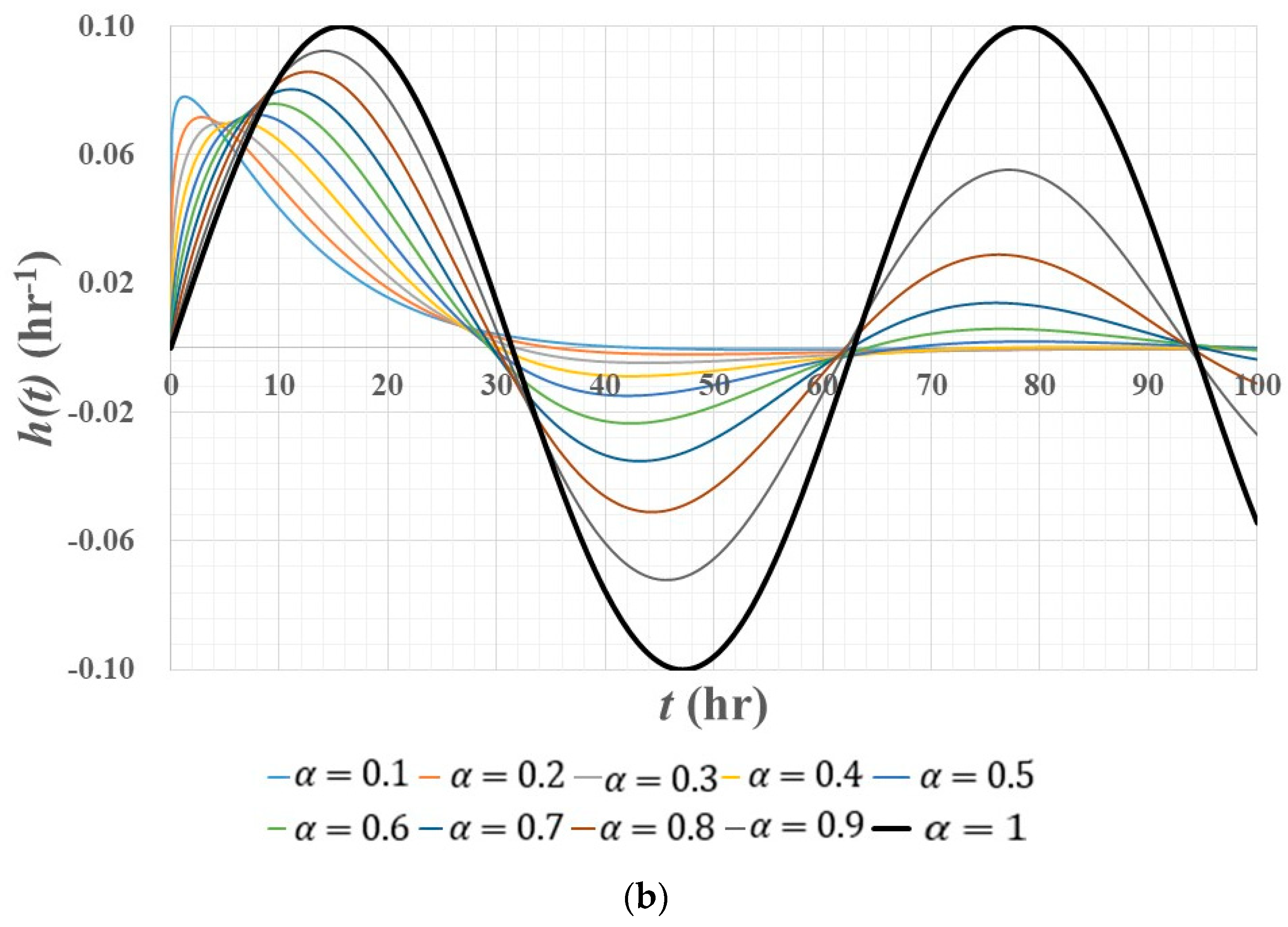
From the viewpoint of linear hydrologic system theory [31,32], Equation (14) could be viewed as the IUH of a fractional linear reservoir model. In addition, when , Equation (14) reduces to Equation (5); therefore, Equation (14) could be a generalized expression for the impulse response function of a linear reservoir model within the framework of fractional calculus. Figure 1 demonstrates in Equation (14) with , where Figure 1a depicts for while Figure 1b for . We calculate the ordinates of with the help of the Matlab code written by [33] in order to estimate .
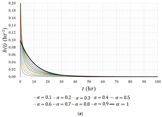
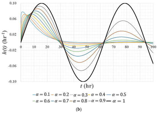
Figure 1.
Impulse response function of fractional linear reservoir model: (a) ; (b) .
One can readily see that Figure 1b, for , would be unsuitable for an impulse response function of a hydrologic system due to the presence of oscillations, even including the negative values of . In fact, this kind of unrealistic behavior of has already been reported in previous research, and it is mainly associated with the determination of an optimal IUH in the framework of a linear time-invariant hydrologic system [34,35]. Traditionally, it has been treated as an undesirable byproduct attributed to observational errors in hydrologic practice. In this regard, Figure 1b could provide new insight into the long-standing hydrologic problems related to the emergence of IUH with negative values.
In contrast to Figure 1b, ref. [36] proves Figure 1a, for , to be a PDF following the so-called Mittag–Leffler distribution [37,38]. In hydrology, an IUH is regarded as a PDF of water particles’ travel time to the outlet of a river basin [39]. So, Figure 1a can be thought of as a variety of IUHs emerging from the single linear reservoir model with constant but varying . In this figure, the black bold curve depicts for , which is equivalent to an impulse response function of a linear reservoir model in Equation (5). It is clearly seen that the remaining curves of for various vary faster with time in the vicinity of the origin but slower in the tail part, in comparison with the black bold one. So, we can expect that a fractional linear reservoir model could produce the impulse response functions in a nonlinear nature, which is characterized by a different rate of variation with time subject to compared to a linear reservoir model.
3.2. Unit Pulse Response Function
Letting in Equation (1) be the unit step function , in Equation (1) corresponds to an S hydrograph , which is generally used in hydrology [40]. Therefore, of a linear reservoir model can come from integrating Equation (5)
Referencing the first term on the right-hand side of Equation (13), the of a fractional linear reservoir model can be expressed in the form of Laplace transforms
where denotes the Laplace transform of , which can be inversely transformed with the help of Equation (10)
when Equation (17) is converted into Equation (15) [28]. So, the unit pulse response function of both linear reservoir models, , can be formulated by using Equations (15) and (17)
Equation (18) can be seen equivalent to the duration unit hydrograph with the finite rainfall duration of [40]. So, we can expect that given an effective rainfall hyetograph , a direct runoff hydrograph can be estimated by using a discrete convolution of with in the exact same way as unit hydrographs
where , so that and are indices for discrete time steps with being the total rainfall duration.
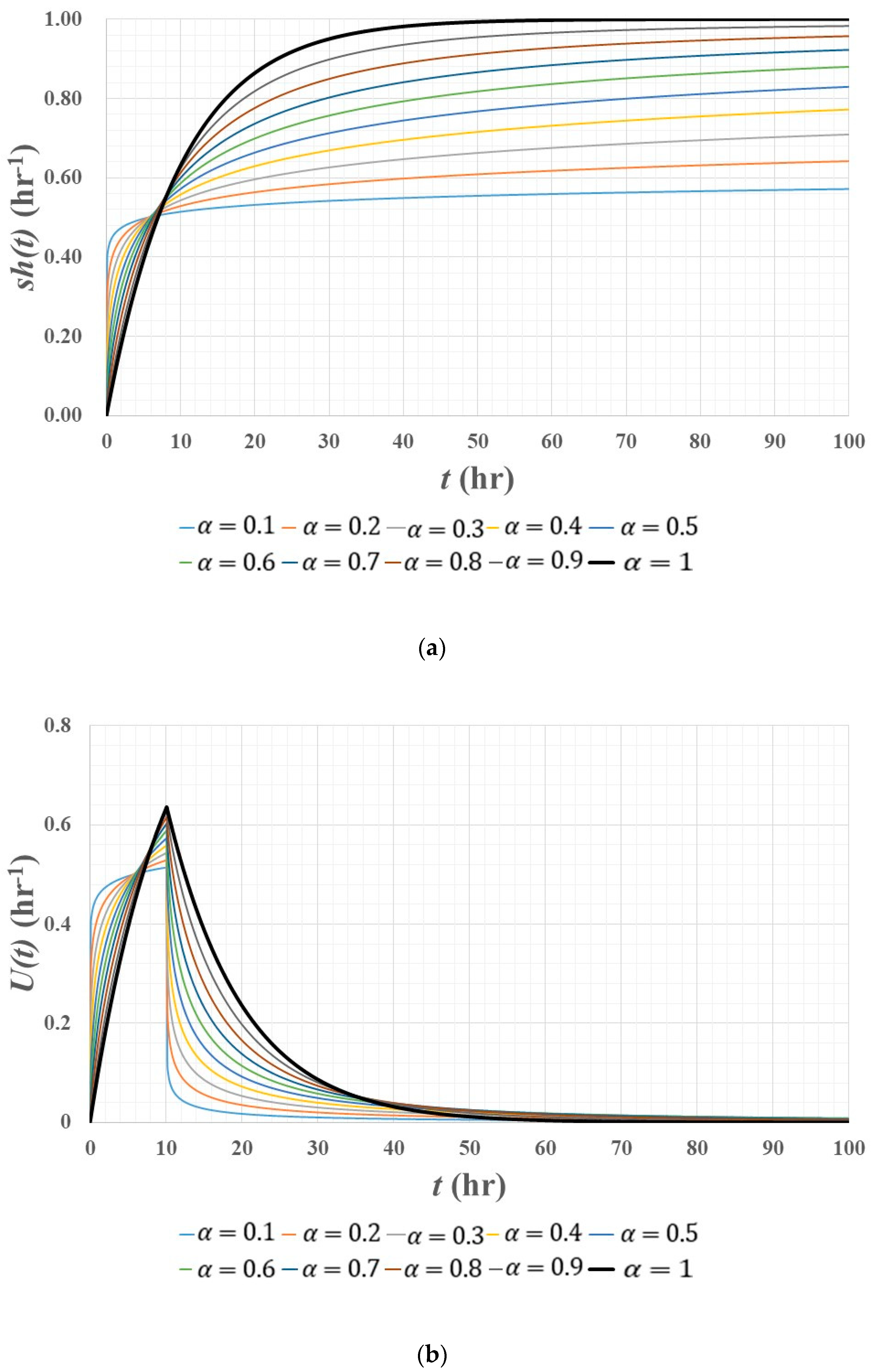
Figure 2 illustrates various and for , which are relevant to the PDF of the Mittag–Leffler distribution depicted in Figure 1a. Despite the traditional assumption of a finite base time of unit hydrographs [2], the base time of is theoretically infinite. So, it has been practically approximated as the time in which the value of closely approaches unity within the allowable tolerance (for instance, in HEC-1). In this respect, Figure 2a implies that the base time of could grow extremely long depending on In this figure, for (the black bold curve) already arrives nearby the value of unity at the lapsed time of about , whereas the remaining ones do not reach the unity value within the time span of . The long span of the base time for direct runoff hydrographs often happens in the separation procedure of total runoff hydrographs when using a straight line. To avoid this, several methods have been recommended for base flow separation, such as the fixed base method and variable slope method in the hydrologic literature [40]. However, they are known to be empirical ones and, furthermore, there is no evidence to guarantee that they are free of subjectivity in determining the cease point of direct runoff on recession curves. Rather, we can say that the straight line method could yield the most objective estimate of base flow, although it is the simplest among the others. So, if allowing the validity of the straight line method, Figure 2a implies that it could be possible for the span of base time to be much longer than the commonly acknowledged one in hydrologic practice. This might also be reminiscent of the old water paradox [41] in which the extremely long travel time of water particles to the outlet is reported within the framework of isotope hydrology.

Figure 2.
Hydrologic response function of the fractional linear reservoir model: (a) unit step re-sponse function, (b) unit pulse response function.
4. Results and Discussions
4.1. Methodology
In order to test the applicability of a fractional linear reservoir model to rainfall–runoff modeling at the simplest level, we picked an illustrative example problem concerned with the storage function method from the textbook of hydrology in Korea [42]. The storage function method is the most frequently used rainfall–runoff model in the hydrologic practice of Korean water management, which can be written by a continuity equation and a nonlinear storage relationship
where is a basin lag time, with being an exponent that specifies a nonlinear relation of to . Therefore, this model could be viewed as a kind of lag and route model [43]. However, unlike the traditional lag and route model, the storage function method does not lend itself to an explicit form of a response function to rainfall due to Equation (21), so a finite difference scheme has been used for routing of a nonlinear reservoir
where the subscript stands for an index of discrete time steps () with denoting . To take account into the initial loss of rainfall, the storage function method is equipped with the saturation rainfall and runoff ratio , by which total drainage area of is divided into the runoff area () and the percolation area (). Through Equation (22), is estimated only over the runoff area until total rainfall arrives at , while for both areas after total rainfall arrives at . Additionally, then, two runoff components are summed to each other. So, a total of five parameters is required to perform the storage function method.
Similar to the storage function method, we extend a linear reservoir model in Equation (5) as well as a fractional linear reservoir model in Equation (14) to lag and route versions in Table 1. It is noted that the former, in the same form as the traditional lag and route model, has two parameters of and , whereas the latter three parameters of , , and . For the sake of simplicity, we adopt the same as the one used in the storage function method to both of models in lag and route versions. Then, we estimated the remaining parameters based on the golden section search method to minimize the sum of the squared errors by using the rainfall–runoff data in the example problem.

Table 1.
Lag and route versions of linear reservoir models.
4.2. Results
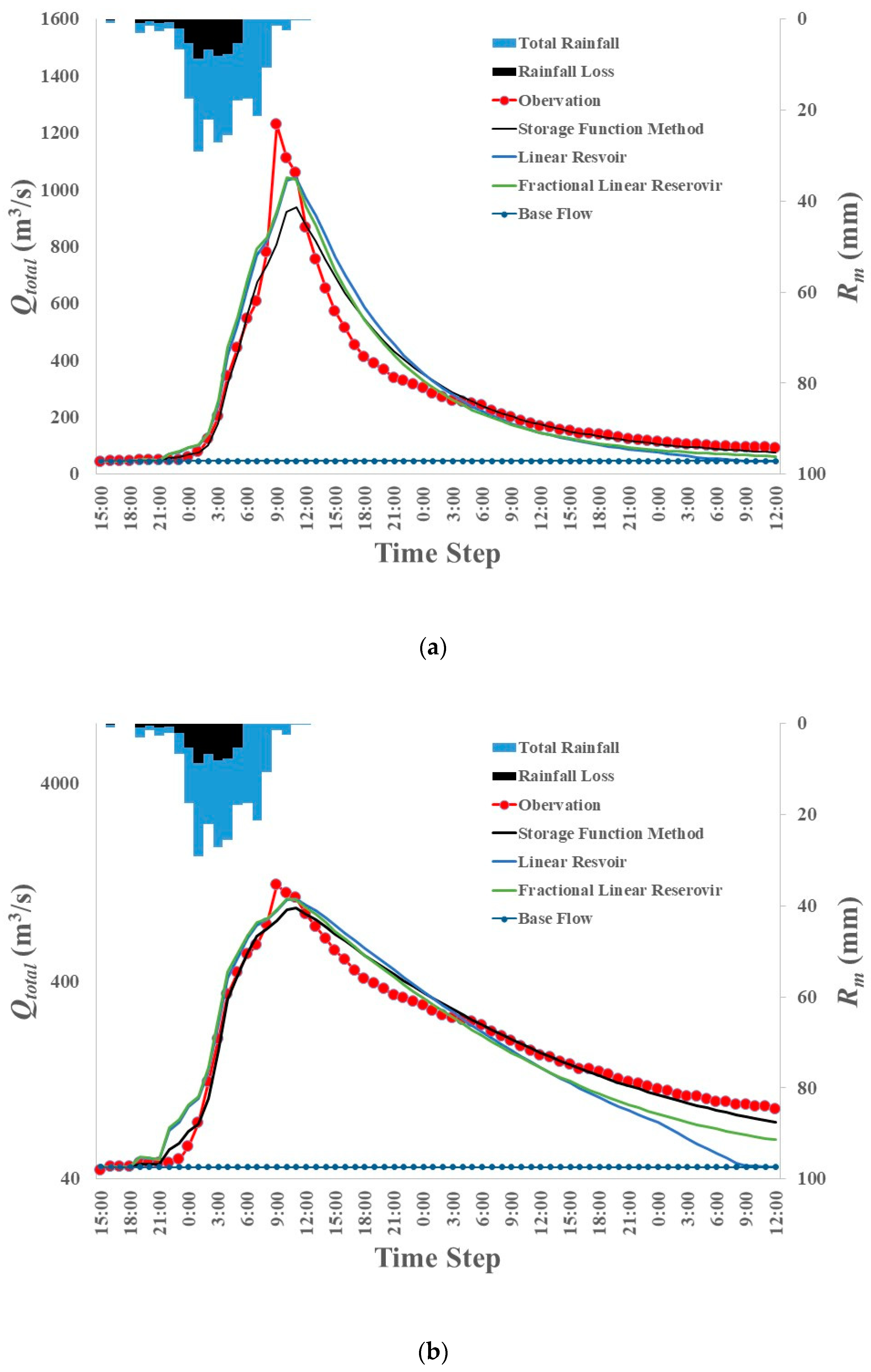
Figure 3 depicts an overview of the rainfall–runoff event in the example problem considered in this study, which has been originally designed to demonstrate the performance of the storage function method concerning the river basin with a drainage area of [42]. In this figure, the red curve with circles represents the observation of total runoff hydrographs while the black one is coming from the storage function method with the prescribed parameters for the demonstration; , , , , and [42]. It is noted that the base flow, the deep blue curve with circles, is separated from the observation by means of a straight line.
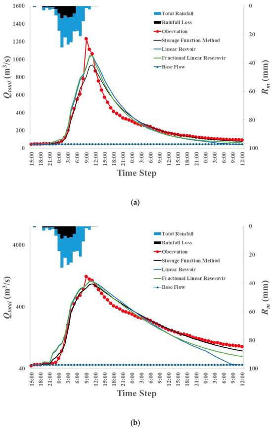
Figure 3.
Overview of rainfall–runoff event: (a) in normal scale, (b) in logarithmic scale.
Table 2 lists the estimated parameters of two lag and route models presented in Table 1, in which the values in parenthesis of the third column come from the multi-dimensional golden section search method recently suggested by [44]. In fact, the golden section search method has been originally developed to solve the one-dimensional search problems; therefore, we estimate (the value in the second column of Table 2) for the lag and route version of a linear reservoir model with the same , such as the one used in the storage function method in the first step. Then, we successively estimated (the value outside of parenthesis in the third column of Table 2) for the lag and route version of a fractional linear reservoir model with the same and as the previous step through the golden section search method again in the second step. We use in a dimension of following Equation (19) in the first step, in which denotes the discrete counterpart of with being the base time of direct runoff. However, in the second step, we use in a dimension of 30,000. This is intended to guarantee that every for any value of within the search interval approaches at least 0.99 at each iteration procedure. Then, we applied the multi-dimensional golden section search method [44] to the lag and route version of a fractional linear reservoir model with in a dimension of 30,000 in order to validate the estimates from the previous successive search procedures. Comparing two parameter sets for a fractional linear reservoir model in the third column of Table 2, a significant difference between them cannot be found. Therefore, we choose the parameter set coming from the successive estimation processes with the one-dimensional golden section search method mentioned above.
Table 2.
Results of parameter estimation for lag and route models.
It can be seen in Figure 3a that all three models tend to underestimate peak discharges relative to the observed one. Generally, the convolution operation in Equation (19) is well known to unduly attenuate input signals, so the lower peak discharges of the computed hydrographs in Figure 3 might be due to the routing procedure operated in the lag and route models used in this study. However, it is noted that two lag and route models based on linear and fractional linear reservoirs seem to be more suitable in terms of rainfall than the storage function method in that the formers produce faster-rising limb and closer peak discharge to the observation than the latter. So, we could expect that the models based on linear and fractional linear reservoirs could better reflect rainfall variations in the rising limb of runoff hydrographs than those based on a nonlinear reservoir.
In contrast, rather different features can be found in terms of the recession limb in Figure 3b, which is depicted on semi-logarithmic paper. In this figure, the storage function method produces recession curve that is more similar to the observation than the remaining two models. Nevertheless, it is also noted that the recession curve from a linear reservoir model reduces the base flow swiftly, whereas a fractional linear reservoir model makes a slower drawdown of the recession curve along with the trajectory of the red curve with circles despite the lesser magnitude of discharge than the observation.
In summary, a linear reservoir model would quickly respond to rainfall in both rising and recession periods of runoff processes while more slowly to a nonlinear reservoir in both periods. However, a fractional linear reservoir model shows a mixed behavior with fast-rising and slow-recession, so it might be located somewhere between a purely linear reservoir and purely nonlinear reservoir models. It is interesting that though a fractional linear reservoir model is operated in the same framework of the linear hydrologic system through Equation (19), it can effectively produce the nonlinear property of runoff processes.
Table 3 details the mean biased error (MBE) and the root mean squared error (RMSE) of the three calculated hydrographs compared to the observation, as shown in Figure 3. It is noted that the fractional linear reservoir model could produce a comparable result to that of the storage function method, also showing a slightly better performance than the linear reservoir model.
Table 3.
MBE and RMSE for lag and route models.
4.3. Discussions
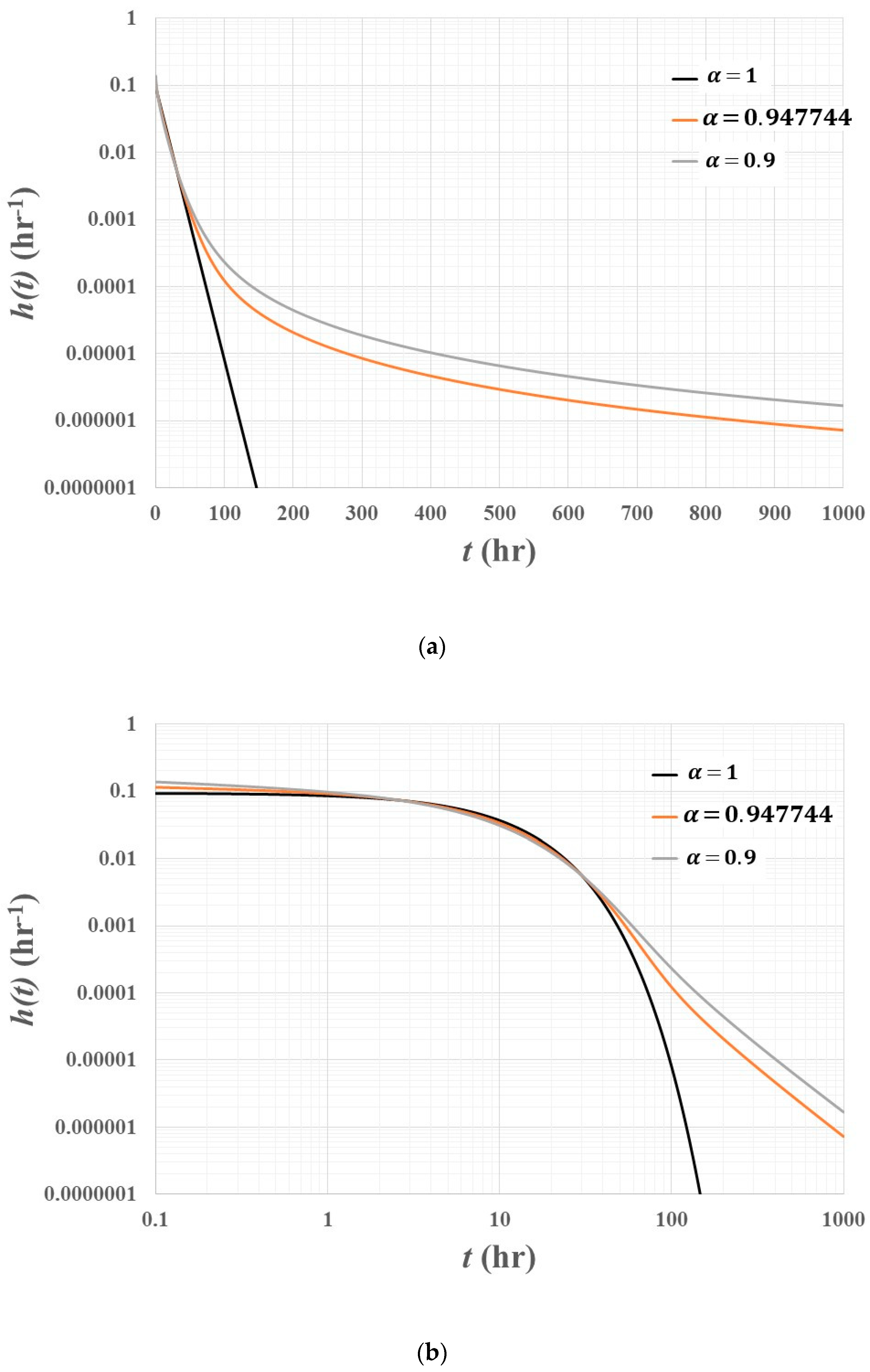
Figure 4 shows , which was removed from the translation effect due to for the basin of interest, which is considered in the example problem. It is superposed by for and . Figure 4a is described on semi-logarithmic paper, while Figure 4b is described on double-logarithmic paper. In Figure 4a, the curve in black represents for , the analytical solution to the linear reservoir model in Equation (5) for the basin of interest. This curve seems to be in a linear form on semi-logarithmic paper due to the exponential function in Equation (5). Therefore, we can think that the curvilinear behavior of the remaining two curves would indicate the nonlinear property of a fractional linear reservoir model, as mentioned in Section 3.1. It can be clearly observed that these two curves increasingly deviate from the black one as time proceeds, so the nonlinearity of those tends to be more profound with time. In [45], the equivalence of the fractional relaxation equations to differential equations with time-varying coefficients is shown. In this context, the deviations of two curves from the black one in Figure 4a could be attributed to the time-varying feature of the proportional constant of a linear reservoir model, which is usually interpreted as the mean residence time. In this regard, ref. [46] estimates as follows by applying geomorphologic IUH theory based on a linear reservoir model
where is the geomorphologic characteristic path length of a river basin, with being the average flow velocity. Equation (23) implies that the time-variant property of might come from the variation of . According to the saturation excess overland flow mechanism [47], it could be reasonable to assume overland flow with relatively faster , which occurs within the lower region around the channel networks in a river basin, can likely govern the whole runoff process in the vicinity of the origin of Figure 4a. However, as time goes on, the water particles undergoing the subsurface runoff, characterized by a relatively slower , could have a greater contribution to the runoff process in the tail part of Figure 4a. Therefore, the different origins of runoff generation could result in the time-variant property of characterized by time-varying , as depicted in Figure 4a. Based on the results above, we could say that a fractional linear reservoir model has the potential to reflect the nonlinear property of rainfall–runoff phenomena through its time-variant characteristics owing to the heterogeneous movement of water particles. In this respect, can be viewed as a kind of parameter to quantify the heterogeneity of runoff generation within a whole river basin.
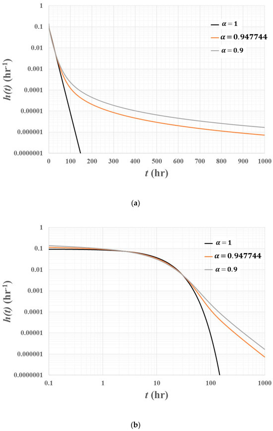
Figure 4.
IUH of fractional linear reservoir model for the basin of interest: (a) semi-logarithmic scale; (b) double-logarithmic scale.
Figure 4b clearly depicts the time-variant property of with two distinct distributional features. In this figure, the black curve represents for , which is the same as that shown in Figure 4a; the remaining two curves show a similar shape to the exponential distribution (the black curve) in the vicinity of the origin, whereas a similar shape to the power law distribution is evident in the tail part. Therefore, we can think that, in a fractional linear reservoir model, the travel time distribution of water particles to the outlet tends to follow an exponential distribution initially but follows a power law distribution later. Generally, the power law distribution implies scale invariance within the extremely long range of random variables; therefore, their statistical moments cannot be defined [48]. This is parallel with the infinite characteristic time of transfer functions, as shown in [13]. So, by allowing for the possibility of the long span of base times depicted in Figure 2a, a much wider time window would be required to separate the rainfall–runoff event from the continuous observation records in the context of a fractional linear reservoir model.
5. Conclusions
The following are the noteworthy results of this study.
- (1)
- The impulse response function of a fractional linear reservoir model has a nonlinear nature, which can be characterized by different rates of variation in terms of time.
- (2)
- The lag and route versions of fractional linear reservoir models produce the fast-rising and slow-recession of runoff hydrographs, that is, the mixed response of linear and nonlinear reservoir models to rainfall. So, a fractional linear reservoir model could be considered to be an effective tool in terms of reflecting the nonlinearity of rainfall–runoff phenomena within the framework of linear hydrologic system theory.
- (3)
- The fractional order, specifying a fractional linear reservoir model, can be viewed as a kind of parameter to quantify the heterogeneity of runoff generation within a river basin.
- (4)
- It could be possible for the span of base time to be much longer than that commonly acknowledged in hydrological practice, so a much wider time window would be required to separate the rainfall–runoff event from the continuous observation records in the context of a fractional linear reservoir model.
Author Contributions
Conceptualization, Y.-J.Y. and J.-C.K.; methodology, J.-C.K.; software, J.-C.K.; validation, Y.-J.Y. and J.-C.K.; formal analysis, Y.-J.Y. and J.-C.K.; investigation, Y.-J.Y. and J.-C.K.; resources, J.-C.K.; data curation, J.-C.K.; writing—original draft preparation, J.-C.K.; writing—review and editing, Y.-J.Y. and J.-C.K.; visualization, J.-C.K.; supervision, Y.-J.Y. and J.-C.K.; project administration, Y.-J.Y. and J.-C.K.; funding acquisition, Y.-J.Y. and J.-C.K. All authors have read and agreed to the published version of the manuscript.
Funding
This research was funded by the Konyang University Research Fund in 2023 and the National Research Foundation of Korea (NRF), grant number NRF-2022R1I1A1A01056269.
Data Availability Statement
Data available on request due to restrictions eg privacy or ethical.
Acknowledgments
The author, Joo-Cheol Kim, sincerely thanks Hyouna Lim for her heartful support.
Conflicts of Interest
The authors declare no conflict of interest.
References
- Amorocho, J. The nonlinear prediction problem in the study of the runoff cycle. Water Resour. Res. 1967, 3, 861–880. [Google Scholar] [CrossRef]
- Sherman, L.K. Streamflow from rainfall by the unit-graph method. Eng. News Record 1932, 108, 501–505. [Google Scholar]
- Zoch, R.T. On the relation between rainfall and stream flow. Mon. Weather Rev. 1934, 62, 315–322. [Google Scholar] [CrossRef]
- Kimura, T. The Flood Runoff Analysis Method by the Storage Function Model; The Public Works Research Institute, Ministry of Construction: Tsukuba, Japan, 1961.
- La Barbera, P.; Rosso, R. On the Fractal dimension of stream networks. Water Resour. Res. 1989, 25, 735–741. [Google Scholar] [CrossRef]
- Rosso, R.; Bacchi, B.; La Barbera, P. Fractal relation of mainstream length to catchment area in river networks. Water Resour. Res. 1991, 27, 381–387. [Google Scholar] [CrossRef]
- Tarboton, D.G.; Bras, R.L.; Rodriguez-Iturbe, I. The Fractal nature of river networks. Water Resour. Res. 1988, 24, 1317–1322. [Google Scholar] [CrossRef]
- Hilfer, R. Applications of Fractional Calculus in Physics; World Scientific: Singapore, 2000. [Google Scholar]
- Kulish, V.V.; Lage, J.L. Application of fractional calculus to fluid mechanics. J. Fluids Eng. 2002, 124, 803–806. [Google Scholar] [CrossRef]
- Dalir, M.; Bashour, M. Applications of fractional calculus. Appl. Math. Sci. 2010, 4, 1021–1032. [Google Scholar]
- Tarasov, V.E. On history of mathematical economics: Application of fractional calculus. Mathematics 2019, 7, 509. [Google Scholar] [CrossRef]
- Benson, D.A.; Meerschaert, M.M.; Revielle, J. Fractional calculus in hydrologic modeling: A numerical perspective. Adv. Water Resour. 2013, 51, 479–497. [Google Scholar] [CrossRef]
- Guinot, V.; Savéan, M.; Jourde, H.; Neppel, L. Conceptual rainfall–runoff model with a two-parameter, infinite characteristic time transfer function. Hydrol. Process. 2015, 29, 4756–4778. [Google Scholar] [CrossRef]
- Kavvas, M.L.; Ercan, A. Fractional governing equations of diffusion wave and kinematic wave open-channel flow in fractional time-space. I. Development of the equations. J. Hydrol. Eng. 2015, 20, 04014096. [Google Scholar] [CrossRef]
- Su, N.; Zhang, F. Anomalous overland flow on hillslopes: A fractional kinematic wave model, its solutions and verification with data from laboratory observations. J. Hydrol. 2022, 604, 127202. [Google Scholar] [CrossRef]
- Unami, K.; Fadhil, R.M.; Mohawesh, O. Bounding linear rainfall-runoff models with fractional derivatives applied to a barren catchment of the Jordan Rift Valley. J. Hydrol. 2021, 593, 125879. [Google Scholar] [CrossRef]
- Wheatcraft, S.W.; Meerschaert, M.M. Fractional conservation of mass. Adv. Water Resour. 2008, 31, 1377–1381. [Google Scholar] [CrossRef]
- Xiang, X.; Ao, T.; Li, X. Application of a Fractional Instantaneous Unit Hydrograph in the TOPMODEL: A Case Study in Chengcun Basin, China. Appl. Sci. 2023, 13, 2245. [Google Scholar] [CrossRef]
- Borthwick, M.F. Application of Fractional Calculus to Rainfall Streamflow Modelling. Ph.D. Dissertation, University of Plymouth, Plymouth, UK, 2010. [Google Scholar]
- Chow, V.T.; Kulandaiswamy, V.C. General hydrologic system model. J. Hydraul. Div. 1971, 97, 791–804. [Google Scholar] [CrossRef]
- Dooge, J.C.I. A general theory of the unit hydrograph. J. Geophys. Res. 1959, 64, 241–256. [Google Scholar] [CrossRef]
- Nash, J.E. The form of the instantaneous unit hydrograph. Comptes Rendus Rapp. Assem. Gen. Tor. 1957, 3, 114–121. [Google Scholar]
- Singh, K.P. Nonlinear instantaneous unit hydrograph theory. J. Hydraul. Div. 1964, 90, 313–347. [Google Scholar] [CrossRef]
- Kisela, T. Fractional Differential Equations and Their Applications. Ph.D. Thesis, BRNO University of Technology, Brno, Czech Republic, 2008. [Google Scholar]
- Caputo, M. Linear models of dissipation whose Q is almost frequency independent—II. Geophys. J. Int. 1967, 13, 529–539. [Google Scholar] [CrossRef]
- Caputo, M.; Fabrizio, M. A new definition of fractional derivative without singular kernel. Prog. Fract. Differ. Appl. 2015, 1, 73–85. [Google Scholar]
- Atangana, A.; Baleanu, D. New fractional derivatives with nonlocal and non-singular kernel: Theory and application to heat transfer model. Therm. Sci. 2016, 20, 763–769. [Google Scholar] [CrossRef]
- Podlubny, I. Fractional Differential Equations; Academic Press: Cambridge, MA, USA, 1999. [Google Scholar]
- Haubold, H.J.; Mathai, A.M.; Saxena, R.K. Mittag-Leffler functions and their applications. J. Appl. Math. 2011, 2011, 298628. [Google Scholar] [CrossRef]
- Mainardi, F. Why the Mittag-Leffler function can be considered the Queen function of the Fractional Calculus? Entropy 2020, 22, 1359. [Google Scholar] [CrossRef] [PubMed]
- Dooge, J.C.I. Linear Theory of Hydrologic Systems; Agricultural Research Service, US Department of Agriculture: Washington, DC, USA, 1973.
- Singh, V.P. Hydrologic Systems: Rainfall-Runoff Modeling; Prentice Hall: Upper Saddle River, NJ, USA, 1988. [Google Scholar]
- Garrappa, R. The Mittag-Leffler Function. Available online: https://www.mathworks.com/matlabcentral/fileexchange/48154-the-mittag-leffler-functionMATLABFileExchange (accessed on 2 January 2023).
- Diskin, M.H.; Boneh, A. Determination of an optimal IUH for linear, time invariant systems from multi-storm records. J. Hydrol. 1975, 24, 57–76. [Google Scholar] [CrossRef]
- Kwon, O.H.; Ryu, T.S.; Yoo, J.H. A derivation of the representative unit hydrograph from multiperiod complex storm by linear programming. KSCE J. Civ. Environ. Eng. Res. 1993, 13, 173–182. (In Korean) [Google Scholar]
- Pillai, R.N. On Mittag-Leffler functions and related distributions. Ann. Inst. Stat. Math. 1990, 42, 157–161. [Google Scholar] [CrossRef]
- Cahoy, D.O. Estimation of Mittag-Leffler parameters. Commun. Stat-Simul. C 2013, 42, 303–315. [Google Scholar] [CrossRef]
- Cahoy, D.O.; Polito, F. Renewal processes based on generalized Mittag–Leffler waiting times. Commun. Nonlinear Sci. Numer. Simul. 2013, 18, 639–650. [Google Scholar] [CrossRef]
- Rodríguez-Iturbe, I.; Valdés, J.B. The geomorphologic structure of hydrologic response. Water Resour. Res. 1979, 15, 1409–1420. [Google Scholar] [CrossRef]
- Chow, V.T. Applied Hydrology; McGraw Hill: New York, NY, USA, 1988. [Google Scholar]
- Botter, G.; Bertuzzo, E.; Rinaldo, A. Transport in the hydrologic response: Travel time distributions, soil moisture dynamics, and the old water paradox. Water Resour. Res. 2010, 46, W03514. [Google Scholar] [CrossRef]
- Yoon, Y.N. Hydrology: Basics and Applications; Cheongmungak: Seoul, Republic of Korea, 2007. (In Korean) [Google Scholar]
- Wang, G.T.; Wu, K. The unit-step function response for several hydrological conceptual models. J. Hydrol. 1983, 62, 119–128. [Google Scholar] [CrossRef]
- Rani, G.S.; Jayan, S.; Nagaraja, K.V. An extension of golden section algorithm for n-variable functions with MATLAB code. IOP Conf. Ser. Mater. Sci. Eng. 2019, 577, 012175. [Google Scholar] [CrossRef]
- Mainardi, F. A note on the equivalence of fractional relaxation equations to differential equations with varying coefficients. Mathematics 2018, 6, 8. [Google Scholar] [CrossRef]
- Cheng, B.L.M. A Study of Geomorphologic Instantaneous Unit Hydrograph. Ph.D. Thesis, University of Illinois, Champaign, IL, USA, 1982. [Google Scholar]
- Dunne, T.; Black, R.D. Partial area contributions to storm runoff in a small New England watershed. Water Resour. Res. 1970, 6, 1296–1311. [Google Scholar] [CrossRef]
- Newman, M.E.J. Power laws, Pareto distributions and Zipf’s law. Contemp. Phys. 2005, 46, 323–351. [Google Scholar] [CrossRef]

Disclaimer/Publisher’s Note: The statements, opinions and data contained in all publications are solely those of the individual author(s) and contributor(s) and not of MDPI and/or the editor(s). MDPI and/or the editor(s) disclaim responsibility for any injury to people or property resulting from any ideas, methods, instructions or products referred to in the content. |
© 2023 by the authors. Licensee MDPI, Basel, Switzerland. This article is an open access article distributed under the terms and conditions of the Creative Commons Attribution (CC BY) license (https://creativecommons.org/licenses/by/4.0/).