Article

A Stacking Ensemble Model of Various Machine Learning Models for Daily Runoff Forecasting

1
State Key Laboratory of Water Resources and Hydropower Engineering Science, Wuhan University, Wuhan 430072, China
2
Hubei Provincial Collaborative Innovation Center for Water Resources Security, Wuhan 430072, China
3
Information Centre, Ministry of Water Resources, Beijing 100053, China
4
Department of Water Resources of Hainan Province, Haikou 570100, China
*
Author to whom correspondence should be addressed.
Water 2023, 15(7), 1265; https://doi.org/10.3390/w15071265
Submission received: 2 March 2023 / Revised: 19 March 2023 / Accepted: 20 March 2023 / Published: 23 March 2023

Abstract

:
Improving the accuracy and stability of daily runoff prediction is crucial for effective water resource management and flood control. This study proposed a novel stacking ensemble learning model based on attention mechanism for the daily runoff prediction. The proposed model has a two-layer structure with the base model and the meta model. Three machine learning models, namely random forest (RF), adaptive boosting (AdaBoost), and extreme gradient boosting (XGB) are used as the base models. The attention mechanism is used as the meta model to integrate the output of the base model to obtain predictions. The proposed model is applied to predict the daily inflow to Fuchun River Reservoir in the Qiantang River basin. The results show that the proposed model outperforms the base models and other ensemble models in terms of prediction accuracy. Compared with the XGB and weighted averaging ensemble (WAE) models, the proposed model has a 10.22% and 8.54% increase in Nash–Sutcliffe efficiency (NSE), an 18.52% and 16.38% reduction in root mean square error (RMSE), a 28.17% and 18.66% reduction in mean absolute error (MAE), and a 4.54% and 4.19% increase in correlation coefficient (r). The proposed model significantly outperforms the base model and simple stacking model indicated by both the Friedman test and the Nemenyi test. Thus, the proposed model can produce reasonable and accurate prediction of the reservoir inflow, which is of great strategic significance and application value in formulating the rational allocation and optimal operation of water resources and improving the breadth and depth of hydrological forecasting integrated services.

1. Introduction

Runoff is a fundamental element of the hydrological cycle, and runoff prediction has thus been one of the fundamental issues in hydrology. Runoff is usually influenced by a combination of factors, such as precipitation, evaporation, solar radiation, and subsurface and atmospheric circulation, and shows high spatial and temporal variability and nonsmoothness. The impact of climate change and human activities has exacerbated the nonstationarity and nonconformity of runoff, leading to frequent extreme events such as droughts and floods, which have great impact on the socioeconomic and personal safety of residents. Enhancing accuracy in runoff forecasting is of great importance for water resources regulation [1], flood control [2], power generation [3], and others. In the current context of climate change and high human activity [4,5,6], runoff sequences exhibit volatility and randomness, which pose significant challenges for runoff prediction [7]. Therefore, it is necessary to search for more advanced runoff forecasting methods to provide higher accuracy and more stable runoff prediction [8].
In past decades, researchers have studied many methods and hydrological models to obtain accurate runoff predictions. These models can be divided into two categories: process-driven models and data-driven models [9,10]. Process-driven models, such as the Xin’anjiang model [11] and numerical weather prediction (NWP) [12,13], have a well-defined physical mechanism that simulates runoff based on the relationship between runoff and influencing factors. Process-based models utilize rainfall, topographic, and geological data as input parameters to forecast and simulate runoff through the development of intricate mathematical models. Therefore, accurate runoff process simulation requires a large number of hydrological data and fine underlying surface data [14]. Owing to the complexity of the hydrological cycle processes, process-driven model genesis is difficult and requires high computational costs. With the development of artificial intelligence and deep learning technology, data-driven models are more popular for runoff prediction at present. Data-driven models do not consider the physical mechanisms of hydrological processes and make forecasts directly by constructing a mapping relationship between forecast factors and runoff. These can be further partitioned into statistical models [15,16], machine learning models [17,18,19], and deep learning models [20,21]. Statistical models employ techniques to anticipate the progression of past runoff based on the temporal features of its time series. Autoregressive models (AR) [22], autoregressive moving average models (ARMA) [23], and autoregressive moving integrated average models (ARIMA) [24] have been widely applied for hydrological time series prediction. Nonetheless, these models are unable to adequately capture the intricate nonlinear correlations present in the runoff time series, thus leading to inferior model performance. Because of the limitations of time series models, various machine learning models and deep learning models have been applied to the prediction of nonlinear hydrological series in recent years. Yang et al. [9] employed random forest (RF), artificial neural network (ANN), and support vector regression (SVR) to predict one-month-ahead reservoir inflows and compared their capabilities. The results show that the prediction results obtained by RF have the best statistical performances compared with the other two methods, and RF can interpret raw model inputs. Liu et al. [25] were the first to apply the AdaBoost (adaptive boosting) ensemble technique to improve the efficiency of rainfall–runoff models. They reported that the enhanced AdaBoost model yielded more satisfactory results. Machine learning models have achieved substantial advancements in both predictive accuracy and effectiveness, and they are extensively employed in practical applications. Nevertheless, these models can be categorized as “shallow” learning approaches [26]. Xiang et al. [27] proposed a prediction model based on long short-term memory (LSTM) and sequence-to-sequence (seq2seq) structures and applied them to estimate hourly rainfall–runoff. The results show that the proposed model had sufficient predictive power and could be used to improve forecast accuracy in short-term flood forecast applications. Chen et al. [28] incorporated short previous time steps into LSTM and developed the self-attentive long short-term memory (SA-LSTM). The results show that SA-LSTM delivers superior performance relative to the most advanced benchmark models. From the above studies, it is clear that machine learning models perform well in nonlinear simulations in hydrology and are widely used in practical production.
Previous studies have generally performed simulated predictions based on individual machine learning models, showing their respective superiority. Although a single forecast model can improve the forecast accuracy by adjusting parameters and selecting forecast factors in the process of forecasting, the single model has model structure uncertainty and is difficult to adapt to different basins [29]. Numerous studies have shown that combining multiple single forecast models to build an ensemble forecast model can effectively exploit the advantages of different models and improve the reliability and accuracy of runoff forecasts [30,31,32,33]. Stacking is a popular ensemble learning technique that effectively mitigates bias and variance by combining weaker models to create a stronger one and has gained widespread use in the field of machine learning. Diks et al. [34] employed several method-averaging methods for runoff forecasting and found that Granger–Ramanathan averaging (GRA) was superior to other methods. Sun et al. [35] utilized the stacking ensemble learning method to predict the breakup dates of river ice. The results show that the combined models generally outperformed all member models. Nevertheless, the application of the stacking ensemble model for runoff prediction is still limited and there is much potential to be explored.
To further improve the accuracy of daily runoff prediction, a stacking ensemble model based on the attention mechanism called ATE is proposed in this study for daily runoff forecasting. The RF, AdaBoost, and XGB models were selected as the base models in the stacking model because they are representatives of the dominant ensemble models in runoff prediction. In addition, these three models they have complementary advantages and disadvantages that can be utilized in the stacking ensemble model. The improvement performance of the ATE model on runoff forecast accuracy is demonstrated by comparing the ATE model with common stacked models, such as simple average ensemble (SAE) and weighted average ensemble (WAE). The model performance evaluation indicators, such as root mean square error (RMSE), mean absolute error (MAE), correlation coefficient (r), and Nash–Sutcliffe efficiency (NSE), are used to compare and analyze the simulation results of the different models.

2. Methodology

2.1. Machine Learning Methods

2.1.1. Random Forest (RF)

Random forest (RF) is an ensemble learning method based on the aggregation of decision trees for classification or regression prediction. The first algorithm for random forest was created by Ho [36] and was then developed by Breiman [37]. It has been widely used in many applications such as rainfall forecasting [38], land cover classification [39], sensitivity analysis [40], and solar radiation forecasting [41]. RF is a popular machine learning tool that uses the bootstrap resampling method to extract multiple random subsets from the training data, model the decision tree for each bootstrap subset, and then combine the prediction results of multiple decision trees to average the final regression or classification prediction results [42]. RF solves the problem of decision-tree performance bottleneck, has good tolerance to noise and outliers, and has good scalability and parallelism for high-dimensional data classification problems. RF can handle very large amounts of data, and the so-called “dimensionality disaster” in big data often makes other models fail. At the same time, it has almost the same error rate as any other method for most learning tasks and has less tendency to overfit. RF is one of the best-known bagging algorithms and has good performance in regression problems, so it was chosen as one of the base models for the ensemble model in this study.

2.1.2. Adaptive Boosting

The AdaBoost algorithm, also known as adaptive boosting, was first introduced as an iterative boosting-ensemble machine learning algorithm by Freund and Schapire [43]. The principle of the AdaBoost algorithm is to train different learners (weak learners) with the same training set, and then aggregate these weak learners to form stronger learners [44]. The algorithm divides the sample set into several parts and assigns the dataset to the base learner for training according to the weight size. The coefficients of the base learners are adjusted by calculating the error, and then the weight distribution of the sample set is adjusted. After several iterations of training, all base learners are finally combined by weighting to build a strong learner. Moreover, AdaBoost is a simple boosting algorithm that can enhance the performance of weak learner algorithms. This algorithm is designed to improve the classification ability of the data by reducing both bias and variance through continuous training. In this study, AdaBoost was applied to boost the decision tree and construct one of the submodels of the ensemble model due to the fact that the AdaBoost algorithm has proven to be an effective and practical boosting algorithm.

2.1.3. Extreme Gradient Boosting (XGB)

Extreme gradient boosting (XGB), proposed by Chen and Guestrin [45], is an advanced supervised algorithm based on the gradient-enhanced decision tree. It has been employed in many different fields such as hydrology [46], remote sensing [47], and medicine [48]. The algorithm develops a “strong” learner by combining all the predictions of a set of “weak” learners through the additive training strategies. The algorithm is based on the gradient-boosted decision tree (GDBT) algorithm with a second-order Taylor expansion of the loss function and the addition of a regular term, which effectively avoids overfitting and accelerates the convergence speed. The XGB algorithm improves the prediction accuracy by continuously forming new decision trees to fit the residuals of previous predictions, so that the residuals between the predicted and true values are continuously reduced. XGB is the tool for the massively parallel boosting tree; it is currently the fastest and best open source boosting tree toolkit, more than 10 times faster than the common toolkit. Owing to XGB’s notable advantage over other gradient-boosting methods in terms of speed, it was chosen as one of the base models for the ensemble model in this study.

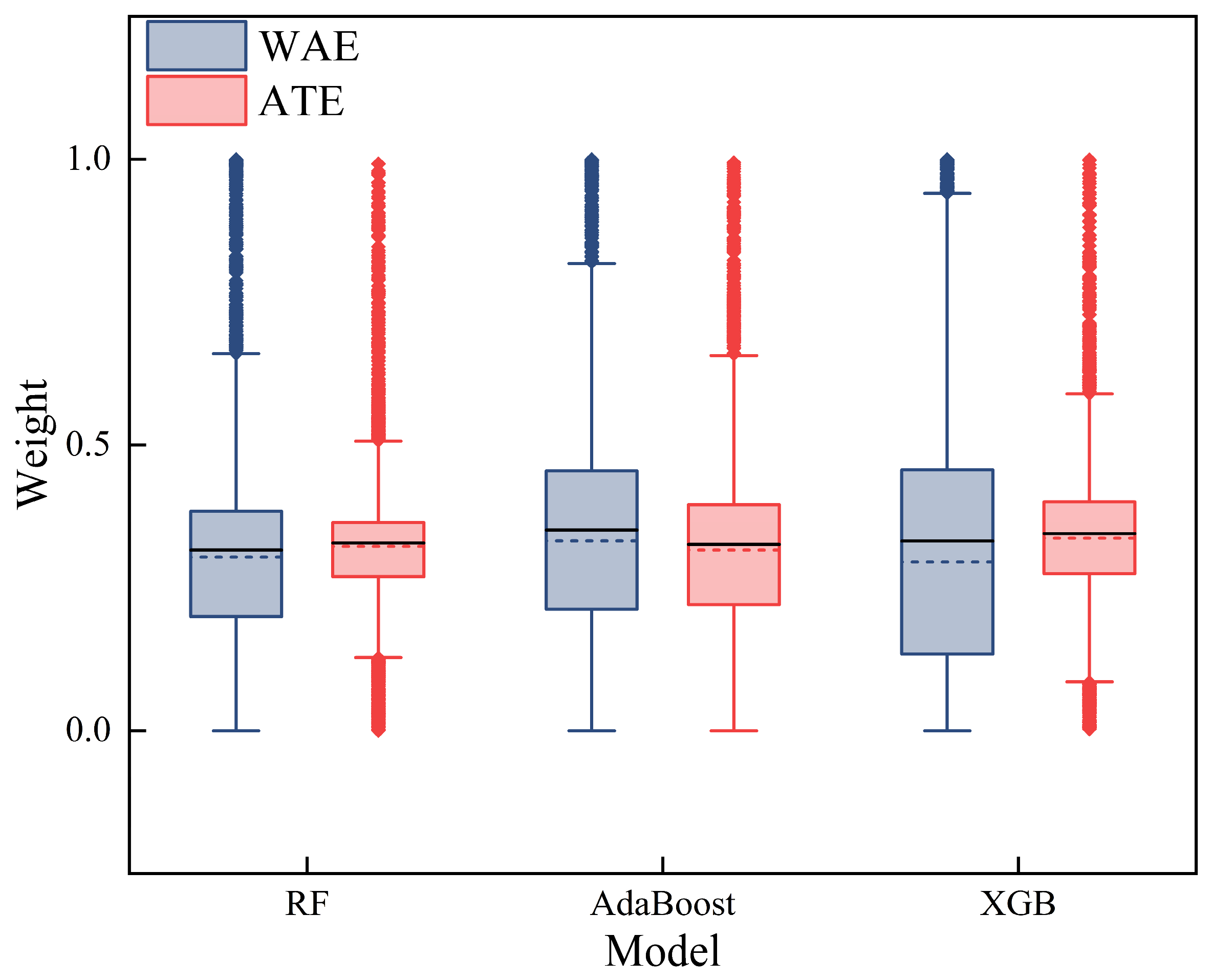
2.2. Proposed Stacking Ensemble Learning

Stacking ensemble learning refers to the methods that take advantage of mutual complementarity among the base models to improve performance and enhance generalization ability [49]. In general, stacking ensemble learning consists of two phases: base models training phase and meta model training phase [50]. In the first phase, the original data are divided into training set and testing set, and the training set is trained using the k-fold cross validation. The k-fold cross validation divides the training set into k pieces and each piece uses the remaining (k − 1) pieces of the data for training the model and simulating the predictions for that piece of the data. A diagram of the k-fold cross validation is shown in Figure 1. In the second phase, the predictions dataset obtained after the k-fold cross validation of the base model is reassembled, in the order of the original training dataset, to obtain a new training set. The training set of the meta model is obtained by merging the new training set of the multiple base models. Similarly, the predictions from the testing set of the base models are combined to obtain the testing set of the meta model. The meta model is trained based on the new dataset.
In stacking ensemble learning, the choice of base model and meta model is crucial. As mentioned above, three models, RF, AdaBoost, and XGB, were selected as the base models for the ensemble model in this study. Then, this study constructed an attention ensemble model (ATE) as the meta model based on the attention mechanism. The iterative training processes of the ATE model are as follows (Algorithm 1).
Algorithm 1 The iterative training process of the ATE model
Input: Training set D, Validation set D’, Attention-Based Stacking model.
Base models: Random Forest (RF), Adaptive Boosting (AdaBoost), Extreme Gradient Boosting (XGB)
Evaluation criteria: Nash–Sutcliffe Efficiency (NSE), Root Mean Squared Error (RMSE), Mean Absolute Error (MAE), Pearson Correlation Coefficient (r)
1: Initialize empty arrays F1 for predictions of base models on D’.
2: Initialize empty array P for actual values in D’.
3: For i = 1 to k do:
  a. Split D into D_train and D_val for training and validation, respectively, using k-fold cross-validation.
  b. Train base models on D_train.
  c. For each instance j in D_val do:
   i. Generate predictions pi1, pi2, pi3 using RF, AdaBoost, XGB, respectively.
   ii. Append pi1, pi2, pi3 to F1 for instance j.
   iii. Append actual value yj to P.
4: Train Attention-Based Stacking model on F1 as input and P as target.
5: Initialize empty arrays F2 and P2 for predictions of base models on D’ and actual values in D’, respectively.
6: For each instance i in D’, perform:
  a. Generate predictions pi1, pi2, pi3 using RF, AdaBoost, XGB, respectively.
  b. Append pi1, pi2, pi3 to F2 for instance i.
  c. Append actual value yi to P2.
7: Generate predictions p using F2 and Attention-Based Stacking model.
8: Calculate evaluation criteria NSE, RMSE, MAE, and r using p and P2.
9: Repeat steps 3–8 for k-fold cross-validation and report average evaluation criteria.
10: Train final Attention-Based Stacking model on D using all instances.
11: Save the final model for future use.
The general flow chart of the construction of the proposed attention ensemble model in this study is shown in Figure 2.
In addition to the attention ensemble learning, the study applied the simple averaging ensemble and the weighted averaging ensemble set as comparison methods.
The simple averaging ensemble (SAE) model is founded on the principle of the arithmetic mean. Suppose there are K base models in an ensemble model; the SAE model’s output can be defined as
f SAE ( x ) = 1 K k = 1 K f i ( x )   ,     x = 1 , 2 , , N .
where f i ( x ) is the output of the kth base model and N denotes the length of the dataset.
As can be seen above, in the SAE model, the weights of the predicted values of each base model are the same, which does not sufficiently consider the forecast variability of each model. The weighted averaging ensemble (WAE) model is based on the difference in the prediction accuracy of each base model, and the predictions are combined to improve the accuracy of the ensemble model. The output of the WAE model can be defined as
f WAE ( x ) = k = 1 K ω i f i ( x )   ,     x = 1 , 2 , , N .
where ω i ( x ) is the weight of the kth base model when the input is x, and N denotes the length of the dataset. The ω i ( x ) is determined by the following steps: first, find the sum of squared dispersions of the predicted values of each base model, and then find the corresponding weights of each model using Equation (3). The weight can be calculated as
ω i ( x ) = D k 1 ( x ) k = 1 K D k 1 ( x )
where D k ( x ) is the square of the deviation of the kth model prediction.

2.3. Hyper-Parameter Optimization

In machine learning, hyper-parameters need to be set in advance before the model is trained. For the RF, AdaBoost, and XGB algorithms, hyper-parameters have a significant effect on the prediction accuracy of the model. Therefore, hyper-parameter optimization is of great importance. The main strategies in the current optimization of hyper-parameters are babysitting, grid search, random search, and Bayesian optimization [51]. Compared to the other three strategies, Bayesian optimization is more generalizable over the test set and requires fewer iterations, so it was utilized for fine-tuning the hyper-parameters for the models employed in this study.
The hyper-parameters for the models are tuned and evaluated over the training dataset using the Hyperopt library in Python combined with k-fold cross-validation. The specific steps are as follows:
Step 1:
Define the objective function. Define an objective function with the hyper-parameters as inputs and the MSE as the model performance evaluation metric, and use k-fold cross-validation to calculate the generalization error for each set of hyper-parameters over k models, and apply its average as the output.
Step 2:
Define the hyper-parameter space. A preliminary determination of the search space of hyper-parameters was determined based on practical experiences of previous research.
Step 3:
Define the hyper-parameter optimization algorithm. The tree-structured Parzen estimator algorithm was chosen to search the hyper-parameter space.
Step 4:
Run hyper-parameter optimization. The ”fmin” function was chosen to run the hyper-parameter optimization and set the maximum number of iterations to 1000 to finally obtain the optimal hyper-parameters for the model.
Table 1 presents a compendium of the main hyper-parameters for the three machine learning models utilized in this study.

2.4. Model Performance Evaluation

When evaluating the predictive capacity of developed models, it is crucial to employ a diverse range of metrics to measure errors. To compare the performance of the models, the root mean square error (RMSE), the mean absolute error (MAE), the correlation coefficient (r), and the Nash–Sutcliffe efficiency (NSE) were applied in this study. NSE can be effective in evaluating the accuracy and stability of model forecast results, and r can help evaluate the linear correlation of forecast results. RMSE and MAE are two of the most commonly used metrics for measuring the accuracy of model predictions. RMSE measures the average magnitude of the errors in the predictions, and is particularly sensitive to large errors. MAE measures the average absolute magnitude of the errors, and is generally less sensitive to outliers than RMSE. By using these four criteria, the performance of the model can be evaluated in different ways, considering both the accuracy and the fit of the model. The formulae for the four evaluation criteria are as follows:
RMSE = 1 N i = 1 N ( y P , i y O , i ) 2
MAE = 1 N i = 1 N y P , i y O , i
r = i = 1 N ( y P , i y ¯ P , i ) ( y O , i y ¯ O , i ) i = 1 N ( y P , i y ¯ P , i ) 2 i = 1 N ( y O , i y ¯ O , i ) 2
NSE = 1 i = 1 N ( y P , i y O , i ) 2 i = 1 N ( y O , i y ¯ O , i ) 2
where y O , i and y P , i are the observed and predicted runoff series, respectively; y ¯ O , i and y ¯ P , i are the mean values of the series y O , i and y P , i , respectively; and N is the number of data.

2.5. Significance Test for Model Performance Evaluation

In this study, the nonparametric Friedman test and Nemenyi test were mainly used to compare multiple models used in this study [52]. The main steps in the nonparametric Friedman test are summarized as follows:
Step 1:
The prediction results of N models on k folds are calculated. The prediction results in this study are assessed using the evaluation criteria of NSE, RMSE, MSE, and r.
Step 2:
For each fold, the tested models are ranked and given sequential values based on the merit of model performance of the prediction results.
Step 3:
Find the average (Ri) of N models ranked on all folds.
Step 4:
The Friedman test was used for comparison. The nonparametric Friedman statistic τχ2 is expressed as follows:
τ χ 2 = 12 k N N + 1 i = 1 N R i 2 N N + 1 2 4
In the nonparametric test, a p-value is used to determine the probability of rejecting the original hypothesis. A p-value < 0.05 indicates that the original hypothesis should be rejected, which indicates a statistically significant difference between the models.
If the results of the Friedman test indicate a “significant difference in model performance”, the post hoc Nemenyi test is required. The Nemenyi test process is as follows:
Step 1: Critical difference (CD) is calculated according to the following equation, where the critical values qα are 2.850 and 2.589 when the significance level is taken as 0.05 and 0.10, respectively.
CD = q α N ( N + 1 ) k
Step 2: The difference between the average rank difference (ARD) and CD of the two models is compared, and if ARD > CD, there is a significant difference in the performance of the two models.

3. Case Study

3.1. Study Area

The Fuchun River basin, located in the middle reaches of Qiantang River basin, was selected for this study. The Qiantang River basin is located in eastern China, which is one of the most economically developed regions in China. The basin has an area of about 55,600 km2 and is dominated by a subtropical humid monsoon climate, with abundant rainfall [53]. Influenced by typhoons and plum rains, flooding is frequent in the Qiantang River basin. In 2020, the Qiantang River basin suffered the strongest plum flood in history, and the water level of Xin’an River Reservoir reached the highest level in history, which greatly affected the socioeconomic and personal safety of residents. It is therefore of significant importance to implement more accurate and stable runoff forecasting for local water resource regulation and management.
For the daily runoff prediction, Fuchun River Reservoir (FCJ) located in the Fuchun River basin was selected. The catchment area of the Fuchun River basin is about 31,700 km2 and the total length of the main stream is 102 km. The average annual precipitation is approximately 1600 mm and the average temperature is 17.2 °C. Precipitation is mainly concentrated in the flood season from March to June, and the peak flow usually occurs during this period. Flow regulation in the Fuchun River basin is controlled by Xin’an River Reservoir (XAJ), located at the downstream end of the Xin’an River, and Fuchun River Reservoir (FCJ), located at the downstream end of the Fuchun River. Fuchun River Reservoir is a daily regulation type, with a total storage capacity of 920 million m3. The total power generation capacity is 297.2 MW, and the annual power generation capacity is 923 million kWh. XAJ and FCJ hold significant strategic positions in the management and regulation of water resources in the Qiantang River. Figure 3 shows the location of the Qiantang River basin and the two reservoirs.

3.2. Data Sources

This study predicted the FCJ runoff for the following day, utilizing the antecedent runoff and basin surface precipitation data from the two reservoirs. The data were acquired on a daily time scale, covering a 42-year span ranging from 1970 to 2011.
To reflect the interannual variation in precipitation and runoff in the Qiantang River basin, precipitation and runoff in the basin were used to plot a polyline or histogram (Figure 4).

3.3. Data Preprocessing

In this study, previous and current precipitation and reservoir inflow were used as input data to predict the inflow to Fuchun River Reservoir. The model inputs were selected based on rainfall and runoff correlation analyses, with a 3-day lagged runoff from Fuchun River Reservoir and the rainfall of the day being chosen as the inputs. Since the runoff from Fuchun River Reservoir is affected by the upstream reservoir, the outflows from Xin’an River Reservoir upstream were chosen as model inputs. Specifically, the inputs for predicting current daily inflow include: (1) previous inflow (1-day lag, 2-day lag, and 3-day lag); (2) current surface precipitation; and (3) current upstream reservoir inflow. Before input into the model, data were normalized to meet calculation requirements.
The data were divided into training and testing sets in chronological order, with 80% and 20% of the total records being allocated to each set, respectively (shown in Figure 5). The training set for the period 1970–2002 was used to train the model parameters and optimize the ensemble model, and the test set for the period of 2003–2011 was used to evaluate the model performance. In this study, k-fold cross-validation with a k of 10 was used to train the three machine learning models: RF, AdaBoost, and XGB.

4. Results

4.1. Comparison of Base Models

The performances of models were evaluated, and the results of the evaluation criteria of the three models in the validation and testing periods are shown in Table 2 and Figure 6. The performance of the three base models varies in terms of NSE, RMSE, MAE, and r. From the results in Table 2 and Figure 6, it can also be seen that the RF model has the worst comprehensive performance of all the models. In comparison to the RF and AdaBoost models, which served to represent the machine learning ensemble model, the XGB model performed the best during both the validation and testing phases. The NSE, RMSE, MAE, and r of the XGB model are 0.767, 407.4, 205.5, and 0.880, respectively. Among all three models, the XGB model attains the best performance across three metrics, achieving −1.32% and −0.66% improvements in mean RMSE as compared to RF and AdaBoost, respectively. In addition, the standard deviations of each criterion in the XGB model are the smallest, indicating that the model performs stably.
Figure 7 displays the prediction results for the three base models throughout the testing period. The solid lines and scatters on the left reflect the expected and observed values, respectively, and the scatter plots are displayed on the right. The results demonstrate that the prediction accuracy of the XGB model (r = 0.880) is higher than those of the other models. In general, the three models exhibit high levels of predictive accuracy. Therefore, the three machine learning models constructed are reasonable and effective and can be used as the base model for the ensemble prediction.

4.2. Comparison of Base Models and Ensemble Models

The study compared the performance of the base models with that of the stacking models. Table 3 shows the evaluation criteria of the three stacking models in the testing period for the study region. From Table 2 and Table 3, the NSE, RMSE, MAE, and r of the optimal base model are 0.767, 407.368, 205.505, and 0.880, respectively, whereas the values of the SAE model are 0.766, 408.042, 199.302, and 0.876, respectively. It is evident that the SAE model, which is the simplest stacking model, did not outperform the optimal base model in evaluation criteria, but it generally performed better than other base models. The prediction of the SAE model was obtained by the weighted average of the predictions of the base models, so the SAE model performance is generally at the average level. The other two stacking models both performed better than the base models in every respect. According to the statistics, the NSE, RMSE, MAE, and r of the ATE model are 10.22%, −18.52%, −28.17%, and 4.54% better than those of the XGB model. Similar improvements were also found in the WAE model compared to the base models. This implies that by integrating machine learning models with diverse structures, the stacking model has the potential to surpass the performance of all its base models.

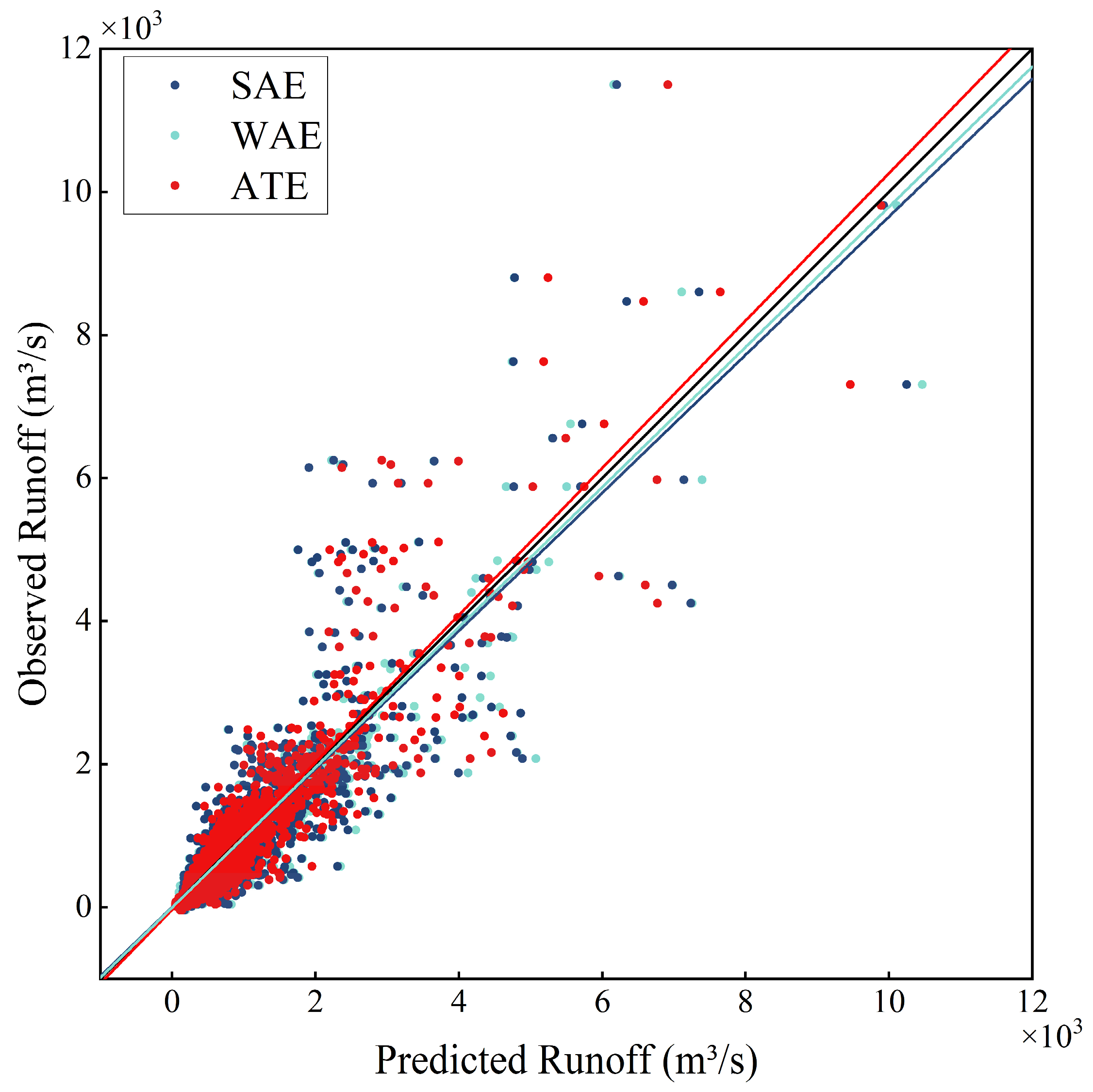
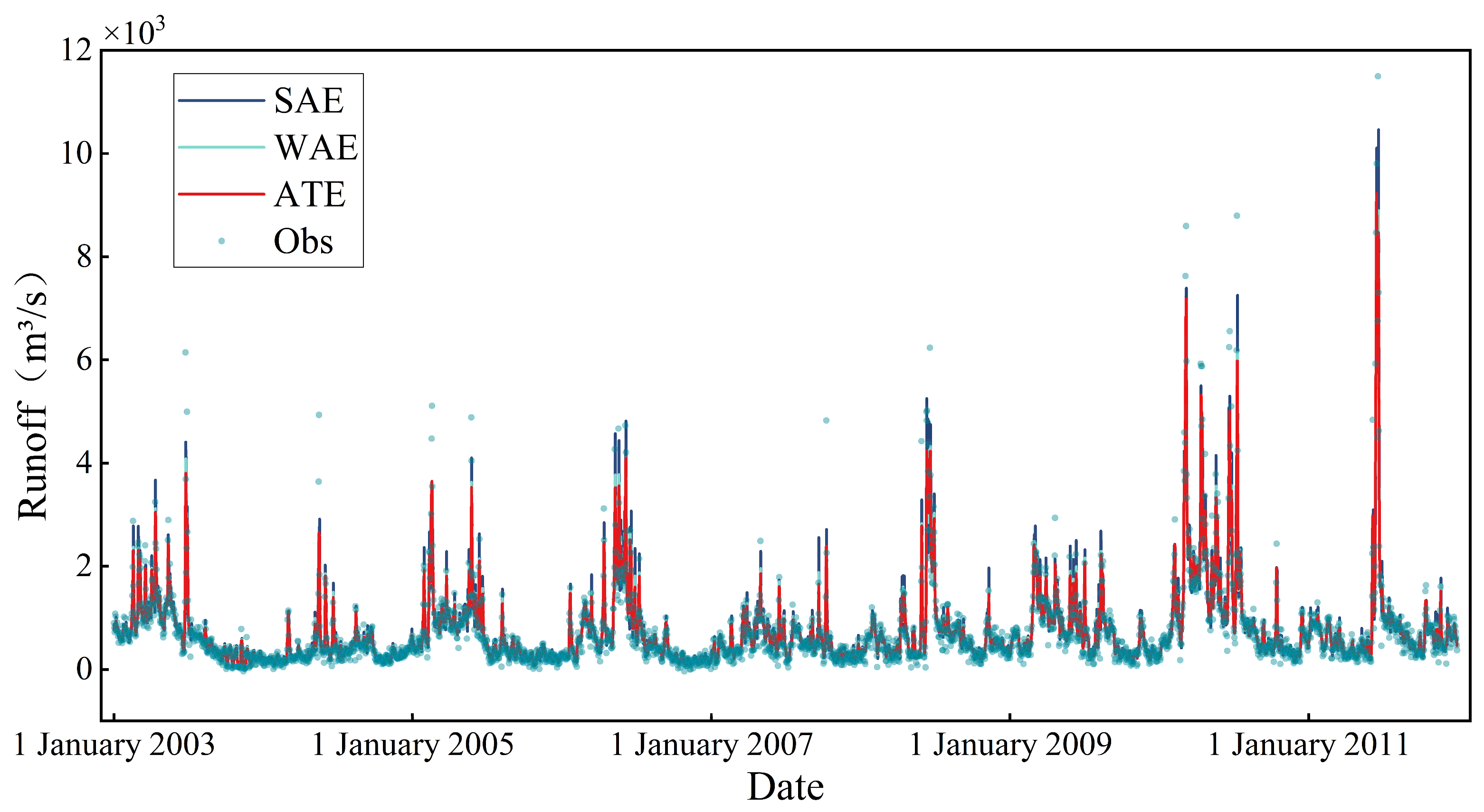
4.3. Comparison of Ensemble Models

Figure 8 shows predicted and observed daily runoff scatter plots of three stacking models, including SAE, WAE, and ATE. As shown in the figure, the fitting line of the ATE model displays the smallest deviation when compared to the other stacking models. From the detailed comparison of the different stacking models with ATE, it can be seen that the four evaluation criteria of the ATE models were superior to those of the SAE and WAE models. Compared with the SAE and WAE models, the ATE model has a 10.32% and 8.54% increase in NSE, an 18.65% and 16.38% reduction in RMSE, a 25.93% and 18.66% reduction in MAE, and a 4.97% and 4.19% increase in r. This outcome serves as evidence for the effectiveness of the proposed ensemble model.
The differences in predicted runoff amongst the various stacking models are shown in Figure 9. As can be seen in Figure 9, the predicted values of the ATE model approximated the observed values better than the SAE and WAE models, and the scatter points in Figure 8 were more closely distributed around the regression line. Thus, it demonstrates the superiority of the proposed stacking model based on the attention mechanism compared to other models. Moreover, all of the models exhibited a tendency to underestimate runoff during high runoff periods. Nonetheless, the ATE model demonstrated a smaller prediction error compared to the other models. In summary, this finding further confirms the superiority of ATE over the comparative models.

4.4. Comparison of Model Performance in Significance Tests

In this study, 10-fold cross-validation was performed to obtain the ranking of six ensemble models on different validation sets. The average ranking of each model under different evaluation criteria is shown in Table 4. The p-values of the Friedman tests for NSE, RMSE, MAE, and r are 1.03 × 10⁻⁵, 5.64 × 10⁻⁴, 2.54 × 10⁻⁵, and 6.92 × 10⁻⁷, respectively, and they are all less than 0.001, indicating that the six ensemble models considered for comparison are significantly different at the α = 0.1% significance level. In terms of NSE, RMSE, and r, the average ranking of evaluation criteria was consistent across all models, from best to worst for ATE, WAE, XGB, SAE, RF, and AdaBoost, respectively. It means that the ATE and AdaBoost models are the best and the worst of the six models, respectively. In terms of MAE, the two best performing models are ATE and WAE, but the worst model is XGB, which outperforms in the other three metrics.
As significant differences were found among the six models, this study used a post hoc test (Nemenyi test) to check whether the ATE model (the best model) is significantly better than the other models. When the number of comparison models was 6 and the dataset was 10, the CD at 5% and 10% significance levels were calculated to be 2.38 and 2.17, respectively. The average ranking of each model in Table 4 was subtracted from the ranking of the ATE model separately to obtain the respective ARD (Table 5). At the 5% level of significance, the ATE model was significantly different from that of RF, AdaBoost, and SAE in terms of NSE, RMSE, and r, and significantly outperformed RF, XGB, and SAE in terms of MAE. At the 10% level of significance, the ATE model was significantly different from all other models except the WAE model.

5. Discussion

The proposed stacking ensemble model for reservoir inflow is promising as it offers improvements over each of the base models. However, it is worth exploring how the attention ensemble model combines the base models. To obtain a more intuitive understanding of the mechanism of the attention ensemble model, the study summed the weights of the three base models in the stacking ensemble models to obtain the attention level of each ensemble model to each base model. Figure 10 shows the visualization results for the weights of the ensemble model. As shown in the figure, the weights of the base models of the ATE model are more concentrated whereas those for the WAE model are more discrete. In the WAE model, since the base models’ weights are determined based on the square of the deviation, the AdaBoost model, which had a smaller MAE score, obtains a higher weight. The performance of the base models has a negative correlation with the weights of the base models in the ATE model. The highest weights are assigned to XGB, which has the best performance in the base model. In addition, the attention mechanism also gives a certain weight to the poorly performing models compared to the normal stacking ensemble model, which can better utilize the variability between the base models to correct the prediction errors to generate more accurate predictions.
This study demonstrates that improvements in prediction performance can be obtained by combining various machine learning models. It is worth noting that even the simplest ensemble model can bring an improvement to the prediction results of machine learning models. Thus, the simple averaging method is effective and hard-to-beat in practice [54,55]. Tyralis et al. [56] proposed stacking of quantile regression and quantile regression forests to postprocess hydrological model simulations, and the ensemble model outperforms simple averaging with the maximum obtained improvement approximately equal to 2%. Granata et al. [57] proposed a stacking model based on elastic networks and found that the model outperformed the bidirectional LSTM network model for peak flow prediction in several cases. The attention ensemble model proposed in this study obtained a maximum improvement of about 5% compared to simple averaging, confirming the validity of the proposed model. The advantage of the ATE model is that it can adaptively learn the weights of each base model to better take advantage of the base models. Specifically, the attention mechanism can adaptively adjust the contribution of each base model according to the situation of different data points, so that the performance of each base model can be better utilized at different data points. In contrast, other meta models may require manually specifying the weights of each base model or using a simple average or weighted average to combine the predictions of the base models. These approaches may not take full advantage of the characteristics and strengths of each base model, resulting in a limited improvement in overall performance. Gu et al. [58] applied the stacking model based on multiple linear regression to rainfall prediction and found that the ANN model generally outperformed the stacking model, mainly because most machine learning models underestimated the extreme precipitation, while the proposed stacking model in the study by Gu et al. [58] did not give sufficient weight to the base model with good simulation results at extreme points. Owing to the attention mechanism, the ATE model tends to give more weight to the base model based on the model’s superior performance compared to other common stacked models. Therefore, it performs better than other stacked models in extreme value simulations. In addition, unlike the super ensemble learning proposed by Tyralis [59], the ATE model can weight the output of the base models to highlight the important features. This can avoid the influence of excessive noise and irrelevant features on the meta model, thus improving the stability and accuracy of the model.
According to the results of the average ranking of the evaluation criteria, the ATE model outperformed the WAE model, but the ATE model is not statistically significantly different from the WAE model. It is possibly due to the fact that only 10-fold cross-validation was selected in this study, and it is insufficient to reach a larger CD value. The advantages of the ATE model over the traditional stacked model may be more evident if the dataset used for significance testing is large enough.
However, it has been suggested that, as the number of base models increases, weight optimization may not have a significant improvement relative to simple averaging [59]. A large number of base models could result in overfitting that leads to degraded stacking model performance [60]. Therefore, although the current research progress shows that there is a general trend toward constructing ensemble forecasting, it is still important to improve model accuracy through preprocessing and model evaluation improvements [61,62].

6. Conclusions

This study introduces a novel stacking ensemble model based on the attention mechanism to enhance the performance of machine learning models in the prediction of reservoir inflow, utilizing data from the Fuchun River basin in China. This study used three typical ensemble machine learning models (RF, AdaBoost, and XGB) for prediction. The results showed that the three machine learning models performed well enough to meet the requirements as base models in the stacking ensemble model and the XGB model outperformed the other two models. To improve the generalizability and the performance of the machine learning models, the study combined the outputs of the three models as inputs to the proposed model. To verify the superiority of the proposed model, this study used four evaluation criteria and two comparison models (SAE and WAT) to test model performance. Compared with base models, the stacking ensemble models generally achieved better prediction results. In addition, comparing the proposed model with the common stacking ensemble models shows that the proposed model has significant superiority and enhances the generalization ability of the machine learning model. Therefore, the proposed stacking ensemble model can generate rational and precise forecasts for the reservoir inflow.
Despite its promising performance, the proposed model has certain limitations that must be acknowledged. Specifically, the study highlights the susceptibility of the model’s superior predictive performance to disruption by models with inferior performance during the daily runoff forecast ensemble process. As a result, there is a pressing need to devise more effective methods of ensembling these models. Additionally, although the deep learning ensemble models show promise, further research into more advanced ensemble methods is warranted.

Author Contributions

Conceptualization, M.L. and L.C.; methodology, M.L., Q.H., S.Q. and L.C.; validation, M.L., S.Q. and L.Z.; formal analysis, M.L., Q.H., D.H. and X.W.; data curation, M.L. and Q.H.; writing—original draft preparation, M.L.; writing—review and editing, M.L., Q.H., S.Q., L.Z., D.H., X.W. and L.C.; funding acquisition, L.C. All authors have read and agreed to the published version of the manuscript.

Funding

This research was funded by the National Key Research and Development Program of China (2022YFC3202804), the National Natural Science Foundation of China (41890822), and the Natural Science Foundation of Hubei Province of China (2022CFA094).

Data Availability Statement

Not applicable.

Acknowledgments

The authors appreciate the reviewers and editors for their constructive comments that greatly helped to improve the study.

Conflicts of Interest

The authors declare no conflict of interest.

References

  1. Kratzert, F.; Klotz, D.; Herrnegger, M.; Sampson, A.K.; Hochreiter, S.; Nearing, G.S. Toward Improved Predictions in Ungauged Basins: Exploiting the Power of Machine Learning. Water Resour. Res. 2019, 55, 11344–11354. [Google Scholar] [CrossRef] [Green Version]
  2. Alfieri, L.; Burek, P.; Dutra, E.; Krzeminski, B.; Muraro, D.; Thielen, J.; Pappenberger, F. GloFAS—Global Ensemble Streamflow Forecasting and Flood Early Warning. Hydrol. Earth Syst. Sci. 2013, 17, 1161–1175. [Google Scholar] [CrossRef] [Green Version]
  3. Qin, P.; Xu, H.; Liu, M.; Du, L.; Xiao, C.; Liu, L.; Tarroja, B. Climate Change Impacts on Three Gorges Reservoir Impoundment and Hydropower Generation. J. Hydrol. 2020, 580, 123922. [Google Scholar] [CrossRef]
  4. Zhang, Y.; Cheng, L.; Zhang, L.; Qin, S.; Liu, L.; Liu, P.; Liu, Y. Does Non-Stationarity Induced by Multiyear Drought Invalidate the Paired-Catchment Method? Hydrol. Earth Syst. Sci. 2022, 26, 6379–6397. [Google Scholar] [CrossRef]
  5. IPCC. Global Warming of 1.5 °C: IPCC Special Report on Impacts of Global Warming of 1.5 °C above Pre-Industrial Levels in Context of Strengthening Response to Climate Change, Sustainable Development, and Efforts to Eradicate Poverty, 1st ed.; Cambridge University Press: Cambridge, UK, 2022; ISBN 978-1-00-915794-0. [Google Scholar]
  6. Zhang, R.; Cheng, L.; Liu, P.; Huang, K.; Gong, Y.; Qin, S.; Liu, D. Effect of GCM Credibility on Water Resource System Robustness under Climate Change Based on Decision Scaling. Adv. Water Resour. 2021, 158, 104063. [Google Scholar] [CrossRef]
  7. Wang, W.-C.; Chau, K.-W.; Cheng, C.-T.; Qiu, L. A Comparison of Performance of Several Artificial Intelligence Methods for Forecasting Monthly Discharge Time Series. J. Hydrol. 2009, 374, 294–306. [Google Scholar] [CrossRef] [Green Version]
  8. Yuan, X.; Chen, C.; Lei, X.; Yuan, Y.; Muhammad Adnan, R. Monthly Runoff Forecasting Based on LSTM–ALO Model. Stoch Env. Res Risk Assess 2018, 32, 2199–2212. [Google Scholar] [CrossRef]
  9. Yang, T.; Asanjan, A.A.; Welles, E.; Gao, X.; Sorooshian, S.; Liu, X. Developing Reservoir Monthly Inflow Forecasts Using Artificial Intelligence and Climate Phenomenon Information. Water Resour. Res. 2017, 53, 2786–2812. [Google Scholar] [CrossRef]
  10. Vázquez, R.F.; Feyen, J. Assessment of the Effects of DEM Gridding on the Predictions of Basin Runoff Using MIKE SHE and a Modelling Resolution of 600m. J. Hydrol. 2007, 334, 73–87. [Google Scholar] [CrossRef]
  11. Fang, Y.-H.; Zhang, X.; Corbari, C.; Mancini, M.; Niu, G.-Y.; Zeng, W. Improving the Xin’anjiang Hydrological Model Based on Mass–Energy Balance. Hydrol. Earth Syst. Sci. 2017, 21, 3359–3375. [Google Scholar] [CrossRef] [Green Version]
  12. Su, H.; Cheng, L.; Wu, Y.; Qin, S.; Liu, P.; Zhang, Q.; Cheng, S.; Li, Y. Extreme Storm Events Shift DOC Export from Transport-Limited to Source-Limited in a Typical Flash Flood Catchment. J. Hydrol. 2023, 620, 129377. [Google Scholar] [CrossRef]
  13. Wu, M.-C.; Lin, G.-F. The Very Short-Term Rainfall Forecasting for a Mountainous Watershed by Means of an Ensemble Numerical Weather Prediction System in Taiwan. J. Hydrol. 2017, 546, 60–70. [Google Scholar] [CrossRef]
  14. Mignot, E.; Li, X.; Dewals, B. Experimental Modelling of Urban Flooding: A Review. J. Hydrol. 2019, 568, 334–342. [Google Scholar] [CrossRef] [Green Version]
  15. Salas, J.D.; Tabios, G.Q.; Bartolini, P. Approaches to Multivariate Modeling of Water Resources Time Series. J. Am. Water Resour. Assoc. 1985, 21, 683–708. [Google Scholar] [CrossRef]
  16. Montanari, A.; Rosso, R.; Taqqu, M.S. Fractionally Differenced ARIMA Models Applied to Hydrologic Time Series: Identification, Estimation, and Simulation. Water Resour. Res. 1997, 33, 1035–1044. [Google Scholar] [CrossRef]
  17. Cheng, S.; Cheng, L.; Qin, S.; Zhang, L.; Liu, P.; Liu, L.; Xu, Z.; Wang, Q. Improved Understanding of How Catchment Properties Control Hydrological Partitioning Through Machine Learning. Water Resour. Res. 2022, 58, e2021WR031412. [Google Scholar] [CrossRef]
  18. Yaseen, Z.M.; Jaafar, O.; Deo, R.C.; Kisi, O.; Adamowski, J.; Quilty, J.; El-Shafie, A. Stream-Flow Forecasting Using Extreme Learning Machines: A Case Study in a Semi-Arid Region in Iraq. J. Hydrol. 2016, 542, 603–614. [Google Scholar] [CrossRef]
  19. Bray, M.; Han, D. Identification of Support Vector Machines for Runoff Modelling. J. Hydroinformatics 2004, 6, 265–280. [Google Scholar] [CrossRef] [Green Version]
  20. Hochreiter, S.; Schmidhuber, J. Long Short-Term Memory. Neural Comput. 1997, 9, 1735–1780. [Google Scholar] [CrossRef]
  21. Chang, F.-J.; Chen, P.-A.; Lu, Y.-R.; Huang, E.; Chang, K.-Y. Real-Time Multi-Step-Ahead Water Level Forecasting by Recurrent Neural Networks for Urban Flood Control. J. Hydrol. 2014, 517, 836–846. [Google Scholar] [CrossRef]
  22. Carlson, R.F.; MacCormick, A.J.A.; Watts, D.G. Application of Linear Random Models to Four Annual Streamflow Series. Water Resour. Res. 1970, 6, 1070–1078. [Google Scholar] [CrossRef]
  23. Burlando, P.; Rosso, R.; Cadavid, L.G.; Salas, J.D. Forecasting of Short-Term Rainfall Using ARMA Models. J. Hydrol. 1993, 144, 193–211. [Google Scholar] [CrossRef]
  24. Rahman, M.A.; Yunsheng, L.; Sultana, N. Analysis and Prediction of Rainfall Trends over Bangladesh Using Mann–Kendall, Spearman’s Rho Tests and ARIMA Model. Meteorol. Atmos. Phys. 2017, 129, 409–424. [Google Scholar] [CrossRef]
  25. Liu, S.; Xu, J.; Zhao, J.; Xie, X.; Zhang, W. Efficiency Enhancement of a Process-Based Rainfall–Runoff Model Using a New Modified AdaBoost.RT Technique. Appl. Soft Comput. 2014, 23, 521–529. [Google Scholar] [CrossRef]
  26. Xie, T.; Zhang, G.; Hou, J.; Xie, J.; Lv, M.; Liu, F. Hybrid Forecasting Model for Non-Stationary Daily Runoff Series: A Case Study in the Han River Basin, China. J. Hydrol. 2019, 577, 123915. [Google Scholar] [CrossRef]
  27. Xiang, Z.; Yan, J.; Demir, I. A Rainfall-Runoff Model With LSTM-Based Sequence-to-Sequence Learning. Water Resour. Res. 2020, 56, e2019WR025326. [Google Scholar] [CrossRef]
  28. Chen, X.; Huang, J.; Han, Z.; Gao, H.; Liu, M.; Li, Z.; Liu, X.; Li, Q.; Qi, H.; Huang, Y. The Importance of Short Lag-Time in the Runoff Forecasting Model Based on Long Short-Term Memory. J. Hydrol. 2020, 589, 125359. [Google Scholar] [CrossRef]
  29. Renard, B.; Kavetski, D.; Kuczera, G.; Thyer, M.; Franks, S.W. Understanding Predictive Uncertainty in Hydrologic Modeling: The Challenge of Identifying Input and Structural Errors: Identifiability of Input and Structural Errors. Water Resour. Res. 2010, 46, W05521. [Google Scholar] [CrossRef]
  30. Liu, G.; Tang, Z.; Qin, H.; Liu, S.; Shen, Q.; Qu, Y.; Zhou, J. Short-Term Runoff Prediction Using Deep Learning Multi-Dimensional Ensemble Method. J. Hydrol. 2022, 609, 127762. [Google Scholar] [CrossRef]
  31. Baran, S.; Hemri, S.; El Ayari, M. Statistical Postprocessing of Water Level Forecasts Using Bayesian Model Averaging with Doubly Truncated Normal Components. Water Resour. Res. 2019, 55, 3997–4013. [Google Scholar] [CrossRef] [Green Version]
  32. Jiang, S.; Ren, L.; Xu, C.-Y.; Liu, S.; Yuan, F.; Yang, X. Quantifying Multi-Source Uncertainties in Multi-Model Predictions Using the Bayesian Model Averaging Scheme. Hydrol. Res. 2018, 49, 954–970. [Google Scholar] [CrossRef]
  33. Höge, M.; Guthke, A.; Nowak, W. The Hydrologist’s Guide to Bayesian Model Selection, Averaging and Combination. J. Hydrol. 2019, 572, 96–107. [Google Scholar] [CrossRef]
  34. Diks, C.G.H.; Vrugt, J.A. Comparison of Point Forecast Accuracy of Model Averaging Methods in Hydrologic Applications. Stoch Environ. Res. Risk. Assess 2010, 24, 809–820. [Google Scholar] [CrossRef] [Green Version]
  35. Sun, W.; Trevor, B. A Stacking Ensemble Learning Framework for Annual River Ice Breakup Dates. J. Hydrol. 2018, 561, 636–650. [Google Scholar] [CrossRef]
  36. Ho, T.K. Random Decision Forests. In Proceedings of the Third International Conference on Document Analysis and Recognition, Montreal, QC, Canada, 14–16 August 1995; IEEE Computer Society: Washington, DC, USA, 1995; Volume 1, p. 278. [Google Scholar]
  37. Breiman, L. Random Forests. Mach. Learn. 2001, 45, 5–32. [Google Scholar] [CrossRef] [Green Version]
  38. Loken, E.D.; Clark, A.J.; McGovern, A.; Flora, M.; Knopfmeier, K. Postprocessing Next-Day Ensemble Probabilistic Precipitation Forecasts Using Random Forests. Weather Forecast. 2019, 34, 2017–2044. [Google Scholar] [CrossRef]
  39. Yang, J.; Huang, X. The 30 m Annual Land Cover Dataset and Its Dynamics in China from 1990 to 2019. Earth Syst. Sci. Data 2021, 13, 3907–3925. [Google Scholar] [CrossRef]
  40. Towfiqul Islam, A.R.M.; Talukdar, S.; Mahato, S.; Kundu, S.; Eibek, K.U.; Pham, Q.B.; Kuriqi, A.; Linh, N.T.T. Flood Susceptibility Modelling Using Advanced Ensemble Machine Learning Models. Geosci. Front. 2021, 12, 101075. [Google Scholar] [CrossRef]
  41. Srivastava, R.; Tiwari, A.N.; Giri, V.K. Solar Radiation Forecasting Using MARS, CART, M5, and Random Forest Model: A Case Study for India. Heliyon 2019, 5, e02692. [Google Scholar] [CrossRef] [Green Version]
  42. Zhang, W.; Wu, C.; Zhong, H.; Li, Y.; Wang, L. Prediction of Undrained Shear Strength Using Extreme Gradient Boosting and Random Forest Based on Bayesian Optimization. Geosci. Front. 2021, 12, 469–477. [Google Scholar] [CrossRef]
  43. Freund, Y.; Schapire, R. Experiments with a New Boosting Algorithm. In Proceedings of the Thirteenth International Conference on International Conference on Machine Learning, Bari, Italy, 3–6 July 1996; Morgan Kaufmann Publishers Inc.: San Francisco, CA, USA, 1996; pp. 148–156. [Google Scholar]
  44. Friedman, J.; Hastie, T.; Tibshirani, R. Additive Logistic Regression: A Statistical View of Boosting (With Discussion and a Rejoinder by the Authors). Ann. Statist. 2000, 28, 337–407. [Google Scholar] [CrossRef]
  45. Chen, T.; Guestrin, C. XGBoost: A Scalable Tree Boosting System. In Proceedings of the 22nd ACM SIGKDD International Conference on Knowledge Discovery and Data Mining, San Francisco, CA, USA, 13 August 2016; ACM: New York, NY, USA; pp. 785–794. [Google Scholar]
  46. Fan, J.; Yue, W.; Wu, L.; Zhang, F.; Cai, H.; Wang, X.; Lu, X.; Xiang, Y. Evaluation of SVM, ELM and Four Tree-Based Ensemble Models for Predicting Daily Reference Evapotranspiration Using Limited Meteorological Data in Different Climates of China. Agric. For. Meteorol. 2018, 263, 225–241. [Google Scholar] [CrossRef]
  47. Jia, Y.; Jin, S.; Savi, P.; Gao, Y.; Tang, J.; Chen, Y.; Li, W. GNSS-R Soil Moisture Retrieval Based on a XGboost Machine Learning Aided Method: Performance and Validation. Remote Sens. 2019, 11, 1655. [Google Scholar] [CrossRef] [Green Version]
  48. Tahmassebi, A.; Wengert, G.J.; Helbich, T.H.; Bago-Horvath, Z.; Alaei, S.; Bartsch, R.; Dubsky, P.; Baltzer, P.; Clauser, P.; Kapetas, P.; et al. Impact of Machine Learning with Multiparametric Magnetic Resonance Imaging of the Breast for Early Prediction of Response to Neoadjuvant Chemotherapy and Survival Outcomes in Breast Cancer Patients. Investig. Radiol. 2019, 54, 110–117. [Google Scholar] [CrossRef]
  49. Wolpert, D.H. Stacked Generalization. Neural Netw. 1992, 5, 241–259. [Google Scholar] [CrossRef]
  50. Zhou, Z.-H. Ensemble Learning. In Encyclopedia of Biometrics; Li, S.Z., Jain, A.K., Eds.; Springer US: Boston, MA, USA, 2015; pp. 411–416. ISBN 978-1-4899-7487-7. [Google Scholar]
  51. Ghahramani, Z. Probabilistic Machine Learning and Artificial Intelligence. Nature 2015, 521, 452–459. [Google Scholar] [CrossRef]
  52. Shang, Q.; Lin, C.; Yang, Z.; Bing, Q.; Zhou, X. A Hybrid Short-Term Traffic Flow Prediction Model Based on Singular Spectrum Analysis and Kernel Extreme Learning Machine. PLoS ONE 2016, 11, e0161259. [Google Scholar] [CrossRef] [Green Version]
  53. Zhang, X.; Xu, Y.-P.; Fu, G. Uncertainties in SWAT Extreme Flow Simulation under Climate Change. J. Hydrol. 2014, 515, 205–222. [Google Scholar] [CrossRef]
  54. Lichtendahl, K.C.; Grushka-Cockayne, Y.; Winkler, R.L. Is It Better to Average Probabilities or Quantiles? Manag. Sci. 2013, 59, 1594–1611. [Google Scholar] [CrossRef]
  55. Stock, J.H.; Watson, M.W. Combination Forecasts of Output Growth in a Seven-Country Data Set. J. Forecast. 2004, 23, 405–430. [Google Scholar] [CrossRef]
  56. Tyralis, H.; Papacharalampous, G.; Burnetas, A.; Langousis, A. Hydrological Post-Processing Using Stacked Generalization of Quantile Regression Algorithms: Large-Scale Application over CONUS. J. Hydrol. 2019, 577, 123957. [Google Scholar] [CrossRef]
  57. Granata, F.; Di Nunno, F.; de Marinis, G. Stacked Machine Learning Algorithms and Bidirectional Long Short-Term Memory Networks for Multi-Step Ahead Streamflow Forecasting: A Comparative Study. J. Hydrol. 2022, 613, 128431. [Google Scholar] [CrossRef]
  58. Gu, J.; Liu, S.; Zhou, Z.; Chalov, S.R.; Zhuang, Q. A Stacking Ensemble Learning Model for Monthly Rainfall Prediction in the Taihu Basin, China. Water 2022, 14, 492. [Google Scholar] [CrossRef]
  59. Tyralis, H.; Papacharalampous, G.; Langousis, A. Super Ensemble Learning for Daily Streamflow Forecasting: Large-Scale Demonstration and Comparison with Multiple Machine Learning Algorithms. Neural. Comput. Applic. 2021, 33, 3053–3068. [Google Scholar] [CrossRef]
  60. Kim, D.; Yu, H.; Lee, H.; Beighley, E.; Durand, M.; Alsdorf, D.E.; Hwang, E. Ensemble Learning Regression for Estimating River Discharges Using Satellite Altimetry Data: Central Congo River as a Test-Bed. Remote Sens. Environ. 2019, 221, 741–755. [Google Scholar] [CrossRef]
  61. Slater, L.J.; Villarini, G. Enhancing the Predictability of Seasonal Streamflow with a Statistical-Dynamical Approach. Geophys. Res. Lett. 2018, 45, 6504–6513. [Google Scholar] [CrossRef]
  62. Gibbs, M.S.; McInerney, D.; Humphrey, G.; Thyer, M.A.; Maier, H.R.; Dandy, G.C.; Kavetski, D. State Updating and Calibration Period Selection to Improve Dynamic Monthly Streamflow Forecasts for an Environmental Flow Management Application. Hydrol. Earth Syst. Sci. 2018, 22, 871–887. [Google Scholar] [CrossRef] [Green Version]
Figure 1. Diagram of the k-fold cross validation.
Water 15 01265 g001
Figure 2. Flow chart for the construction of the proposed attention ensemble model in this study.
Water 15 01265 g002
Figure 3. Location of the Qiantang River basin.
Water 15 01265 g003
Figure 4. Precipitation and runoff distribution in the Qiantang River basin from 1970 to 2011.
Water 15 01265 g004
Figure 5. Training set and testing set division scheme.
Water 15 01265 g005
Figure 6. Box plots showing the evaluation criteria in different models. Each box is calculated from 10 folds of the training data model runs. The model performances vary in terms of (a) NSE, (b) RMSE, (c) MAE, and (d) r. The × marks inside the boxes are the average values.
Water 15 01265 g006
Figure 7. Runoff predicted by three base models against observations during the testing period: (a) RF, (b) AdaBoost, and (c) XGB.
Water 15 01265 g007
Figure 8. Scatter plot displaying the correlation between the predicted and observed runoff of the stacking models.
Water 15 01265 g008
Figure 9. Prediction results of the stacking models in the testing period.
Water 15 01265 g009
Figure 10. Visualization results for base model weights. The solid lines inside the boxes are the average values.
Water 15 01265 g010
Table 1. Summary of the hyper-parameters for the three machine learning models.
ModelModel Hyper-Parameters
Random Forest (RF)n_estimators = 600
criterion = squared_error
max_depth = None
min_samples_split = 2
min_samples_leaf = 1
Adaptive Boosting (AdaBoost)n_estimators = 30
learning_rate = 0.08
base_estimator = DecisionTreeRegressor
max_depth = None
min_samples_split = 26
min_samples_leaf = 9
Extreme Gradient Boosting (XGB)n_estimators = 200
learning_rate = 0.02
subsample = 0.22
colsample_bytree = 0.96
Table 2. Evaluation criteria for three base models (the values of RMSE and MAE are in m3/s).
PeriodModelsNSERMSEMAEr
ValidationRF0.690 (0.063)559.8 (111.3)267.6 (43.3)0.836 (0.030)
AdaBoost0.685 (0.066)564.2 (118.2)263.4 (45.7)0.834 (0.032)
XGB0.704 (0.057)550.0 (121.9)265.3 (43.3)0.843 (0.031)
TestingRF0.757 (0.007)416.3 (6.4)204.4 (2.3)0.870 (0.003)
AdaBoost0.762 (0.014)411.7 (12.1)197.3 (2.4)0.872 (0.007)
XGB0.767 (0.005)407.4 (4.0)205.5 (2.2)0.880 (0.003)
Note: The values in the table are means of 10 folds, with standard deviations in parentheses.
Table 3. Evaluation criteria of three stacking models (the values of RMSE and MAE are in m3/s).
ModelsNSERMSEMAEr
SAE0.766408.0199.30.876
WAE0.779397.0181.50.883
ATE0.845331.9147.60.920
Table 4. The average ranking of each model in each fold for NSE, RMSE, MAE, and r.
ModelsRanking (NSE)Ranking (RMSE)Ranking (MAE)Ranking (r)
RF4.84.44.75.0
AdaBoost5.24.73.45.3
XGB3.33.85.13.3
SAE3.74.03.83.9
WAE2.92.72.82.4
ATE1.11.41.21.1
τχ230.8021.8328.8036.69
p1.03 × 10−55.64 × 10−42.54 × 10−56.92 × 10⁻⁷
Table 5. The ARD of each model in each fold for NSE, RMSE, MAE, and r.
ModelsARD (NSE)ARD (RMSE)ARD (MAE)ARD (r)
RF3.73.03.53.9
AdaBoost4.13.32.24.2
XGB2.22.43.92.2
SAE2.62.62.62.8
WAE1.81.31.61.3
Disclaimer/Publisher’s Note: The statements, opinions and data contained in all publications are solely those of the individual author(s) and contributor(s) and not of MDPI and/or the editor(s). MDPI and/or the editor(s) disclaim responsibility for any injury to people or property resulting from any ideas, methods, instructions or products referred to in the content.

