Flood Frequency Analysis Using the Gamma Family Probability Distributions


Abstract
:1. Introduction
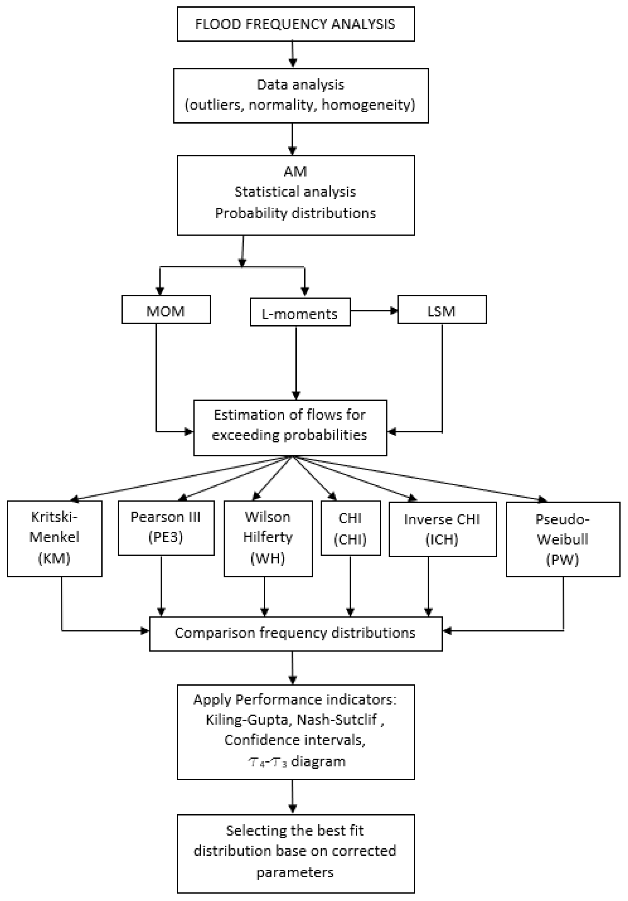
2. Methodology

| Statistical Parameters | Quantitative Measures | |
|---|---|---|
| MOM | L-Moments | |
| Expected value (arithmetic mean) | ||
| Coefficient of variation/L-coefficient of variation | ||
| Skewness/L-skewness | ||
| Skewness chosen in Romania | ||
2.1. Probability Distributions
2.2. Kritsky–Menkel (KM)
2.3. Pearson III (PE3)
2.4. Wilson–Hilferty (WH)
2.5. Chi Distribution (CHI)
2.6. Inverse Chi Distribution (ICH)
2.7. Pseudo-Weibull Distribution (PW)
3. Parameter Estimation
3.1. Kritsky–Menkel
3.2. Pearson III
3.3. Wilson–Hilferty
3.4. Chi Distribution
3.5. Inverse Chi Distribution
3.6. Pseudo-Weibull Distribution
4. The Choice of Skewness
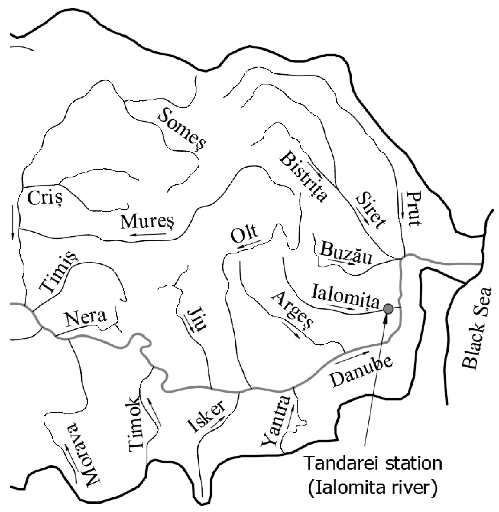
5. Application to Hydrologic Data
| (m3/s) | (m3/s) | (-) | (-) | (-) | (m3/s) | (m3/s) | (m3/s) | (m3/s) | (-) | (-) | (-) |
|---|---|---|---|---|---|---|---|---|---|---|---|
| 224.1 | 118 | 0.527 | 0.327 | 2.074 | 224.1 | 68.6 | 6.13 | 1.69 | 0.306 | 0.089 | 0.025 |
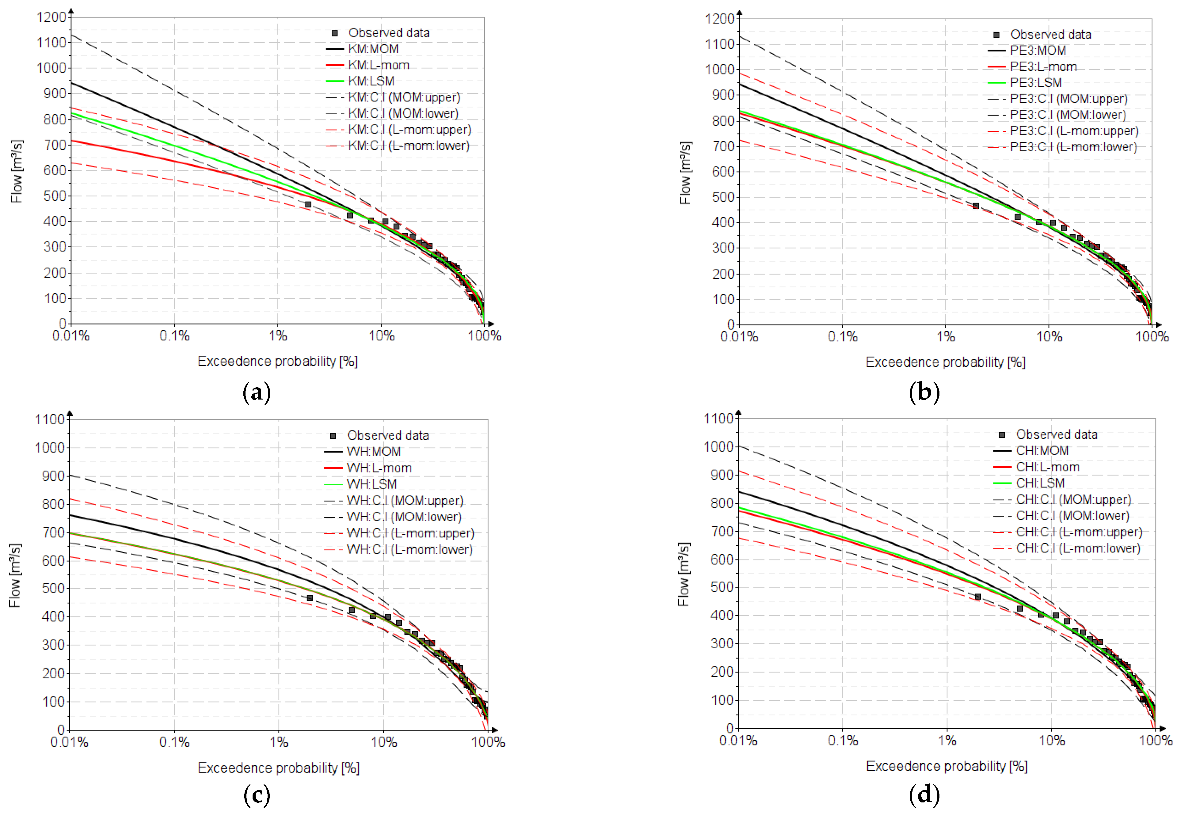
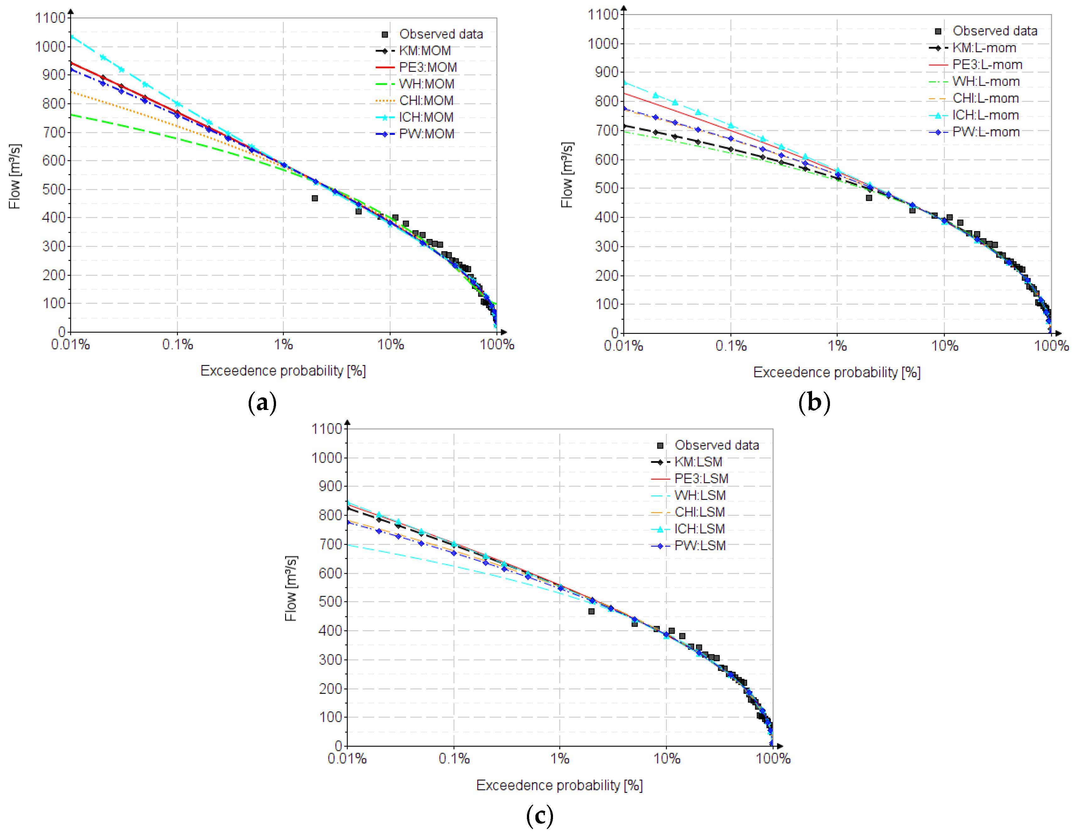
6. Results
- -
- Nash–Sutcliffe coefficient (E):
- -
- Kling–Gupta coefficient (KGE):
7. Discussion
8. Conclusions
Supplementary Materials
Author Contributions
Funding
Institutional Review Board Statement
Informed Consent Statement
Data Availability Statement
Conflicts of Interest
Abbreviations
| MOM | the method of ordinary moments |
| L-moments | the method of linear moments |
| LSM | the method of least squares |
| expected value; arithmetic mean | |
| standard deviation | |
| coefficient of variation | |
| coefficient of skewness; skewness | |
| linear moments | |
| coefficient of variation based on the L-moments method | |
| coefficient of skewness based on the L-moments method | |
| coefficient of kurtosis based on the L-moments method | |
| multiplication factor | |
| PE3 | Pearson III distribution |
| KM | Kristky–Menkel distribution |
| WH | Wilson–Hilferty distribution |
| CHI | three-parameter chi distribution |
| ICH | three-parameter inverse chi distribution |
| PW | pseudo-Weibull distribution |
| INHGA | The National Institute of Hydrology and Water Management |
Appendix A. The Variation of L-Skewness and L-Kurtosis
Appendix B. The Frequency Factors for the Analyzed Distributions
| Distribution | ||
|---|---|---|
| Quantile Function (Inverse Function) | ||
| Method of Ordinary Moments (MOM) | L-Moments | |
| KM | ||
| PE3 | ||
| WH | ||
| CHI | ||
| ICH | ||
| PW | ||
Appendix C. Estimation of the Frequency Factor for the PE3 Distribution
| P (%) | a | b | c | d | e | f | g | h |
|---|---|---|---|---|---|---|---|---|
| 0.01 | 3.71828 | 2.146200 | 1.55790 × 10⁻¹ | −7.69315 × 10⁻² | 1.50378 × 10⁻² | −1.72710 × 10⁻³ | 1.1060 × 10⁻⁴ | −3.033 × 10⁻⁶ |
| 0.1 | 3.09014 | 1.426290 | 4.96310 × 10⁻² | −4.21189 × 10⁻² | 7.94983 × 10⁻³ | −8.33091 × 10⁻⁴ | 4.7935 × 10⁻⁵ | −1.179 × 10⁻⁶ |
| 0.5 | 2.57601 | 0.937811 | −4.85114 × 10⁻³ | −2.43670 × 10⁻² | 4.59158 × 10⁻³ | −4.29197 × 10⁻⁴ | 2.0466 × 10⁻⁵ | −3.82 × 10⁻⁷ |
| 1 | 2.32661 | 0.733146 | −2.18707 × 10⁻² | −1.85502 × 10⁻² | 3.58677 × 10⁻³ | −3.15387 × 10⁻⁴ | 1.3017 × 10⁻⁵ | −1.71 × 10⁻⁷ |
| 2 | 2.05408 | 0.533496 | −3.42010 × 10⁻² | −1.38703 × 10⁻² | 2.86305 × 10⁻³ | −2.39574 × 10⁻⁴ | 8.3060 × 10⁻⁶ | −4.17 × 10⁻⁸ |
| 3 | 1.88115 | 0.419782 | −3.89303 × 10⁻² | −1.16643 × 10⁻² | 2.57668 × 10⁻³ | −2.13746 × 10⁻⁴ | 6.8730 × 10⁻⁶ | −5.63 × 10⁻⁹ |
| 5 | 1.64524 | 0.280836 | −4.18754 × 10⁻² | −9.45489 × 10⁻³ | 2.37315 × 10⁻³ | −2.02670 × 10⁻⁴ | 6.5730 × 10⁻⁶ | −4.92 × 10⁻⁹ |
| 10 | 1.28196 | 0.103328 | −3.95043 × 10⁻² | −7.48248 × 10⁻³ | 2.41382 × 10⁻³ | −2.31322 × 10⁻⁴ | 8.9870 × 10⁻⁶ | −8.238 × 10⁻⁸ |
| 20 | 0.842052 | −0.0526706 | −2.7535 × 10⁻² | −6.8667 × 10⁻³ | 2.9690 × 10⁻³ | −3.3372 × 10⁻⁴ | 1.4454 × 10⁻⁵ | −1.620 × 10⁻⁷ |
| 40 | 0.254237 | −0.164334 | 7.0463 × 10⁻³ | −1.5678 × 10⁻² | 7.8439 × 10⁻³ | −1.3773 × 10⁻³ | 1.0621 × 10⁻⁴ | −3.076 × 10⁻⁶ |
| 50 | 0.0006921 | −0.174131 | 1.9451 × 10⁻² | −1.8001 × 10⁻² | 1.0156 × 10⁻² | −2.0960 × 10⁻³ | 1.8921 × 10⁻⁴ | −6.3925 × 10⁻⁶ |
| 80 | −0.845883 | −0.0108923 | −4.1893 × 10⁻² | 6.4938 × 10⁻² | −2.2096 × 10⁻² | 3.3839 × 10⁻³ | −2.4937 × 10⁻⁴ | 7.203 × 10⁻⁶ |
| P (%) | a | b | c | d |
|---|---|---|---|---|
| 0.01 | 6.5901 | 23.380 | 17.214 | −3.7117 |
| 0.1 | 5.4765 | 15.559 | 8.9860 | 0.47591 |
| 0.5 | 4.5651 | 10.245 | 4.4167 | 1.5525 |
| 1 | 4.1231 | 8.0174 | 2.8187 | 1.5366 |
| 2 | 3.6401 | 5.8441 | 1.4754 | 1.2797 |
| 3 | 3.3336 | 4.6063 | 0.81958 | 1.0420 |
| 5 | 2.9154 | 3.0940 | 0.14699 | 0.66702 |
| 10 | 2.2715 | 1.1625 | −0.45319 | 0.082415 |
| 20 | 1.4918 | −0.53214 | −0.63128 | −0.39305 |
| 40 | 0.44907 | −1.6990 | −0.25238 | −0.49031 |
| 50 | 4.4000 × 10⁻⁶ | −1.8140 | 4.2269 × 10⁻³ | −0.28014 |
| 80 | −1.4918 | −0.52533 | 0.62038 | 0.92798 |
| 90 | −2.2715 | 1.1681 | 0.44733 | 1.1400 |
Appendix D. Estimation of the Frequency Factor for the PW Distribution
| P (%) | a | b | c | d | e | f |
|---|---|---|---|---|---|---|
| 0.01 | 3.4996 | 1.5864 | 0.86821 | −0.23732 | 0.025030 | −9.7960 × 10⁻⁴ |
| 0.1 | 2.9199 | 1.3301 | 0.30426 | −0.12436 | 0.015293 | −6.5680 × 10⁻⁴ |
| 0.5 | 2.4562 | 1.0397 | 8.5597 × 10⁻³ | −0.046888 | 7.2443 × 10⁻³ | −3.4540 × 10⁻⁴ |
| 1 | 2.2328 | 0.88003 | −0.081686 | −0.017965 | 3.9244 × 10⁻³ | −2.0810 × 10⁻⁴ |
| 2 | 1.9883 | 0.69793 | −0.14374 | 6.1815 × 10⁻³ | 9.4670 × 10⁻⁴ | −7.9600 × 10⁻⁵ |
| 3 | 1.8324 | 0.58099 | −0.16511 | 0.017381 | −5.4670 × 10⁻⁴ | −1.2400 × 10⁻⁵ |
| 5 | 1.6181 | 0.42340 | −0.17444 | 0.027637 | −2.0649 × 10⁻³ | 5.9200 × 10⁻⁵ |
| 10 | 1.2825 | 0.19499 | −0.15223 | 0.033044 | −3.2535 × 10⁻³ | 1.2290 × 10⁻⁴ |
| 20 | 0.86399 | −0.036722 | −0.085717 | 0.026066 | −3.0572 × 10⁻³ | 1.2980 × 10⁻⁴ |
| 40 | 0.27955 | −0.22427 | 0.023522 | 3.8173 × 10⁻³ | −9.5000 × 10⁻⁴ | 5.2600 × 10⁻⁵ |
| 50 | 0.019272 | −0.25020 | 0.063046 | −6.6079 × 10⁻³ | 2.1180 × 10⁻⁴ | 4.6000 × 10⁻⁶ |
| 80 | −0.86666 | −0.069671 | 0.098113 | −0.025802 | 2.8927 × 10⁻³ | −1.2040 × 10⁻⁴ |
| 90 | −1.3247 | 0.17748 | 0.039823 | −0.019393 | 2.6296 × 10⁻³ | −1.2090 × 10⁻⁴ |
| P (%) | a | b | c | d |
|---|---|---|---|---|
| 0.01 | 6.1892 | 17.503 | 27.734 | 87.400 |
| 0.1 | 5.2382 | 12.376 | 18.193 | 37.067 |
| 0.5 | 4.4311 | 8.6236 | 11.153 | 12.622 |
| 1 | 4.0301 | 6.9597 | 8.1540 | 5.2011 |
| 2 | 3.5848 | 5.2680 | 5.2722 | −0.18468 |
| 3 | 3.2983 | 4.2675 | 3.6844 | −2.3498 |
| 5 | 2.9026 | 3.0001 | 1.8468 | −4.0126 |
| 10 | 2.2826 | 1.2872 | −0.19313 | −4.3663 |
| 20 | 1.5151 | −0.35053 | −1.3496 | −2.7006 |
| 40 | 0.46429 | −1.6574 | −0.88083 | 0.13155 |
| 50 | 0.0053035 | −1.8582 | −0.17379 | 0.84985 |
| 80 | −1.5241 | −0.66641 | 2.0718 | 0.069287 |
| 90 | −2.3051 | 1.2100 | 1.3526 | −0.62836 |
Appendix E. Estimation of the Frequency Factor for the WH Distribution
| P (%) | a | b | c | d | e | f | g | h |
|---|---|---|---|---|---|---|---|---|
| 0.01 | 3.6510405 | 0.2505395 | 0.7676395 | −0.2464009 | 0.0512864 | −0.0067085 | 0.0004888 | −0.000015 |
| 0.1 | 3.0545055 | 0.3000583 | 0.5675829 | −0.1826804 | 0.0359966 | −0.0044818 | 0.0003147 | −0.0000094 |
| 0.5 | 2.5588885 | 0.3077142 | 0.4177707 | −0.1419139 | 0.0264387 | −0.0031008 | 0.0002072 | −0.0000059 |
| 1 | 2.3161851 | 0.2995336 | 0.3494063 | −0.1261503 | 0.0227822 | −0.0025723 | 0.0001664 | −0.0000047 |
| 2 | 2.0493565 | 0.2811829 | 0.2776375 | −0.1120499 | 0.0195234 | −0.0020986 | 0.0001322 | −0.0000036 |
| 3 | 1.8791548 | 0.2649262 | 0.2323711 | −0.1038466 | 0.0174799 | −0.0017770 | 0.0001113 | −0.0000032 |
| 5 | 1.6454272 | 0.2412568 | 0.1614119 | −0.0851039 | 0.0109925 | −0.0004410 | −0.0000055 | 0.0000004 |
| 10 | 1.2876723 | 0.1587243 | 0.1123855 | −0.0984686 | 0.0124264 | 0.0010469 | −0.0002802 | 0.0000137 |
| 20 | 0.8568022 | −0.0261822 | 0.2459759 | −0.3251841 | 0.1209999 | −0.0204256 | 0.0016521 | −0.0000522 |
| 40 | 0.221592 | 0.2283007 | −0.6972333 | 0.3479014 | −0.0756093 | 0.0080699 | −0.0003912 | 0.0000058 |
| 50 | −0.0234312 | 0.1284028 | −0.7683876 | 0.5215176 | −0.1544872 | 0.0236166 | −0.001829 | 0.0000569 |
| 80 | −0.8056988 | −0.5881204 | 0.7109393 | −0.2807399 | 0.0555428 | −0.0058035 | 0.0002953 | −0.0000053 |
| 90 | −1.2747028 | −0.3048433 | 0.9443876 | −0.5464102 | 0.1534292 | −0.0232169 | 0.0018152 | −0.0000575 |
| P (%) | a | b | c | d |
|---|---|---|---|---|
| 0.01 | 6.4509 | 1.9071 | 41.617 | −105.32 |
| 0.1 | 5.4003 | 2.6569 | 26.320 | −60.802 |
| 0.5 | 4.5263 | 2.8800 | 16.160 | −32.938 |
| 1 | 4.0979 | 2.8467 | 12.038 | −22.373 |
| 2 | 3.6266 | 2.6984 | 8.1403 | −13.072 |
| 3 | 3.3260 | 2.5422 | 5.9927 | −8.3770 |
| 5 | 2.9141 | 2.2514 | 3.4594 | −3.4404 |
| 10 | 2.2759 | 1.6342 | 0.41013 | 1.0766 |
| 20 | 1.4978 | 0.64805 | −2.0137 | 2.5104 |
| 40 | 0.45153 | −0.88689 | −3.1967 | 1.8128 |
| 50 | −8.8000 × 10⁻⁵ | −1.5121 | −2.8183 | 2.4211 |
| 80 | −1.4975 | −2.2811 | 6.5256 | −1.7016E |
| 90 | −2.2759 | −0.68892 | 15.925 | −31.219 |
Appendix F. Estimation of the Frequency Factor for the Chi Distribution
| P (%) | a | b | c | d | e | f | g | h |
|---|---|---|---|---|---|---|---|---|
| 0.01 | 3.8180365 | 1.2940979 | −0.0921369 | 0.1793798 | −0.0663766 | 0.0113496 | −0.0009526 | 0.0000317 |
| 0.1 | 3.1506027 | 0.9297019 | 0.0097711 | 0.0854903 | −0.0376125 | 0.0068066 | −0.0005868 | 0.0000198 |
| 0.5 | 2.6120951 | 0.6514242 | 0.0705661 | 0.0190737 | −0.0171001 | 0.0035688 | −0.0003263 | 0.0000114 |
| 1 | 2.3532411 | 0.5253934 | 0.0912867 | −0.0090844 | −0.0083033 | 0.0021816 | −0.0002148 | 0.0000078 |
| 2 | 2.0720383 | 0.3959552 | 0.1067083 | −0.0364377 | 0.0003724 | 0.0008178 | −0.0001049 | 0.0000042 |
| 3 | 1.8944635 | 0.3189768 | 0.1123408 | −0.0517504 | 0.005335 | 0.000044 | −0.0000422 | 0.0000021 |
| 5 | 1.6530963 | 0.2219528 | 0.113368 | −0.0688344 | 0.0109944 | −0.0007973 | 0.0000254 | −0.0000002 |
| 10 | 1.2833294 | 0.092811 | 0.0982755 | −0.0830704 | 0.0152487 | −0.0009201 | −0.000008 | 0.0000019 |
| 20 | 0.8506717 | −0.1081478 | 0.2126606 | −0.2104821 | 0.0669975 | −0.009839 | 0.0006949 | −0.0000192 |
| 40 | 0.2198563 | 0.0387651 | −0.2445912 | 0.0445053 | 0.0167409 | −0.0063776 | 0.0007446 | −0.0000299 |
| 50 | −0.0495036 | 0.1528366 | −0.5577415 | 0.3104498 | −0.0757608 | 0.0094393 | −0.0005846 | 0.0000141 |
| 80 | −0.7928764 | −0.3107709 | 0.2053254 | 0.0291907 | −0.0367498 | 0.0087558 | −0.0008757 | 0.0000325 |
| 90 | −1.2094798 | −0.3843972 | 0.7941788 | −0.3843311 | 0.0923544 | −0.0121178 | 0.0008302 | −0.0000233 |
| P (%) | a | b | c | d |
|---|---|---|---|---|
| 0.01 | 6.6340 | 20.104 | −82.733 | 290.55 |
| 0.1 | 5.4994 | 13.934 | −48.112 | 169.46 |
| 0.5 | 4.5769 | 9.4634 | −25.980 | 92.610 |
| 1 | 4.1311 | 7.5119 | −17.365 | 62.699 |
| 2 | 3.6449 | 5.5593 | −9.5834 | 35.580 |
| 3 | 3.3369 | 4.4238 | −5.5300 | 21.350 |
| 5 | 2.9172 | 3.0116 | −1.0878 | 5.5510 |
| 10 | 2.2719 | 1.1633 | 3.3838 | −10.973 |
| 20 | 1.4915 | −0.50748 | 5.2537 | −19.221 |
| 40 | 0.44887 | −1.6942 | 2.8105 | −12.662 |
| 50 | −1.3200 × 10⁻⁴ | −1.8160 | 0.54992 | −4.6652 |
| 80 | −1.4923 | −0.48443 | −7.3019 | 32.222 |
| 90 | −2.2723 | 1.2407 | −7.0520 | 39.498 |
Appendix G. Built-In Function in Mathcad and Excel
| returns the value of the Euler gamma function of x; | |
| returns the value of the incomplete gamma function of x with parameter a; | |
| returns the probability density for value x for the gamma distribution; | |
| returns the cumulative probability distribution for value x for the gamma distribution; | |
| returns the inverse cumulative probability distribution for probability p for the gamma distribution. |
| returns the inverse standard cumulative probability distribution for probability p for the normal distribution (NORM.INV function in Excel); | |
| returns the cumulative probability distribution for value x for the log-normal distribution; | |
| returns the inverse cumulative probability distribution for probability p for the log-normal distribution (LOGNORM.INV function in Excel); | |
| returns the error function. |
References
- Teodorescu, I.; Filotti, A.; Chiriac, V.; Ceausescu, V.; Florescu, A. Water Management; Ceres Publishing House: Bucharest, Romania, 1973. [Google Scholar]
- Popovici, A. Dams for Water Accumulations; Technical Publishing House: Bucharest, Romania, 2002; Volume 2. [Google Scholar]
- Popescu-Busan, A.-I.; Ilinca, C.; Nicoara, S.-V.; Constantin, A.T.; Anghel, C.G. Breach Forming Scenarios at Concrete Faced Rock-fill Dams. IOP Conf. Ser. Mater. Sci. Eng. 2019, 471, 102049. [Google Scholar] [CrossRef]
- Carrillo, V.; Petrie, J.; Timbe, L.; Pacheco, E.; Astudillo, W.; Padilla, C.; Cisneros, F. Validation of an Experimental Procedure to Determine Bedload Transport Rates in Steep Channels with Coarse Sediment. Water 2021, 13, 672. [Google Scholar] [CrossRef]
- Bulletin 17B Guidelines for Determining Flood Flow Frequency; Hydrology Subcommittee, Interagency Advisory Committee on Water Data, U.S. Department of the Interior, U.S. Geological Survey, Office of Water Data Coordination: Reston, VA, USA, 1981.
- Bulletin 17C Guidelines for Determining Flood Flow Frequency; U.S. Department of the Interior, U.S. Geological Survey: Reston, VA, USA, 2017.
- Hosking, J.R.M. L-moments: Analysis and Estimation of Distributions Using Linear, Combinations of Order Statistics. J. R. Statist. Soc. 1990, 52, 105–124. [Google Scholar] [CrossRef]
- Hosking, J.R.M.; Wallis, J.R. Regional Frequency Analysis, An Approach Based on L-Moments; Cambridge University Press: Cambridge, UK, 1997; ISBN 978-0-521-43045-6. [Google Scholar]
- Papukdee, N.; Park, J.-S.; Busababodhin, P. Penalized likelihood approach for the four-parameter kappa distribution. J. Appl. Stat. 2022, 49, 1559–1573. [Google Scholar] [CrossRef] [PubMed]
- Shin, Y.; Park, J.-S. Modeling climate extremes using the four-parameter kappa distribution for r-largest order statistics. Weather Clim. Extrem. 2023, 39, 100533. [Google Scholar] [CrossRef]
- The Regulations Regarding the Establishment of Maximum Flows and Volumes for the Calculation of Hydrotechnical Retention Constructions; Indicative NP 129-2011; Ministry of Regional Development and Tourism: Bucharest, Romania, 2012.
- Shaikh, M.P.; Sanjaykumar, M.; Yadav, S.; Manekar, V. Assessment of the empirical methods for the development of the synthetic unit hydrograph: A case study of a semi-arid river basin. Water Pract. Technol. 2022, 17, 139–156. [Google Scholar] [CrossRef]
- Rao, A.R.; Hamed, K.H. Flood Frequency Analysis; CRC Press LLC: Boca Raton, FL, USA, 2000. [Google Scholar]
- Ilinca, C.; Anghel, C.G. Flood-Frequency Analysis for Dams in Romania. Water 2022, 14, 2884. [Google Scholar] [CrossRef]
- Constantinescu, M.; Golstein, M.; Haram, V.; Solomon, S. Hydrology; Technical Publishing House: Bucharest, Romania, 1956. [Google Scholar]
- STAS 4068/1-82; Maximum Water Discharges and Volumes, Determination of maximum Water Discharges and Volumes of Watercourses. The Romanian Standardization Institute: Bucharest, Romania, 1982.
- Diaconu, C.; Serban, P. Syntheses and Hydrological Regionalization; Technical Publishing House: Bucharest, Romania, 1994. [Google Scholar]
- Matalas, N.C. Probability Distribution of Low Flows; Statistical Studies in Hydrology; Geological Survey, United States Government Printing Office: Washington, WA, USA, 1963.
- Crooks, G.E. Field Guide To Continuous Probability Distributions; Berkeley Institute for Theoretical Science: Berkeley, CA, USA, 2019. [Google Scholar]
- Fernando, N.; Marcelo, B.; Jeremias, L. Extended generalized extreme value distribution with applications in environmental data. Hacet. J. Math. Stat. 2016, 45, 1847–1864. [Google Scholar] [CrossRef]
- Song, S.; Kang, Y.; Song, X.; Singh, V.P. MLE-Based Parameter Estimation for Four-Parameter Exponential Gamma Distribution and Asymptotic Variance of Its Quantiles. Water 2021, 13, 2092. [Google Scholar] [CrossRef]
- Ashkar, F.; Bobée, B.; Leroux, D.; Morisette, D. The generalized method of moments as applied to the generalized gamma distribution. Stoch. Hydrol Hydraul. 1988, 2, 161–174. [Google Scholar] [CrossRef]
- Milton, A.; Irene Ann, S. Handbook of Mathematical Functions with Formulas, Graphs, and Mathematical Tables; Applied Mathematics Series; United States Department of Commerce, National Bureau of Standards: Washington, WA, USA; Dover Publications: New York, NY, USA; Volume 55, ISBN 978-0-486-61272-0.
- Anghel, C.G.; Ilinca, C. Parameter Estimation for Some Probability Distributions Used in Hydrology. Appl. Sci. 2022, 12, 12588. [Google Scholar] [CrossRef]
- Haktanir, T. Statistical modelling of annual maximum flows in Turkish rivers. Hydrol. Sci. J. 1991, 36, 367–389. [Google Scholar] [CrossRef]
- Voda, V.G. New Statistical Models in Durability Analysis; Academy Pubication House: Bucharest, Romania, 1980. (In Romanian) [Google Scholar]
- Gubareva, T.S.; Gartsman, B.I. Estimating Distribution Parameters of Extreme Hydrometeorological Characteristics by L-Moment Method. Water Resour. 2010, 37, 437–445. [Google Scholar] [CrossRef]
- Singh, V.P. Entropy-Based Parameter Estimation in Hydrology; Springer Science + Business Media: Dordrecht, The Netherlands, 1998. [Google Scholar] [CrossRef]
- Hatice, C.; Vahdettin, D.; Tefaruk, H. L−Momentler Yöntemiyle Karadeniz’e Dökülen Akarsulara Ait Yillik Anlik Maksimum Akim Değerlerinin Bölgesel Frekans Analizi. Ömer Halisdemir Üniversitesi Mühendislik Bilim. Derg. 2017, 6, 571–580. [Google Scholar] [CrossRef] [Green Version]
- World Meteorological Organization. (WMO-No.718) 1989 Statistical Distributions for Flood Frequency Analysis; Operational Hydrology Report no. 33; WHO: Geneva, Switzerland, 1989.
- STAS 4068/1962; Maximum Water Discharges and Volumes, Determination of maximum Water Discharges and Volumes of Watercourses. The Romanian Standardization Institute: Bucharest, Romania, 1962.
- Goia, I.; Igret, S.; Marinas, V.; Olariu, A.; Roman, M. Internships, Skills and Employability: Mapping the Field through a Bibliometric Analysis. Econ. Comput. Econ. Cybern. Stud. Res. 2022, 56, 331–348. [Google Scholar] [CrossRef]
- Stanca, S.C.; Dimache, A.N.; Ilinca, C.; Anghel, C.G. Methodology for determining hydromorphological indicators for rivers with hydropower uses. IOP Conf. Ser. Earth Environ. Sci. 2023, 1136, 012032. [Google Scholar] [CrossRef]

| A. Distribution | New Elements |
|---|---|
| KM, WH, CHI, ICH, PW | Inverse function; exact and approximate relation for the parameter estimation with the MOM and L-moments method |
| B. Frequency factors | Frequency factors for PEIII, KM, WH, CHI, ICH, and PW |
| C. Expressing the quantile function using the frequency factor for L-moments | Quantile function using the frequency factor for L-moments for PEIII, KM, WH, CHI, ICH, and PW |
| D. Approximate relations for estimating the frequency factors | For PEIII, PW, WH, and CHI |
| E. Method of calibrating statistical indicators obtained with L-moments | For all distributions using Least Square Method (LSM) |
| F. Raw and central moments up to the 6th order | PEIII and KM |
| Sampling | Theoretical Analytical Curve | |||||||
|---|---|---|---|---|---|---|---|---|
| Statistical parameters | MOM | L-moments | MOM | L-moments | ||||
| 20 | 30 | 50 | 20 | 30 | 50 | |||
| PSEUDO-WEIBULL | ||||||||
| 0.970 | 0.979 | 0.986 | 0.970 | 0.979 | 0.986 | 1 | 1 | |
| 0.582 | 0.586 | 0.592 | 0.326 | 0.324 | 0.322 | 0.609 | 0.320 | |
| 1.049 | 1.126 | 1.210 | 0.234 | 0.238 | 0.241 | 1.527 | 0.250 | |
| PEARSON III | ||||||||
| 0.970 | 0.979 | 0.987 | 0.970 | 0.979 | 0.987 | 1 | 1 | |
| 0.582 | 0.586 | 0.592 | 0.326 | 0.324 | 0.322 | 0.608 | 0.320 | |
| 1.046 | 1.121 | 1.202 | 0.235 | 0.238 | 0.242 | 1.505 | 0.250 | |
| Length, (km) | Average Stream Slope, (‰) | Sinuosity Coefficient, (-) | Average Altitude, (m) | Drainage Area, (km2) |
|---|---|---|---|---|
| 417 | 15 | 1.88 | 327 | 10,350 |
| 1 | 2 | 3 | 4 | 5 | 6 | 7 | 8 | 9 | 10 | 11 | ||
| Flow | (m3/s) | 468 | 424 | 405 | 401 | 381 | 346 | 341 | 317 | 308 | 306 | 273 |
| 12 | 13 | 14 | 15 | 16 | 17 | 18 | 19 | 20 | 21 | 22 | ||
| Flow | (m3/s) | 270 | 251 | 249 | 237 | 228 | 224 | 220 | 192 | 180 | 161 | 159 |
| 23 | 24 | 25 | 26 | 27 | 28 | 29 | 30 | 31 | 32 | 33 | ||
| Flow | (m3/s) | 152 | 136 | 106 | 104 | 103 | 94.5 | 89.0 | 85.0 | 72.0 | 65.3 | 47.5 |
| P | The Analyzed Distributions | |||||||||||||||||
|---|---|---|---|---|---|---|---|---|---|---|---|---|---|---|---|---|---|---|
| KM | PE3 | WH | CHI | ICH | PW | |||||||||||||
| (%) | MOM | L-mom | LSM | MOM | L-mom | LSM | MOM | L-mom | LSM | MOM | L-mom | LSM | MOM | L-mom | LSM | MOM | L-mom | LSM |
| (m3/s) | (m3/s) | (m3/s) | (m3/s) | (m3/s) | (m3/s) | (m3/s) | (m3/s) | (m3/s) | (m3/s) | (m3/s) | (m3/s) | (m3/s) | (m3/s) | (m3/s) | (m3/s) | (m3/s) | (m3/s) | |
| 0.01 | 942 | 716 | 824 | 942 | 829 | 838 | 760 | 696 | 698 | 840 | 771 | 783 | 1036 | 867 | 846 | 919 | 775 | 776 |
| 0.1 | 768 | 635 | 696 | 768 | 700 | 704 | 676 | 622 | 624 | 720 | 668 | 678 | 800 | 718 | 703 | 758 | 671 | 670 |
| 0.5 | 642 | 567 | 599 | 642 | 602 | 604 | 603 | 559 | 562 | 623 | 586 | 593 | 649 | 611 | 599 | 638 | 588 | 586 |
| 1 | 585 | 533 | 554 | 585 | 558 | 558 | 566 | 528 | 530 | 577 | 547 | 553 | 586 | 562 | 553 | 584 | 548 | 546 |
| 2 | 527 | 496 | 507 | 527 | 510 | 510 | 524 | 493 | 495 | 527 | 505 | 509 | 523 | 513 | 505 | 527 | 505 | 503 |
| 3 | 492 | 473 | 479 | 492 | 481 | 481 | 497 | 471 | 473 | 496 | 478 | 482 | 487 | 483 | 476 | 493 | 478 | 477 |
| 5 | 447 | 440 | 441 | 447 | 443 | 442 | 459 | 439 | 441 | 454 | 442 | 445 | 441 | 443 | 439 | 448 | 442 | 441 |
| 10 | 382 | 390 | 385 | 382 | 387 | 386 | 399 | 390 | 392 | 391 | 388 | 390 | 378 | 386 | 383 | 384 | 388 | 387 |
| 20 | 313 | 328 | 322 | 313 | 323 | 322 | 324 | 330 | 331 | 318 | 325 | 325 | 311 | 322 | 322 | 314 | 325 | 325 |
| 40 | 233 | 247 | 246 | 233 | 244 | 245 | 227 | 248 | 248 | 231 | 245 | 245 | 235 | 244 | 247 | 233 | 245 | 247 |
| 50 | 204 | 213 | 215 | 204 | 213 | 215 | 190 | 213 | 214 | 198 | 213 | 213 | 207 | 213 | 217 | 203 | 213 | 215 |
| 80 | 124 | 113 | 125 | 124 | 119 | 125 | 116 | 111 | 115 | 118 | 116 | 121 | 126 | 120 | 127 | 123 | 117 | 123 |
| Distribution | MOM | L-Moments | LSM | |||||||||||
|---|---|---|---|---|---|---|---|---|---|---|---|---|---|---|
| (-) | (m3/s) | (m3/s) | (m3/s) | (-) | (-) | (m3/s) | (m3/s) | (m3/s) | (-) | (-) | (-) | (m3/s) | (-) | |
| KM | 3.602 | - | - | 224.1 | 1 | 0.579 | - | - | 224.1 | 0.369 | 8.495 | 0.292 | 227.4 | 0.916 |
| PE3 | 3.602 | 62.2 | 0 | - | - | 13.36 | 33.6 | −224 | - | - | 9.810 | 0.291 | 227.4 | - |
| WH | 0.188 | 363 | 97.8 | - | - | 0.457 | 351 | 11.1 | - | - | 0.390 | 0.295 | 226.8 | - |
| CHI | 0.916 | 199 | 74.9 | - | - | 2.761 | 182 | −52.5 | - | - | 1.871 | 0.293 | 227.2 | - |
| ICH | 7.615 | 1578 | −378 | - | - | 21.23 | 4994 | −879 | - | - | 21.67 | 0.293 | 227.4 | - |
| PW | 1.254 | 129 | 26.4 | - | - | 1.945 | 248 | −58.9 | - | - | 1.858 | 0.293 | 227.2 | - |
| Distributions | Statistical Measures | |||||||||||||||||
|---|---|---|---|---|---|---|---|---|---|---|---|---|---|---|---|---|---|---|
| Methods of Parameter Estimation | Observed Data | |||||||||||||||||
| MOM | L-Moments | LSM | ||||||||||||||||
| E | KGE | E | KGE | E | KGE | |||||||||||||
| KM | 0.968 | 0.902 | 0.989 | 0.965 | 224.1 | 0.306 | 0.089 | 0.089 | 0.984 | 0.985 | 227.4 | 0.292 | 0.099 | 0.125 | 224.1 | 0.306 | 0.089 | 0.025 |
| PE3 | 0.968 | 0.902 | 0.981 | 0.952 | 0.125 | 0.983 | 0.984 | 227.4 | 0.291 | 0.105 | 0.126 | |||||||
| WH | 0.959 | 0.933 | 0.990 | 0.967 | 0.080 | 0.992 | 0.988 | 226.8 | 0.295 | 0.111 | 0.075 | |||||||
| CHI | 0.969 | 0.921 | 0.985 | 0.958 | 0.110 | 0.987 | 0.985 | 227.2 | 0.293 | 0.120 | 0.105 | |||||||
| ICH | 0.966 | 0.889 | 0.980 | 0.949 | 0.131 | 0.982 | 0.984 | 227.4 | 0.293 | 0.088 | 0.130 | |||||||
| PW | 0.969 | 0.906 | 0.985 | 0.957 | 0.111 | 0.986 | 0.986 | 227.2 | 0.293 | 0.098 | 0.112 | |||||||
Disclaimer/Publisher’s Note: The statements, opinions and data contained in all publications are solely those of the individual author(s) and contributor(s) and not of MDPI and/or the editor(s). MDPI and/or the editor(s) disclaim responsibility for any injury to people or property resulting from any ideas, methods, instructions or products referred to in the content. |
© 2023 by the authors. Licensee MDPI, Basel, Switzerland. This article is an open access article distributed under the terms and conditions of the Creative Commons Attribution (CC BY) license (https://creativecommons.org/licenses/by/4.0/).
Share and Cite
Ilinca, C.; Anghel, C.G. Flood Frequency Analysis Using the Gamma Family Probability Distributions. Water 2023, 15, 1389. https://doi.org/10.3390/w15071389
Ilinca C, Anghel CG. Flood Frequency Analysis Using the Gamma Family Probability Distributions. Water. 2023; 15(7):1389. https://doi.org/10.3390/w15071389
Chicago/Turabian StyleIlinca, Cornel, and Cristian Gabriel Anghel. 2023. "Flood Frequency Analysis Using the Gamma Family Probability Distributions" Water 15, no. 7: 1389. https://doi.org/10.3390/w15071389