Article

A Novel Cellular Automata Framework for Modeling Depth-Averaged Solute Transport during Pluvial and Fluvial Floods

1
Center for Weather and Climate Disaster Research, National Taiwan University, Taipei 106, Taiwan
2
Department of Bioenvironmental Systems Engineering, National Taiwan University, Taipei 106, Taiwan
3
Hydrotech Research Institute, National Taiwan University, Taipei 106, Taiwan
*
Author to whom correspondence should be addressed.
Water 2024, 16(1), 129; https://doi.org/10.3390/w16010129
Submission received: 14 November 2023 / Revised: 11 December 2023 / Accepted: 22 December 2023 / Published: 29 December 2023
(This article belongs to the Section Hydraulics and Hydrodynamics)

Abstract

:
Currently, for modeling two-dimensional (2D) solute transport during pluvial and fluvial floods, the finite volume (FV) models are widely used because of their strong ability to handle steep concentration and velocity gradients from the flow advection term. However, heavy computational requirements are subsequently introduced which limit the numerical efficiency. To further increase numerical efficiency but keep the required accuracy, this study proposes a novel Solute Transport Modeling based on Cellular Automata framework (STMCA) to simulate solute transport due to the flow advection, turbulent diffusion, and material decay mechanisms in several sets of explicit algebraic equations. Four studied cases involving steep gradients of solute concentration and velocities in steady/unsteady violent flow conditions are used to compare the accuracy of the STMCA approach with a Godunov-type FV solute transport approach with a total variation diminishing (TVD) scheme. Then, the performances of the two approaches on water quality modeling are assessed through the E. Coli transport modeling during pluvial/fluvial floods on a real-scale terrain. The proposed STMCA approach is found to achieve almost the same accuracy as the FV approach. As to the numerical efficiency, the STMCA approach is faster than the FV approach by 289.6–328.6%. Hence, the proposed STMCA approach is proven to be an effective tool for simulating solute transport.

1. Introduction

Flooding is the most frequent weather-related disaster in the world. In the past two decades, many serious flooding events have occurred all over the world, e.g., the Katrina hurricane with a 48-h rainfall of 198 mm and extremely strong winds on 27–29 August 2005 induced levee collapses and severe pluvial/fluvial flooding in New Orleans, LA, USA; a plum rain system led to massive precipitation in the Kumamoto prefecture of Japan (up to 1559 mm rainfalls within 5–7 July 2020) and consequently resulted in several levee breaches along the main stream that led to massive fluvial floods; a frontal precipitation system that introduced more than 800 mm rainfall in New South Wales, Austria within only four days in July 2022, caused severe pluvial/fluvial flooding in the great Sydney area. The aforementioned extreme flooding events can be categorized into pluvial flooding (heavy rainfalls exceeding infiltration capacity) and fluvial flooding (high water levels in rivers overflowing into the neighboring lands). These two flood types have different hydrodynamic characteristics, but they are both tremendous threats to human lives and properties. In addition, under such destructive events, wastes produced from agricultural, municipal, or industrial activities are commonly seen drifting into the fast-moving water bodies and subsequently damaging people’s health as well as the environment. As a result, the need to simulate and predict the transport of water bodies and solutes (specifically for pollutants) during floods is becoming more and more essential, especially in urban areas with large populations.
Generally, the transport of water bodies and subsequent solutes during floods is time-dependent and three-dimensional (3D) in space [1]. Luckily, in most pluvial and fluvial floods, the horizontal scales of flood flows usually range from several hundred meters to a thousand kilometers, whereas the vertical scales (water depths) are often less than 10 m. Thus, it is a common practice to ignore the vertical motion of flood flows and regard solutes to be well-mixed along the vertical direction [2]. Correspondingly, the transport of water bodies and solutes can be respectively described by solving the two-dimensional (2D) depth-averaged shallow water equations (the 2D SWEs) and the 2D depth-averaged advection-diffusion equations (the 2D ADEs). Furthermore, solutes are usually assumed to have no influences on the water bodies, thus a unidirectional integration between the two components is used to link them. Although the complexities are hence significantly decreased, numerical challenges to correctly simulate strong discontinuities (e.g., wet-dry interfaces and hydraulic jumps/drops) and solute concentrations are still encountered as these discontinuities are commonly seen during pluvial and fluvial floods. For the past two decades, various mesh-based and meshless numerical models have been proposed to accurately solve the 2D SWEs [3,4,5,6]. Among these methodologies, the finite volume models with the Godunov-type scheme [6,7], the Roe scheme [4,8], and the total variation diminishing (TVD) scheme [5] have been intensively used [1]. Currently, the first-order/second-order Harten-Lax-Van Leer-Contact (HLLC) and/or Roe approximated Riemann solvers are popularly applied in academic and commercial industries because of their satisfactory accuracy and acceptable efficiency [6].
On the other hand, when solving the 2D ADEs, numerical difficulties (i.e., numerical diffusion and oscillation) emerge in the presence of the sharp or discontinuous gradient of solute concentration introduced by the non-linear advection term in the 2D ADEs, which could be more challenging in the advection-dominated condition [9]. Various researchers have built their solute transport models that handle the numerical diffusion and oscillation in different ways, such as the mesh-based Eulerian approaches, e.g., the finite difference models [2,10], the finite element models [11,12], the Lattice Boltzmann models [13,14], the finite volume models [15,16,17,18,19,20], and the meshless approaches such as the Lagrangian approaches [9,21,22,23,24]. Among the aforementioned approaches, the finite volume (FV) solute transport models are widely applied in solving the 2D ADEs due to their effectiveness in resolving strong discontinuities and the ability to simultaneously control the numerical diffusion and oscillation. Specifically, the Godunov-type FV models with the TVD scheme are the most commonly adopted [17,20]. Nevertheless, tedious numerical procedures and heavy computational demands are introduced such that the numerical efficiency of these solute transport schemes is limited. Moreover, numerical diffusion and compression are still reported [25].
To improve the efficiency of solving the 2D ADEs, some researchers have changed to build their models based on cellular automata (CA) framework. In CA framework, the computational domain is discretized into a set of equal-sized computational cells. The state of each computational cell is evolved explicitly by executing the same set of transition rules that consider the states of the computational cell and its neighbor cells. With CA framework, simple algebraic equations are used instead of heavy computational procedures (numerical iterations or matrix solving) to simulate the complex physics of considered problems [6,26]. Moreover, since CA framework is naturally prone to parallel computing [27], it has been used in various areas to develop efficient models. Hadeler and Müller (2017) [28] have an extensive summary on the applications of CA framework. For 2D depth-averaged transport of water bodies and solutes during floods, several useful methodologies have been developed for flood inundation modeling [27,29,30,31]. These CA-based flood inundation models use the water level as the key factor to delineate the movement of water and compute the exchanged water volume by using the Manning equation [27,31]. As a result, these models gain satisfactory efficiency improvement and satisfactory accuracy when solving regular flows. Nevertheless, these models only behave like the non-inertia wave approximation, and relatively less accuracy is found when handling strong discontinuous flows like the hydraulic jump/drop [32]. On the other hand, in the aspect of solute transport modeling, currently, there is a lack of relevant research. Milašinović et al. (2019) [33] have established a coupled model to simultaneously simulate groundwater flows and transported contaminants. The Weighted Cellular Automata for unsteady Groundwater flow (WCAGW) modeling or Darcy’s law-based Cellular Automata for unsteady Groundwater flow (MACCA-GW) modeling is used to simulate the groundwater flows. As for the contaminant transport, it is computed by the Weighted Cellular Automata for Pollution Transport (CAPT) modeling. In their CAPT model, the total transported pollutant mass of the flow advection and turbulent diffusion mechanisms is constrained not to exceed half of the mass in a computational cell, which is appropriate to be used in flows with very low Reynold numbers. However, flows in pluvial/fluvial floods are always violent with very high Reynold numbers such that the inertia of water bodies should be considered when simulating solute transport, especially in the advection-dominated condition. Consequently, the CAPT model is not suitable to be applied in pluvial/fluvial floods. Therefore, so far there is no academic work that adopts CA framework that uses explicit algebraic equations as the transition rules to simulate solute transport during pluvial and fluvial floods.
Based on the aforementioned reviews, the main objective of the study is to develop a novel 2D depth-averaged solute transport modeling approach based on CA framework (STMCA). This novel STMCA approach simulates the flow advection, turbulent diffusion, and material decay mechanisms in several sets of simple explicit algebraic equations. The accuracy of the STMCA approach is compared with a Godunov-type FV solute transport approach with the TVD scheme through four selected cases involving steep gradients of solute concentration and velocities in steady/unsteady flow conditions. Next, the two approaches are applied to simulate E. Coli transport during pluvial and fluvial floods on a real-scale terrain for assessing the performances of the two approaches.

2. Materials and Methods

The present study proposes a novel solute transport modeling based on CA framework (STMCA) to simulate 2D solute transport during pluvial and fluvial floods based on a given velocity field. In the STMCA approach, three solute transport mechanisms are considered, i.e., the flow advection and turbulent diffusion mechanisms related to the flow conditions of the considered velocity field, and the material decay mechanism related to the chemical characteristics of solutes. With the help of CA framework, simple algebraic equations can be used to simulate the three mechanisms. Basically, in CA framework, the computational domain is seen as a group of equal-size cells, and each computational cell has a state that represents the considered physic of the cell. The state of a computational cell is evolved by sending the states of the computational cell and delineated neighbor cells around this computational cell into the same generic transition rule [34]. Hence, to build a depth-averaged solute transport approach based on CA framework, three components need to be set up, i.e., (1) delineate discretized computational cells and decide the neighborhood configuration of each computational cell, (2) determine the variables to express the state of each cell, and (3) establish a set of transition rules to advance the state of each cell into new time steps. These three components are discussed in Section 2.1, Section 2.2 and Section 2.3 as follows. The determination of the adaptive time steps used by the STMCA approach and the settings of boundary conditions are introduced in Section 2.4.

2.1. Delineate Discretized Computational Cells and Decide the Neighborhood Configuration of Each Computational Cell

The square cell is adopted in the proposed STMCA approach to discretize the computational domain because of its simplicity. As to the neighborhood configuration of each computational cell, it defines the involved neighbor cells for evolving the state of a central cell. In the present study, the Von Neumann neighborhood configuration is selected according to its convenience for programming and satisfactory accuracy [34]. Consequently, there are four Von Neumann neighbor cells around a central cell (locally indexed as 0), i.e., the neighbor cell at the right side (locally indexed as 1), the neighbor cell at the top side (locally indexed as 2), the neighbor cell at the left side (locally indexed as 3), and the neighbor cell at the bottom side (locally indexed as 4). Furthermore, it is noted that the left and right neighbor cells of the central cell are actually along the x direction, and the top and bottom neighbor cells of the central cell are actually along the y direction, as Figs. 1a displays. Based on the aforementioned neighborhood configuration, the transports of solute between a central cell and its neighbor cells occur at the four cell edges.

2.2. Determine the Variables to Express the State of Each Cell

In the STMCA approach, the flow advection, turbulent diffusion, and material decay solute transport mechanisms are simulated by determining the mass entering/exiting the central cell because of the mechanisms. For the first two mechanisms, the solute transport occurs at each cell edge and can be described by an expression in analogy to Yu and Chang (2022) [34]
J = C · q D d · C
in which is J the transported mass, d is the water depth of the given velocity field, C is the solute concentration, q is the vector of the unit-width discharges ( u d v d T ) of the velocity field where u and v respectively refer to the depth-averaged water velocities along the x and y directions, D refers to the anisotropic diffusion coefficients that can be derived from the given velocity field data or specified by the user, C is the gradient of solute concentration. In Equation (1), C · q and D d · C represent the flow advection and turbulent diffusion mechanisms, respectively. Actually, C · q and D d · C are respectively equivalent to the advection and diffusion mass fluxes in the 2D ADEs. As to the material decay mechanism, it can be described by a formula for a N-order reaction [12]
C t = k C N
in which k is the temporal decay rate and N is the order of the solute reaction. Hence, through Equations (1) and (2), all three mechanisms are considered in the STMCA approach.
In the STMCA approach, q = q x q y and d are all from the given velocity field, and k and N are both time-invariant variables. As for D , it is specified by the user or subsequently computed from the given velocity field [2]. Thus, the state of each computational cell that will be updated at each time step is the solute concentration C. The set of generic transition rules to evolve the solute concentration of each central cell is next introduced.

2.3. Establish a Set of Transition Rules to Advance the State of Each Cell into New Time Steps

At each time step, the STMCA approach first determines the transported mass of the three mechanisms for each central cell (Step 1). Then, after all the transported mass is computed, the solute concentration of each central cell is updated (Step 2). The details of these two subsequent steps are introduced in Section 2.3.1 and Section 2.3.2, respectively.

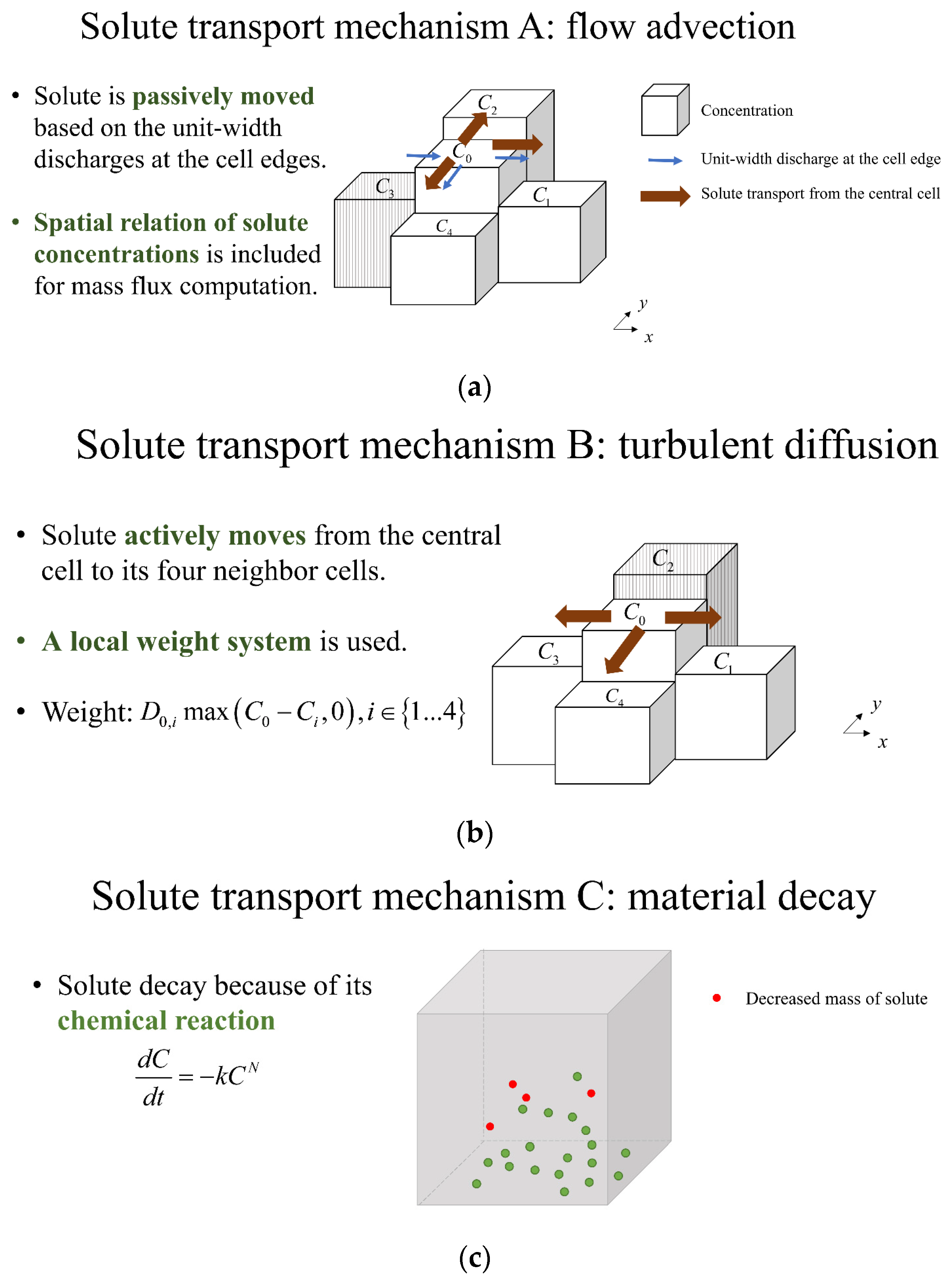
2.3.1. Step 1: Determine the Mass of the Three Mechanisms of Each Central Cell

In this step, the transported mass of the three mechanisms (the flow advection, turbulent diffusion, and material decay mechanisms) for each central cell is determined sequentially, as illustrated in Figure 1a–c, respectively. To avoid the occurrence that the total transported mass from the central cell to its neighbor cells of the three mechanisms exceeds the mass of the central cell, a mass conservation check is also performed in this step. The details for computing the transported mass of the three mechanisms are introduced as follows.
  • Flow advection mechanism
In the flow advection mechanism, the solute is regarded to be passively moved based on the velocity field, as illustrated in Figure 1a. In other numerical models solving the 2D depth-averaged ADEs, numerical difficulties such as numerical diffusion and oscillation are often raised because of the inherent nature of this mechanism to include strong discontinuities from the advection terms ( C · q ), specifically speaking, from C since q come from the given velocity field or a shallow water flow solver. For this, the upwind scheme and the central scheme have been considered in the STMCA approach to calculate C in advection terms due to their simplicity for implementation and relatively less computational demands compared to other more complex schemes. However, the upwind and center schemes suffer from significant numerical diffusion and numerical oscillation, respectively, as already reported by Toro (2001) [35]. To avoid these undesirable numerical diffusions and oscillation, many researchers turn to establishing FV models with the second-order Monotonic Upstream-centered Scheme for Conservation Laws (MUSCL) [2,17,18]. With the help of an appropriate flux limiter, the small variations that often occur near discontinuities at a time step are controlled so that the property of total variation diminishing is preserved. To gain such a desirable ability for effectively handling strong concentration discontinuities, the STMCA approach introduces the use of the flux limiter to consider the spatial relation of solute concentrations for simulating the flow advection mechanism. The developed procedures for computing the transported mass of the flow advection mechanism are described as follows.
First, since the considered solute is passively moved along the velocity field, the transport direction of the solute is judged based on the given unit-width discharge (q = ud or vd) at a cell edge. It is noted that the direction of this unit-width discharge is normal to the corresponding cell edge. If the unit-width discharge of the cell edge is outward from the central cell, the solute of the central cell is moved to the corresponding neighbor cell through the cell edge. As illustrated in Figure 1a, the solute in the central cell can be transported to the 1st, 2nd, and 4th neighbor cells because the given unit-width discharges at the 1st, 2nd, and 4th cell edges are outward from the central cell. After delineating the transport direction of solute, the transported mass through these cell edges is next determined in a general formula as
I i , A d v = q 0 , i C 0 , i Δ t × l
where the subscript Adv refers to the flow advection mechanism, q 0 , i is the given unit-width discharge of the ith cell edge that is computed from a shallow water flow model or given from the velocity field, C 0 , i is the solute concentration at the ith cell edge, Δ t is the adaptive time step, and l is the cell length of the square cell. In Equation (3), I i , A d v has the unit of solute mass (kg) to ensure the mass conservation of solute. To determine C 0 , i , the piecewise slope of the central cell along the direction of the ith cell edge is determined by invoking the Superbee flux limiter since it is recognized to have the highest accuracy in modeling solute transport above other flux limiters [17] (Liang, 2010). To avoid unnecessary computations for the piecewise slopes, for a central cell, the piecewise slope of solute concentration along the x direction ( S 0 , x ) is required to be determined only if the central cell will send out solute through the 1st and/or 3rd cell edge(s). Similarly, the piecewise slope along the y direction ( S 0 , y ) will be computed only if the central cell sends out solute through the 2nd and/or 4th cell edge(s). Taking the computations of C 0 , 1 and C 0 , 3 as an example, S 0 , x is first determined as
S 0 , x = 1 l ϕ r 0 , x C 1 C 0
r 0 , x = C 0 C 3 C 1 C 0
The C 0 , 1 and C 0 , 3 are then computed by
C 0 , 1 = C 0 + 0.5 l × S 0 , x       C 0 , 3 = C 0 0.5 l × S 0 , x
In Equation (4), ϕ r is the adopted flux limiter function (i.e., the Superbee flux limiter in the STMCA approach). S 0 , y , C 0 , 2 , and C 0 , 4 can be computed in a similar way.
2.
Turbulent diffusion mechanism
In this mechanism, the central cell can actively send out solute to the neighbor cells with smaller solute concentrations, as Figure 1b illustrates. Moreover, when the diffusion coefficient is the same, the larger the difference in solute concentrations is, the more the transported solute can be. Similar to the execution of the turbulent diffusion mechanism in Yu and Chang (2022) [34], a local weight system is incorporated to determine the weight of each neighbor cell ( W i , D f )
Δ C i , D f = D 0 , i max C 0 C i , 0   i 1 4
W i , D f = Δ C i , D f Δ C i , D f   i 1 4
in which the word Df refers to the turbulent diffusion mechanism, D 0 , i is the diffusion coefficient along the normal direction of the ith cell edge. The total intercellular mass leaving the central cell ( I t o t , D f ) is decided as
I t o t , D f = min I M , D f W M , D f , I ^ t o t , D f + I t o t , D f p r e
where I M , D f refers to the intercellular mass from the central cell to the neighbor cell with the largest weight ( W M , D f ) as
I t o t , D f = min I M , D f W M , D f , I ^ t o t , D f + I t o t , D f p r e
M is the local index of the neighbor cell with the largest weight ( W M , D f ), W M , D f is the largest value among these weights ( W i , D f ), Δ C M , D f = max Δ C m , D f , and l 2 d 0 is the water volume of the central cell to make the unit of I M , D f become mass. I ^ t o t , D f in Equation (9) is the maximum intercellular mass that will not cause artificial oscillations, which is given by
I ^ t o t , D f = l 2 × min C 0 C i W i d i + 1 d 0   i 1 4
Lastly, I t o t , D f p r e is the intercellular mass that leaves the central cell at the previous time step. After the total intercellular mass leaving the central cell ( I t o t , D f ) is determined, the intercellular mass from the central cell to the ith neighbor cell ( I i , D f ) is subsequently computed as
I i , D f = W i , D f I t o t , D f   i 1 4
3.
Material decay mechanism
In the material decay mechanism, the solute concentration of the central cell is decreased due to the chemical reaction of the solute. Hence, no neighbor cells are involved in determining the decreased mass of the solute at the central cell ( I t o t , D e c a y ), as drawn in Figure 1c. In the STMCA approach, the solute concentration of a computational cell could decay in a N-order reaction (depicted in Equation (2)), and the computation of I t o t , D e c a y is determined by applying the forward Euler method to Equation (2) and multiplying it by the water volume of the central cell as
I t o t , D e c a y = Δ t k C 0 N × l 2 d 0
The letter Decay in the above equation represents the material decay mechanism.
Finally, a mass conservation check is performed to avoid the occurrence of the negative solute concentration. For this, the summation of the transported mass of the three mechanisms ( I t o t ) is computed as i = 1 4 I i , A d v + I t o t , D f + I t o t , D e c a y . Then, when the mass of the central cell ( M 0 = C 0 d 0 l 2 ) is less than I t o t , I i , A d v , I i , D f and I t o t , D e c a y are all multiplied by M 0 / I t o t .

2.3.2. Step 2: Update the Solute Concentration of Each Central Cell

Before updating the solute concentration of each central cell, the STMCA approach will receive the newest velocity field from the adopted shallow water flow model if the velocity field is unsteady. Then, the solute concentration of each central cell is updated by a simple formula as
C 0 = 1 l 2 d 0 C 0 d 0 l 2 i = 1 4 I i , A d v + I i , D f I t o t , D e c a y
where d 0 and C 0 are the water depth and solute concentration of the central cell at the new time stage, respectively.

2.4. Adaptive Time Step and Boundary Conditions

The transition rules introduced in Section 2.3 are all explicit in space and time, thus the Courant–Friedrichs–Lewy and diffusion conditions are applied for determining the adaptive time step ( Δ t ) as
Δ t = min C F L l max u + g d , l 2 8 D
in which u = u 2 + v 2 , CFL refers to the Courant number which is between 0 and 1.
As for the boundary conditions, the STMCA approach supports the assignments of the closed, inlet, and outlet boundary conditions, they are assigned after Step 2 is executed. The closed boundary condition is prescribed by inserting ghost cells with very high solute concentrations around the computational borders. In terms of the inlet boundary condition, the time series of inflowing solute concentration is specified by the user. The solute goes into the computational domain by adding the corresponding solute mass into the central cell where an inlet is located. At the outlet boundaries, a zero gradient of solute concentration is applied at the cell where an outlet is situated.

3. Results and Discussion

This section verifies the accuracy of the proposed STMCA approach in simulating solute transport during pluvial and fluvial floods. In Section 3.1, four idealized cases involving steep gradients of solute concentration/velocity on steady/unsteady flows are adopted to verify the capability of the STMCA approach in handling steep gradients. The flow conditions in these four cases represent commonly seen flow conditions during pluvial and fluvial floods (i.e., regular flows for Case 1, discontinuous flows such as hydraulic jump/drop, and wet-dry interfaces for Cases 2–4). Next, in Section 3.2, the STMCA approach is applied to simulate two idealized pollution events on a real-scale terrain to discover the accuracy and efficiency of the STMCA approach. It is noted that to simulate overland flows and provide the required unit-width discharges for the STMCA approach and FV-TVD solute transport approach, the present study adopts a Godunov-type TVD FV-HLLC model that uses the Minmod flux limiter for its MUSCL scheme [17]. This FV-HLLC model simulates the flows by the same x-y coordinate system as the STMCA approach.

3.1. Model Verification of the STMCA Approach with Four Idealized Solute Transport Cases

First, the capability of the STMCA approach in handling steep concentration gradients without steep velocity gradients is investigated in Case 1 by simulating solute transport in a 2D uniform flow. Two diffusion coefficients are considered to examine the performance of the STMCA approach in advection-dominated and turbulent-dominated conditions. Moreover, the material decay mechanism is considered by using an idealized decay rate and order of the solute reaction. For the next three cases (Cases 2, 3, and 4), in addition to steep concentration gradients, steep gradients of velocity due to strong discontinuities in unsteady flows are also involved. In Case 2, the solute transport along with dam-break flows over a flat plate is simulated. As to the last two cases, they consider dam-break flows over a more complex terrain involving a triangular bump with various downstream and boundary conditions from the CADAM project. Both cases comprise partially reflective waves, hydraulic jumps/drops, and moving wet-dry interfaces, which are commonly seen during pluvial and fluvial floods. In these two cases, a rectangle-shaped concentration profile is considered. The accuracy of the STMCA approach is compared with a commonly used Godunov-type FV solute transport approach with a TVD scheme [17], which is hereinafter referred to be the FV-TVD approach for simplicity. The accuracy of the two approaches is assessed by computing the L2 norms of solute concentration, which is given as
L 2 = C p C ^ p 2 C ^ p 2
in which C p and C ^ p refer to the simulated and exact solute concentrations, respectively.

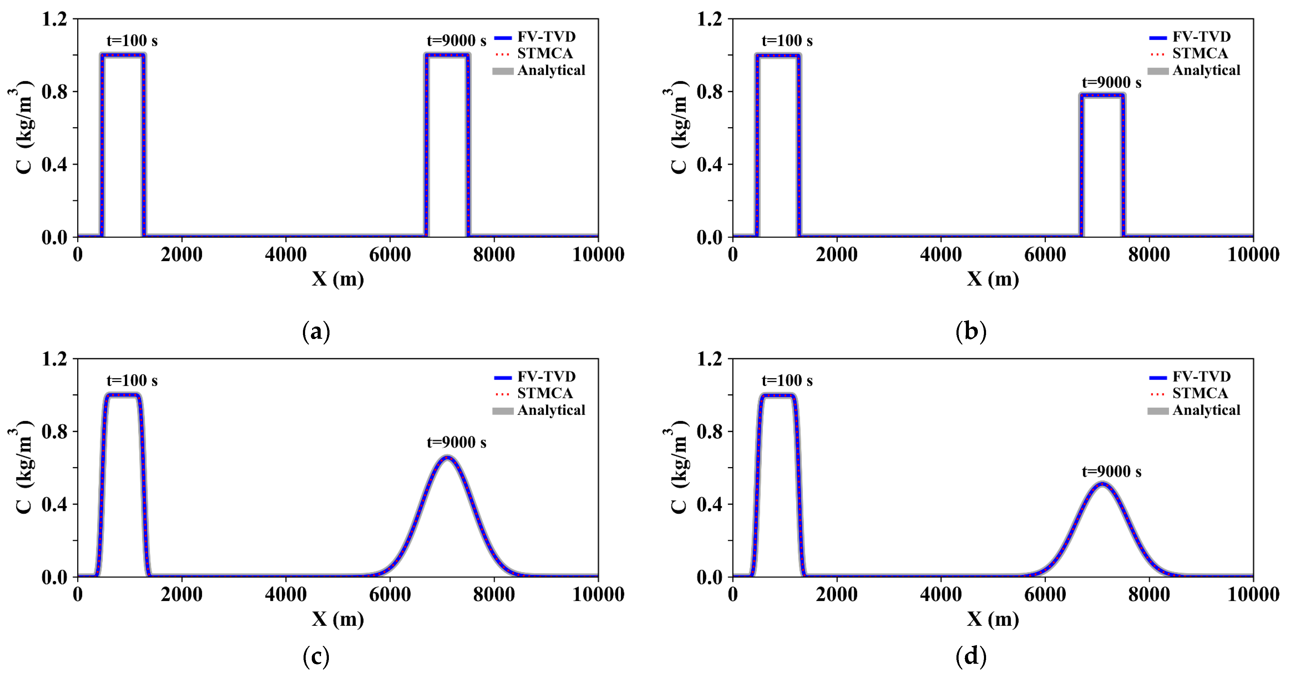
3.1.1. Case 1: Solute Transport in a 2D Uniform Velocity Field (Movement of Solute with Steep Gradients in a 2D Steady Uniform Flow)

Case 1 simulates the solute transport with concentration discontinuities in a horizontal and frictionless rectangle channel that has a length of 10,000 m and a width of 10 m [9]. Concerning the velocity field, a uniform water depth of 0.5 m and water velocities as u = 0.7 m/s and v = 0 m/s are given, and the left and right edges of the computational domain are both prescribed as the transmissive boundary. The computational domain is discretized by a square cell with a length of 2 m, resulting in 25,000 computational cells. In terms of the concentration field, there are four scenarios herein. For all four scenarios, a rectangle-shaped profile (i.e., top hat tracer) with a concentration of 1 kg/m3 is given in a range x 400 800 to form the initial solute concentration profile. A fixed value of the solute concentration of 0 kg/m3 is prescribed at the left and right edges. For the first two scenarios, the time-invariant and uniform diffusion coefficients are both given as 0 m2/s. The second scenario additionally considers the material decay with an order of reaction N = 1 (i.e., the first-order reaction) and decay rate k = 0.1 1/h. As for the subsequent two scenarios, the diffusion coefficient is prescribed as 10 m2/s which leads to a low Péclet number (=0.14). Similarly, the fourth scenario also considers the material decay mechanism with the same values of N and k as the second scenario. Thus, the first two scenarios are both the advection-dominated scenario, and the last two scenarios are both the diffusion-dominated scenario. The simulation durations of all of the relevant simulations are 9000 s to observe the movement of the solute concentration profile. The L2 norm of solute concentration is computed by taking all the simulated solute concentrations in the computational domain when t = 9000 s. The analytical solutions in the advection-dominated scenarios (the first two scenarios) are straightforward since these scenarios are all in the pure advection condition. As to the diffusion-dominated scenarios (the third and fourth scenarios), the analytical solutions can be found in Tian et al. (2022) [36].
The simulated results of the two approaches at t = 9000 s in the four scenarios are drawn in Figure 2a–d, respectively. The simulated results at the beginning time, i.e., t = 100 s, and the analytical solutions are also included in these figures for analysis. Overall, both the STMCA and FV-TVD approaches with/without the material decay mechanism are found to match the analytical solutions well. Moreover, the results of the STMCA approach are almost identical to those of the FV-TVD approach. Hence, the STMCA approach is found to correctly simulate the three mechanisms, and the accuracy of the STMCA approach can be as accurate as the FV-TVD approach both in the advection-dominated and diffusion-dominated scenarios. Specifically, based on the results in the advection-dominated scenario (the first and third scenarios), the STMCA approach has the same ability to handle steep solute concentration gradients as the FV-TVD approach. The L2 norms of solute concentrations are computed and listed in Table 1. From this table, the accuracy of the STMCA approach is confirmed to be the same as the FV-TVD approach in all four scenarios. In summary, the STMCA approach is demonstrated to correctly simulate the three mechanisms in the presence of the discontinuous solute concentration profile on a 2D uniform flow. The accuracy of the STMCA approach is the same as a commonly used Godunov-type FV-TVD approach, which is a satisfactory result.

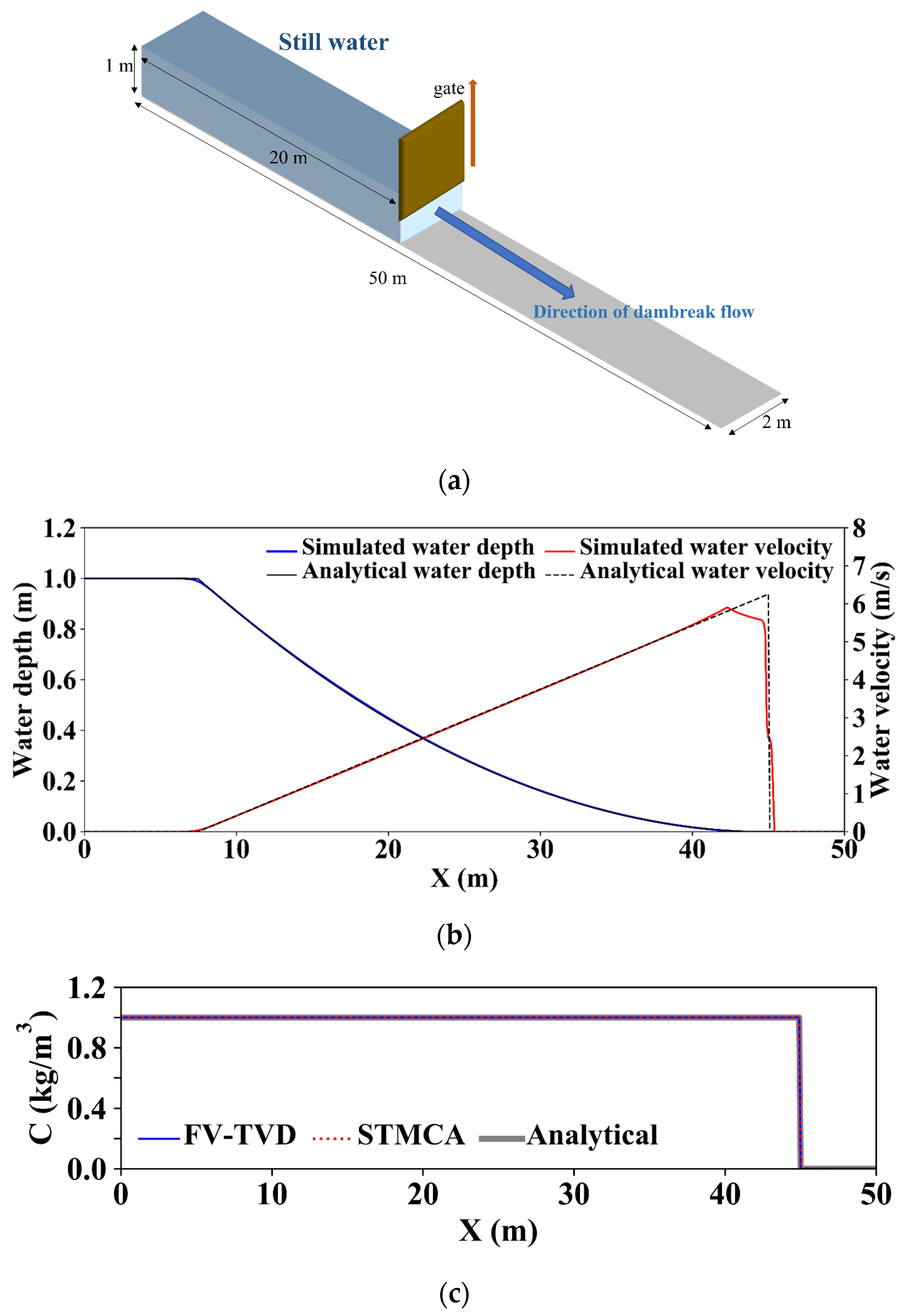
3.1.2. Case 2: Solute Transport in a 2D Dry-Bed Dam-Break Flows over a Horizontal Plate (Solute Transport in an Idealized Dry-Bed Dam-Break Flows)

Case 2 considers a solute concentration discontinuity occurring in a 2D dry-bed dam-break flows on a frictionless and horizontal channel. This 2D unsteady dam-break flow is intensively used to verify various dynamic-wave shallow water flow models and attention is often devoted to the performance near the wet-dry fronts that are the tails of rarefaction waves [35]. The channel has a length of 50 m and a width of 2 m. A gate located at x = 20 m separates the computational domain into left and right reservoirs. In the left reservoir, the initial water depth is given as 1 m and initial water velocities are all 0 m/s. As for the right reservoir, the initial water depth and velocities are all zero. The left and right edges of the computational domain are both prescribed as the transmissive boundary, and the top and bottom edges are both closed. When the simulation begins, the gate disappears immediately, releasing the water from the left reservoir to the right one. Subsequently, transcritical flows with considerably large Froude numbers occur near the wet-dry interfaces that propagate rightward, as Figure 3a depicts. The computational domain is discretized into 10,000 square cells with a fine length of 0.1 m, which is also used by Toro (2001) [35]. For the concentration field, the initial solute concentration in the left and right reservoirs are assigned as 1 kg/m3 and 0 kg/m3, respectively.
The diffusion coefficient is given as 0 m2/s. The simulation lasts for 4 s, and the analytical results of the velocity field are computed using the exact Riemann solver [35]. As for the analytical solute concentration profiles, they can be easily decided as the solute concentrations all equal 1 kg/m3 in wetted computation cells [17]. The simulated solute concentrations when t = 4 s are used to compute the L2 norms of solute concentration for the two studied approaches.
The simulated water depth and velocity profiles at t = 4 s are drawn in Figure 3b to display the simulated velocity field of the adopted FV shallow water flow model. The analytical profiles are also included in this figure. Figure 3b shows that the positions of the moving wet-dry interfaces are accurately captured by the adopted FV shallow water flow model. The analytical and simulated concentration profiles at t = 4 s are displayed in Figure 3c for verification. Inspection of this figure reveals that the two approaches both preserve the sharp solute concentration gradients near the wet-dry interfaces and the simulated results of the STMCA approach are almost the same as the FV approach. The L2 norms of solute concentration at t = 4 s are calculated and listed in Table 1. Again, the STMCA approach is found to be able to achieve almost the same accuracy as the FV-TVD approach. As a result, it is demonstrated that the established transition rules of the STMCA approach can effectively handle the simulations of solute transport in dam-break flows with strong discontinuities in velocity and concentration fields.

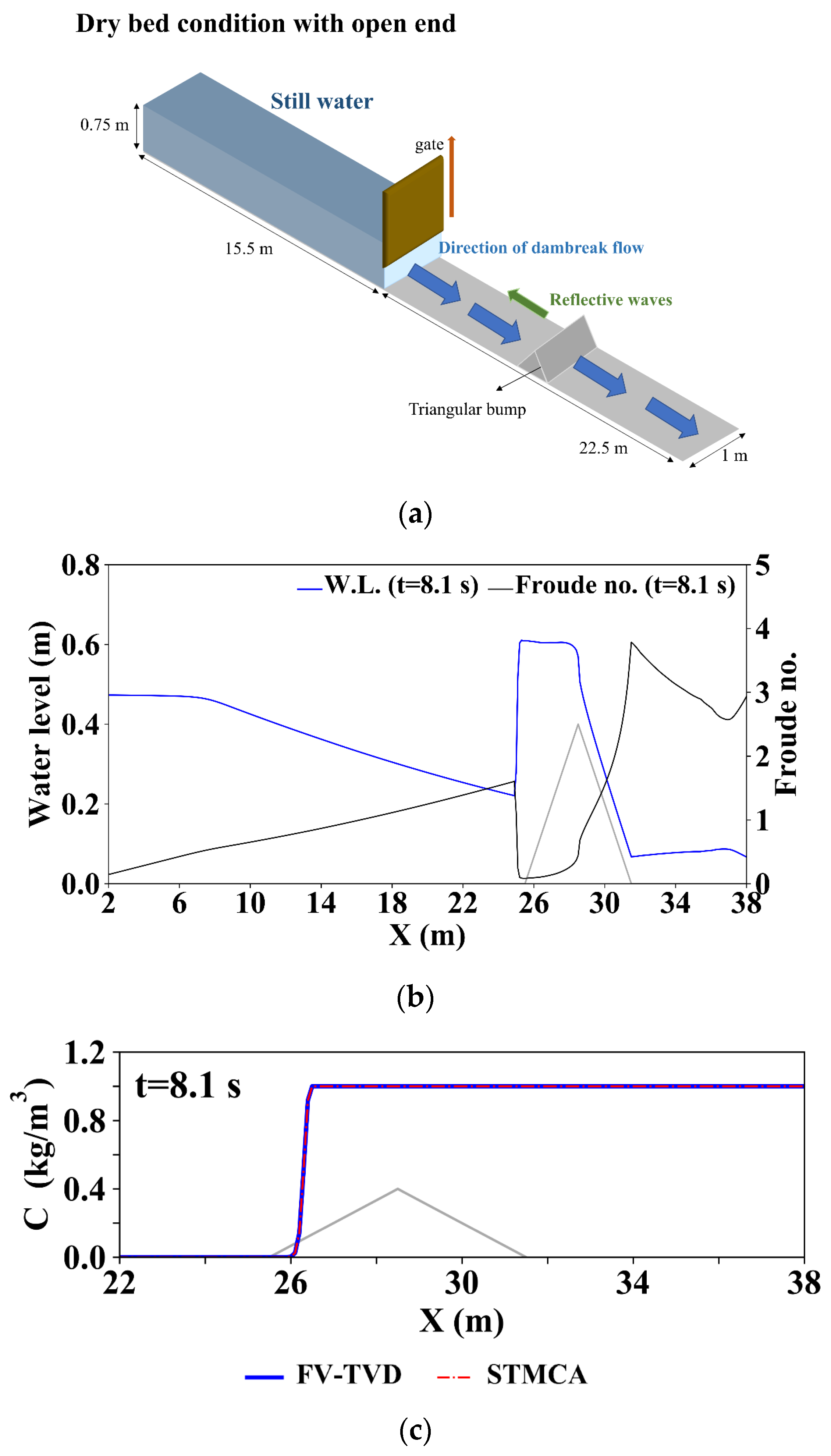
3.1.3. Case 3: Solute Transport in a 2D Dam-Break Flows over a Triangular Bump with the Dry Bed Condition and Open End (Discontinuous Solute Concentrations in a Dam-Break Flow over a Complex Terrain with the Dry Bed Condition and Open End)

In Case 3, more complicated dam-break flows are involved to test the STMCA approach. This dam-break flow case originates from the CADAM project and can be used to discover the ability of a shallow water flow model to handle partially reflective waves, hydraulic jumps/drops, and wet-dry interfaces [3,37,38]. The computational domain comprises a reservoir with a length of 15.5 m and a width of 1.0 m, a rectangular rough channel with a length of 22.5 m and a width of 1.0 m. A gate is placed at the downstream end of the reservoir where x = 15.5 m. A triangular bump with a length of 6.0 m and a height of 0.4 m is located between 22.5 m and 34.5 m. All of the bed elevations except for the triangular bump are zero. Details of the configuration for this case can be found in Chang et al. (2022) [32]. Case 3 is the first scenario among the three scenarios of this CADAM project, i.e., the scenario with the dry bed condition and the open end (depicted in Figure 4a). The Manning roughness coefficient is 0.0125 s/m1/3 in the computational domain. Based on the aforementioned settings, partially reflective waves and hydraulic jumps/drops occurred in the two scenarios, as Figure 4a shows. The computational domain is discretized by square cells with a length of 0.1 m into 4411 cells. From the viewpoint of the solute concentration field, the solute concentration in a range with x coordinates between 13.5 m and 15.5 m is given as 1 kg/m3 to give the initial solute concentration profile. The simulation duration for this case is 40 s. Measured data of the velocity field are provided for verifying the used shallow water flow model. Unfortunately, no analytical solution for solute concentration is provided in this case. Consequently, no L2 norms for solute concentration are computed for the two approaches. The comparison between the two approaches is conducted by taking the simulated concentration profiles at t = 8.1 s.
The water level and Froude number profiles at t = 8.1 s in this scenario are plotted in Figure 4b to display the velocity fields of the case. Inspection of Figure 4b reveals that when the dam-break flows touch the triangular bump, a hydraulic jump occurs as the water level is raised and a partially reflective wave propagates upstream. After the moving wet-dry interfaces pass the bump, the flows turn gradually as the end is open. Concerning the concentration fields, the concentration profiles at t = 8.1 s in the scenario are drawn in Figure 4c for verification. Generally, the STMCA approach is found to obtain very similar results as the FV-TVD approach, which proves the correctness of the STMCA approach in simulating solute concentration under this kind of complex flow condition. Therefore, the STMCA approach has shown its ability to handle steep solute concentration gradients in a velocity field consisting of dam-break flows over irregular terrain.

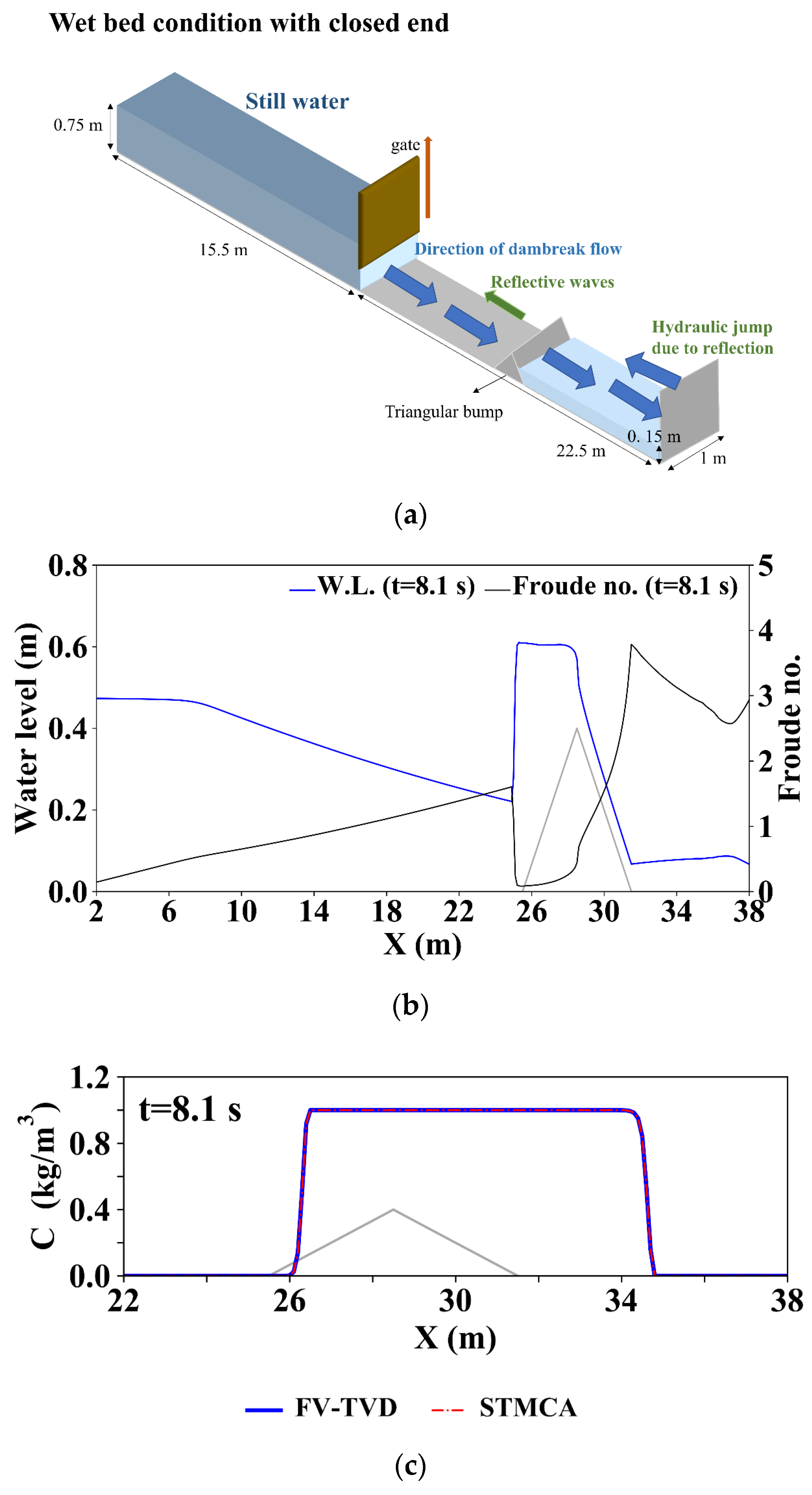
3.1.4. Case 4: Solute Transport in a 2D Dam-Break Flows over a Triangular Bump with the Wet Bed Condition and a Closed End (Discontinuous Solute Concentrations in a Dam-Break Flow over a Complex Terrain with the Wet Bed Condition and a Closed End)

In Case 4, the same configuration as Case 3 is used except for the initial water depth on the channel downstream of the triangular bump, which is given as 0.15 m. Partially reflective waves and hydraulic jumps/drops also occurred in this scenario, as Figure 5a shows. The computational domain is discretized by square cells with a length of 0.1 m into 4411 cells. From the viewpoint of the solute concentration field, the same initial solute concentration profile as Case 3 is used again. The simulation duration for this case is also 40 s. The analytical solution for solute concentration is also absent in this case such that no L2 norm of solute concentration is computed. The comparison between the two approaches is conducted by taking the simulated concentration profiles at t = 8.1 s.
The water level and Froude number profiles at t = 8.1 s in this scenario are plotted in Figure 5b for visualizing the velocity fields. When the dam-break flows touch the triangular bump, a hydraulic jump occurs as the water level is raised and a partially reflective wave propagates upstream. Transcritical flows (i.e., hydraulic jumps) are formed because of the still water in the downstream channel and the closed end. Concerning the concentration fields, the concentration profiles at t = 8.1 s in the scenario are drawn in Figure 5c for verification. Again, the STMCA is found to obtain almost identical results as the FV-TVD approach. In summary, the STMCA approach is demonstrated to be effective in handling the discontinuous solute concentration gradients in various flow conditions.

3.2. Model Applications and Efficiency Assessment on a Real-Scale Terrain

The accuracy of the STMCA approach in steady/unsteady flows with strong concentration gradients has been demonstrated to be as accurate as the FV-TVD approach from Section 3. In Section 4, the STMCA approach is applied to a real-scale terrain with two idealized pollution events. Among various types of pollutants, E. coli which is majorly spread with feces due to flooding is selected as the simulated pollutant. Two pollution scenarios are thus considered according to the cause of flooding, i.e., pluvial or fluvial flooding. A numerical accuracy comparison between the STMCA and FV-TVD approaches is conducted to explore the applicability of the STMCA approach on 2D real-scale terrain. Next, the efficiency improvement of the STMCA approach is evaluated and analyzed.

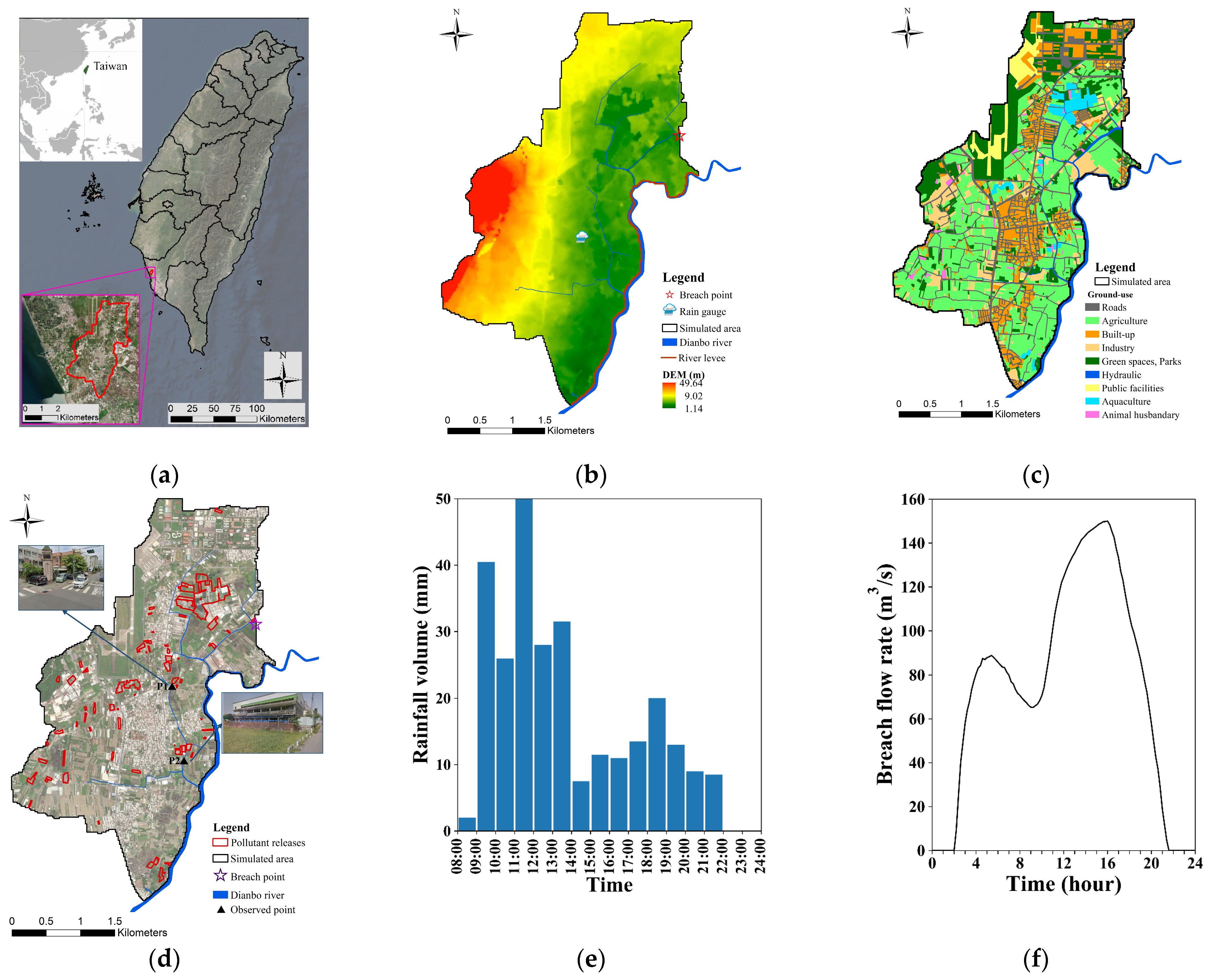
3.2.1. Study Site Delineation

The selected study site is set within the Ziguan District located in the north part of Kaohsiung City, the southern region of Taiwan (Figure 6a). This study site is located in the downstream part of the Dianbo River catchment, as presented in Figure 6b, and a flood levee is built to prevent fluvial flooding from the mainstream of the Dianbo river with a return period of 10 years. Generally, the terrain slopes from west to east, and in the eastern part of the study site the terrain slopes from north to south despite some locally low-lying areas in the northern region. Several tributaries of the Dianbo river pass through and a breach point is set on the tributary that has the largest upstream catchment. The rainfall data of the Ziguan rain gauge (its location is displayed in Figure 6b) is used as the rainfall input for the subsequent simulations. Figure 6c illustrates the land cover of the area, which is primarily covered by agriculture (41%), green spaces and parks (18%), and built-up areas of 16%. The united areas of aquaculture and animal husbandry land use types that could release pollutants during flooding are specified as the pollutant release locations (Figure 6d). A DEM with a 20 m grid resolution is used to describe the terrain, leading to 28,743 square cells for the simulations. The tributaries within the study site are represented by the adopted DEM data. All of the boundaries are closed except for the outlets of these tributaries. The Manning roughness coefficient for each computational cell is determined based on the land-use data. The sewer networks within this study site are ignored since the focus of this manuscript is devoted to developing a novel solute pollutant transport modeling for the shallow water overland flow model.

3.2.2. Pluvial and Fluvial Flood Events

For the pluvial scenario, the rainfall data of a historical 23 August 2018 event that dumped massive rainfall (total amount of 275.5 mm) on the Dianbo catchment within 16 h, as Figure 6e displays. The simulation duration of the pluvial scenario is extended from 16 h to 24 h to let the surface flows gradually recede. Concerning the fluvial scenario, the simulated overbank flow hydrograph near the breach point from the experimental watershed project in Taiwan during the 2016 Typhoon Megi event is reasonably adjusted based on the area of the study site to provide a breach inflow hydrograph, as Figure 6f illustrates. The peak breach inflow rate is 150.0 m3/s at t = 16 h, and the total breach volume within this 24-h breach inflow hydrograph is 32,563,416 m3. The simulation duration for the fluvial scenario is also set as 24 h to let the surface water gradually recede.
In both the two scenarios, E. coli is released from the computational cell that is within the “pollutant releases” regions (Figure 6d) right after the simulated water depth of the cell is greater than 0.3m, which is the water depth threshold that a computational cell is seen to be flooded. The concentrations of the released E. coli for the aquaculture and animal husbandry land-use types are both given as 1000 ppm for demonstration. As for the material decay mechanism of E. coli, the settings in the dairy farm effluent from Craggs et al. (2004) [39] are adopted, i.e., k = 0.02 1/h and N = 1. The anisotropic diffusion coefficients of a computational cell for the two approaches ( D x x for the x direction and D y y for the y direction) are determined by using the proposed formulas by Liang et al. (2010) [2], in which the longitudinal dispersion constant ( ε 1 ) and turbulent diffusion constant ( ε t ) are respectively given as 13.0 and 1.2 (Falconer, 1991) [40]
D x x = n g 1 2 d 5 6 ε 1 u 2 + ε t v 2 u 2 + v 2
D y y = n g 1 2 d 5 6 ε 1 v 2 + ε t u 2 u 2 + v 2
where n is the Manning roughness coefficient of the cell in the shallow water flow model. It is noted that for the STMCA approach, D 0 , 1 = D x x , D 0 , 2 = D y y , D 0 , 3 = D x x , and D 0 , 4 = D y y .

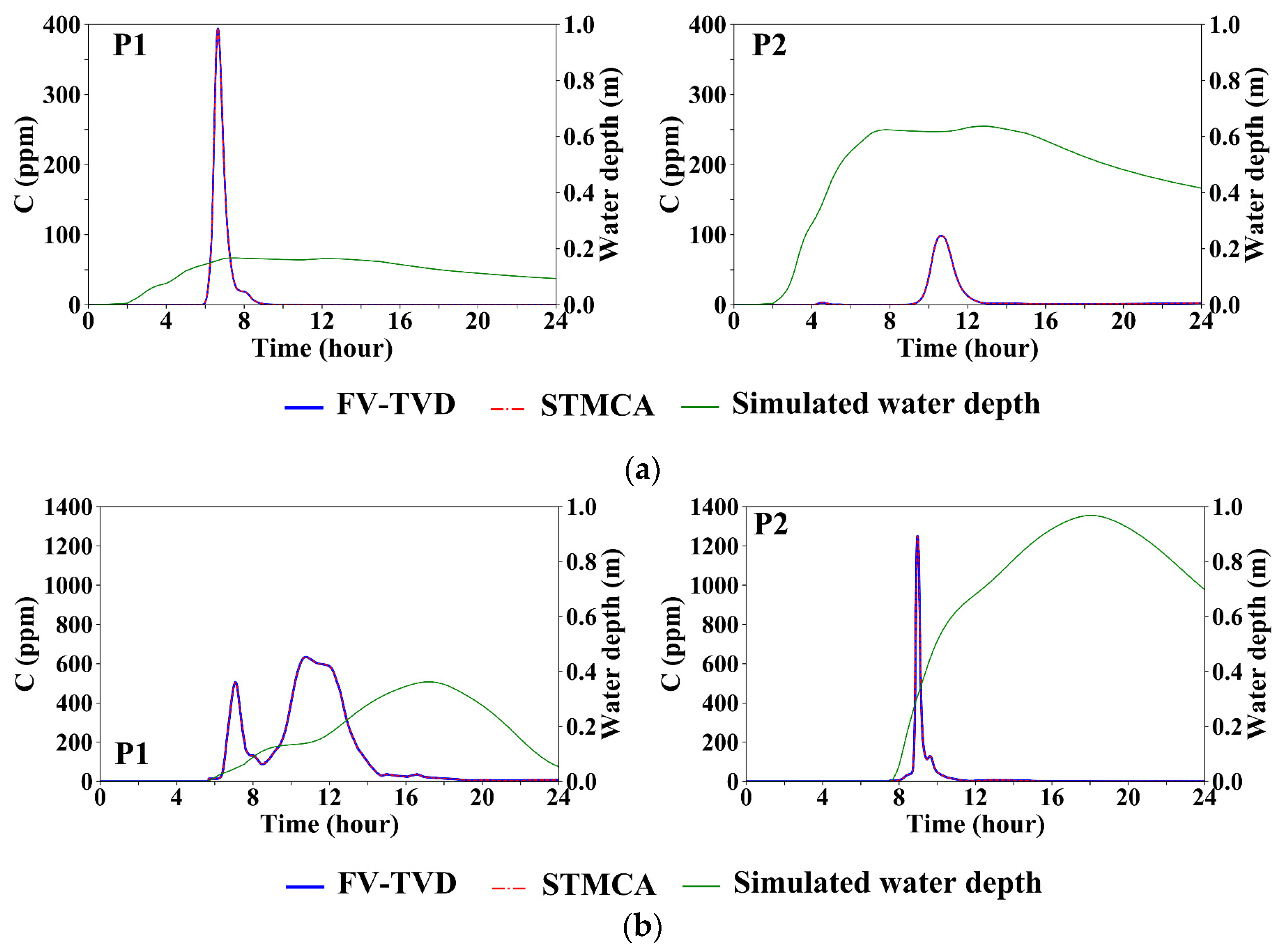
3.2.3. Accuracy Comparison

The accuracy of the two approaches in the pluvial and fluvial scenarios is evaluated by comparing the solute concentration maps that display the peak solute concentration value of each computational cell and the solute concentration hydrographs at two observed points, i.e., P1 and P2, located at the road intersections with essential facilities nearby (locations and street views are drawn in Figure 6d for illustration). The simulated velocity fields of the two scenarios are first introduced since the characteristics of the velocity field play an important role in solute transport modeling. Next, the comparison between the two approaches in the aspect of solute transport modeling is discussed in detail.
4.
Simulated velocity fields
In the pluvial scenario, the simulated flood extent and the simulated flood direction map when t = 25,200 s with the maximum inundation volume are drawn in Figure 7a,b, respectively. From these two figures, the surface runoffs spread over the entire terrain, and inundations occur in low-lying areas of the terrain, i.e., the eastern region, before these runoffs reach the outlets. Relatively higher water velocities are found in areas within the western region with relatively steeper slopes.
As for the fluvial scenario, Figure 7c,d display the simulated flood extent and the simulated flood direction map when t = 63,000 s with the maximum inundation volume, respectively. Compared to the pluvial scenario, the surface runoffs are mostly constrained in the eastern region because of the terrain such that a relatively narrow flood extent with relatively deeper water depths and larger water velocities is seen in this scenario.
5.
Simulated solute concentration fields
The simulated solute concentration maps of the two approaches in the pluvial and fluvial scenarios are displayed in Figure 8a,b, respectively. The regions marked as “pollutant releases” regions are also drawn in these two figures.
In each scenario, the predicted solute concentration maps are also almost the same between the two approaches. In terms of the spatial distribution of E. coli, in both scenarios, relatively high solute concentration is observed around the “pollutant releases” regions that release E. coli into the concentration field and the downstream side of the regions, which is quite reasonable. Nevertheless, it is found that the areas with relatively higher solute concentrations are larger in the fluvial scenario than in the pluvial scenario. Moreover, the released E. coli is found to move further in the fluvial scenario than in the pluvial scenario. The above result is reasonable since the fluvial scenario has relatively larger water velocities than the pluvial scenario. For areas with low water velocities, low solute concentrations are found. Hence, in terms of the solute concentration maps, all two approaches can give acceptable predictions.
From the viewpoint of solute concentration hydrographs, the results of the two scenarios are drawn in Figure 9a,b, respectively. The water depth hydrograph at each observed point is also drawn in the two figures for analysis. Generally, the simulated results of the two approaches are found to be almost identical in both two scenarios. Moreover, in terms of the peaks of solute concentration hydrographs, it is seen that the pluvial scenario has only one peak while the fluvial scenario has more than one peak. Furthermore, the values of peaks in the fluvial scenario are much larger than those in the pluvial scenario. The above result is attributed to the condition that the water velocities are relatively larger in the fluvial scenario than in the pluvial scenario. Hence, based on the above results, the STMCA approach can give reliable results the same as the FV-TVD approach.
In summary, concerning the solute concentration maps and the solute concentration hydrographs, the two approaches provide almost identical and satisfactory results. Moreover, it is seen that in the fluvial scenario with relatively higher water velocities, the pollutants are transported further and quicker into the downstream side along the flow paths than in the pluvial scenario.

3.2.4. Efficiency Assessment

In this subsection, the numerical efficiency of the FV-TVD and STMCA approaches is assessed through the aforementioned pluvial and fluvial scenarios. To accomplish this task, the run times of the two approaches in the pluvial and fluvial scenarios are recorded. The two approaches are all written in the same code structure to minimize the differences in numerical implementation. Moreover, the two approaches are both coded as the dynamic link library (DLL) for the adopted shallow water flow model to access. The subsequent simulations are all conducted on an Intel (R) Core TM i9-9900K PC equipped with 6.0 GB RAM with a clock speed of 3.4 GHz. The STMCA approach is executed without parallel computing to provide a fair comparison with the FV-TVD approach. An equivalent Courant number with a value of 0.2 is used in all the simulations.
The recorded run times of the two approaches are arranged and listed in Table 2 for assessment. As Table 2 lists, the run times of the STMCA approach in the two scenarios are 673 s and 5954 s, respectively, and the FV-TVD approach respectively takes 1949 s and 19,565 s for the two scenarios. Hence, the STMCA approaches are 298.6–328.6% faster than the FV-TVD approach in the two scenarios, which is a satisfactory improvement in the numerical efficiency. This result is attributed to the differences in implementing the flow advection/turbulent diffusion solute transport mechanisms between the FV-TVD approach and the STMCA approach. In the FV-TVD approach, the computations of the advection terms require the extrapolation of solute concentrations at the left-hand and right-hand sides at each cell edge by using the Superbee flux limiter. As to the diffusion terms, they are discretized by the second-order central differencing schemes. Consequently, tedious numerical procedures for computing the relevant gradients and derivatives are introduced. Conversely, for the proposed STMCA approach, simple algebraic equations are used for simulating the flow advection/turbulent diffusion mechanisms [41]. Specifically, the STMCA approach delineates the movement of solute because of the flow advection mechanism by the unit-width discharge before deciding the solute concentration at a cell edge, which subsequently lowers the computations for simulating the flow advection mechanism. Furthermore, a local weight system is incorporated into the simulation of the turbulent diffusion mechanism. As a result, the STMCA approach can outperform the FV-TVD approach by a significant margin. In summary, the STCAM approach is demonstrated to be faster than the FV-TVD approach with almost the same accuracy in simulating solute transport during pluvial and fluvial floods.

4. Conclusions

To provide a more efficient and accurate solute transport modeling during pluvial and fluvial floods, the present study proposes a novel 2D solute transport modeling based on CA framework (STMCA). The STMCA approach uses a set of explicit algebraic equations to simulate the flow advection, turbulent diffusion, and material decay mechanisms in solute transport such that heavy numerical procedures are avoided. The STMCA approach is verified through four cases consisting of steep gradients of solute concentration and velocities with a Godunov-type FV solute transport approach that adopts the TVD scheme to numerically solve the depth-averaged advection-diffusion equations. Next, a real-scale case comprising pluvial/fluvial floods with pollutant transport of E. coli is used for evaluating the numerical accuracy and efficiency of the two solute transport approaches. Based on the simulated results, the following conclusions are drawn.
Overall, the STMCA approach is found to have the same accuracy as the FV approach in idealized and real-scale cases. Specifically, the STMCA approach is demonstrated to handle the discontinuous/steep solute concentration gradient well like the FV approach. Moreover, in the real-scale case, the different characteristics of surface runoffs in the pluvial and fluvial floods are found to subsequently influence the distribution of solute concentration. In the pluvial flood, the water velocities are relatively lower than those of the fluvial flood. Consequently, in the pluvial flood, the released pollutants are mostly situated around the regions that release the pollutants when flooded. By contrast, the released pollutants can pollute to a much greater extent in the fluvial flood. From the viewpoint of efficiency, the STMCA approach can be faster than the FV solute transport approach by 289.6–328.6%, which is a satisfactory efficiency improvement. In summary, this novel STMCA approach is demonstrated to have considerable potential for solute transport modeling.

Author Contributions

Conceptualization, C.-H.W. and H.-L.Y.; methodology, C.-H.W. and H.-L.Y.; software, H.-L.Y.; validation, C.-H.W., H.-L.Y. and T.-J.C.; formal analysis, C.-H.W., H.-L.Y. and T.-J.C.; investigation, C.-H.W., H.-L.Y. and T.-J.C.; resources, C.-H.W.; data curation, C.-H.W. and H.-L.Y.; writing—original draft preparation, C.-H.W. and H.-L.Y.; writing—review and editing, H.-L.Y., C.-H.W. and T.-J.C.; visualization, C.-H.W., H.-L.Y. and T.-J.C.; supervision, C.-H.W. and T.-J.C.; project administration, T.-J.C.; funding acquisition, C.-H.W. and T.-J.C. All authors have read and agreed to the published version of the manuscript.

Funding

The authors are grateful for the financial support of this work partially provided by the National Science and Technology Council, Taiwan, under Grant No. 112-2221-E-002-098-MY3.

Data Availability Statement

The data presented in this study are available on request from the corresponding author.

Conflicts of Interest

The authors declare no conflict of interest.

References

  1. Castro-Orgaz, O.; Hager, W.H. Shallow Water Hydraulics; Springer: Cham, Switzerland, 2019. [Google Scholar]
  2. Liang, D.; Wang, X.; Falconer, R.A.; Bockelmann-Evans, B.N. Solving the depth-integrated solute transport equation with a TVD-MacCormack scheme. Environ. Model. Softw. 2010, 25, 1619–1629. [Google Scholar] [CrossRef]
  3. Kao, H.M.; Chang, T.J. Numerical modeling of dambreak-induced flood and inundation using smoothed particle hydrodynamics. J. Hydrol. 2012, 448–449, 232–244. [Google Scholar] [CrossRef]
  4. Martins, R.; Leandro, J.; Djordjević, S. Wetting and drying numerical treatments for the Roe Riemann scheme. J. Hydraul. Res. 2018, 56, 256–267. [Google Scholar] [CrossRef]
  5. Bai, F.P.; Yang, Z.H.; Zhou, W.G. Study of total variation diminishing (TVD) slope limiter in dam-break flow simulation. Water Sci. Eng. 2018, 11, 68–74. [Google Scholar] [CrossRef]
  6. Yu, H.L.; Chang, T.J. A hybrid shallow water solver for overland flow modelling in rural and urban areas. J. Hydrol. 2021, 598, 126262. [Google Scholar] [CrossRef]
  7. Zhao, J.; Liang, Q. Novel variable reconstruction and friction term discretization schemes for hydrodynamic modelling of overland flow and surface water flooding. Adv. Water Resour. 2022, 163, 104187. [Google Scholar] [CrossRef]
  8. Ferrari, A.; Vacondio, R.; Dazzi, S.; Mignosa, P. A 1D-2D Shallow Water Equations solver for discontinuous porosity field based on a Generalized Riemann Problem. Adv. Water Resour. 2017, 107, 233–249. [Google Scholar] [CrossRef]
  9. Chang, Y.S.; Chang, T.J. SPH simulations of solute transport in flows with steep velocity and concentration gradients. Water 2017, 9, 132. [Google Scholar] [CrossRef]
  10. Guan, Y.; Altinakar, M.S.; Krishnappan, B.G. Two-dimensional simulation of advection-dispersion in open channel flows. In Proceedings of the 5th International Conference on Hydro-Informatics, Cardfiff, UK, 1–5 July 2002; pp. 226–231. [Google Scholar]
  11. Yeh, G.T.; Chang, J.R. An exact peak capturing and oscillation-free scheme to solve advection-dispersion transport equations. Water Resour. Res. 1992, 28, 2937–2951. [Google Scholar] [CrossRef]
  12. Lee, M.E.; Seo, I.W. Analysis of pollutant transport in the Han River with tidal current using a 2D finite element model. J. Hydro-Environ. Res. 2007, 1, 30–42. [Google Scholar] [CrossRef]
  13. Ginzburg, I.; Roux, L.; Silva, G. Local boundary reflections in lattice Boltzmann schemes: Spurious boundary layers and their impact on the velocity, diffusion and dispersion. C. R. Mec. 2015, 343, 518–532. [Google Scholar] [CrossRef]
  14. Wang, H.; Cater, J.; Liu, H.; Ding, X.; Huang, W. A lattice Boltzmann model for solute transport in open channel flow. J. Hydrol. 2018, 556, 419–426. [Google Scholar] [CrossRef]
  15. Murillo, J.; García-Navarro, P.; Burguete, J. Analysis of a second-order upwind method for the simulation of solute transport in 2D shallow water flow. Int. J. Numer. Meth. Fluids 2008, 56, 661–686. [Google Scholar] [CrossRef]
  16. Burguete, B.; García-Navarro, P.; Murillo, J. Preserving bounded and conservative solutions of transport in one-dimensional shallow-water flow with upwind numerical schemes: Application to fertigation and solute transport in rivers. Int. J. Numer. Meth. Fluids 2008, 56, 1731–1764. [Google Scholar] [CrossRef]
  17. Liang, Q. A well-balanced and non-negative numerical scheme for solving the integrated shallow water and solute transport equations. Commun. Comput. Phys. 2010, 7, 1049–1075. [Google Scholar] [CrossRef]
  18. Zhang, L.; Liang, Q.; Wang, Y.; Yin, J. A robust coupled model for solute transport driven by severe flow conditions. J. Hydro-Environ. Res. 2015, 9, 49–60. [Google Scholar] [CrossRef]
  19. Morales-Hernánez, M.; Murillo, J.; García-Navarro, P. Diffusion-dispersion numerical discretization for solute transport in 2D transient shallow flows. Environ. Fluid Mech. 2019, 19, 1217–1234. [Google Scholar] [CrossRef]
  20. Lin, L.; Liu, Z. TVDal: Total variation diminishing scheme with alternating limiters to balance numerical compression and diffusion. Ocean Model. 2019, 134, 42–50. [Google Scholar] [CrossRef]
  21. Herrera, P.A.; Massabó, M.; Beckie, R.D. A meshless method to simulate solute transport in heterogeneous porous media. Adv. Water Resour. 2009, 32, 413–429. [Google Scholar] [CrossRef]
  22. Park, I.; Seo, I.W. Modeling non-Fickian pollutant mixing in open channel flows using two-dimensional particle dispersion model. Adv. Water Resour. 2018, 111, 105–120. [Google Scholar] [CrossRef]
  23. Sämann, R.; Graf, T.; Neuweiler, I. Modeling of contaminant transport during an urban pluvial flood event-the importance of surface flow. J. Hydrol. 2019, 568, 301–310. [Google Scholar] [CrossRef]
  24. Liu, W.; Hou, Q.; Lian, J.; Zhang, A.; Dang, J. Coastal pollutant transport modeling using smoothed particle hydrodynamics with diffusive flux. Adv. Water Resour. 2020, 146, 103764. [Google Scholar] [CrossRef]
  25. Hou, J.; Liang, Q.; Li, Z.; Wang, S.; Hinkelmann, R. Numerical error control for second-order explicit TVD scheme with limiters in advection simulation. Comput. Math. Appl. 2015, 70, 2197–2209. [Google Scholar] [CrossRef]
  26. Wolfram, S. Cellular automata as models of complexity. Nature 1984, 311, 419–424. [Google Scholar] [CrossRef]
  27. Chang, T.J.; Yu, H.L.; Wang, C.H.; Chen, A.S. Overland-gully-sewer (2D-1D-1D) urban inundation modeling based on cellular automata framework. J. Hydrol. 2021, 603, 127001. [Google Scholar] [CrossRef]
  28. Hadeler, K.P.; Müller, J. Cellular Automata: Analysis and Applications; Springer: Cham, Germany, 2017. [Google Scholar]
  29. Dottori, F.; Todini, E. Developments of a flood inundation model based on the cellular automata approach: Testing different methods to improve model performance. Phys. Chem. Earth Parts ABC 2011, 36, 266–280. [Google Scholar] [CrossRef]
  30. Ghimire, B.; Chen, A.S.; Guidolin, M.; Keedwell, E.C.; Djordjević, S.; Savić, D.A. Formulation of a fast 2D urban pluvial flood model using a cellular automata approach. J. Hydroinformatics 2013, 15, 676. [Google Scholar] [CrossRef]
  31. Guidolin, M.; Chen, A.S.; Ghimire, B.; Keedwell, E.C.; Djordjević, S.; Savić, D.A. A weighted cellular automata 2D inundation model for rapid flood analysis. Environ. Model. Softw. 2016, 84, 378–394. [Google Scholar] [CrossRef]
  32. Chang, T.J.; Yu, H.L.; Wang, C.H.; Chen, A.S. Dynamic-wave cellular automata framework for shallow water flow modeling. J. Hydrol. 2022, 613, 128449. [Google Scholar] [CrossRef]
  33. Milašinović, M.; Ranđelović, A.; Jaćimović, N.; Prodanović, D. Coupled groundwater hydrodynamic and pollution transport modelling using Cellular Automata approach. J. Hydrol. 2019, 576, 652–666. [Google Scholar] [CrossRef]
  34. Yu, H.L.; Chang, T.J. Modeling particulate matter concentration in indoor environment with cellular automata framework. Build Environ. 2022, 214, 108898. [Google Scholar] [CrossRef]
  35. Toro, E.F. Shock-Capturing Methods for Free-Surface Shallow Flows; John Wiley: New York, NY, USA, 2001. [Google Scholar]
  36. Tian, L.; Gu, S.; Wu, Y.; Wu, H.; Zhang, C. Numerical investigation of pollutant transport in a realistic terrain with the SPH-SWE method. Front. Environ. Sci. 2022, 10, 889526. [Google Scholar] [CrossRef]
  37. Zhou, J.G.; Causon, D.M.; Mingham, C.G.; Ingram, D.M. Numerical prediction of dam-break flows in general geometries with complex bed topography. J. Hydrau. Eng. ASCE 2004, 130, 332–340. [Google Scholar] [CrossRef]
  38. Chang, T.J.; Kao, H.M.; Chang, K.H.; Hsu, M.H. Numerical simulation of shallow-water dam break flows in open channels using smoothed particle hydrodynamics. J. Hydrol. 2011, 408, 78–90. [Google Scholar] [CrossRef]
  39. Craggs, R.J.; Zwart, A.; Nagels, J.W.; Davies-Colley, R.J. Modelling sunlight disinfection in a high rate pond. Ecol. Eng. 2004, 22, 113–122. [Google Scholar] [CrossRef]
  40. Falconer, R.A.; Chen, Y. An improved representation of flooding and drying and wind stress effects in a two-dimensional tidal numerical model. Proc. Inst. Civ. Eng. 1991, 91, 659–678. [Google Scholar] [CrossRef]
  41. Chopard, B. Cellular Automata Modeling of Physical Systems. In Encyclopedia of Complexity and Systems Science, 1st ed.; Meyers, R.A., Ed.; Springer: Greer, SC, USA, 2009; pp. 856–892. [Google Scholar]
Figure 1. The schematic illustrations of the simulations of the three mechanisms. (a) The flow advection mechanism; (b) The turbulent diffusion mechanism; (c) The material decay mechanism. The green and red dots respectively represent the kept and decreased solutes.
Water 16 00129 g001
Figure 2. The comparison of the analytical and simulated results when t = 100 s and 9000 s in Case 1. (a) The result when D = 0 m2/s; (b) The result when D = 0 m2/s with the material decay; (c) The result when D = 10 m2/s; (d) The result when D = 10 m2/s with the material decay. The material decay is given as a first-order reaction (N = 1) with k = 0.1 1/h.
Water 16 00129 g002
Figure 3. The solute transport in a 2D dam-break flows on a frictionless and flat terrain (Case 2). (a) The illustration of the case; (b) The simulated water depth and velocity profiles when t = 4 s; (c) The comparison between the STMCA and FV-TVD approaches when t = 4 s.
Water 16 00129 g003
Figure 4. The solute transport in a 2D dam-break flows over a triangular bump under the dry bed condition with an open end (Case 3). (a) The illustration of the case; (b) The simulated water level and Froude number profiles when t = 8.1 s; (c) The comparison between the STMCA and FV-TVD approaches when t = 8.1 s.
Water 16 00129 g004
Figure 5. The solute transport in a 2D dam-break flows over a triangular bump under the wet bed condition with a closed end (Case 4). (a) The illustration of the case; (b) The simulated water level and Froude number profiles when t = 8.1 s; (c) The comparison between the STMCA and FV-TVD approaches when t = 8.1 s.
Water 16 00129 g005
Figure 6. Model application and efficiency assessment on a real-scale terrain in Taiwan. (a) The location of the study site; (b) The surface elevation, and locations of the Ziguan rain gauge and breach point; (c) The land-use map and the regions of “pollutant releases”; (d) The locations of the two observed points for comparing the solute concentration hydrographs between the two approaches; (e) The input rainfall data of the Ziguan rain gauge on the 23 August 2018 event for the pluvial scenario. (f) The input breach inflow hydrograph that is derived by using the simulated overbank flow hydrograph near the breach point from the experimental watershed project for the 2016 Typhoon Megi event for the fluvial event.
Water 16 00129 g006
Figure 7. (a) The simulated flood extent of the pluvial event; (b) The simulated flood direction map when t = 25,200 s (with the maximum inundation volume) of the pluvial event; (c) The simulated flood extent of the fluvial event; (d) The simulated flood direction map when t = 63,000 s (with the maximum inundation volume) of the fluvial event.
Water 16 00129 g007
Figure 8. The simulated solute concentration maps of the STMCA and FV-TVD approaches in the two scenarios. (a) The pluvial scenario; (b) The fluvial scenario.
Water 16 00129 g008
Figure 9. The comparison of the solute concentration hydrographs at the two observed points between the two approaches in the pluvial and fluvial scenarios. (a) The pluvial scenario; (b) The fluvial scenario.
Water 16 00129 g009
Table 1. The numerical accuracy of the STMCA and FV-TVD approaches in Cases 1 and 2 with analytical solutions. The L2 norm for solute concentration is used for the comparison.
CaseScenarioThe STMCA ApproachThe FV-TVD Approach
Case 1D = 0 m2/s0.031660.03166
D = 0 m2/s with the material decay0.031660.03166
D = 10 m2/s0.002480.00248
D = 10 m2/s with the material decay0.002480.00248
Case 2-<0.00001<0.00001
Table 2. The efficiency comparison between the STMCA and FV-TVD approaches in the real-scale case.
FloodThe Run Time of the FV-TVD Approach (s)
(1)
The Run Time of the STMCA Approach (s)
(2)
The Efficiency Enhancement of the STMCA Approach (%)
(3) = (1)/(2)
Pluvial1949673289.6%
Fluvial19,5655954328.6%
Disclaimer/Publisher’s Note: The statements, opinions and data contained in all publications are solely those of the individual author(s) and contributor(s) and not of MDPI and/or the editor(s). MDPI and/or the editor(s) disclaim responsibility for any injury to people or property resulting from any ideas, methods, instructions or products referred to in the content.

