Impact of Climate Change on the Water Balance of the Akaki Catchment

Abstract

Climate change has an impact on water resources. Estimations of the variations in water balance under climate change variables are essential for managing and developing the water resource of a catchment. The current investigation evaluated the magnitude of the change in the water balance component of the Akaki catchment, Ethiopia, using the semi-distributed hydrological model, the Soil and Water Assessment Tool (SWAT), with the integration of the Coordinated Regional Downscaling Experiment of Africa under RCP4.5 and 8.5. The SWAT model was developed using spatial and temporal data; it was calibrated (1991–2001) and validated (2002–2004) using SWAT-CUP. The statistical monthly SWAT model performance values of the NSE, PBIAS (%), and R² showed good agreement between calibration and validation. On an annual basis, projected rainfall is expected to increase by 14.96%, 4.13%, 8.39%, and 10.39% in the 2040s under RCP4.5 and 8.5 and in the 2060s under RCP4.5 and 8.5, respectively, with inconsistent change on a monthly projections basis for each scenario. The projected monthly and yearly temperatures are expected to increase under different climate change scenarios. Annual evapotranspiration and potential evapotranspiration increased under both RCPs, whereas surface runoff, lateral flow, and water yield declined under the climate scenarios of each RCP. Monthly projected water yield showed a non-uniform change in the first 30 years and in the second years under the RCP4.5 and RCP8.5 scenarios. These results show that the catchment is highly vulnerable to hydrological and agricultural drought due to water availability. These research findings provide valuable evidence on the role of climate change in water balance, which will help decision makers to achieve better water resource management.

1. Introduction

The significant impact of climate change has resulted from changes in the average temperature and precipitation over a specified area over the long term [1]. Concern about climate change has recently declined and has become a surprise issue for academic communities. Increased atmospheric carbon dioxide (CO₂) and associated greenhouse gas emissions are leading causes of warming trends, higher surface temperatures on Earth, and concurrent changes in precipitation regimes [2,3]. The rapid expansion of urban areas and the growth of industrial stages from time to time in various locations at the national and international levels have resulted in major disruption to the climate system due to the rising concertation of greenhouse gases. Global warming will be one of the most challenging problems for humans in 2100 [4,5]. Warmer and colder climates will speed up the alteration of water resource availability by shifting the intensity and duration of rainfall and the degree and timing of runoff. Climate change occurrence and intensity affect the water balance [6,7,8,9].

To effectively manage catchment water resources, it is imperative to assess the effects of global climate change at the catchment level from the perspective of socioeconomic development [5]. The vulnerability of water resources to climate change components enforces the prediction of climate variability for the estimation of future variants in the water cycle [10,11,12]. Therefore, the evaluation of the impact of climate change on hydrology and water resources is essential for sustainable planning and operations to balance water supply and demand for irrigation, energy production, and infrastructures [13,14]. The impact of climate change on water resources and the need to adapt to the existing circumstances regarding changes in hydrologic components that could occur because of climate change within the catchment are hot issues in the hydrology and water resource discipline [3,15,16,17]. With changes in temperature and rainfall, climate change has accelerated changes in the quantity of water balance elements and affected river water resources. However, because of the location of these resources in different topographies and the geological conditions of catchments, hydrologic component responses to precipitation and temperature may not be similar [18,19,20]. Temperature changes linked to human activities cause climate variation, affecting surface and groundwater availability by altering humidity in the atmosphere, rotation, rainfall, soil water holding capacity, and runoff. This accelerates the change in the catchment water cycle by increasing evaporation [10,21,22]. To suggest a scientific policy to minimize such problems in water sectors, in earlier investigations, scholars applied regional climate models to analyze the impact of climate change on hydrology and water resources worldwide [23,24,25,26]. Changes in water balance quantity and quality of river basins, lakes, catchment, and watershed scales from regional to continental due to changes in air temperature were confirmed using a hydrological model under different climate scenarios [27,28,29]

The National Meteorological Agency (2001) discovered that climate variability and change in Ethiopia mainly manifest through variability, a decreasing trend in rainfall, and an increasing trend in temperature. Additionally, as cited in [1], the Intergovernmental Panel on Climate Change (IPCC) reported that the mean annual temperature in mid-emission scenarios will increase to a range from 0.9 °C to 1.1 °C, 1.7 °C to 2.1 °C, and 2.7 °C to 3.4 °C by the end of 2030, 2050, and 2080, respectively, compared with the mean yearly temperature from 1961 to 1990, and the average annual temperature amplified by 1.3 °C from 1960 to 2006, which is 0.28 °C per year in Ethiopia. In the country, greenhouse gas emission sources include deforestation, agriculture, land use, transport, electricity, industry, and buildings [1]. Understanding the multifaceted connections among climate schemes, terrestrial systems, and human systems is vital for forecasting river water balance responses to climate change and executing sustainable water use management in Ethiopia. Under climate change, the water balance components of a river basin change irregularly, and the Awash River basin is evidence of this.

Nevertheless, the negative and positive rates of evolution of river basins differ due to their location in different topographic and geological conditions and ecological features. Because of these natural factors, rainfall and temperature patterns significantly change in the Awash River basin. Climate change is expected to raise water problems by affecting the hydrological process of the Awash basin [28]. As a result, the amount and seasonality of the water supply are projected to shifts because of the change in the precipitation and temperatures. In this research, we used Coordinated Regional Climate Downscaling Experiment (CORDEX) output variables with the integration of the Soil and Water Assessment Tool (SWAT) to evaluate the effects of climate change on the water balance component of the Akaki catchment. The SWAT model is one of the most vital hydrological models used to enumerate the outcome of climate change on the water balance component of a catchment. Many scholars have effectively applied the CORDEX output and the SWAT model in the river basin in recent decades in Ethiopia [30,31,32]. The main goal of this study was to provide scientific information concerning the effective development of water resources at the catchment level and the link between rainfall and climate change, which could provide essential information for integrated catchment water resource planners, managers, policy makers, and the regional community. Evaluating the water balance component in the catchment under climate change is a precondition in developing evidence-based water management. This study produced climate change scenarios for 2026–2055 (the 2040s) and 2056–2085 (the 2060s). In this investigation, the effect of land use/cover change on the water balance was assumed to be constant. Sediment yield response to climate change in the Akaki catchment was not assessed.

2. Materials and Methods

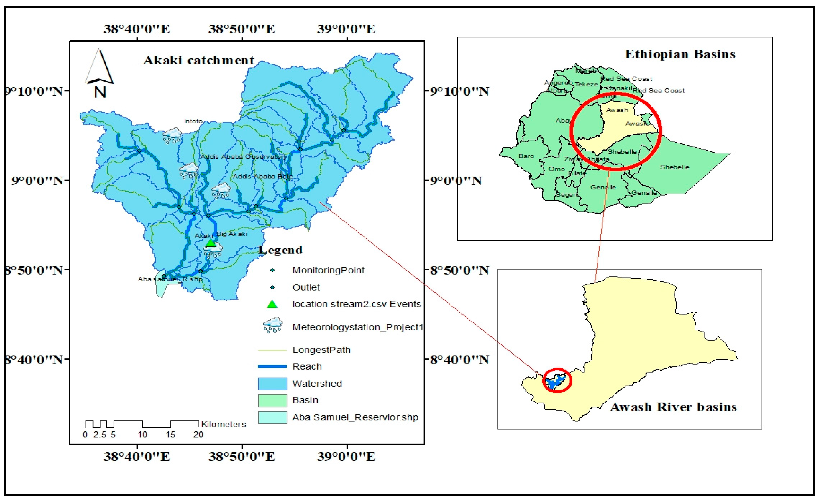
2.1. Description of the Study Area

The Akaki catchment (Figure 1) is located in central Ethiopia. Its latitude and longitude boundaries are 8°50′00″–9°10′00″ N and 38°35′00″–39°5′00″ E, respectively. The drainage area of the Akaki catchment is 1468 km². The Little and Great Akaki watersheds are the main two sub-basins of the Akaki River and join together at the Aba-Samuel reservoir. The catchment receives high rainfall in June, July, August, and September; and less rainfall in mid-February, March, and April. The highest average monthly precipitation between 1988 and 2017 was measured in August at 278.5 mm. The lowest mean monthly rainfall was 9 mm in November, with approximately 1114.9 mm mean annual rainfall; according to data collected from the National Meteorological Agency, the minimum rainfall recorded in 1997 was 904.28 mm, and the highest in 1996 was 1450.43 mm. The mean monthly maximum temperature oscillates between 21 and 25 °C, and the minimum temperature varies from 7 to 11 °C. During the same period, the lowest temperatures were recorded in July and August, while the highest were recorded in February and March. In the Akaki watershed, 361 Hydrologic Responses Units (HRUs) were created with 29 sub-watersheds. The catchment is mostly dominated by agricultural land use. The elevation of the Akaki catchment varies from 1989 m to 3368 m above mean sea level. The highest and lowest elevation ranges are the northern ridges and the southernmost parts of the catchment.

2.2. Data Used

The SWAT model needs spatial and temporal data to simulate water balance components under baseline and future climate data. Accordingly, the digital elevation map, land use/cover (Figure 2), the soil map (Figure 3), hydrological data (streamflow), and meteorological data were obtained from the United States Government Survey (USGS), the Department of GIS (Geography Information System), Department of Hydrology, the Ministry of Water and Energy of Ethiopia, and the National Meteorological Agency, respectively. The CORDEX of Africa project provided the SMHI.ICHEC-EC EARTH. r1i1p1. RCA4 model with the historical and future RCP 4.5 and 8.5. RCP4.5 and RCP8.5 represent the concentration of carbon dioxide transfers in global warming at a mean of 4.5 (medium emission) and 8.5 (higher emission) watts per square meter across the planets, respectively. Downscaled climate data from different domains of the CORDEX of the regional climate model were applied to evaluate the impact of climate change on water balance worldwide [33,34,35,36,37].

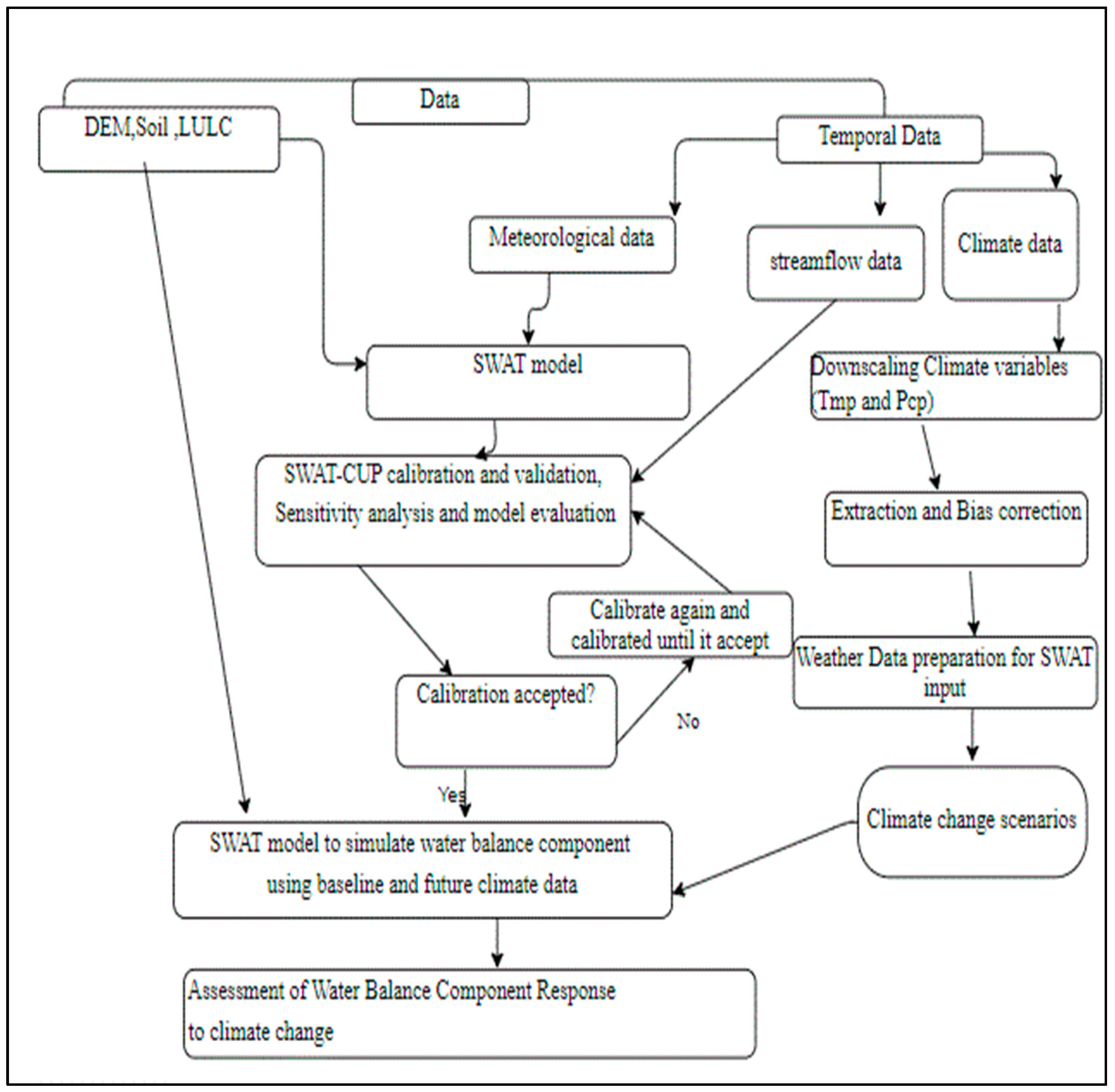
3. Performed Methodology

3.1. The Hydrologic Model

A hydrologic model is a frequent term described by a mathematical depiction of the hydrologic processes of a catchment. Many hydrologic models have been developed from lumped models to fully distributed models based on a process. There is a range of possible model structures within each type of hydrological model. Hence, selecting a particular model for a specific application, like climate change modeling, is a challenge for the model user community. Data accessibility and the objective of the study influence the hydrological model to be chosen. Accordingly, based on data and model availability, this research used a physical-based hydrological model named the SWAT model to simulate monthly water balance using baseline and future climate data. This model was successfully applied in simulating water balance in different basins—for instance, in the Congo River Basin [38], to simulate the hydrologic regime under RCP4.5 and RCP8.5, in the evaluation of water resources response to climate change in the Diyala River Basin, Iraq, and in the Dokan Dam watershed, Iran [39,40] and [41] in the Heeia watershed in Hawaii to assess water component responses to climate change. One of the primary purposes of the SWAT model is to estimate the hydrological process of watersheds in big or small areas and assess the impact of climate change in the environment. In this study, potential evapotranspiration was calculated by using the Hargreaves method. This approach uses temperature as an input for potential evapotranspiration computation use. The potential evapotranspiration was calculated using Equation (1), which was original developed in [42] and reported in the SWAT model document [43].

$${\lambda E_O=0.0023H_0\left(Tmax-Tmin\right)}^{0.5}\left(Tav+17.8\right)$$

(1)

In the above Equation (1) λ is the latent heat of vaporization in megajoule per kilogram (M.J/KG), Eo is potential evapotranspiration in millimeter per day, $H_0$ is the extraterrestrial radiation in megajoule per meter square per day (MJ/m²d), Tmax is the maximum temperature in a given day in °C, Tmin is the minimum air temperature for a given day in °C, and $Tav$ is the mean air temperature for a given day in °C.

3.2. Model Calibration and Validation

SWAT model calibration and verification are required to calibrate and validate the model using river flow before the model is used to estimate the hydrologic process and climate change effect analysis on the water balance of a catchment. It is essential to highlight that the hydrological model does not recognize the initial simulation situations. These situations can significantly influence the pretend process and need a warm-up period. Calibration is a mechanism to adjust the model parameter range to enhance model workability depending on an interval of prelimited principles in the SWAT model. Also, it is a process used to reduce the difference between simulated and observed river discharge [44]. Validation is a step of running a model with the parameters determined during the calibration process with a dataset not used for calibration. It builds confidence in whether the model accurately represents the actual system. Calibration and validation of hydrological models are critical in assessing hydrological model performance in simulating catchment hydrology [45]. In this work, SUFI-2 was selected to analyze sensitive parameters. The SUFI-2 program is mainly used in sensitivity analysis, calibration, and validation. The initial step in the SWAT model calibration and validation procedure would be to choose the most sensitive parameters for a specific catchment [46]. This study set the global sensitivity method to select the most sensitive parameters during calibration [47,48,49,50].

3.3. Hydrologic Model Performance Evaluation

Model performance was evaluated using the coefficient of determination (R²), the Nash–Sutcliffe Efficiency (NSE), the percent bias PBIAS), and the graphical relationship, which determines the quality of goodness of fit and reliability of the simulated streamflow to observed streamflow values. The ability of the SWAT model to simulate the water balance component was evaluated based on monthly time series, and the Nash–Sutcliffe Efficiency (NSE) was selected as the objective function. The coefficient of determination (R²) measures how well the model replicates observed outcomes. The range of R² lies between 0 and 1, which describes how much of the observed desperation is explained by the prediction (Equation (2)). A zero value means no correlation between recorded and modeled discharge during calibration and validation of the hydrological model, which is not acceptable for the model performance indication. In contrast, one means the desperation of the model is equal to that of the observation. But in the real world for the hydrological model, the value of the coefficient of determination might not be one due to uncertainty from the modeler, data, model, and other factors. The Nash–Sutcliffe Efficiency ranges from −∞ to 1 [51], in which the NSE equal to one corresponds to a perfect match of modeled discharge with the observed data (Equation (3)). The percent bias (PBIAS) is used to measure the average tendency of the simulated data to be larger or smaller than the observations. Positive values indicate model underestimation and negative values indicate overestimation (Equation (4)).

$$R^2=\frac{\sum _{i=1}^n{\left(O_i-O_{av}\right)}^2.{\left(S_i-S_{av}\right)}^2}{{\sum }_{i=1}^n{\left(O_i-O_{ave}\right)}^2\sum _{i=1}^n{\left(S_i-S_{av}\right)}^2}$$

(2)

$$NSE=\frac{\sum _{i=1}^n{\left(O_i-S_i\right)}^2}{\sum _{i=1}^n{\left(O_i-O_{av}\right)}^2}$$

(3)

$$PBIAS(\%)=\frac{\sum _{i=1}^n\left(O_i-S_i\right)}{\sum _{i=1}^n\left(O_i\right)}$$

(4)

Note: O_i represents observed discharge, O_ave is mean measured discharge, S_i is simulated discharge, S_ave is average simulated discharge, and n is recorded flow data.

3.4. The Bias Correction Method

The main objective of bias correction of the Coordinated Regional Climate Downscaling Experiment of Regional Climate Model (CORDEX-RCM) of climate variables is to reduce uncertainty and to determine the exact effect of climate change and variability on the water balance element of a catchment. Regional climate model simulations are mainly affected by systematic and random model errors [52]. Due to systematic errors, without bias correction, using precipitation and temperature downscaled from either General Climate Model (GCMs) or Regional Climate Model (RCMs) is not suggested [53].

It is necessary to update climate data from bias and extract using gauged observed meteorological data. In estimating climate change effects on catchment water balance using climate data, the regional climate data from a high level of general circulations model data should be downscaled to catchment locations to obtain deeper local statistics. This research used Climate Model data for Hydrologic modeling (CMhyd) to extract climate data. CMhyd has approximately seven methods of bias correction of rainfall and temperature variables, and the details of each bias correction of the general circulation model and regional climate model mechanisms were explained in [54]. Scholars worldwide have employed bias correction approaches to address precipitation biases in simulated datasets. Based on the acceptable performance of Distributed Mapping mentioned in [33,55,56,57], we applied this method to the extraction and bias correction of rainfall and temperature. Figure 4 depicted the overall methodologies applied in this paper.

4. Result and Discussion

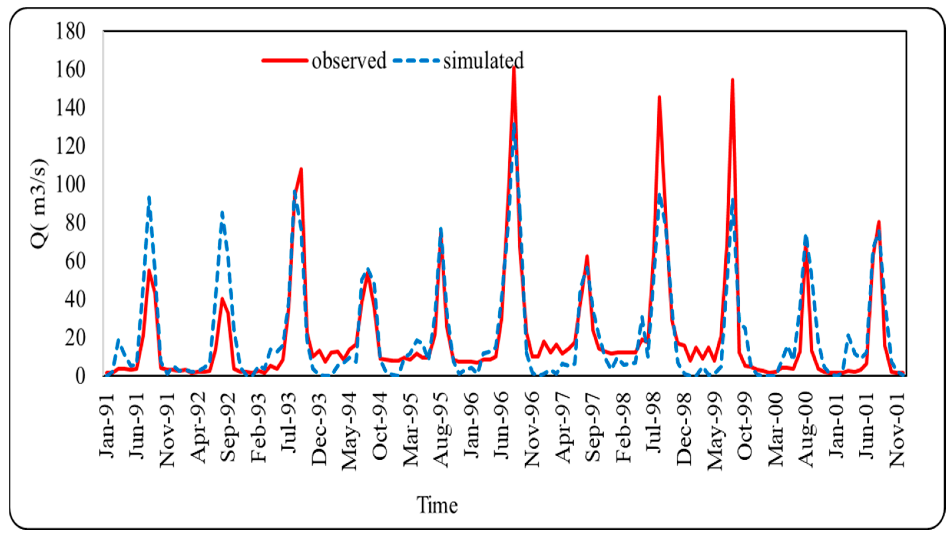
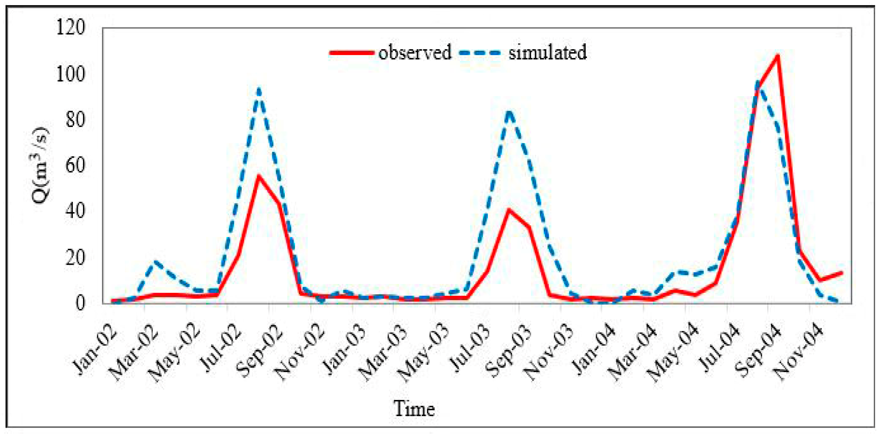
4.1. SWAT Mode Calibrated and Validated Result

The size of the data series, periodicity, the kind of basin, and the climate data can affect the efficiency of hydrologic model calibration [10]. To model the watershed water balance in terms of evapotranspiration, potential evapotranspiration, runoff, water yield, and lateral flow, the DEM, the soil map, the LU/C map, rainfall, and temperature were used to run the SWAT model [58] Hydrological model calibration in the study of the effect of climate change on the hydrological processes depends on the quality of observed meteorological data, the physical meaning of model parameters, the significance of parameters in the model, and the range of parameter values of the model [59].

In line with the research in [60,61,62,63] on the assessment of the climate change effect on the hydrology in the upper Awash basin using the SWAT model, the SWAT hydrological model seems to be the best model for simulating the hydrologic balance in the Akaki River basin. According to the hydrological network, the Akaki basin was divided into 29 sub-basins by the SWAT model with an average surface area of 1468 km². In this way, the surface area of the sub-catchment varies from 1.83 km² to 126.26 km². The sensitivity of 12 input parameters has been assessed using the Sequential Uncertainty Fitting (SUFI-2) algorithm of the computer program for calibration of SWAT model (SWAT-CUP) with global sensitivity methods. The ranking of the most sensitive calibrated parameters of the SWAT model is presented in

Table 1. Most sensitive parameters.

Parameter Code	Fitted Value	Min Value	Max Value	t-Stat	P	Rank
*CN2	0.07	−0.25	0.25	30.03	0.00	1
*ALPHA_BF	−0.11	0.04	0.69	13.25	0.00	2
*GW_DELAY	397.12	333.97	468.63	8.80	0.00	3
*GWQMN	0.55	0.24	1.03	8.43	0.00	4
*GW_REVAP	0.07	0.06	0.18	7.75	0.00	5
*ESCO	0.82	0.80	0.88	7.09	0.00	6
*CH_N2	0.13	0.04	0.16	5.76	0.01	7
*CH_K2	45.63	10.51	80.07	5.55	0.01	8
*ALPHA_BNK	0.35	0.19	0.40	4.43	0.02	9
*SOL_AWC	0.32	0.24	0.49	4.19	0.03	10
*SOL_K	0.79	0.01	1.41	3.13	0.05	11
*SOL_BD	0.24	0.9	0.92	2.40	0.09	12

Notes: *CN2 is the runoff curve number, *ALPHA_BF is the baseflow alpha factor in days, *GW_DELAY is the groundwater delay, *GWQMN is the threshold depth of water in the shallow aquifer required from return flow to occur in mm, *GW_REVAP is the groundwater “revap” coefficient, *ESCO is the soil evaporation compensation factor, *CH_N2 is Manning’s “n” for the main channel, *CH_K2 is the effective hydraulic conductivity in the main channel alluvium, *ALPHA_BNK is the baseflow alpha factor for bank storage, *SOL_AW is the available water capacity of the soil layer, *SOL_K is the saturated hydraulic content, and SOL_BD is the moist bulk density.

. As shown in Table 1 the sensitivity analysis result showed that the runoff curve number was the most sensitive parameter.

The SWAT model was calibrated and validated with observed streamflow from 1991 to 2004. Three-fourths were assigned for model calibration and one-fourth for model validation. Figure 5 and Figure 6 illustrate the graphical representation of simulated discharge during the calibration and validation phases. The monthly calibrated and validated results of the statistical value of R-square, the NSE, and PBIAS (%) were 0.78, 0.79, −1.6%, and 0.93, 0.91, and −16.2%, respectively. The P-factor and r-factor values were 0.8, 0.98, and 0.64 1.91 during calibration and validation, respectively. The overall performance of the SWAT model was good in the water balance simulation.

4.2. Change in Future Climate

4.2.1. Rainfall Projection under RCPs

A change in the average precipitation will affect the water balance elements of any catchment at any level. So, to determine the variation in water resources under climate change, it is imperative to identify the hotspot points for stakeholders and decision-makers in the catchment area. In our case, the local community uses Akaki River water resources for a different purpose, so knowing precipitation change is the most necessary point for water resources planning and management. It should be highlighted that the scenarios employed in this study could only estimate mean monthly and annual change in rainfall and temperature. The percentage change in the average precipitation in the Akaki catchment for the whole period of 60 years has been projected under RCP4.5 and RCP8.5 with two scenarios of each RCP. On an average month, under the RCP4.5 scenario, the projected rainfall indicates decreases in the rainy month of August by 0.6% and in October by 1.26% under RCP4.5 (2040s). And in the remaining months, it increases in the near scenarios. The projected rainfall increases up to 58.1% in May, 57.30% in February and 51.84% in December. In these three months, the precipitation will show a positive change from baseline by above 50%, and there might be flooding in the catchment under the RCP4.5 (2040s) scenario (

Table 2. Projected change rainfall under different climate scenarios (all values in percentages).

Month	RCP4.5 (2040s)	RCP4.5 (2060s)	RCP8.5 (2040s)	RCP8.5 (2060s)
January	45.42	−120.90	87.62	−88.77
February	57.30	73.54	59.89	68.48
March	45.48	24.55	24.30	43.02
April	27.11	46.32	27.27	35.96
May	58.10	52.89	41.44	34.77
June	10.60	21.77	−15.14	23.65
Jully	1.84	−4.13	−26.62	−9.40
August	−0.60	−3.74	2.02	2.48
September	21.66	5.65	27.38	29.03
October	−1.26	−73.32	−35.69	−81.06
November	24.44	46.11	40.28	55.52
December	51.84	−7.44	35.46	−10.25
Annual	14.96	8.39	4.13	10.89

). Annually, precipitation may rise over the catchment by 14.96% in the coming 30 years. According to rainfall projection, the Akaki River may face water scarcity in August and October, more in October in the nearest scenarios (in the 2040s) under RCP4.5.

Under RCP4.5 (in the 2060s), in January, July, August, October, and December, precipitation may decrease to 120.9%, 4.31%, 3.74%, 73.32%, and 7.44%, respectively. The watershed may face the highest shortage of rainfall in January and October. It is positively changed in the rest of the month in this scenario. The maximum change will occur in February by 73.53%, 52.89% in May, 46.32% in April, and 46.11% in November in this scenario. At the end of the coming 60 years, the rainfall projection indicated that the maximum and minimum negative change of more than 50% would be in January and October, with positive alterations in February and May. The average annual projected rainfall rose 8.39% in RCP4.5 (in the 2060s). More rises in annual projected change in rainfall may occur in the early scenario of RCP4.5 than in the latter scenario (Figure 7 and Table 2).

The precipitation changes under the RCP 8.5 scenario show a decrease of 35.69%, 26.62%, and 15.14% in October, July, and June under RCP 8.5 (in the 2040s). The rainfall shows an increment in magnitude in the rest of the months in RCP8.5 (2040s), as shown in Figure 7 and Table 2. The highest rainfall change will be seen in the river, 87.62% in January and 59.89% in February. The catchment and area surrounding the catchment may face flooding in these two months under RCP8.5 (in the 2040s). In the second scenario of RCP8.5, the greatest positive rainfall change of up to 68.48% may occur in February at the end of the coming 60 years. A decrement in rainfall of up to 88.77%, 81.06%, 10.25%, and 94.52% will happen in January, October, December, and July under RCP8.5 (in the 2060s). In the decreasing case of the projected precipitation on the monthly projection, in January, the maximum precipitation change would be in RCP4.5 (in the 2060s) than in RCP8.5 (in the 2060s), in December; and in October, the maximum change in RCP8.5 (in the 2060s), RCP4.5 (in the 2060s), RCP8.5 (in the 2040s) and RCP4.5 (in the 2040s) from large to slight projected rainfall. For the primary rainfall month in the catchment in July, there are RCP8.5 (in the 2040s), RCP8.5 (in the 2060s) and RCP4.5 (in the 2060s) scenarios from higher to lower projections. It increased over the Akaki catchment in the rest of the months except in August under RCP4.5 and June under RCP8.5 (in the 2040s). Annual projected rainfall rises by 4.13% in RCP8.5 (in the 2040s) and 10.89% in RCP8.5 (in the 2060s). Comparatively, in early scenarios, in the yearly rainfall projection case, the precipitation increases in RCP4.5 (the 2040s) by 14.96% and RCP8.5 (in the 2040s) by 4.13%, which is more prominent in the medium emission of RCP (CMIP5), but in the far scenarios, there is likely a greater increase in RCP8.5 (in the 2060s) by 10.39% than in RCP4.5 (in the 2060s) by 8.39%. As a conclusion on the precipitation projection, it would be a win–win change under early and far scenarios in the Akaki River. Overall, the modification of precipitation shows that rainfall increases more in RCP4.5 (in the 2040s) in the next 60 years under RCPs.

The numerical value of the projected rainfall changes from (−)0.6% to (+)57.3% under RCP4.5 (in the 2040s) and would vary from (−)120.90% to (+)73.54% under RCP4.5 (in the 2060s), (−)35.69% to (+)87.62% under RCP8.5 (in the 2040s) and (−)87.62% to (+)68.48% under RCP8.5 (in the 2060s). Similarly, the study in [64] has argued that the rainfall increases from 15% to 30% under three scenarios of RCP4.5 and 8.5. According to this research finding, precipitation would be decreased in October for both RCPs with differences in magnitude. In the medium emission of the CMIP5, the rainfall is expected to change from −120.9% to 58.10% on a mean monthly basis; and in the higher emission of the CMIP5, it will likely change from −88.70% to 87.62% on an average monthly basis.

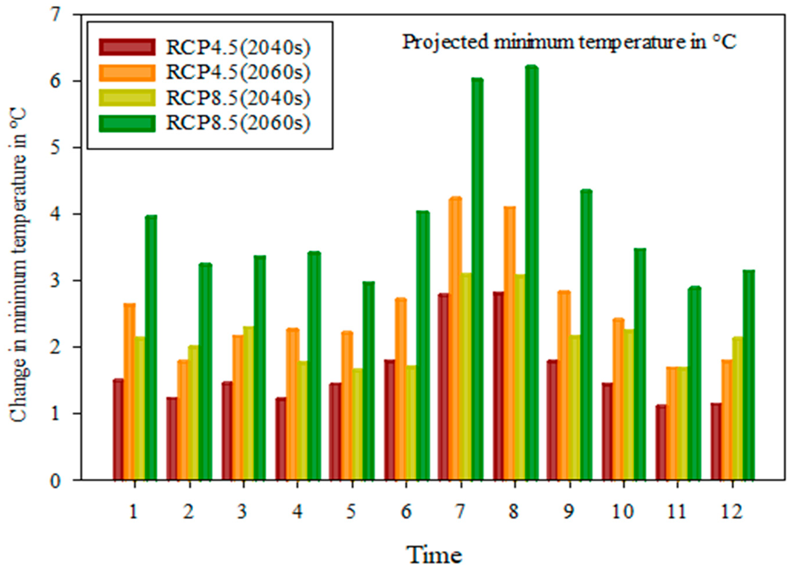
4.2.2. Change in Temperature under RCPs

Figure 8 and Figure 9 and

Table 3. Projected change temperature under different climate scenarios (unit = °C).

Month	RCP4.5 (2040s)		RCP4.5 (2060s)		RCP8.5 (2040s)		RCP8.5 (2060s)
	Tmin	Tmax	Tmin	Tmax	Tmin	Tmax	Tmin	Tmax
January	1.50	1.99	2.63	2.91	2.13	2.59	3.96	4.43
Februry	1.23	2.23	1.78	3.09	2.00	2.65	3.24	4.60
March	1.45	1.71	2.16	2.17	2.29	1.76	3.35	3.67
April	1.22	1.12	2.27	2.25	1.77	1.88	3.42	3.34
May	1.45	1.81	2.21	2.28	1.65	1.81	2.96	2.95
June	1.79	1.17	2.71	2.56	1.70	1.32	4.03	3.47
July	2.78	1.06	4.23	2.28	3.09	1.39	6.02	4.28
August	2.80	1.64	4.10	2.11	3.07	1.80	6.21	3.97
September	1.79	1.31	2.82	1.27	2.16	1.39	4.34	2.38
October	1.44	1.75	2.41	1.71	2.24	1.50	3.46	2.62
November	1.11	1.22	1.69	1.59	1.68	1.30	2.89	2.59
December	1.14	1.25	1.79	1.77	2.12	1.40	3.14	2.59
Annual	1.64	1.52	2.57	2.17	2.16	1.73	3.92	3.41

depict the projected maximum and minimum temperatures under different representative concentrations of the path of the CMIP5 scenarios. Future projections indicated that the maximum and minimum temperatures increase under RCPs in all the months and annually throughout the catchment. However, the magnitude of the change in each RCM would be higher in higher emission scenarios (RCP8.5) than in medium emission (RCP4.5). The overall projection indicated the change in minimum temperature will rise by 1.22 °C to 2.8 °C and 1.78 °C to 4.23 °C under RCP4.5 for the short and long projected periods. Similarly, the maximum temperature will increase from 1.06 °C to 2.22 °C, and from 2.17 °C to 3.09 °C under RCP4.5 (in the 2040s) and RCP4.5 (in the 2060s), respectively. The minimum temperature will increase by 1.65 °C to 3.09 °C and 2.96 °C to 6.02 °C under the first and second scenarios of high emission scenarios RCP8.5.

Similarly, the maximum temperature will increase from 1.32 °C to 2.65 °C and 2.95 °C to 4.6 °C under RCP8.5 (in the 2040s) and RCP8.5 (in the 2060s), respectively. The overall results of the investigation pointed out that the projected temperature shown under RCP4.5 would be cooler than RCP8.5. The change in projected temperature will increase monthly and annually under all scenarios (Table 3). In almost all months, there the maximum temperature change was lower in the first scenarios of RCP4.5 except in September and October, and on a mean annual basis (Figure 8). The projected maximum temperature result indicated that the most significant change may be seen in the Akaki catchment in the second scenario of RCP8.5, for both mean monthly and annual projections. Comparatively, monthly and yearly, higher maximum temperature change occurred across the catchment under RCP8.5 (in the 2060s). The maximum temperature projection developed under medium and higher emission scenarios over the river confirmed that the hydrological component of the catchment is probably more affected under higher emissions than under medium emissions.

Figure 9 and Table 3 show a lower change in the projected minimum temperature seen under RCP4.5 (in the 2040s) except in June and a higher change illustrated under RCP8.5 (in the 2060s) in monthly and annual. This result proved that higher emissions have a higher effect on the water resources in the catchment. The temperature change results found in this work agreed with previous research performed in different regions of Ethiopia by many researchers to analyze the impact of climate change on water resources and discharge, and they found that the temperature is likely to increase. However, the strength of change varies with the downscaling techniques and climate model types. The study in [65] confirmed the maximum temperature change projected to increase under RCP8.5 using five different GCMs in the Ilala watershed, Northern Ethiopia. In the upper Awash basin, Keleta watershed, Bekele et al. [61] found that in the mid-21st century, the projected mean minimum and maximum temperature is likely to rise from 1.8 to 1.6 °C under RCP4.5 and from 2.6 to 2.1 °C under RCP8.5. In comparison, at the end of the 21st century, it will rise from 2.4 to 2.0 °C under RCP 4.5 and 4.6 to 3.7 °C under RCP 8.5 of the CMIP5.

The study in [66] also showed that the average annual temperature will increase by 0.84 °C, 2.6 °C, and 4.1 °C for the periods RCP2.6, RCP4.5, and RCP8.5, respectively, over the Gumara watershed, upper Blue Nile basin. The study on the whole Awash River basin in [67] using the global and regional climate model further reported that the annual average temperature change in the 2050s and 2070s RCP4.5 simulation showed an increase of 0.48 °C–2.6 °C in maximum temperature. In the case of RCP8.5, the simulated maximum temperature increase reached 3.4 and 4.1 °C in the 2050s and 2070s, respectively. Furthermore, the study in [68] has confirmed the projected mean annual temperature expected to increase under RCP4.5 and RCP8.5 in the Mojo watershed, which supports the result found in the Akaki catchment. In general, the projection of maximum and minimum temperatures in the future are within the range projected by the IPCC and agree with that projected by other researchers. In the concept of projected temperature, we concluded that the temperature is expected to increase over the catchment, and the hydrological process, the hydrological cycle, and especially evaporation would be affected more. The maximum and minimum temperature rise less from the current in the catchment in the 2040s under RCP4.5 than in the 2040s under RCP8.5 and in the 2060s under RCP4.5 than in the 2060s under RCP8.5 in all months.

4.2.3. Projected Water Balance Response to Climate Change

Climate change affects water balance components within the catchment. The impact of climate variation on water has been extensively researched and published in several international reports and scholarly journals. Projected rainfall and temperature under RCP4.5 and 8.5 lead to an essential disproportion in the estimated water balance element of the Akaki catchment. The changes in amounts, time, and uneven distribution of rainfall in space directly affect water practices, and temperature also directly impacts the quality and quantity of water resources. Under this point, we discussed the change in evapotranspiration (E.T.), potential evapotranspiration (PET), surface runoff (SURQ), lateral flow (LAT_Q), and water yield (WYLD) due to climate change at the sub-catchment level, monthly and annual. The water balance components of the Akaki catchment were observed to shift due to the changes in temperature and rainfall from current conditions in the future.

4.3. Water Balance Change at the Sub-Basin Level

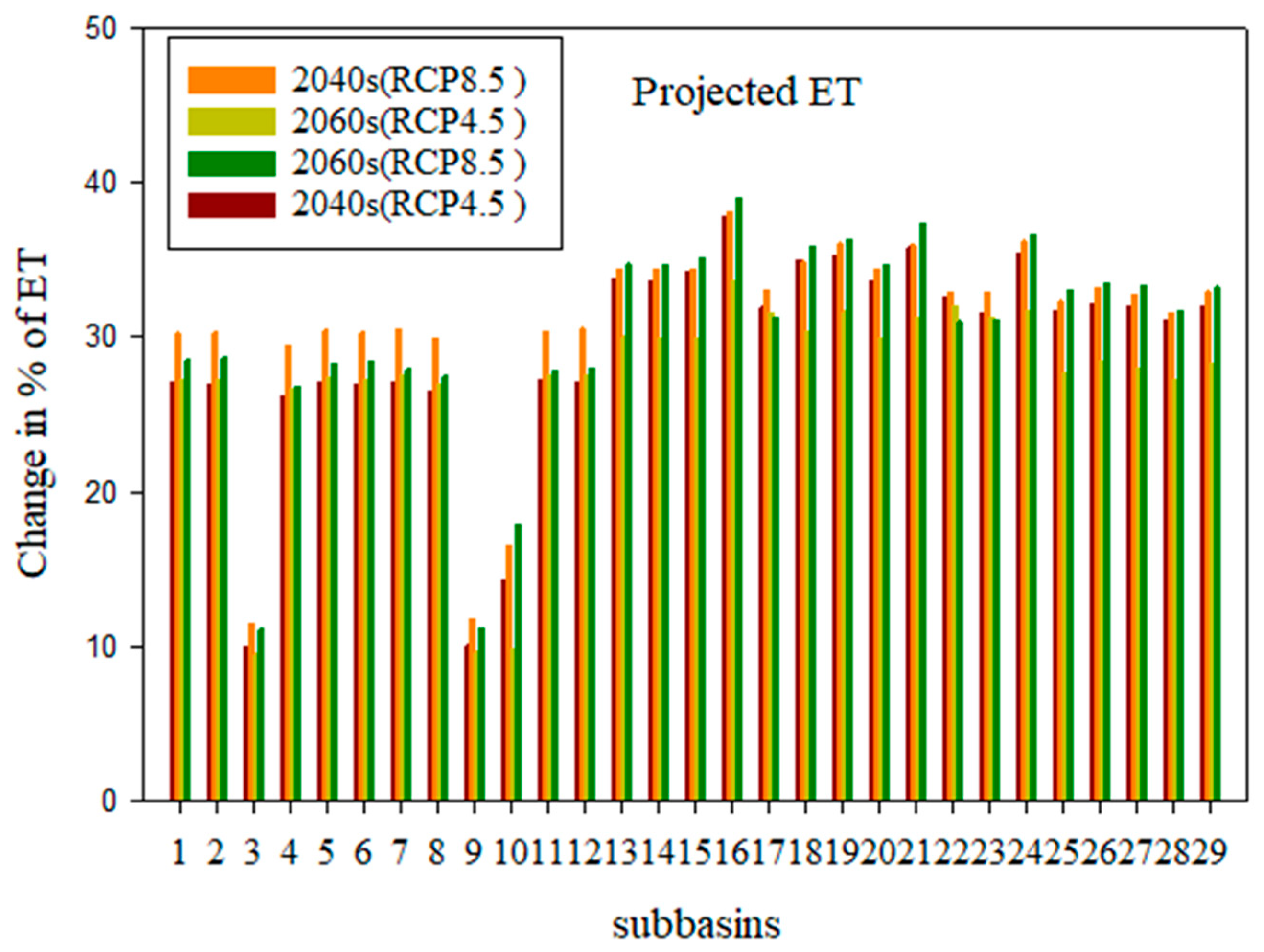
4.3.1. Change in Evapotranspiration at the Sub-Basin

Evapotranspiration is anticipated to grow in both the short- and long-term scenarios in each sub-basin of the Akaki watershed under both future scenarios (Figure 10). The hydrological process is significant in the water cycle and plays a critical role in the water budget in the area. It may not be affected by only precipitation and temperature changes; soil moisture, vegetation change, and other environmental aspects cause evapotranspiration change in the catchment. In this work, we focused more on the impact of the change in rainfall and temperature on the water balance elements. The overall projected evapotranspiration of the Akaki catchment increased from 29.51% to 31.09% in the coming first 30 years and 27.50% to 30.46% in the forthcoming second 30 years under RCP4.5 and RCP8.5 over all sub-basins, respectively.

Even though evapotranspiration rates are known to increase with higher temperatures, other factors, in addition to rising temperatures, also affect evapotranspiration. For instance, increasing humidity and higher CO₂ concentrations tend to reduce transpiration and frustrate the higher temperature effects on evapotranspiration. Global moisture will likely increase as the oceans and other water bodies warm and evaporate more water into the atmosphere, as carbon dioxide concentrations increase, leaf stomata partially close in response to keep the carbon dioxide concentration inside the stomata.

Consequently, although climate change is likely to increase air temperature, the effect of higher humidity and carbon dioxide concentration may partly counterbalance the temperature effect on evapotranspiration. Projected evapotranspiration in each sub-basin will be linked with the projected temperature and partly with precipitation across the watershed. The fluctuations in projected evapotranspiration are consistent with the temperature projections under the RCP scenarios. Compared to the linkage between rainfall and evapotranspiration, there is a more pronounced link between temperature and evapotranspiration. Low evapotranspiration is pronounced in sub-basins 3, 9, and 10. The overall change in evapotranspiration in all the sub-basins was equal to the overall annual projection. Future projected evapotranspiration in each sub-basin showed consistent change with temperature and inconsistent linkage with rainfall over the catchment.

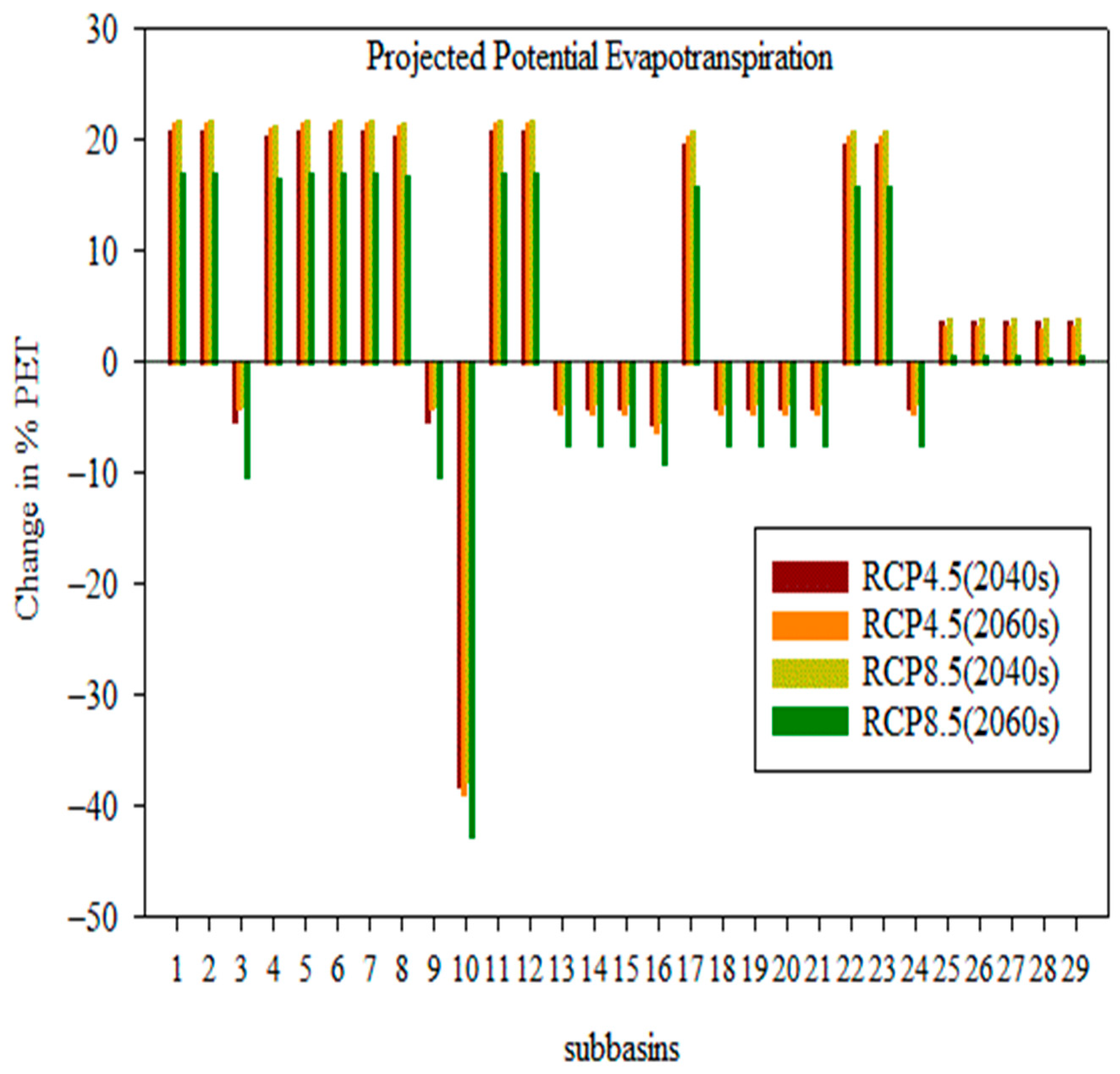
4.3.2. Change in Potential Evapotranspiration in the Sub-Basin

Potential evapotranspiration may decrease in sub-basins 3, 9, 10, 13 to 16, 18 to 21, and 24 under climate scenarios (Figure 11). The highest decline in potential evapotranspiration will be in sub-basin ten under each RCP, and a greater change in potential evapotranspiration will be seen under RCP8.5 (in the 2060s). In the rest of the sub-basin, PET would increase because of climate change in the watershed. Evaluating future potential evapotranspiration (PET) trends is imperative to find imaginable enduring indicators of climate change to formulate policy actions for managing water resource integration for single and multiple purposes. Sub-basin 10 will have a higher decrease compared with the other sub-basins. The highest PET increase and decrease will occur in the RCP8.5 (in the 2060s) scenarios. In addition to the air temperature, sunlight length, wind speed, and humidity also affect potential evaporation (ETo) in agronomic areas, plantations, and other areas. The latitude has a possible impact on evapotranspiration. The projected overall potential evapotranspiration of the catchment would be 6.4% under RCP4.5 (in the 2040s), 6.51% under RCP4.5 (in the 2060s), 7.14% under RCP8.5 (in the 2040s) and 2.8% under RCP8.5 (in the 2060s), which is the same annual projection over the catchment. The change in future potential evapotranspiration will not show a consistent connection with the projected temperature.

4.3.3. Change in Surface Runoff in the Sub-Basin

As shown in Figure 12 in each sub-basin, projected surface runoff may be decreased under both RCP scenarios and increased in sub-basin 3 by 2.14% in the 2040s under RCP4.5, sub-basin 9 by 0.97% (negligible change) under RCP4.5, and sub-basin 16 by 15.87% in the 2040s under RCP4.5; sub-basin 10 by 26.99% in the 2040s under RCP4.5, 8.87% in the 2060s under RCP4.5, 14.9% in the 2040s under RCP8.5 and 11.87% in the 2060s under RCP8.5. Surface runoff increased in sub-basin ten in all climate scenarios. According to the projection of overall runoff, climate change will increase the water problem in the catchment by decreasing runoff across the sub-basin. The surface runoff would likely decrease by 30.21%, 51.67%, 46.86%, and 42.47% under medium and higher emissions in the first 30 years and second 30 years, respectively.

4.3.4. Change in Water Yield in the Sub-Basin

Global and local climate change affects water yield. In line with this idea, the projected water yield in the Akaki catchment sub-basins decreased under both emissions except in sub-basins 10 and 16 (Figure 13). In sub-basin ten, the water yield increased by 53.82%, 41.67%, 43.07%, and 44.79% in the 2040s and 2060s of the RCP4.5 and RCP8.5 scenarios, respectively. In sub-basin sixteen, the water yield increased by 28.65%, 13.67%, 14.63%, and 18.43% in the 2040s and 2060s of the RCP4.5 and RCP8.5 scenarios, respectively. In sub-basin three, water yield increased by 11.24% in the 2040s under RCP4.5 and 12.61% in the 2060s under RCP8.5. In sub-basin nine, the projected water yield is rising by 11.21% in the 2040s under RCP4.5 and 12.68% in the 2060s under RCP8.5. The projected water yield indicated a higher decline in the 2060s under RCP4.5 and the 2040s under RCP8.5. It is likely to decrease by 31.1%, 54.11%, 55.73%, and 37.02% under the RCP4.5 and RCP8.5 scenarios.

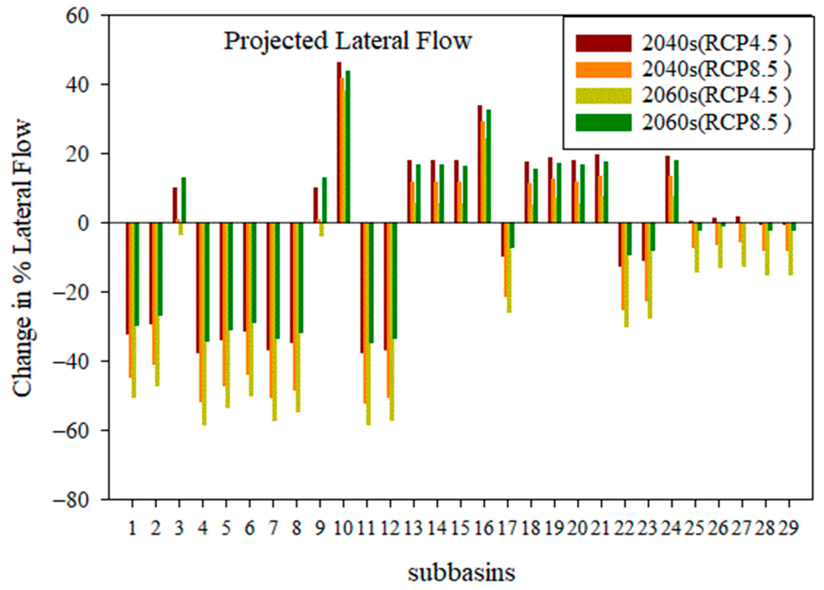
4.3.5. Change in Lateral Flow at the Sub-Basin

Climate change and variability alter the lateral flow of the basin. Under climate scenarios, a lateral flow deficit may be seen in the 2060s under RCP4.5 and the 2040s under RCP8.5. The maximum lateral flow rises for each scenario in sub-basin 10 (Figure 14). Due to variations in sub-basin natural environments, the increment and decrement of the lateral flow between medium and high emissions varies for each scenario.

4.4. Monthly and Annual Water Balance Change

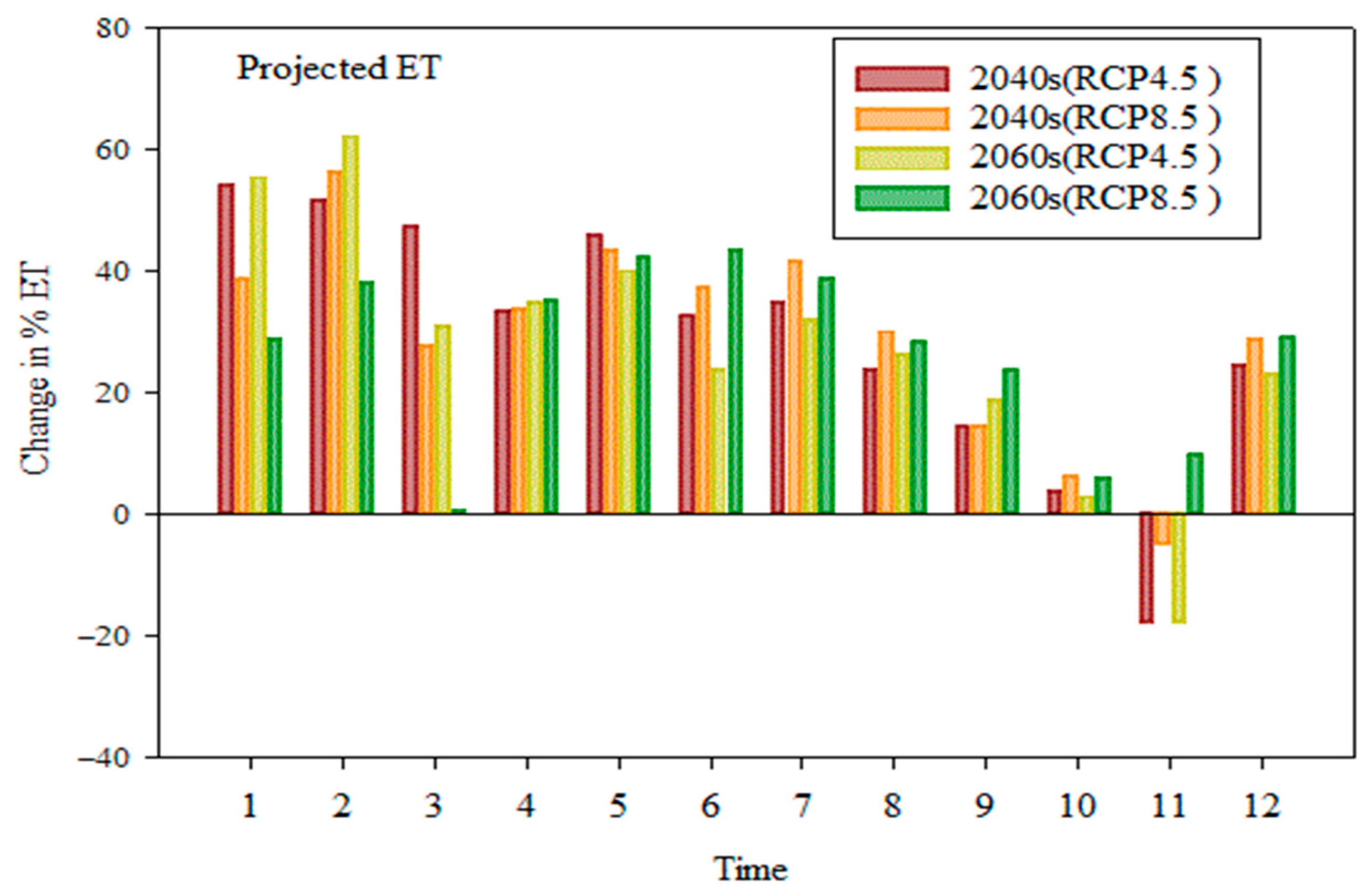
4.4.1. Change in Mean Monthly and Annual Evapotranspiration

Evapotranspiration (E.T.) is one of the most pertinent elements in the hydrologic cycle. It is acknowledged to be defined by an extensive diversity of local and periodic biophysical features exposed to climate change. On a mean monthly basis, evapotranspiration will increase in all months, except in November under RCP4.5 (in the 2040s, 2060s) and RCP8.5 (in the 2040s) (Figure 15). All scenarios suggested an annual increase in E.P. related to climate change. Under both RCPs, E.T. change indicates less than 100%. Evapotranspiration is the critical element of the water cycle that measures the quantity of water displaced. Evapotranspiration has a significant role in the process of hydrology and predicting the real change in evapotranspiration under different climate scenarios will provide a clue for hydrologists, agronomists, climatologists, and agricultural activities.

4.4.2. Change in Mean Monthly and Annual Potential Evapotranspiration

Hydrometeorology and other related sciences struggle with the realistic estimation of potential evapotranspiration (PET), which is an important aspect that needs to be considered in catchment water management and water resource distribution. It is likely to decrease by 1.32% in the 2060s under RCP4.5, increase from 2.07% to 16.25% (in the 2040s under RCP4.5), from −1.32% to 23.53% (in the 2060s under RCP4.5), 0.05% in the 2040s under RCP8.5, from −0.5% to 122.65% (in the 2040s under RCP8.5) and −6.79% to 17.33% (in the 2060s under RCP8.5). In the second scenario of RCP8.5, PET declined for six consecutive months, from January to June, and November is the seventh month. The mean yearly PET change is 6.41% (in the2040s under RCP4.5), 6.51% (in the 2040s under RCP4.5), 7.14% (in the 2040s under RCP8.5), and 2.8% (in the 2060s under RCP4.5). The largest percentage of the change in PET was identified under RCP8.5 (in the 2060s) for monthly and annual projections (Figure 16).

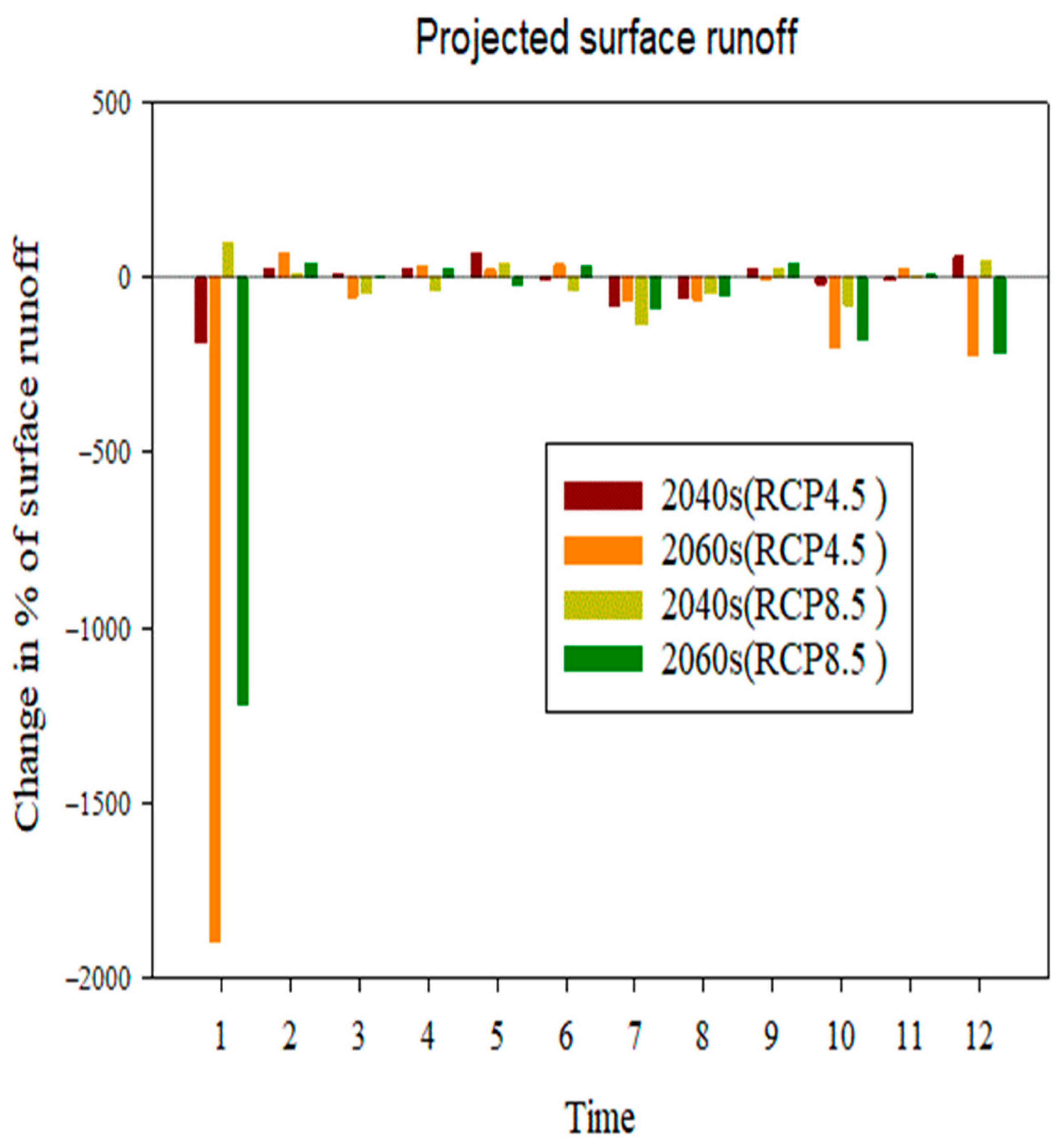
4.4.3. Change in Mean Monthly and Annual Surface Runoff

In the case of mean monthly runoff under the scenario two, the water balance component of the Akaki watershed, surface runoff decreases highly in January, followed by December, May, September, February, and November (Figure 17). In this scenario, the forecasted evapotranspiration showed only a positive change in November by 17.67% from the baseline and decreased each rest month and declined in annual percentage when compared with baseline. The yearly projected runoff under the RCP4.5 and RCP8.5 scenarios declined by 30.21%, 51.67%, 46.86%, and 42.47% in each scenario, respectively. This result agreed with the projected runoff in Hablehroud, Iran, in which annual runoff decreased by 11.44% under RCP4.5 and 13.13% under RCP8.5. In the coming 60 years, yearly surface runoff will be reduced (

Table 4. Projected annual change water balance components.

				Annual Change (%)
Scenarios		Time	LAT_Q	WYLD	SURQ	PET	ET
RCP4.5		2040s	−1.62	−31.10	−30.21	6.41	29.51
		2060s	−16.60	−54.11	−51.67	6.51	27.50
RCP8.5		2040s	−11.09	−55.73	−46.86	7.14	31.09
		2060s	−0.54	−37.02	−42.47	2.80	30.46

), but annual rainfall will increase under all scenarios.

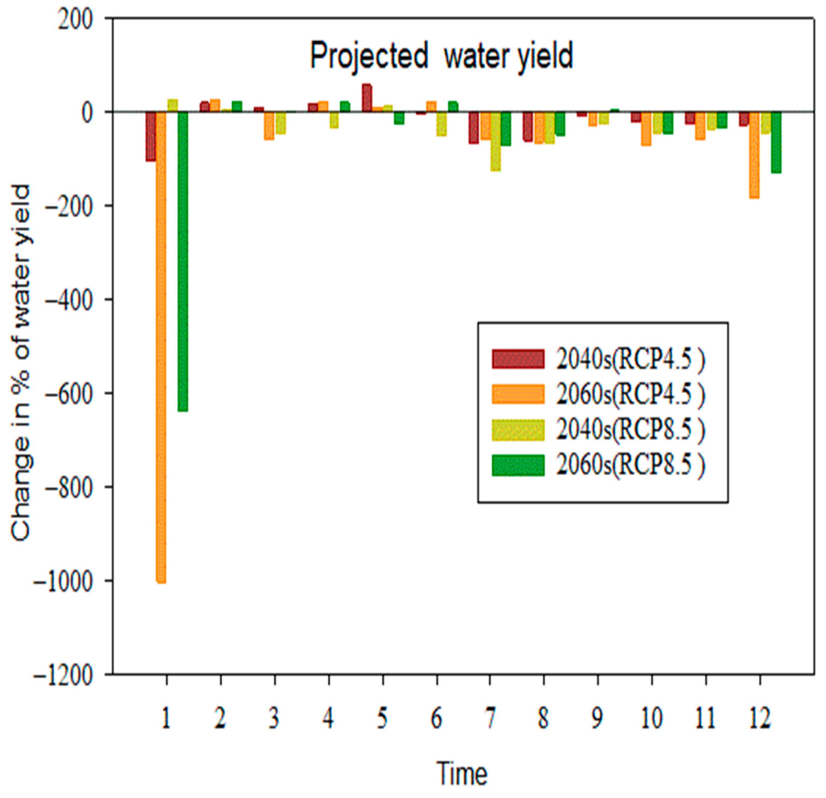
4.4.4. Change in Mean Monthly and Annual Water Yield

The catchment will see a positive change in water yield in February in both RCPs, April under RCP4.5 and in the 2060s (under RCP8.5), and June in the second of RCPs and September in the 2060s (under RCP8.5). Water yield also rises in January in the 2060s (under RCP8.5), and May under RCP4.5 and in the 2060s (under RCP8.5). However, water yield change under climate change is negative in the rest of the months, with a minor change in March in the 2040s (under RCP4.5) compared to the reference period. On an average annual basis for scenario one, the water balance element showed a negative change under the climate change in the Akaki catchment (Table 4). The projected water balance component change under climate change is shown in Figure 18.

4.4.5. Change in Mean Monthly and Annual Projected Lateral Flow

The negative and positive changes in the percentage of lateral flow are discussed in detail graphically in Figure 19. In all scenarios, projected lateral flow indicates that the catchment is expected to shift in water components in the coming 60 years. The indication of projected lateral flow change either positively or negatively under climate change can affect water use for energy production, irrigation use of water, domestic and non-domestic use of water, and daily social life standards.

On a mean monthly basis, lateral flow probably changes from −21.95% to 45.90% (in the 2040s under RCP4.5), −53.13% to 25.89% (in the 2060s under RCP4.5), −39.56% to 72.48% (in the 2060s under RCP8.5) and −54.62% to 38.70% (in the 2060s under RCP8.5). On an annual basis, it changes by −1.62% in the 2040s under RCP4.5, −11.09% in the 2060s under RCP4.5, −16.60% in the 2040s under RCP8.5 and −0.5% in the 2060s under RCP8.5 (Table 4)

The negative values indicate that the hydrological components will decrease over the catchment in 30 and 60 years. In Table 4, the positive values of the hydrological elements showed an excess amount of water for a specified year compared with the current hydrology of the catchment. Among water balance components, evapotranspiration and potential evapotranspiration showed consistent change under each climate scenario level, while lateral flow, water yield, and runoff showed inconsistent change from baseline at the sub-basin. Runoff from a catchment can be considered dependent on precipitation and evapotranspiration. The current trend of an increased amount of greenhouse gases in the atmosphere is expected to impact temperature and rainfall, which will probably alter the water balance in the catchment.

5. Conclusions and Recommendations

5.1. Conclusions

Many people are anticipated to experience water stress due to climate change in the Akaki River. The natural uncertainties in the predictability of the hydrologic cycle and the effects of water withdrawals on runoff make it challenging to establish apparent patterns from runoff data, making it difficult to predict the implications of climate change. The SWAT model has been effectively applied in the Akaki River to identify water balance component changes under current and future scenarios. The statistical downscale was applied to downscale future temperature and precipitation data for the Akaki basin from CMIP5 CORDEX-Africa for the two RCP scenarios, RCP4.5 and RCP8.5; the climate data for watershed hydrology modeling applied in extraction and bias correction of daily precipitation and temperature following the procedure implemented in [54] efficaciously captured the catchment temperature and rainfall. Bias correction was performed by using the distributing mapping method. Identifying sensitive parameters for the estimation of water balance components under climate change scenarios has provided insight into the hydrological processes of the basin and offered helpful information for water management at the catchment scale to solve the water-related problems of the local population. The current study focused on the changes in the temperature, precipitation, evapotranspiration, surface runoff, lateral runoff, and water yield of the Akaki catchment in the headwaters of the Awash basin under climate scenarios. The primary findings of this research are stated as follows:

✓

The CN2, ALPHA_BF, GW_DELAY, GWQMNm, GW_REVAP, and ESCO parameters were the most sensitive parameters among the 12 parameters proposed for calibration.

✓

The performance of the model was excellent during the validation period (2002–2004) and the calibration period (1991–2001) according to the criterion mentioned in [69].

✓

There is a change in minimum temperature by 1.22 °C to 4.23 °C, 1.68 °C to 6.21 °C and maximum temperature from 1.06 °C to 2.56 °C, 1.3 °C to 4.43 °C on the average monthly basis and 1.64 °C to 2.57 °C, 2.16 °C to 3.92 °C, 1.52 °C to 2.17 °C and 1.73 °C to 3.41 °C on a mean yearly basis under RCP4.5 and RCP8.5, respectively, and the change in rainfall is expected by −120.90% to 58.10%, −88.72% to 87.62% on a monthly basis and from 14.96% to 8.39% and 4.13% to 10.89% on a yearly basis in the Akaki catchment.

✓

Compared to the baseline state, the effects of climate change on surface runoff range from −30.21% to −50.67%, potential evapotranspiration changes from 2.8% to 7.14%, evapotranspiration rises from 27.50% to 31.09%,l flow changes from −16.6% to –0.54%, and water yield changes from −31.1% to −55.73%.

✓

Water yield, lateral flow, and surface runoff showed remarkable negative and positive changes under both scenarios, but evapotranspiration and potential evapotranspiration showed positive increments in RCP at the sub-basin level.

According to this study, climate change will most likely impact the water balance component by the end of the 30 and 60 years. This study supports and raises awareness of the potential future impacts of climate change on water balance and drought in this river basin. The results show that water availability will be significantly affected in the medium and long term. Therefore, policy makers of the catchment need to develop climate change adaptation measures to ensure environmental and economic sustainability in the area.

5.2. Recommendations

Depending on the research findings, the authors recommended that future researchers address strategic planning for adaptation mechanisms to reduce negative and positive climate change effects in the catchment. The majority of work performed here was to clarify the impact of climate change on water balance components under different climate scenarios; it is necessary to apply land use/cover scenarios to obtain sound results to give more tangible information about future water resource challenges and ensure proper planning and management. A single hydrological model, the SWAT model, was applied to simulate hydrological components. Therefore, using different hydrological models is recommended in the future to obtain more accurate information on hydrological component responses to climate change. Multisite gauged calibration and validation of streamflow can be applied to improve hydrological model performance and increase the confidence of the modelers. The efficiency of a single climate model output in assessing water balance components may not be good enough. Multiclimate models can be applied to reduce the uncertainty of a single climate model and to ensure the degree of water balance response to climate change. A single bias correction and reproduction of precipitation and temperature may not be enough. Consequently, using different bias correction techniques is better to increase the connection between observed and climate data.

References

1. Zerga, B.; Mengesha, G.G. Climate Change in Ethiopia Variability, Impact, Mitigation, and Adaptation Journal of Social Science and Humanities Research. Int. J. Sci. Humanit. Res. 2016, 2, 66–84. [Google Scholar]
2. Abesh, B.F.; Jin, L.; Hubbart, J.A. Predicting Climate Change Impacts on Water Balance Components of a Mountainous Watershed in the Northeastern USA. Water 2022, 14, 3349. [Google Scholar] [CrossRef]
3. Ayele, H.S.; Li, M.H.; Tung, C.P.; Liu, T.M. Impact of climate change on runoff in the Gilgel Abbay watershed, the upper Blue Nile Basin, Ethiopia. Water 2016, 8, 380. [Google Scholar] [CrossRef]
4. Soltani, F.; Javadi, S.; Roozbahani, A.; Massah Bavani, A.R.; Golmohammadi, G.; Berndtsson, R.; Ghordoyee Milan, S.; Maghsoudi, R. Assessing Climate Change Impact on Water Balance Components Using Integrated Groundwater–Surface Water Models (Case Study: Shazand Plain, Iran). Water 2023, 15, 813. [Google Scholar] [CrossRef]
5. Balcha, S.K.; Awass, A.A.; Hulluka, T.A.; Bantider, A.; Ayele, G.T. Assessment of future climate change impact on water balance components in Central Rift Valley Lakes Basin, Ethiopia. J. Water Clim. Chang. 2023, 14, 175–199. [Google Scholar] [CrossRef]
6. Githui, F.; Gitau, W.; Mutua, F.; Bauwens, W. Climate change impact on SWAT simulated streamflow in western Kenya. Int. J. Climatol. 2009, 29, 1823–1834. [Google Scholar] [CrossRef]
7. Unnisa, Z.; Govind, A.; Lasserre, B.; Marchetti, M. Water Balance Trends along Climatic Variations in the Mediterranean Basin over the Past Decades. Water 2023, 15, 1889. [Google Scholar] [CrossRef]
8. Stathi, E.; Kastridis, A.; Myronidis, D. Analysis of Hydrometeorological Characteristics and Water Demand in Semi-Arid Mediterranean Catchments under Water Deficit Conditions. Climate 2023, 11, 137. [Google Scholar] [CrossRef]
9. Todaro, V.; D’Oria, M.; Secci, D.; Zanini, A.; Tanda, M.G. Climate Change over the Mediterranean Region: Local Temperature and Precipitation Variations at Five Pilot Sites. Water 2022, 14, 2499. [Google Scholar] [CrossRef]
10. Sahana, V.; Timbadiya, P.V. Spatiotemporal Variation of Water Availability under Changing Climate: Case Study of the Upper Girna Basin, India. J. Hydrol. Eng. 2020, 25, 05020004. [Google Scholar] [CrossRef]
11. Adhikari, U.; Nejadhashemi, A.P. Impacts of Climate Change on Water Resources in Malawi. J. Hydrol. Eng. 2016, 21, 05016026. [Google Scholar] [CrossRef]
12. Adhikari, U.; Nejadhashemi, A.P.; Woznicki, S.A. Climate change and eastern Africa: A review of impact on major crops. Food Energy Secur. 2015, 4, 110–132. [Google Scholar] [CrossRef]
13. Mehan, S.; Kannan, N.; Neupane, R.P.; McDaniel, R.; Kumar, S. Climate change impacts on the hydrological processes of a small agricultural watershed. Climate 2016, 4, 56. [Google Scholar] [CrossRef]
14. Negewo, T.F.; Sarma, A.K. Estimation of Water Yield under Baseline and Future Climate Change Scenarios in Genale Watershed, Genale Dawa River Basin, Ethiopia, Using SWAT Model. J. Hydrol. Eng. 2021, 26, 05020051. [Google Scholar] [CrossRef]
15. Reshmidevi, T.V.; Nagesh Kumar, D.; Mehrotra, R.; Sharma, A. Estimation of the climate change impact on a catchment water balance using an ensemble of GCMs. J. Hydrol. 2018, 556, 1192–1204. [Google Scholar] [CrossRef]
16. Němečková, S.; Slámová, R.; Šípek, V. Climate change impact assessment on various components of the hydrological regime of the Malše river basin. J. Hydrol. Hydromech. 2011, 59, 131–143. [Google Scholar] [CrossRef]
17. Nasonova, O.N.; Gusev, Y.M.; Kovalev, E. Climate Change Impact on Water Balance Components in Arctic River Basins. Geogr. Environ. Sustain. 2022, 15, 148–157. [Google Scholar] [CrossRef]
18. Eder, G.; Fuchs, M.; Nachtnebel, H.P.; Loibl, W. Semi-distributed modelling of the monthly water balance in an alpine catchment. Hydrol. Process. 2005, 19, 2339–2360. [Google Scholar] [CrossRef]
19. Gao, X.; Peng, S.; Wang, W.; Xu, J.; Yang, S. Spatial and temporal distribution characteristics of reference evapotranspiration trends in Karst area: A case study in Guizhou Province, China. Meteorol. Atmos. Phys. 2016, 128, 677–688. [Google Scholar] [CrossRef]
20. Stergiadi, M.; Di Marco, N.; Avesani, D.; Righetti, M.; Borga, M. Impact of geology on seasonal hydrological predictability in alpine regions by a sensitivity analysis framework. Water 2020, 12, 2255. [Google Scholar] [CrossRef]
21. Stone, M.C.; Hotchkiss, R.H.; Stone, A.B. Climate change impacts on missouri river basin water yields: The influence of temporal scales. In World Water Congress 2005: Impacts of Global Climate Change—Proceedings of the 2005 World Water and Environmental Resources Congress; ASCE: Reston, VA, USA, 2005; p. 461. [Google Scholar] [CrossRef]
22. Nie, T.; Yuan, R.; Liao, S.; Zhang, Z.; Gong, Z.; Zhao, X.; Chen, P.; Li, T.; Lin, Y.; Du, C.; et al. Characteristics of Potential Evapotranspiration Changes and Its Climatic Causes in Heilongjiang Province from 1960 to 2019. Agriculture 2022, 12, 2017. [Google Scholar] [CrossRef]
23. Liu, J.; Xue, B.; Yinglan, A.; Sun, W.; Guo, Q. Water balance changes in response to climate change in the upper Hailar River Basin, China. Hydrology Research 2020, 51, 1023–1035. [Google Scholar] [CrossRef]
24. Zhang, B.; Shrestha, N.K.; Daggupati, P.; Rudra, R.; Shukla, R.; Kaur, B.; Hou, J. Quantifying the impacts of climate change on streamflow dynamics of two major rivers of the Northern Lake Erie basin in Canada. Sustainability 2018, 10, 2897. [Google Scholar] [CrossRef]
25. Yin, Z.; Feng, Q.; Zou, S.; Yang, L. Assessing variation in water balance components in mountainous Inland River Basin experiencing climate change. Water 2016, 8, 472. [Google Scholar] [CrossRef]
26. Uniyal, B.; Jha, M.K.; Verma, A.K. Assessing Climate Change Impact on Water Balance Components of a River Basin Using SWAT Model. Water Resour. Manag. 2015, 29, 4767–4785. [Google Scholar] [CrossRef]
27. Elias, G. Impact of climate change on Lake Chamo Water Balance, Ethiopia. Int. J. Water Resour. Environ. Eng. 2017, 9, 86–95. [Google Scholar] [CrossRef]
28. Taye, M.T.; Dyer, E.; Hirpa, F.A.; Charles, K. Climate change impact on water resources in the Awash basin, Ethiopia. Water 2018, 10, 1560. [Google Scholar] [CrossRef]
29. Chelkeba Tumsa, B. Statistical and SWAT Model-Based Performance Evaluation of RCMs in Modeling Streamflow and Sediment Yield at Upper Awash Sub-Basin, Ethiopia. Appl. Environ. Soil Sci. 2022, 2022, 9193516. [Google Scholar] [CrossRef]
30. Jilo, N.B.; Gebremariam, B.; Harka, A.E.; Woldemariam, G.W.; Behulu, F. Evaluation of the impacts of climate change on sediment yield from the Logiya Watershed, Lower Awash Basin, Ethiopia. Hydrology 2019, 6, 81. [Google Scholar] [CrossRef]
31. Tessema, N.; Kebede, A.; Yadeta, D. Modelling the effects of climate change on streamflow using climate and hydrological models: The case of the Kesem sub-basin of the Awash River basin, Ethiopia. Int. J. River Basin Manag. 2021, 19, 469–480. [Google Scholar] [CrossRef]
32. Endris, H.S.; Omondi, P.; Jain, S.; Lennard, C.; Hewitson, B.; Chang’a, L.; Awange, J.L.; Dosio, A.; Ketiem, P.; Nikulin, G.; et al. Assessment of the performance of CORDEX regional climate models in simulating East African rainfall. J. Clim. 2013, 26, 8453–8475. [Google Scholar] [CrossRef]
33. Chala Daba, G.; Leta, G. Climate Change Induced Temperature Prediction and Bias Correction in Finchaa Watershed. Am. J. Agric. 2018, 18, 324–337. Available online: https://www.idosi.org/aejaes/jaes18(6)18/4.pdf (accessed on 20 October 2023).
34. Legese Jima, W.; Korecha, D.; Tur, K. Impact of Climate Change on Seasonal Rainfall Patterns over Bale Highlands, Southeastern Ethiopia. Int. J. Environ. Chem. 2019, 3, 84. [Google Scholar] [CrossRef]
35. Tangang, F.; Chung, J.X.; Juneng, L.; Supari; Salimun, E.; Ngai, S.T.; Jamaluddin, A.F.; Mohd, M.S.F.; Cruz, F.; Narisma, G.; et al. Projected future changes in rainfall in Southeast Asia based on CORDEX–SEA multi-model simulations. Clim. Dyn. 2020, 55, 1247–1267. [Google Scholar] [CrossRef]
36. Ashaley, J.; Anornu, G.K.; Awotwi, A.; Gyamfi, C.; Anim-Gyampo, M. Performance evaluation of Africa CORDEX regional climate models: Case of Kpong irrigation scheme, Ghana. Spatial Information Research 2020, 28, 735–753. [Google Scholar] [CrossRef]
37. Dibaba, W.T.; Miegel, K.; Demissie, T.A. Evaluation of the CORDEX regional climate models performance in simulating climate conditions of two catchments in Upper Blue Nile Basin. Dyn. Atmos. Ocean. 2019, 87, 101104. [Google Scholar] [CrossRef]
38. Karam, S.; Zango, B.S.; Seidou, O.; Perera, D.; Nagabhatla, N.; Tshimanga, R.M. Impacts of Climate Change on Hydrological Regimes in the Congo River Basin. Sustainability 2023, 15, 6066. [Google Scholar] [CrossRef]
39. Abbas, N.; Wasimi, S.A.; Al-Ansari, N. Impacts of Climate Change on Water Resources in Diyala River Basin, Iraq. J. Civ. Eng. Archit. 2016, 10, 1059–1074. [Google Scholar] [CrossRef]
40. Nasser Hilo, A.; Saeed, F.H.; Al-Ansari, N. Impact of Climate Change on Water Resources of Dokan Dam Watershed. Engineering 2019, 11, 464–474. [Google Scholar] [CrossRef]
41. Leta, O.T.; El-Kadi, A.I.; Dulai, H.; Ghazal, K.A. Assessment of climate change impacts on water balance components of Heeia watershed in Hawaii. J. Hydrol. Reg. Stud. 2016, 8, 182–197. [Google Scholar] [CrossRef]
42. Hargreaves, G.H.; Samani, Z.A. Reference Crop Evapotranspiration from Temperature. Appl. Eng. Agric. 1985, 1, 96–99. [Google Scholar] [CrossRef]
43. Neitsch, S.; Arnold, J.; Kiniry, J.; Williams, J. Soil & Water Assessment Tool Theoretical Documentation Version 2009; Texas Water Resources Institute: College Station, TX, USA, 2011; pp. 1–647. Available online: https://swat.tamu.edu/docs/ (accessed on 20 October 2023).
44. Abbaspour, K.C.; Vaghefi, S.A.; Srinivasan, R. A guideline for successful calibration and uncertainty analysis for soil and water assessment: A review of papers from the 2016 international SWAT conference. Water 2017, 10, 6. [Google Scholar] [CrossRef]
45. Serur, A.B. Performance evaluation of hydrological model in simulating streamflow and water balance analysis: Spatiotemporal calibration and validation in the upper Awash sub-basin in Ethiopia. Sustain. Water Resour. Manag. 2023, 9, 48. [Google Scholar] [CrossRef]
46. Arnold, J.G.; Moriasi, D.N.; Gassman, P.W.; Abbaspour, K.C.; White, M.J. SWAT: Model use, calibration, and validation. Biol. Syst. Eng. 2012, 55, 1491–1508. [Google Scholar]
47. Ashraf Vaghefi, S.; Mousavi, S.J.; Abbaspour, K.C.; Srinivasan, R.; Arnold, J.R. Integration of hydrologic and water allocation models in basin-scale water resources management considering crop pattern and climate change: Karkheh River Basin in Iran. Reg. Environ. Change 2013, 15, 475–484. [Google Scholar] [CrossRef]
48. Sao, D.; Kato, T.; Tu, L.H.; Thouk, P.; Fitriyah, A.; Oeurng, C. Evaluation of different objective functions used in the sufi-2 calibration process of swat-cup on water balance analysis: A case study of the pursat river basin, cambodia. Water 2020, 12, 2901. [Google Scholar] [CrossRef]
49. Almeida, R.A.; Pereira, S.B.; Pinto, D.B.F. Calibration and validation of the SWAT hydrological model for the Mucuri river basin. Eng. Agric. 2018, 38, 55–63. [Google Scholar] [CrossRef]
50. Jajarmizadeh, M.; Sidek, L.M.; Harun, S.; Salarpour, M. Optimal Calibration and Uncertainty Analysis of SWAT for an Arid Climate. Air Soil Water Res. 2017, 10, 1178622117731792. [Google Scholar] [CrossRef]
51. Nash, J.E.; Sutcliffe, J. V River Flow Forecasting through Conceptual Models—Part I—A Discussion of Principles. J. Hydrol. 1970, 10, 282–290. [Google Scholar] [CrossRef]
52. Teutschbein, C.; Seibert, J. Is bias correction of regional climate model (RCM) simulations possible for non-stationary conditions. Hydrol. Earth Syst. Sci. 2013, 17, 5061–5077. [Google Scholar] [CrossRef]
53. Kim, K.B.; Kwon, H.H.; Han, D. Intercomparison of joint bias correction methods for precipitation and flow from a hydrological perspective. J. Hydrol. 2022, 604, 127261. [Google Scholar] [CrossRef]
54. Rathjens, H.; Bieger, K.; Srinivasan, R.; Arnold, J.G. CMhyd User Manual Documentation for Preparing Simulated Climate Change Data for Hydrologic Impact Studies; SWAT: Huston, TX, USA, 2016. [Google Scholar]
55. Brighenti, T.M.; Gassman, P.W.; Gutowski, W.J.; Thompson, J.R. Assessing the Influence of a Bias Correction Method on Future Climate Scenarios Using SWAT as an Impact Model Indicator. Water 2023, 15, 750. [Google Scholar] [CrossRef]
56. Hassan, S.; Masood, M.U.; Haider, S.; Anjum, M.N.; Hussain, F.; Ding, Y.; Shangguan, D.; Rashid, M.; Nadeem, M.U. Investigating the Effects of Climate and Land Use Changes on Rawal Dam Reservoir Operations and Hydrological Behavior. Water 2023, 15, 2246. [Google Scholar] [CrossRef]
57. Tilahun, Z.A.; Bizuneh, Y.K.; Mekonnen, A.G. The impacts of climate change on hydrological processes of Gilgel Gibe catchment, southwest Ethiopia. PLoS ONE 2023, 18, e0287314. [Google Scholar] [CrossRef]
58. Arnold, J.G.; Kiniry, J.R.; Srinivasan, R.; Williams, J.R.; Haney, E.B.; Neitsch, S.L. Swat-Io-Documentation-2012.Pdf. 2012. [Google Scholar]
59. Majone, B.; Avesani, D.; Zulian, P.; Fiori, A.; Bellin, A. Analysis of high streamflow extremes in climate change studies: How do we calibrate hydrological models? Hydrol. Earth Syst. Sci. 2022, 26, 3863–3883. [Google Scholar] [CrossRef]
60. Chelkeba, B.; Feyessa, F.F.; Dibaba, W.T. Climate change in the upper Awash subbasin and its possible impacts on the stream flow, Oromiyaa, Ethiopia. Water Sci. 2023, 37, 179–197. [Google Scholar] [CrossRef]
61. Bekele, D.; Alamirew, T.; Kebede, A.; Zeleke, G.; Melesse, A.M. Modeling Climate Change Impact on the Hydrology of Keleta Watershed in the Awash River Basin, Ethiopia. Environ. Model. Assess. 2019, 24, 95–107. [Google Scholar] [CrossRef]
62. Alemu, M.G.; Wubneh, M.A.; Worku, T.A. Impact of climate change on hydrological response of Mojo river catchment, Awash river basin, Ethiopia. Geocarto Int. 2022, 2152497. [Google Scholar] [CrossRef]
63. Emiru, N.C.; Recha, J.W.; Thompson, J.R.; Belay, A.; Aynekulu, E.; Manyevere, A.; Demissie, T.D.; Osano, P.M.; Hussein, J.; Molla, M.B.; et al. Impact of Climate Change on the Hydrology of the Upper Awash River Basin, Ethiopia. Hydrology 2022, 9, 3. [Google Scholar] [CrossRef]
64. Ashu, A.B.; Lee, S. Il Assessing climate change effects on water balance in a monsoon watershed. Water 2020, 12, 2564. [Google Scholar] [CrossRef]
65. Chaemiso, S.E.; Abebe, A.; Pingale, S.M. Assessment of the impact of climate change on surface hydrological processes using SWAT: A case study of Omo-Gibe river basin, Ethiopia. Model. Earth Syst. Environ. 2016, 2, 1–15. [Google Scholar] [CrossRef]
66. Chakilu, G.G.; Sándor, S.; Zoltán, T. Change in stream flow of gumara watershed, upper blue nile basin, ethiopia under representative concentration pathway climate change scenarios. Water 2020, 12, 3046. [Google Scholar] [CrossRef]
67. Tadese, M.T.; Kumar, L.; Koech, R. Climate change projections in the Awash River Basin of Ethiopia using Global and Regional Climate Models. Int. J. Climatol. 2020, 40, 3649–3666. [Google Scholar] [CrossRef]
68. Gurara, M.A.; Jilo, N.B.; Tolche, A.D.; Kassa, A.K. Climate change projection using the statistical downscaling model in Modjo watershed, upper Awash River Basin, Ethiopia. Int. J. Environ. Sci. Technol. 2022, 19, 8885–8898. [Google Scholar] [CrossRef]
69. Moriasi, D.N.; Arnold, J.G.; Van Liew, M.W.; Bingner, R.L.; Harmel, R.D.; Veith, T.L. Model evaluation guidelines for systematic quantification of accuracy in watershed simulations. Trans. ASABE 2007, 50, 885–900. [Google Scholar] [CrossRef]
Figure 1. Map of the study area.
Water 16 00054 g001
Figure 2. Land use/cover.
Water 16 00054 g002
Figure 3. Soil type.
Water 16 00054 g003
Figure 4. Flowchart framework of study.
Water 16 00054 g004
Figure 5. Observed versus simulated for calibration from 1991 to 2001.
Water 16 00054 g005
Figure 6. Observed versus simulated for validation from 2002 to 2004.
Water 16 00054 g006
Figure 7. Projected rainfall under different climate scenarios.
Water 16 00054 g007
Figure 8. Projected monthly maximum temperature under different climate scenarios.
Water 16 00054 g008
Figure 9. Projected monthly minimum temperature under different climate scenarios.
Water 16 00054 g009
Figure 10. Projected evapotranspiration under different climate scenarios.
Water 16 00054 g010
Figure 11. Projected potential evapotranspiration under different climate scenarios.
Water 16 00054 g011
Figure 12. Projected surface runoff under different climate scenarios.
Water 16 00054 g012
Figure 13. Projected water yield under different climate scenarios.
Water 16 00054 g013
Figure 14. Projected lateral flow under different climate scenarios.
Water 16 00054 g014
Figure 15. Projected monthly evapotranspiration under different climate scenarios.
Water 16 00054 g015
Figure 16. Projected monthly potential evapotranspiration under climate scenarios.
Water 16 00054 g016
Figure 17. Projected monthly surface runoff under different climate scenarios.
Water 16 00054 g017
Figure 18. Projected monthly water yield under different climate scenarios.
Water 16 00054 g018
Figure 19. Projected monthly lateral flow under different climate scenarios.
Water 16 00054 g019