Optimization Design of the Elbow Inlet Channel of a Pipeline Pump Based on the SCSO-BP Neural Network

Abstract

A vertical pipeline pump is a type of single-stage, single-suction centrifugal pump with a curved elbow input. The inhomogeneous flow of the impeller inlet coexists with the unique elbow inlet channel, making it simple to generate the inlet vortical secondary flow. This paper aimed to optimize elbow inlet channel performance using a backpropagation (BP) neural network enhanced by the Sand Cat Swarm algorithm. The elbow flow channel’s midline and cross section shapes were fitted with a spline curve, and the parametric model of the curve was then constructed. Nine initial variables were filtered down to four optimization variables using the partial factor two-level (P2) and Plackett-Burman (P-B) experimental designs and multivariate analysis of variance. The sample space was generated by 50 groups of experiment samples, and the Sand Cat Swarm algorithm to optimize the BP (SCSO-BP) neural network and the approximation model of four variables were built. A genetic algorithm (GA) was applied to determine the optimal parameters among the approximate models in the sample space, and the ideal parameter combination of the elbow inlet channel was achieved. The findings demonstrated a strong agreement between the experimental and numerical simulation results. With reduced error fluctuation in inaccuracy and a more consistent fluctuation range, the approximate prediction model based on the optimized Sand Cat Swarm algorithm performed better. The optimized inlet model minimized the impact loss on the inlet wall, improved the velocity distribution uniformity of the inlet impeller, increased the pump efficiency by about 5% and the head by about 7.48% near the design flow, and broadened the efficient region of the pump.

1. Introduction

The optimized design of elbow-shaped flow passages in vertical pipeline pumps has remained a crucial issue in pipeline engineering [1]. Optimizing the elbow-shaped inlet can enhance the fluid flow characteristics into the impeller, reduce energy losses and hydraulic impact losses, and improve the performance and efficiency of pipeline systems.

Past studies have explored various optimization methods to address energy losses and uneven flow problems associated with elbow-shaped inlets. These methods include designs based on fluid mechanics simulations, empirical formulas, fluid mechanics principles, and multi-objective optimization. Research by Shi Wei [2] discovered that designing the elbow-shaped inlet cross-section according to linear gradient principles significantly improved the uniformity of outlet flow velocity distribution. Zhang Chi [3], through numerical simulation studies, found that appropriately increasing the radius of curvature (R) of the outer circle in the rear bend of the elbow-shaped channel significantly reduced hydraulic losses. AV Semenova [4] proposed a multi-objective optimization method to design the elbow tailpipe, but the excessive parameters led to inconclusive optimization results. While these studies presented effective design solutions, most focused on fluid numerical simulations, exhibiting limitations such as high computational complexity, time consumption, and limitations in optimizing multiple parameters or achieving precise design outcomes within limited optimization space.

In recent years, employing swarm intelligence algorithms to optimize BP neural networks has become a prevailing trend in structural parameter design [5]. Zhang Hao [6] combined the particle swarm algorithm with BP neural networks to determine the optimal parameter combination for the highest efficiency of a jet pump. The results suggested that the combined approximate model of the particle swarm algorithm and neural network could effectively predict the relationship between pump efficiency and design parameters. Wang Ying [7] found that the particle swarm optimization algorithm could address minimum point problems in the objective function of BP neural networks. Gonggui Chen [8] discovered that the Sparrow Search Algorithm (SSA) improved BP neural networks’ handling of high-complexity subsequences in wind speed prediction models.

BP neural networks have demonstrated excellent performance in model prediction and optimization fields [9]. However, updating BP neural network weights and thresholds using gradient descent algorithms tends to trap the network in local optima and is unable to adapt to complex environments and uncertainties. The Sand Cat Swarm Optimization (SCSO) algorithm, as an emerging heuristic optimization approach, offers a unique search methodology suitable for complex models involving multiple parameters [10]. This study proposes a BP neural network based on SCSO to construct a highly precise mathematical model between the geometry parameters of the elbow-shaped passage and pump efficiency. Finally, the study conducts global optimization within parameter ranges using genetic algorithms (GAs) [11] to enhance the overall hydraulic performance of vertical pipeline pumps.

2. Pipeline Pump Model and Numerical Calculation

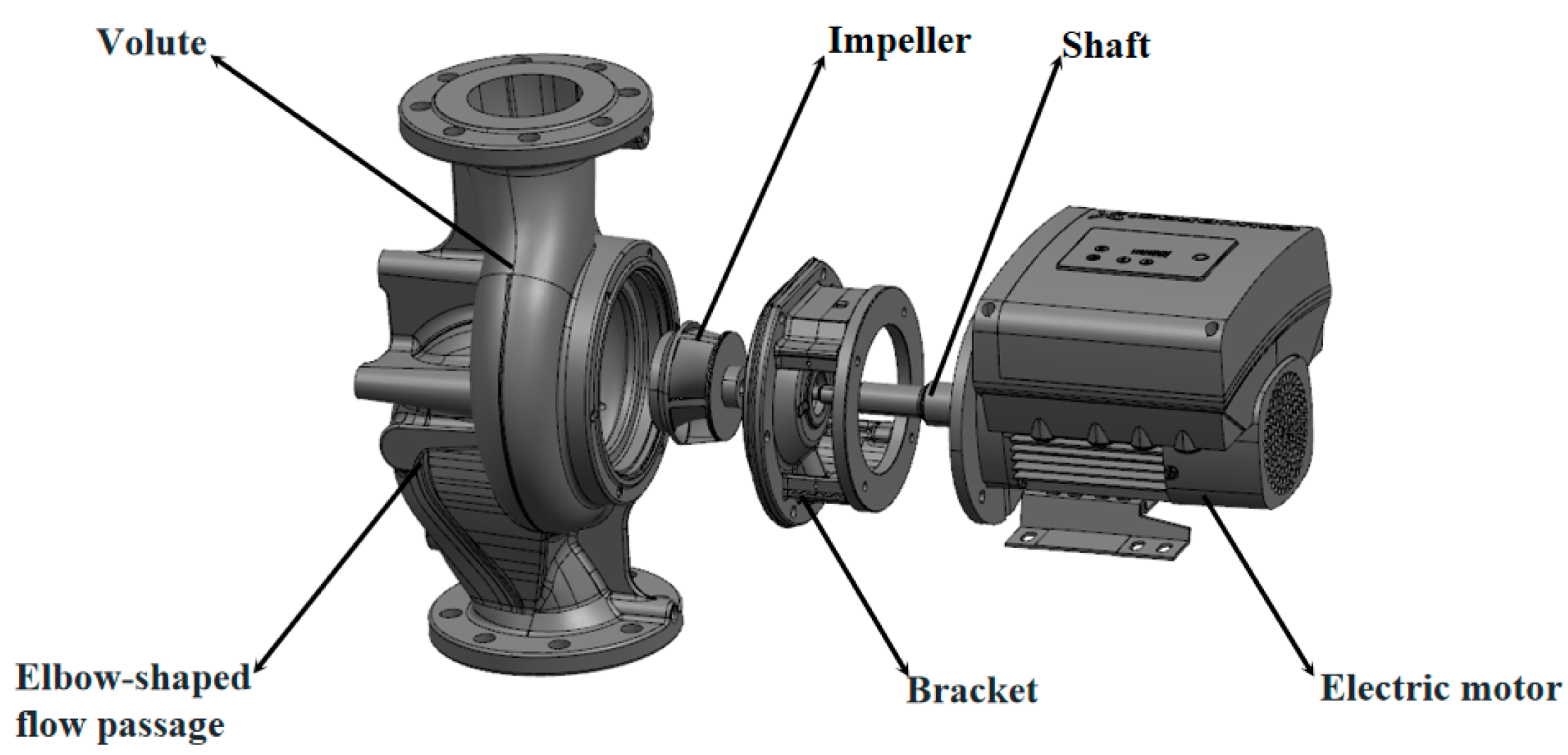
2.1. Visual Pump Model

As shown in Figure 1, the pipeline pump utilized in the study is a vertical single-stage single-suction centrifugal pump. The following are the fundamental parameters of the visual pipeline pump model: The pump body and motor are linked without solid support, with a designed flow rate of 55 m³/h, a head of 7.8 m, an impeller outer diameter of 94.7 mm, and a blade number of 5. The impeller speed is n = 2900 r/min (Teacher Shen Zhenhua supplied the pump shown in Figure 1).

2.2. Grid Division

ICEM CFD on the Workbench platform was used for hexahedral mesh partitioning.

The computational model is composed of the hydraulic domain of a vertical pipeline pump, mainly consisting of the elbow-shaped inlet passage, impeller, volute, and outlet passage.

The study employed ICEM CFD in ANSYS software (2020R2) to partition the computational model into blocks for meshing. During mesh partitioning, the elbow-shaped inlet and the volute tongue region tended to misalign, leading to negative grids. Hence, a non-structured grid was used for hexahedral meshing of the flow field, with local refinements in relevant regions. The water domain mesh is illustrated in Figure 2, and finite volume methods were employed to discretize the governing equations. The coupling of velocity and pressure utilized the SIMPLEC algorithm on collocated grids.

Five different types of meshes were generated by setting various maximum cell sizes, and mesh independence validation was conducted [12], as presented in

Table 1. Mesh independence verification.

Scheme	Number	H/m	η/%
1	5,744,853	6.54	66.07
2	6,983,475	6.89	68.87
3	8,032,376	7.10	70.66
4	10,062,836	7.12	70.92
5	14,235,754	7.11	70.34

. The head and efficiency of the pump were used as validation standards. The computational efficiency and head stabilized when the total number of grids in the computational domain exceeded 8 million. Considering time costs and computational resources, Scheme 4 was chosen for subsequent calculations, with a total grid count of 10,062,836.

2.3. Turbulence Model and Boundary Condition Settings

Steady numerical simulations were conducted using ANSYS CFX 2020R2 software to obtain the pump’s external performance and internal flow characteristics. Water at 25 ℃ was considered the medium for internal flow. The continuity equation and the Reynolds-Averaged Navier-Stokes (RANS) equation were used as the governing equations, as shown in Equations (1) and (2), respectively. The Shear Stress Transport (SST) k-ω model was employed to better describe turbulent behavior across different scales; hence, the SST model was used to solve the N-S equations. The SST k-ω turbulence equations include kinetic energy and characteristic scale equations as depicted in Equations (3) and (4), respectively. Inlet boundary conditions were set as flow inlet, and the outlet boundary was set as pressure outlet with a pressure of P = 1.01 × 10⁵ Pa. The solid wall was set as a “no-slip boundary” condition, while the interface between the rotating and stationary domains was set as “Frozen rotor” and “None,” respectively. The solver settings were configured with high-order solution accuracy, a maximum of 2000 iterations, and a convergence criterion of 10⁻⁵.

The governing equations were as follows:

$$\frac{\mathsf{\partial }\left(u_i\right)}{\mathsf{\partial }{x}_i}=0$$

(1)

$$\rho \frac{\mathsf{\partial }\left(u_i\right)}{\mathsf{\partial }t}+\rho u_j\frac{\mathsf{\partial }\left(u_i\right)}{\mathsf{\partial }{x}_j}=\rho F_i-\frac{\mathsf{\partial }p}{\mathsf{\partial }{x}_i}+\mu \frac{{\mathsf{\partial }}^2{u}_i}{\mathsf{\partial }{x}_i\mathsf{\partial }{x}_j}$$

(2)

$u_i$: instantaneous value of velocity in the $i$ direction; $x_i$: coordinates; $\rho$: fluid density; $p$: fluid pressure; $F_i$: mass force; and $\mu$: dynamic viscosity.

The equation for kinetic energy $k$ is as follows:

$$\frac{\mathsf{\partial }\left(\rho k\right)}{\mathsf{\partial }t}+\frac{\mathsf{\partial }\left(\rho u_{j}k\right)}{\mathsf{\partial }{x}_j}=\frac{\mathsf{\partial }}{\mathsf{\partial }{x}_j}\left[\left(\mu +{\sigma }_k{\mu }_t\right)\frac{\mathsf{\partial }k}{\mathsf{\partial }{x}_j}\right]-\rho \epsilon -\beta \ast \rho k\omega$$

(3)

$\rho$: fluid density; $t$: time; $x_j$: spatial coordinates; ${\mu }_i$: velocity component; $\mu$: dynamic viscosity; ${\mu }_t$: turbulent viscosity; ${\sigma }_k$: the effectiveness function of $k$; ε: the dissipation rate of $k$; and $\beta$: the coupling coefficient between $k$ and $\omega$.

The characteristic length scale equation is as follows:

$$\frac{\mathsf{\partial }\left(\rho \omega \right)}{\mathsf{\partial }t}+\frac{\mathsf{\partial }\left(\rho u_j\omega \right)}{\mathsf{\partial }{x}_j}=\frac{\mathsf{\partial }}{\mathsf{\partial }{x}_j}\left[\left(\mu +{\sigma }_{\omega }{\mu }_t\right)\frac{\mathsf{\partial }\omega }{\mathsf{\partial }{x}_j}\right]-\alpha \frac{\omega }{k}\frac{\mathsf{\partial }k}{\mathsf{\partial }{x}_j}\frac{\mathsf{\partial }\omega }{\mathsf{\partial }{x}_j}-\beta \ast \rho k{\omega }^2$$

(4)

$\alpha$: the model parameter; ${\sigma }_{\omega }$: the effectiveness function of $\omega$; and $\beta$: the coupling coefficient of ω dissipation rate.

3. Optimization Process

The flowchart of the elbow channel optimization design based on the Sand Cat Swarm Optimization BP neural network is shown in Figure 3. With the efficiency of the vertical pipeline pump under design conditions as the optimization goal, the main design parameters of the elbow inlet channel were determined by the xy coordinate values at the section’s midpoint using B-spline curve fitting of the channel profile combined with CREO parametric 3D modeling. Finally, the experimental design identified four significant elbow inlet channel factors. By using a uniform experimental design [13], the elbow inlet channel design scheme was created within the design range, and numerical simulation was used to determine the pump efficiency. The approximate mathematical model of efficiency and four significant sample factors were established by optimizing the BP neural network with the Sand Cat Swarm algorithm. The approximate mathematical model was globally optimized by a genetic algorithm. Finally, the design parameters and optimization objectives of the optimal elbow inlet channel were obtained.

3.1. Elbow Inlet Channel Parameterization Method

The outer contour of the elbow inlet channel is parameterized using weight screening processing of the profile parameters, which is more conducive to reducing the complexity of the agent model, such as an artificial neural network or kriging [14], and improving accuracy and calculation time.

The geometric characteristics impacting the hydraulic performance of the elbow inlet channel are mainly determined by the geometric shape of the profile and flow cross section; thus, the parametric design factor variables are primarily chosen from these two components. When two section forms and channel profiles are defined, CREO may generate three-dimensional geometry with a uniform transition. The flow channel profile is composed of spline curve parameterization, and the geometric parameters of the A-A and B-B sections, which are easily modifiable, are chosen to study the flow cross section.

The shape of the elbow flow line is determined by fitting 6th power B-spline curves through the midpoint of the section. As shown in Figure 4, the direction of the flow line is controlled by changing the midpoint of the section on the middle flow line (taking into account the internal flow field and the actual installation needs, the x coordinate of point D is fixed, the y coordinate of point D is changed, and the y coordinate of the remaining four points is fixed and the x coordinate value is changed). The section shape is determined by the section length and transition angle. There are nine initial parameters in total. CREO 9.0 parameterizes the nine parameters in order to regulate the profile of the elbow inlet channel, in which the inlet and outflow are fixed.

The original data for the elbow variables referred to relevant materials such as Design and Computational Method of Pump Elbow Inlet Flow and Modern Pumps Theory and Design [15,16,17,18]. The upper and lower limits of the design parameters are shown in

Table 2. Upper and lower limits of the design parameters.

Variable	Upper Limit	Lower Limit
DS-B	56	58
DS-C	49	51
DS-D	180	195
DS-E	80	83
DS-G	138	144
RA	10	25
RB	35	40
LA	90	110
LB	100	120

.

3.2. Screening of Significant Variables

The objective of factororial design is to use a limited number of trials to examine the impact of several factors simultaneously. The P2 experimental design [19] method is used for preliminary factor screening when there are too many potential factors as a result of the excessive parameters used in this study. This allows for an effective screening process to identify the primary affecting factors within a limited number of experiments. Part of the two-level experiment was designed with Minitab software (Minitab2021), the design accuracy was set to level IV, and a total of 32 groups of experiments were randomized. According to the design values of part of the two-level experiments, three-dimensional parametric modeling was carried out for 32 groups of experiments. In order to reduce the influence of mesh differences in subsequent analysis, the same mesh size parameters were set. Since the experiment is implemented using the CFD method, there is no human error or accidental error, and the simulation efficiency is used as the evaluation index of the P2 test.

To comprehensively consider the significant characteristics of various factors, Minitab generated a half-normal plot for each factor’s effects (as shown in Figure 5). From the graph, the x-axis represents the absolute values of effects, while the y-axis indicates the probability percentage. The significance level α is set at 0.05, and significant effects are identified in the plot using corresponding letter codes. Analyzing the physical interpretation of the semi-normal distribution diagram, factor H deviates farthest from the main trend, indicating its maximal impact among the factors. Effects located further away from the zero point on the x-axis exhibit larger magnitude values, suggesting greater statistical significance. Similarly, it can be concluded that the effect order of factors is: H > E > J > B > C, and the corresponding factors are: LA > DS-G > LB > DS-C > DS-D.

Since the aforementioned experiments only focused on the relationship between individual factors and efficiency, the half-normal plot reflects the relationship between the mean values of factors and response values. However, this does not entirely describe the response values. Therefore, in this paper, to eliminate the impact of interactions between dual or multiple factors, two methods, namely P-B experimental design and MATLAB multi-factor analysis of variance, were employed to comprehensively screen out significant factors. These were used to analyze the degree of influence of nine parameters on pump efficiency, considering a significance level α of 0.05.

Table 3. Comparison of p-values of efficiency-influencing factors.

Factor	P-B Test	Multivariate Analysis of Variance
DS-B	0.578	0.631
DS-C	0.0314	0.0275
DS-D	0.0434	0.344
DS-E	0.694	0.0563
DS-G	0.0624	0.0415
RA	0.144	0.087
RB	0.513	0.553
LA	0.0455	0.0233
LB	0.421	0.472

compares the probability values (p-values) from the P-B experimental design and multi-factor analysis of variance. Smaller p-values indicate a greater and more significant impact on efficiency.

According to the size of the p-value in the head P-B test, the first 6 digits are taken from small to large: DS_C < DS_D < LA < DS_G < RA < LB; Similarly, the first 6 positions from small to large in the multivariate analysis of variance are taken as follows: LA < DS-C < DS-G < DS-E < RA < DS-D. The results of the two methods are generally consistent and can be verified by each other.

According to the significance analysis of the design of the two-level factorial experiment in Table 3 and Part P2, the overlapping factors in 6 of them were selected, so that DS_C, DS_D, DS_G, and LA were determined as the optimized significant factors. According to the actual situation of the original pump model, the value range of each significant factor was determined, respectively: DS-C (80,88), DS-D (110,140), DS-G (160,175), and LA (20,40).

3.3. Approximate Model Establishment (BP Neural Network Improved Based on the Sand Cat Swarm Algorithm)

3.3.1. Sand Cat Swarm Algorithm

Sand Cat Swarm Optimization (SCSO) is a new meta-heuristic algorithm proposed by Amir Seyyedabbasi and Farzad Kiani in 2022. The algorithm is an intelligent optimization algorithm that imitates the survival behavior of sand cats in nature. The sand cat, which widely lives near the Sahara Desert in Africa, can capture 10% more food at night than the ordinary cat. This is attributed to their exceptional ability to detect low-frequency noises and their special population renewal mode, which guarantees both faster convergence and superior optimization [20]. SCSO simulates two main behaviors of the sand cat in the population renewal mode: searching for prey and attacking prey.

(1)

Search for prey (exploration)

The sand cat’s hearing capacity for low-frequency detection is beneficial to the sand cat swarm algorithm. The sand cat can detect low-frequency sound waves below 2 kHz. In order to progressively approach the prey without losing ground or skipping any steps, the sand cat’s ability value rG will linearly decline from 2 to 0 as the iteration process goes on.

Therefore, it is assumed that the sand cat’s sensitivity range is from 2 kHz to 0 for the purpose of searching for prey. SM simulates the sand cat’s hearing characteristics, of which the value is assumed to be 2. Certainly, it can be appropriately adjusted for different problems to determine the agent behavior’s speed, which demonstrates the adaptability and versatility of the proposed equation. The mathematical model mentioned above is described as follows:

$$r_G=s_M-(\frac{2\times s_M\times i_c}{i_{max}})$$

(5)

$i_c$: current iterations of the population; $i_{max}$: maximum number of iterations of the population.

The main parameter $R$ that controls the conversion between the exploration phase and the development phase can be defined as follows:

$$R=2\times r_G\times rand\left(\mathrm{0,1}\right)-r_G$$

(6)

Every sand cat has a randomly initialized search space that lies between the defined boundaries. To enable the search agent to discover new spaces within the search space, each current search agent’s location throughout the search process is based on a random location. Each sand cat has a distinct sensitivity range in order to prevent falling into local optimality, which can be defined as follows:

$$r=r_G\times rand\left(\mathrm{0,1}\right)$$

(7)

$r_G$: general sensitivity range that decreases linearly from 2 to 0; $r$: sensitivity range for each cat. In addition, r is used in the exploration or exploitation processes, while $r_G$ is used to guide the parameter $R$ to enable the transference between these processes.

With the SCSO algorithm, the sand cat can update its position based on the best possible solution, current position, and sensitivity range. It looks for additional prime prey positions and may locate a new local optimal position in the expanded search area. The position that it finds is between its current position and the prey position. Meanwhile, the algorithm’s low running costs and complexity are guaranteed by the randomization. The following is the mathematical model of the mentioned search process:

$$P(t+1)=r\cdot \left(P_{bc}\right(t)-rand(\mathrm{0,1})\cdot P_c(t\left)\right)$$

(8)

$P_{bc}$: optimal solution; $P_c$: current position; and $r$: sensitivity range.

(2)

Attack prey (exploitation)

Suppose that the sand cat’s sensitivity range is a circle. The direction of movement can be determined by a random angle on the circle; certainly, the remaining parameters stated in the formula are also valid for determining the direction of movement. Its value will be between −1 and 1, as the random angle selected is between 0 and 360. This allows every group member to move around the search space in a different circular direction. SCSO uses the Roulette Wheel Selection Algorithm to select a random angle for the sand cat so that it can approach the hunting position. In order to prevent falling into local optimality, SCSO uses a random angle. The random angle in the formula will improve the sand cat’s hunting and guidance, and the random position $P_{md}$ can guarantee that the sand cat can get close to the prey. The SCSO algorithm’s attacking process is mathematically represented, and its update mode is shown in Equations (9) and (10):

$$P_{md}=\left|rand\left(\mathrm{0,1}\right)\cdot P_b\left(t\right)-P_c\left(t\right)\right|,$$

(9)

$$P(t+1)=P_b\left(t\right)-r\cdot P_{md}\cdot \mathit{cos}(\theta )$$

(10)

$P_b$: best position (the best solution); $P_c$: current location; and $P_{md}$: random location.

(3)

Search and attack

The search and attack are switched using adaptive $r_G$ and R, so the SCSO can freely switch between the two modes. Since R depends on $r_G$, its range of fluctuation is also reduced. The value of R ranges from [−2$r_G$, 2$r_G$], and $r_G$ decreases linearly from 2 to 0. Therefore, the sand cat is set to attack when the parameter |R| ≤ 1, and its update mode is as follows:

$$P(t+1)=P_b\left(t\right)-r\cdot P_{md}\cdot \mathit{cos}(\theta )$$

(11)

When the boot parameter |R| > 1, its update mode is as follows:

$$P(t+1)=r\cdot \left(P_{bc}\right(t)-rand(\mathrm{0,1})\cdot P_c(t\left)\right)$$

(12)

3.3.2. BP Neural Network

The BP neural network is an artificial intelligence model based on artificial neurons to simulate a human brain neural network, which belongs to a kind of feedforward neural network consisting of an input layer, a hidden layer, and an output layer. It is characterized by the ability to train and optimize the network through a backpropagation algorithm to solve problems such as classification and regression. The schematic diagram of the neural network is shown in Figure 6.

Each circle represents a neuron. In the input layer, neurons are composed of input variables. In the hidden and output layers, neurons consist of input variables and activation functions. Specifically, the input variables are obtained by summing the linear transformation of all output variables from the preceding layer. These variables are then transformed through an activation function and serve as output variables inputted into the subsequent layer for computation.

(1)

In the process of signal forward transmission, assuming that the value of $ne{t}_i$ is input on the $i_{th}$ node of the hidden layer, its expression can be shown like this:

$$ne{t}_i=\sum _{j=1}^M{w}_{ij}{x}_j+{\theta }_i$$

(13)

The output of the ith neuron node of the hidden layer ${\theta }_i$, whose expression is shown in:

$$o_i=f(ne{t}_i)=f(\sum _{j=1}^M{w}_{ij}{x}_j+{\theta }_i)$$

(14)

Choosing the logsig function as the activation function for the hidden layer of the neural network, its expression is as follows:

$$y=\frac{1}{1+e^{-x}}$$

(15)

Using the purelin function as the linear activation function for the output layer of the neural network, its expression is as follows:

$$y=x$$

(16)

The expression for the input value of the kth neuron node in the output layer $ne{t}_k$ is shown in:

$$ne{t}_k=\sum ^q{w}_{ki}{y}_i+a_k=\sum _{i=1}^q{w}_{ki}f(\sum _{j=1}^M{w}_{ij}{x}_j+{\theta }_i)+a_k$$

(17)

The expression for the output of the kth neuron node in the output layer $o_k$ is shown in:

$$o_k=g\left(ne{t}_k\right)=g\left(\sum _{i=1}^q{w}_{ij}f\left(\sum _{j=1}^M{w}_{ij}{x}_j+{\theta }_i\right)+a_k\right)$$

(18)

(2)

Error Backpropagation Process

The process of error backpropagation involves obtaining the error value by subtracting the values of all neurons in the output layer of the training model from the actual values. This error value is then used to continuously adjust the weights and thresholds through backward propagation. Corrections are made to the direction and magnitude of the partial derivatives of the neuron weights and thresholds across layers based on the calculated error until the error reaches our predefined conditions, signaling the end of the training process.

The total error function $MSE$ is expressed in Equation (19):

$$MSE=\frac{1}{n}\sum _{k=1}^L(T_k-O_k{)}^2$$

(19)

The adjusted weights and thresholds corresponding to the input and output layers are shown in Equations (20)–(23):

$$\Delta w_{ki}=\eta \sum _{p=1}^p\sum _{k=1}^L({T^p}_k-{O^p}_k)\cdot g^{\prime }(ne{t}_k)\cdot y_i$$

(20)

$$\Delta {\theta }_i=\eta \sum _{p=1}^p\sum _{k=1}^L({T^p}_k-{O^p}_k)\cdot g^{\prime }(ne{t}_k)\cdot w_{ki}\cdot f^{\prime }(ne{t}_i)$$

(21)

$$\Delta a_k=\eta \sum _{p=1}^p\sum _{k=1}^L({T^p}_k-{O^p}_k)\cdot g^{\prime }(ne{t}_k)$$

(22)

$$\Delta w_{ki}=\eta \sum _{p=1}^p\sum _{k=1}^L({T^p}_k-{O^p}_k)\cdot g^{\prime }(ne{t}_k)\cdot w_{ki}\cdot f^{\prime }(ne{t}_i)$$

(23)

$w_{ij}$: the weight between the jth neuron node in the input layer and the ith neuron node in the hidden layer; $\raisebox{1ex}{$x$}\!\left/ \!\raisebox{-1ex}{$y$}\right.$: the input and output of the nodes, respectively; $w_{k_j}$: the weight between the ith neuron node in the hidden layer and the kth neuron node in the output layer; $x_j$: the input of the jth neuron node in the input layer; $i$: the threshold of the ith neuron node in the hidden layer; $f{\left(x\right)}_i$: the activation function of the hidden layer; ${\alpha }_k$: the threshold of the kth neuron node in the output layer; $g_{\left(x\right)}$: the linear activation function of the output layer; and $o_k$: the output of the kth neuron node in the output layer

3.3.3. Construction of the SCSO-BP Neural Network

To ensure the accuracy of the approximate model, this paper selects 50 sets of uniformly designed numerical simulation data to construct the sample space. A total of 70% of the samples (35 sets) are used to train the SCSOBP neural network using a uniform experimental design. Additionally, 30% of the samples (15 sets) are utilized to verify the accuracy of the neural network. The relevant settings of the BP neural network are as follows: The training function adopts the Levenberg-Marquardt (L-M) optimization algorithm Trainbr, and the node transfer functions use Logsig and Pureline for the logistic sigmoid and linear functions, respectively. The training loop iteration count is set to 1000, with a learning rate of 0.01, and the training objective minimum error is 0.00001. Normalization is performed using Mapminmax, and the performance function adopts the mean square error (MSE). Furthermore, the SCSO-BP neural network is designed with 4 nodes in the input layer, 9 nodes in the hidden layer, and 1 node in the output layer, where the output represents the efficiency at operating points. The preliminary establishment of a 4-9-1 neural network model is shown in Figure 6b.

Traditional BP neural networks often utilize gradient descent to search for weights and thresholds. They are sensitive to initial values, exhibit slow convergence, are prone to gradient vanishing, causing training difficulties, and can get trapped in local optima for non-convex optimization problems. The Sand Cat Swarm Optimization (SCSO) algorithm attempts to address the limitations of traditional gradient descent, enhancing the performance and robustness of optimization algorithms.

The essence of utilizing Sand Cat Swarm Optimization (SCSO) to optimize a backpropagation (BP) neural network is to mimic the behavior of sand cats in their food search process. Within the sand cat swarm, individuals seek optimal solutions based on their positions. Sand cats update their positions according to their locations and the surrounding environment, akin to adjusting the weights and thresholds within the neural network. This adjustment aims to reduce the predictive errors of conventional BP neural networks. Leveraging the search strategies and adaptability inherent in the SCSO algorithm (as represented by Equations (5)–(11)), it attempts various combinations of weights and thresholds to seek the most optimal parameters.

The specific methodology of optimizing weights and thresholds using the SCSO involves: initializing weights and thresholds, defining an error function, applying the SCSO algorithm for optimization, iteratively optimizing, and extracting optimal parameters. Figure 7 illustrates a portion of the SCSO algorithm’s code (position update of individuals).

This section represents the primary optimization loop. It utilizes a while loop iterating imax times. In each iteration, the positions of each search agent are updated. The optimizer employs logic to ensure that the agent’s positions remain within the defined search space (defined by lb and ub) and computes the agent’s fitness based on the optimization objective function (defined by fobj). The optimization process involves adjusting the agent’s positions and updating them based on the unique search and prey-attacking behaviors of the SCSO algorithm. As the iterations progress, the convergence curve records the best fitness value for each iteration. Finally, this optimization function returns three values: the best score, the best fit, and the convergence curve.

4. Results and Discussion

4.1. Test Verification

To validate the accuracy of the numerical simulation, an external characteristic experiment was conducted on the original model. The experiment was conducted at the closed test bench of the National Water Pump Product Quality Supervision and Inspection Center (Zhejiang), as depicted in Figure 8a. The impeller and pump casing were processed by Grandf Suzhou Co., Ltd., and the motor was provided by Professor Shen Zhenhua. The prototype pump test bench setup is shown in Figure 8b. The measurement error for head and efficiency was controlled within 0.5%, while the uncertainty in flow rate was maintained within 3%.

The performance of a pump is fundamentally indicated by its characteristic curves. The external characteristic experiment, which represents the pump’s entire flow rate performance, was derived from the external performance test system at the National Pump Testing Center. The experimental pump efficiency was calculated by converting the unit efficiency through the motor power factor. The formulas for calculating the head ($H$), shaft power, and efficiency using CFD numerical simulation are as follows:

$$H=(P2-P1)$$

(24)

$$N=\omega M$$

(25)

$$\eta =\rho gHQ/N$$

(26)

$P2$: the total pressure at the pump outlet; $P1$: the total pressure at the pump inlet; $\omega$: the angular velocity of the impeller; and $M$: the torque of the impeller.

The comparative chart of experimental tests and numerical simulation for the pump’s performance curve is depicted in Figure 9. Near the designed flow rate, the error between the efficiency test value and the calculated value is less than 6.5%. When the flow rate is 55 m³/h, the error between the efficiency calculation value and the test value is the largest, and the error is 6.43%. The error between the test and the calculated head value is less than 5%. When the flow rate is 40 m³/h, the error between the calculated head value and the test value is the largest, and the calculated head value and the test value are 10.23 and 9.79, respectively, with an error of 4.49%. It cannot be seen from the figure that the external characteristic test results and numerical simulation results have a good fit, indicating that the reliability of numerical calculation results near the optimal operating point is high. In this paper, the structural parameters of the design point are optimized and analyzed.

4.2. The Predictive Results and Comparative Analysis

The SCSO-BP neural network established an approximate predictive model between the four optimized variables and efficiency. Whether in the training or test set (Figure 10a,b), comparing the CFX calculated values with the predicted efficiency values before and after optimization using the BP neural network, the network’s predictive accuracy improved after using the SCSO algorithm, maintaining an error range within 5%. By comparing the sample errors in the test set, it is noticeable that, in contrast to the traditional unoptimized BP neural network, the error range became smaller with improved stability in error fluctuation in the BP neural network based on the CSCO enhancement. Therefore, it can be considered that the efficiency predictive model trained using the CSCO-BP neural network is accurate.

Using a genetic algorithm to optimize the optimized BP prediction model, the parameter data set after convergence is shown in

Table 4. Design parameter comparison.

Parameters	DS_C	DS_D	DS_G	LA	Efficiency/%	Head/m
Original scheme	82.64	129.12	174.99	22.0	0.721	8.023
Optimization scheme	85.77	129.14	164.44	33.1	0.758	8.624

:

4.3. Comparison of Flow Patterns in the Inlet

Based on the comparison of the model lines before and after optimization in Figure 11, the main change is observed in the transition angle between the middle streamline and the vertical section. Combining this with Table 4 for analysis: Although the distance of LA has increased, it still complies with the principle of linear gradient design for the inlet section and the relevant design standards [21]. The distance from the impeller’s centerline to the bottom plate of the inlet flow passage remains almost unchanged. This indicates that the optimized model has a minimal impact on the axial distribution uniformity of the outgoing flow, thus not causing significant hydraulic losses [22].

By observing the shape of the middle section of the elbow-shaped inlet before and after optimization, it is noticeable that the middle streamline of the optimized middle section appears smoother and more continuous compared to the original model. From the perspective of the upper and lower contour lines, the vertical angle at the inlet section of the upper and lower contour lines is smaller in the optimized version, mainly seen in the variation at point G. There is not a significant change in the angle of the profile lines near the outlet horizontal section before and after optimization.

In the optimized elbow-shaped inlet flow passage, the transition of streamlines between the elbow and the upstream and downstream flow components appears smoother. Particularly near the outlet section of the elbow, there is a more gradual curvature in the bend.

Due to the original model’s non-uniform curvature at the inlet section and the first bend, it led to certain levels of impact losses near the inlet, creating low-velocity regions as depicted in Figure 12. There was a significantly higher velocity gradient generated near the second bend in the original model compared to the optimized gradient. This impacted the flow state within the elbow-shaped inlet, causing uneven distribution within the pipeline. In the optimized model, there was a reduction in the velocity gradient at the bend, resulting in a more uniform velocity distribution across the mid-section. This improvement in flow conditions entering the impeller led to an overall enhancement in efficiency.

Due to a tapered section at the end of the original model’s elbow, observations of the optimized and pre-optimized elbow throat vector diagrams within the elbow inlet flow passage (as shown in Figure 13) reveal the presence of some secondary flow phenomena in the pre-optimized model, leading to poorer fluid velocity uniformity entering the impeller. The inlet flow passage of the original model generates a significant velocity gradient near the throat (as depicted in Figure 14). Following optimization, the velocity distribution near the throat becomes more uniform, with a noticeable reduction in velocity gradients. Additionally, in the optimized model, there is a decrease in secondary backflow phenomena at the edges of the impeller inlet, resulting in a more uniform flow distribution compared to the original model.

From Figure 15, it can be observed that there are significant differences in the static pressure distribution within the suction chamber before and after optimization, mainly evident at the inlet, the outlet, and points 1, 2, and 4. The gradient of static pressure decreases after optimization, reducing the area of high-pressure regions at points 1, 2, and 4. The static pressure distribution becomes less uniform at points 1 and 3, although the static pressure gradient decreases. Additionally, the static pressure gradient at point 5 of the optimized elbow inlet becomes more gradual.

Taking the inlet section, throat section, and outlet section of the elbow inlet flow passage to analyze the flow status before and after optimization, the flow status at the inlet remains largely unchanged. However, at the inlet section, the original model experiences higher impact losses along the flow passage wall, resulting in a significant velocity gradient at the throat. The original model’s surface transition is not smooth, creating more low-velocity areas on the outer side of the second bend. Along the passage from the throat section towards the elbow outlet section, more low-velocity areas accumulate on the middle and outer sides of the second bend, as shown in Figure 16a. This uneven flow does not uniformly enter the impeller, resulting in a tonsil-shaped velocity distribution at the outlet section, as shown in Figure 16b. This affects the flow state at the impeller inlet, ultimately impacting the overall pump efficiency. In contrast, the transition of the optimized model’s lines is smoother, reducing the impact losses between the fluid and the bend surface. The accumulation of low-speed regions decreases, lowering the velocity gradient at the throat section. This reduction mitigates the tonsil-shaped velocity distribution. The velocity distribution at the outlet section becomes more uniform, leading to an overall efficiency improvement of the pump under design conditions.

4.4. Performance Curve Comparison

Based on prior experimental validation and analysis, the stable and relatively low errors prove the reliability of the numerical simulation setup. Therefore, the comparative analysis of the performance curves was conducted using the numerical simulation data of the pipeline pump’s elbow-shaped inlet before and after optimization.

The comparison between the optimized and original models’ design parameters after convergence optimization is presented in Table 4. It shows that the throat section length (LA) had the most significant change, increasing by 50%. The other design parameters showed minor variations. This reaffirms that the throat section length can impact the impact losses at the elbow bend, resulting in a smoother and more uniform inlet flow velocity. The efficiency after optimization reached 75.8%, an improvement of 5.13% compared to the original model, while the head was 8.424, about 7.48% higher than the original model. The pump model’s external characteristic curves before and after optimization of the elbow-shaped inlet flow channel are depicted in Figure 17. Near the design flow point, both efficiency and head significantly improved. However, around low and high flow rates, as the internal flow states were already good before and after optimization, the efficiency only slightly increased. At low flow rates, there were higher impact losses at the elbow inlet, resulting in a lower head after optimization compared to the original model. Overall, the optimized pump showed enhanced overall efficiency and head, expanding its range of efficient operation.

5. Conclusions

• A SCSO-BP neural network has a better fit for network training, showing higher predictive accuracy in the improved BP neural network structure. The error fluctuations within the sample space were more stable, with a narrower range of fluctuations. The method presented in this paper can serve as a reference for multi-parameter optimization.
• The improved elbow inlet channel may operate in a wider range of high efficiency, and it has the greatest effect on the pump performance close to the design point.
• At points close to the design flow rate, the optimized model’s efficiency and head are greatly improved; under the design conditions, the efficiency increased by 5.13% and the head increased by 7.48%.
• The model’s profile on the bend pipe’s curvature transition is smoother, the low-speed area outside the appearance is smaller, the flow velocity distribution into the impeller is more uniform, and the secondary flow at the exit section’s edge is smaller after optimization, all of which improve the impeller’s fluid state. The elbow inlet channel fitting using spline curves is suggested as a source of inspiration for computer-aided parametric modeling. An efficient reference for multi-factor optimization and efficient design is provided by the suggested approach of collaborative optimization of the inlet flow channel, which is based on the SCSO-BP neural network and DOE experimental design.

References

1. Stephen, C.; Yuan, S.; Pei, J.; Cheng, G.X. Numerical Flow Prediction in Inlet Pipe of Vertical Inline Pump. ASME J. Fluids Eng. 2018, 140, 051201. [Google Scholar] [CrossRef]
2. Shi, W.; Li, Y.J.; Deng, D.S. Optimization design and numerical calculation of Elbow inlet channel. J. Fluid Mach. 2009, 37, 19–22. [Google Scholar]
3. Zhang, C.; Li, Y.J.; Jiang, H.Y. Simulation and experiment on Hydraulic Optimization of Elbow inlet channel. J. Drain. Irrig. Mach. Eng. 2016, 34, 860–866. [Google Scholar]
4. Semenova, A.V.; Chirkov, D.V.; Skorospelov, A.V.; Ustimenko, A.S.; Turuk, A.P.; Rigin, E.V.; Germanova, A.I. Optimization design of the elbow draft tube of the hydraulic turbine. IOP Conf. Ser. Earth Environ. Sci. 2022, 1079, 012028. [Google Scholar] [CrossRef]
5. Stanley, K.O.; Clune, J.; Lehman, J.; Miikkulainen, R. Designing neural networks through neuroevolution. Nat. Mach. Intell. 2019, 1, 24–35. [Google Scholar] [CrossRef]
6. Wang, Y.; Lu, C.; Zuo, C. Coal mine safety production forewarning based on improved BP neural network. Int. J. Min. Sci. Technol. 2015, 25, 319–324. [Google Scholar] [CrossRef]
7. Chen, M.J. An Improved BP Neural Network Algorithm and its Application. Appl. Mech. Mater. 2014, 543–547, 2120–2123. [Google Scholar] [CrossRef]
8. Guo, Y.; Li, G.; Chen, H.; Wang, J.; Guo, M.; Sun, S.; Hu, W. Optimized neural network-based fault diagnosis strategy for VRF system in heating mode using data mining. Appl. Therm. Eng. 2017, 125, 1402–1413. [Google Scholar] [CrossRef]
9. Gan, L.; Wang, Y.; Wang, B. Application of BP neural network in fault diagnosis of electric submersible pump Wells. Oil Drill. Prod. Technol. 2011, 33, 124–127. [Google Scholar]
10. Seyyedabbasi, A.; Kiani, F. Sand Cat swarm optimization: A nature-inspired algorithm to solve global optimization problem. Eng. Comput. 2022, 39, 2627–2651. [Google Scholar] [CrossRef]
11. Abkenar, S.M.S.; Stanley, S.D.; Miller, C.J.; Chase, D.V.; McElmurry, S.P. Evaluation of genetic algorithms using discrete and continuous methods for pump optimization of water distribution systems. Sustain. Comput. Inform. Syst. 2015, 8, 18–23. [Google Scholar]
12. Ferziger, J.H.; Perić, M.; Street, R.L. Computational Methods for Fluid Dynamics; Springer: Berlin/Heidelberg, Germany, 2019. [Google Scholar]
13. Fang, K.-T.; Liu, M.-Q.; Qin, H.; Zhou, Y.-D. Theory and Application of Uniform Experimental Designs; Springer: Singapore, 2018. [Google Scholar]
14. Jeong, S.; Murayama, M.; Yamamoto, K. Efficient optimization design method using kriging model. J. Aircr. 2005, 42, 413–420. [Google Scholar] [CrossRef]
15. Lu, W.G. Numerical Solution for Drawing Design of Large pump Elbow flow channel. Pump Technol. 1992, 1, 11–14. [Google Scholar]
16. Guan, X.F. Modern Pump Technical Manual. Astronautic Publishing House: Beijing, China, 1995. [Google Scholar]
17. Wang, Y.M.; Shi, S.T. Analysis and application of cross section of flow channel with large pump elbow. J. Jiangsu Agric. Univ. 1994, 15, 75–80. [Google Scholar]
18. Girdhar, P.; Moniz, O. Practical Centrifugal Pumps; Elsevier: Amsterdam, The Netherlands, 2011. [Google Scholar]
19. Liao, C.T.; Chai, F.S. Design and analysis of two-level factorial experiments with partial replication. Technometrics 2009, 51, 66–74. [Google Scholar] [CrossRef]
20. Wu, D.; Rao, H.; Wen, C.; Jia, H.; Liu, Q.; Abualigah, L. Modified Sand Cat Swarm Optimization Algorithm for Solving Constrained Engineering Optimization Problems. Mathematics 2022, 10, 4350. [Google Scholar] [CrossRef]
21. GB/T 50265-97; Design Code for Pumping Station. China Planning Press: Beijing, China, 1997.
22. Zhu, H.G.; Yuan, S.Q.; Liu, H.L. Numerical simulation of Influence of Elbow inlet Channel on Hydraulic Performance of vertical axial flow pump. Chin. J. Agric. Eng. 2006, 22, 6–9. [Google Scholar]
Figure 1. Structural diagram of the pipeline pump.
Water 16 00074 g001
Figure 2. Calculation domain grid of the (a) elbow inlet channel, (b) impeller, and (c) volute.
Water 16 00074 g002
Figure 3. Optimization flow chart.
Water 16 00074 g003
Figure 4. Schematic diagram of the parameterized contour factors.
Water 16 00074 g004
Figure 5. Half-normal plot of each factor.
Water 16 00074 g005
Figure 6. Schematic diagram of the BP neural network (a) neuron information transmission and (b) error backpropagation.
Water 16 00074 g006
Figure 7. Part of the optimized SCSO code.
Water 16 00074 g007
Figure 8. Closed test bench construction of the original pump visual model. (a) A closed test platform for comprehensive testing of pump performance; (b) a prototype pump visual model.
Water 16 00074 g008
Figure 9. Comparison of numerical simulation and test results.
Water 16 00074 g009
Figure 10. SCSO-BP approximation model and error comparison. (a) SCSO-BP efficiency prediction vs. CFD efficiency prediction; (b) comparison of efficiency predictions for the test set before and after improvement; (c) error comparison between the test sets for SCSO-BP and BP.
Water 16 00074 g010
Figure 11. Comparison of the inlet channel profile before and after optimization.
Water 16 00074 g011
Figure 12. Relative velocity comparison of the middle section under design conditions: (a) original model and (b) optimization model.
Water 16 00074 g012
Figure 13. Optimized elbow throat vector image before and after: (a) pre-optimization model and (b) optimized model.
Water 16 00074 g013
Figure 14. Comparison of the velocity gradient near the throat section before and after optimization: (a) pre-optimization model and (b) post-optimization model.
Water 16 00074 g014
Figure 15. Static pressure distribution of the section before and after optimization: (a) pre-optimization model and (b) post-optimization model.
Water 16 00074 g015
Figure 16. Comparison of velocity distribution at each section of the elbow inlet: (a) pre-optimization model and (b) post-optimization model.
Water 16 00074 g016
Figure 17. Comparison of external characteristics between the optimized and original models.
Water 16 00074 g017