Dynamic Behavior and Mechanism of Transient Fluid–Structure Interaction in Viscoelastic Pipes Based on Energy Analysis

Abstract

The term “viscoelastic pipe” refers to high polymer pipes that exhibit both elastic and viscoelastic properties. Owing to their widespread use in water transport systems, it is important to understand the transient flow characteristics of these materials for pipeline safety. Despite extensive research, these characteristics have not been sufficiently explored. This study evaluates the impact of friction models on the transient flow of viscoelastic pipes across various Reynolds numbers by employing an energy analysis approach. Given the complexity and computational demands of two-dimensional models, this paper compares the accuracy of one-dimensional and quasi-two-dimensional models. Notably, the superiority of the quasi-two-dimensional model in simulating viscoelastic pipelines is demonstrated. Owing to the interaction between pressure waves and fluid within viscoelastic pipes, fluid–structure coupling significantly attenuates pressure waves during transmission. These findings shed light on the constitutive properties of viscoelastic pipes and the influence of pipe wall friction models on transient hydraulic characteristics, building upon prior studies focused on elastic pipes. Nevertheless, numerous factors affecting transient flow in viscoelastic pipes remain unexplored. This paper suggests further analysis of strain effects, starting with temperature and pipe dynamics, to enhance the understanding of the coupling laws and flow mechanisms in viscoelastic pipelines.

1. Introduction

During water supply, accidental pump restarts, valve maloperations, natural disasters, or human operational errors may cause rapid changes in water flow velocity, leading to pressure fluctuations within pipelines [1]. When analyzing the transient flow of the metal pipe, the strain generated by the pipe is proportional to the stress, and hence, the viscosity of the pipe wall is ignored; the metal pipe is called an elastic pipe. Driven by recent advancements in material science, various polymers like polyvinyl chloride (PVC), high-density polyethylene (HDPE), polypropylene (PP), and polyethylene (PE) are increasingly used in long-distance water pipelines [2]. Pipes that are made of these high-polymer materials exhibit both elastic and viscous properties, differentiating them from purely elastic pipes and classifying them as viscoelastic pipes. However, in the current design of water supply pipelines in some areas, the viscoelastic effects of these materials are often neglected. Under transient flow conditions, viscoelastic materials exhibit not only instantaneous strains like elastic materials but also delayed strains that lag behind the applied stress [3].

Compared to the well-established field of transient flow in elastic pipelines, viscoelastic pipelines introduce additional complexities. Transient flow analysis in these systems must account for both the influence of unsteady friction and the viscoelastic effect of the pipe material. However, an in-depth understanding of the dynamic behavior of viscoelastic pipelines under transient flow remains elusive. Consequently, numerical calculation methods for transient flow in viscoelastic pipes are still under development [4]. The pioneering research on transient flow in viscoelastic pipelines has mainly focused on incorporating a viscoelastic term into the continuity equation to account for the delayed strain behavior of these materials. Gally et al. [5] were the first to introduce this mathematical model. Additionally, the Kelvin–Voigt (K–V) model was adopted as a viscoelastic pipeline constitutive model to simulate the delayed strain response.

In the process of analyzing the transient flow of viscoelastic pipes, it is necessary to choose the frictional model reasonably to solve the mathematical model of pressure fluctuation. Existing friction models may be categorized into one-dimensional and quasi-two-dimensional approaches. Considering the computational efficiency and simplicity, numerical simulations typically favor these two modeling approaches [6]. Common approximation methods for one-dimensional friction models often underestimate the true value. To address this, Wylie et al. [7] proposed a method to reduce the truncation error associated with second-order linear approximation. Other approximation methods include first-order and second-order linear approximations. Chen and Pu [8] and Liu and Pu [9] employed the dynamic friction coefficient method combined with the second-order approximation to calculate the quasi-steady friction model. The Brunone model [10] built upon the work of Daily et al. [11] by introducing the convection acceleration term. This term improves the model’s ability to replicate pressure fluctuation decay observed in experiments; therefore, the Brunone friction model is widely used. Guo and Gao [12] further modified the Brunone model for leak detection in pipelines.

These models showcase the ongoing development of more sophisticated approaches to capture transient behavior in fluid flow simulations. To overcome limitations inherent in independent friction models, scholars have proposed two-dimensional and quasi-two-dimensional models, which leverage the assumption of axial symmetry in the pipeline flow field. These models combine the continuity equation with axial and radial momentum equations to calculate the instantaneous two-dimensional velocity and pressure fields within the pipeline.

Two-dimensional (2D) models offer a detailed understanding of flow dynamics but are computationally expensive and possess limited practical application. To address this, a simplified quasi-two-dimensional (quasi-2D) model built upon specific assumptions has been proposed. These assumptions include neglecting the radial velocity component and its derivative in the momentum equation, considering only pipeline pressure and disregarding the convection term for the axial stress in the momentum equation, and finally, ignoring the stress term in the radial momentum equation, which leads to a constant pressure across the cross section in the radial direction. By incorporating these simplifications, various methods have been developed to derive quasi-2D transient flow control equations for pipelines.

Ohmi et al. [13] established a time-mean quasi-2D transient flow control equation. Vardy and Hwang [14] proposed a novel approach to model transient flow using a quasi-2D framework. Their method involved discretizing the pipeline into a series of coaxial cylindrical control volumes with varying radial thicknesses. Each control body served as a basis for formulating the governing transient flow equation. The researchers then separated this equation into two distinct parts: a hyperbolic wave component and a parabolic diffusion component. The commonly used numerical method is the characteristic line method (Method of Characteristics, MOC). They calculated the hyperbolic wave part of the quasi-2D pipeline transient flow equation using the MOC method and employed the central difference method to solve the parabolic diffusion part of the transient flow equation. Finally, to enhance the model’s accuracy and stability, they incorporated a five-region algebraic turbulence model to calculate the Reynolds stress term in the momentum equation.

Duan et al. [15] combined theoretical analysis and numerical calculations to study the impact of unsteady friction and pipeline viscoelasticity on the attenuation of pressure fluctuations in transient flow. Their findings suggest that both factors initially affect pressure waves, but with time, the viscoelasticity effects become dominant. Pezzinga et al. [16] conducted experimental research on the dynamic response of an HDPE pipeline under a transient flow. They used the experimental results to validate and compare the numerical simulation parameters of different friction models and investigated the relationship between the viscoelastic pipeline’s mechanical parameters and the transient flow pressure wave period. Through experimental verification and analysis, they concluded that while the delay time was related to the pipeline length, the elastic modulus was independent of it. They also observed a linear relationship between the elastic modulus and wave period. Wahba [17] employed dimensional analysis to identify dimensionless parameters affecting the governing equation of transient flow in a viscoelastic pipeline under laminar flow conditions, investigating its 2D characteristics. Meniconi et al. [18] utilized a two-dimensional k–ε turbulence model to infer the dimensionless parameters related to Reynolds number (Re) and pipeline viscoelasticity. They then studied the effects of these parameters on pressure fluctuations, wall shear stress, velocity distribution, turbulence generation, and dissipation. The results show that a convolutional unsteady friction model that uses the frozen eddy viscosity hypothesis and R-0 has an accuracy that decreases with time.

As aforementioned, the transient flow analysis of viscoelastic pipelines has always focused on two aspects: the friction model and the viscoelastic effect of the pipeline. According to Wahba [17] and Meniconi et al. [18], the Reynolds number is one of the factors that affects the transient flow of a viscoelastic pipeline. Additionally, evolving research suggests that the viscoelastic constitutive parameter may not solely represent energy dissipation but rather might involve the energy transfer between the fluid and pipe wall, as noted by Duan et al. [19]. This emphasizes the increasing recognition of fluid–structure coupling characteristics as a crucial factor in analyzing transient flow in viscoelastic pipes. However, because the numerical simulation of transient flow is difficult and the accuracy is difficult to guarantee, the related problems need to be further studied.

Energy analysis methods have been widely used to explore transient flow phenomena in viscoelastic pipelines. Scholars have partially examined and discussed the hydraulic transient mechanical behavior in PVC and HDPE pipes by observing changes in the kinetic and elastic energies of the fluid within the pipes. Building upon previous work to enhance the energy analysis method [20], this study utilizes this approach to investigate the combined effects of friction models, viscoelastic constitutive characteristics, and Re on transient flow behavior in viscoelastic pipelines. Wu et al. [21] conducted a comprehensive analysis from the model derivation to the theoretical analysis and parameter verification for viscoelastic quasi-two-dimensional models. The article primarily focuses on the impact of viscoelastic constitutive effects on transient delay strain. However, the article does not discuss the energy analysis of viscoelastic pipe transient flow under different friction models, and the proportional relationship of various work performed at different Reynolds numbers is not analyzed in this article. Here, we further explored the mechanical characteristics of fluid–structure coupling during the transient flow processes. Our analysis involves three key steps. First, we compare transient flow in both elastic and viscoelastic pipes. Second, we build upon the existing two-dimensional energy equation for viscoelastic pipe transient flow to evaluate the work conducted by different friction models and their accuracy. Finally, we delve into the relationship between the friction model and the viscoelastic effect. By elucidating the dynamic behavior and evolution mechanism of transient fluid–structure coupling, this research aims to contribute to a more comprehensive understanding of transient flow phenomena in viscoelastic pipelines.

2. Methods and Models

2.1. Mathematical Model

Unlike elastic pipelines, viscoelastic pipelines exhibit both elastic and viscous behavior during transient flow. This section provides a detailed explanation of the equation derived from the elastic water column theory with the following assumptions:

(1)

Full pipe flow. The pipeline is completely filled with liquid, maintaining a constant average flow rate across any pipeline section throughout the process.

(2)

The most basic friction equation is used because of the comparison of friction models. The frictional resistance due to the pipe walls is calculated using the Darcy–Weisbach equation.

$$h_f=\lambda \frac{l}{D}\frac{v^2}{2g}$$

(1)

where $h_f$ is frictional head loss; $\lambda$ is friction coefficient along the course (N/m²); l is pipe length (m); D is pipe diameter (m); v is mean velocity in tube (m/s); g is gravitational acceleration (m/s²).

(3)

To disregard the inherent characteristics of the material, the changes caused by the heterogeneity of the material are overlooked. The pipeline material is assumed to be homogeneous and isotropic, ensuring uniformity to prevent it from functioning as a gravity flow pipe.

(4)

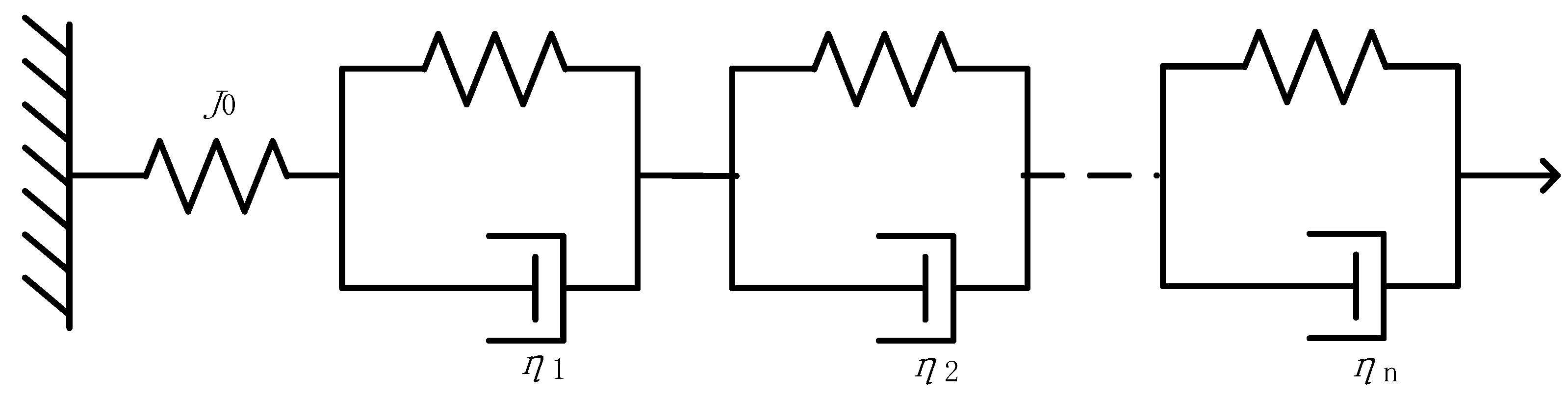
To streamline the analytical and solution models, linear viscoelastic behavior is assumed. This implies that the tube wall reacts linearly to transient flow excitation, where its stress response is directly proportional to the applied strain.

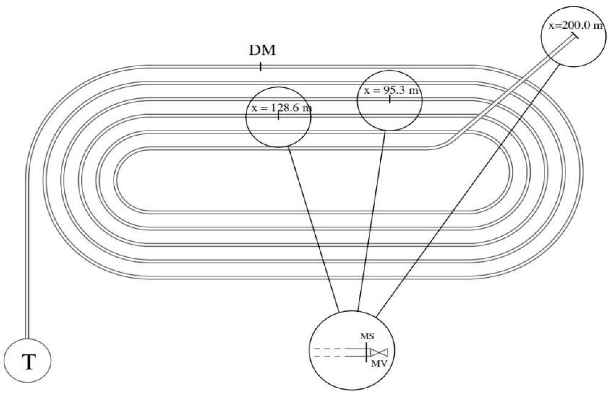
By incorporating these assumptions, the governing continuous equation for the transient flow in a viscoelastic pipeline is established as:

$$\frac{\partial p}{\partial t}+\rho a^2(\frac{\partial V}{\partial x}+2\frac{d{\epsilon }_r}{dt})=0$$

(2)

where ${\epsilon }_r$ is the delayed strain; $\rho$ is the liquid density (kg/m³); a is the wave velocity (m/s); p is the pressure (N); t is the time (s); and x is the distance (m).

The motion equation for the transient flow in a viscoelastic pipeline is defined as:

$$\rho \frac{\partial V}{\partial t}+\frac{\partial p}{\partial x}+\frac{{\tau }_w}{D}=0$$

(3)

where ${\tau }_w$ is the wall shear stress (Pa).

The key distinction between Equations (2) and (3) and the basic equation for transient flow in elastic pipes lies in the inclusion of a constitutive equation to account for the viscoelastic behavior of the pipe material. Polymeric materials exhibit both elastic and viscous characteristics, typically modeled using combinations of spring and dashpot (fluidic dampers) to account for the viscoelastic effect. Common mechanical models include the Maxwell, Voigt, and Maxwell–Weichert models and K–V models. The generalized K–V model represents a simple yet widely used approach [11]. It consists of a spring connected in series with a dashpot, comprising n K–V components, as illustrated in Figure 1.

This configuration captures the essential features of viscoelasticity: the spring represents the elastic response, and the dashpot reflects the viscous behavior. The constitutive curve of a viscoelastic pipeline based on the generalized K–V model is determined as follows:

$$J(t)=J_0+{\displaystyle \sum _{k=1}^{N_{KV}}{J}_k(1-e^{-\frac{t}{{\tau }_k}})}$$

(4)

where $J_k$ is the creep compliance of the kth element (m²/N), $J_k=1/E_k$ ($E_k$ is the elasticity modulus of the kth element (N/m²)); ${\tau }_k$ is the relaxation time of the kth element (s); $J_0$ is the instantaneous creep compliance (m²/N); $J\left(t\right)$ is the creep function.

Viscoelastic pipes exhibit strain under transient flow conditions. The Boltzmann superposition principle [22] states that the total strain (ε) of a linear viscoelastic material under a series of independent stresses σ(t) is the sum of the individual strains caused by each stress. This principle is mathematically expressed as

$$\epsilon (t)=J_0\sigma (t)+{\displaystyle {\int }_0^t\sigma (t-u)\frac{\partial J(u)}{\partial t}du}$$

(5)

where $\epsilon (t)$ is total strain as a function of time; $\sigma (t)$ is the stress at time t; and $J(u)$ is the creep function at time u.

The stress of the viscoelastic pipes can be calculated as

$$\sigma =\frac{\alpha \Delta pD}{2e}$$

(6)

where $\alpha$ is the wall constraint coefficient.

2.2. Physical Model

The physical model used in this study, shown in Figure 2, was derived from previous research by Keramat et al. [23]. The rationale behind selecting this experiment stems from its alignment with the simulation requirements. Additionally, as a pivotal experiment concerning the transient flow of elastic pipelines during the study period, it ensures the authenticity of the experimental data. The pressure pipe used in our model experiment was a high-density HDPE pipe with a 93.3 mm inner diameter, 8.1 mm wall thickness, and 200 m length; the fluid used is water, with a viscosity of 0.9142 × 10⁻³ (Pa·s). For the elastic pipe simulation, the viscoelastic term has been excluded from the calculations. The upstream end of the pipeline was equipped with a pressure tank to maintain constant pressure, while the downstream end utilized pneumatic valves that could be rapidly closed to introduce transient flow. Additional experimental parameters are explained in detail in

Table 1. Experimental parameters.

Number	Rate of Flow (L/s)	Reynolds Number	HT,0 (m)	C1 (×10−2 m/s)	C2 (×10−3 m/s2)	C3 (×10−5 m/s2)	Valve Shutdown Time (s)
1	1	13,900	21.63	2.32	−0.685	0.925	0.0875
2	2.04	28,400	21.13	5.03	−1.52	2.4	0.0752
3	2.95	41,000	20.74	6.33	−1.65	2.33	0.1188
4	4.03	56,000	20.34	7.93	−1.82	2.27	0.1575
5	5.02	69,700	19.82	9.37	−2.1	2.49	0.1533

.

The variation in the upstream pressure boundary values can be expressed as follows:

$$H_{\tau }=H_{t,0}+C_1{t}_1^{\prime }+C_2{t}_2^{\prime }+C_3{t}_3^{\prime }$$

(7)

where $t_i^{\prime }$ is a time parameter, $t\prime =t-L/a$; $L$ is pipe length (m), and $H$ is head pressure (m).

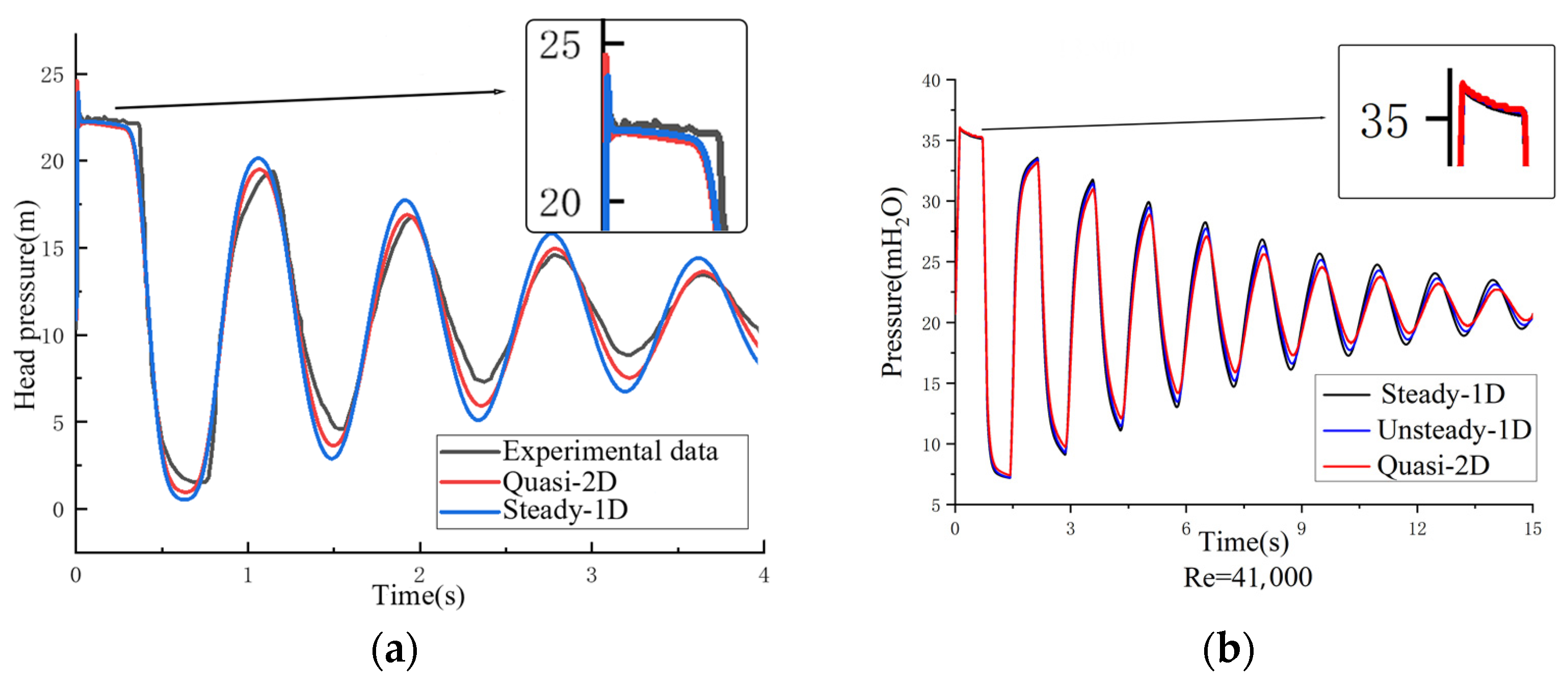
2.3. Comparison of Experiments on Different Friction Models

To assess the impact of frictional models and viscoelastic constitutive effects on transient flows, it is important to identify the optimal frictional model [24]. To achieve this, the experimental model and parameters were compared and analyzed alongside the available literature. The experiment utilized low-density polyethylene pipe, with an inner diameter of 41.6 mm and a wall thickness of 4.2 mm. The test platform, depicted in Figure 3, comprised three components––a pressure tank, a horizontally positioned p1pe, and a fast valve installed at a distance of 43.1 m from the pressure tank. The upstream pressure tank maintained a constant pressure, while the downstream fast valve generated transient flow excitation.

The experimental parameters are listed in

Table 2. Simulation parameters.

Number	Temperature (°C)	Initial Pressure (105 Pa)	Initial Flow Rate (m/s)	Kinetic Viscosity (10−i m2/s)	Reynolds Number	Volume Modulus (109 Pa)	Water Density (kg/m3)
1	25	1.0661	0.55	0.892	25,650	2.24	997.1

. One-dimensional steady-state and quasi-2D models were used for the transient flow numerical simulation to obtain pressure fluctuation curves at the designated pressure measurement point.

3. Results and Discussion

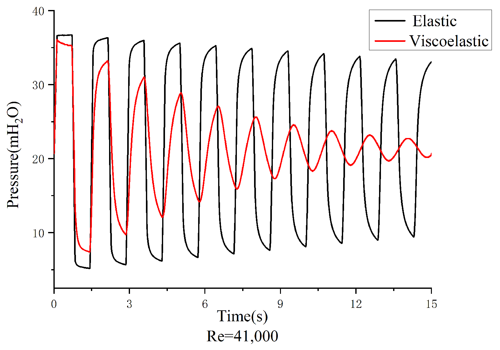
3.1. Influence of Pipe Types on Transient Flow

To analyze the difference between the transient flows in elastic and viscoelastic pipelines under excitation, we modeled pressure fluctuations. The model in Figure 2, combined with the mathematical model, was used to numerically solve the transient flows in elastic and viscoelastic pipelines, and the simulation results are shown in Figure 4.

The results indicate that the pressure fluctuation trend is the same at different Re; however, the generated peak pressure increases with an increase in the Re. The transient flow pressure calculated according to the elastic pipeline model has larger oscillation amplitude, higher frequency, and slower attenuation than that calculated by the viscoelastic pipeline model. Viscoelastic pipes exhibited an evident stress-delay effect.

As shown in Figure 5 (e.g., Re = 41,000), although the transient flow pressure of the elastic model decayed slowly, the maximum pressure was similar to that calculated using the quasi-2D viscoelastic pipeline model, and the difference increased as Re increased. During the transient flow in the viscoelastic pipeline, the first wave peak’s maximum pressure energy was not absorbed by the viscoelastic material. This phenomenon may be attributed to the limited responsiveness of the viscoelastic material owning to the short response time. The pressure fluctuation attenuates due to the viscoelastic effect’s energy absorption and storage, which manifests microscopic strains and small deformations within the pipeline material. Based on these observations, it can be concluded that the maximum water hammer pressure peak can be estimated using the elastic pipeline transient flow model for analysis purposes. However, for a quantitative understanding of pressure fluctuation attenuation, it is important to fully consider the crucial role of the viscoelastic delay effect in energy dissipation during the pipeline’s transient flow.

3.2. Effect of Friction Model on Transient Flow in Viscoelastic Pipes

3.2.1. Two-Dimensional Energy Equation for Transient Flow in Viscoelastic Pipeline

The establishment of the quasi-two-dimensional viscoelastic transient flow model neglects the radial velocity component and its derivative, the convection term, and the stress term of the radial momentum equation. Therefore, it is necessary to establish a two-dimensional energy equation before analyzing the performance of the frictional model in characterizing the transient flow of a viscoelastic pipeline. The mass conservation and momentum equations of the quasi-2D transient flow equation for viscoelastic pipelines are defined as follows:

$$\frac{g}{a^2}\frac{\partial H}{\partial t}+\frac{\partial u}{\partial x}+\frac{1}{r}\frac{\partial (rv)}{\partial r}=0$$

(8)

$$\frac{\partial u}{\partial t}+g\frac{\partial H}{\partial x}-\frac{1}{\rho r}\frac{\partial (r\tau )}{\partial r}=0$$

(9)

where u is the axial flow rate of fluid (m/s); r is radial distance; $\tau$ is the shearing stress.

Integrating the basic differential equations yields the energy equation for the quasi-2D model. However, owing to the presence of radial flow velocity in this model, radial integration becomes necessary alongside axial integration when calculating quantities related to flow velocity. Consequently, the total energy equation is expressed as follows [21]:

$$\frac{dU}{dt}+\frac{dT}{dt}+D_f+W_E+W_P=0$$

(10)

where $U$ is the internal energy of the system (J), defined as

$$U=\frac{\rho g^{2}Ar}{2a^2}{\displaystyle {\int }_0^L{H}^2}(x,t)dx$$

(11)

Here, $T$ is the kinetic energy of system (J), defined as

$$T(t)=\frac{\pi \rho Dg}{4}\frac{d{\displaystyle {\int }_0^L{\displaystyle {\int }_0^{\frac{D}{2}}{u}^{2}drdx}}}{dt}$$

(12)

where $D_f$ is total friction work in the system (J/s), calculated as

$$D_f(t)=\frac{\pi D}{2}{\displaystyle {\int }_0^L{\displaystyle {\int }_0^{D/2}\frac{u}{r}\frac{\partial (r\tau )}{\partial r}}drdx}$$

(13)

Here, $W_E$ is the work performed at both ends of the pipe (J/s) and is calculated as

$$W_E=\frac{\pi \rho Dg}{2}{\displaystyle {\int }_0^{D/2}[u(L,t)H(L,t)-u(0,t)H(0,t)]dr}$$

(14)

where $W_p$ is the work performed by the tube wall (J/s) and is calculated as

$$W_P=2\rho Ag{\displaystyle {\int }_0^{L}H\frac{\partial \epsilon }{\partial t}dx}$$

(15)

Additionally, W_P can be expressed as follows after the introduction of the radial flux:

$$W_P=\rho g{\displaystyle {\int }_0^{L}H(x,t)q_r(x,t)}dx$$

(16)

where $q_r$ is the radial flux; the derivation is provided in Appendix A.

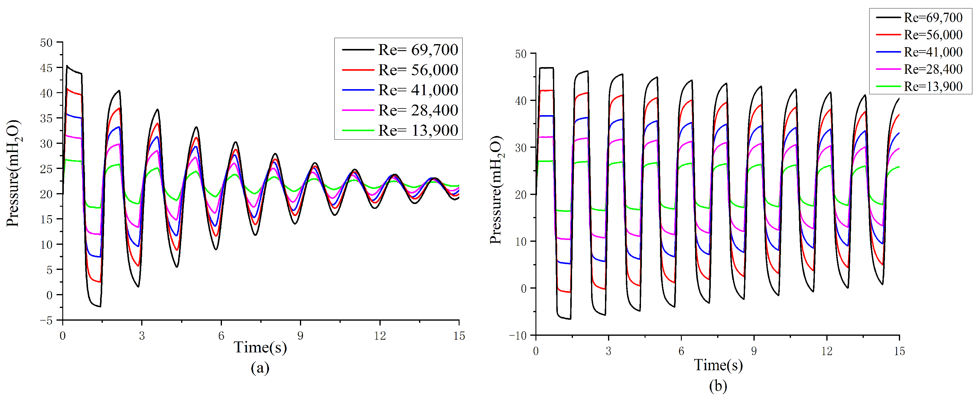
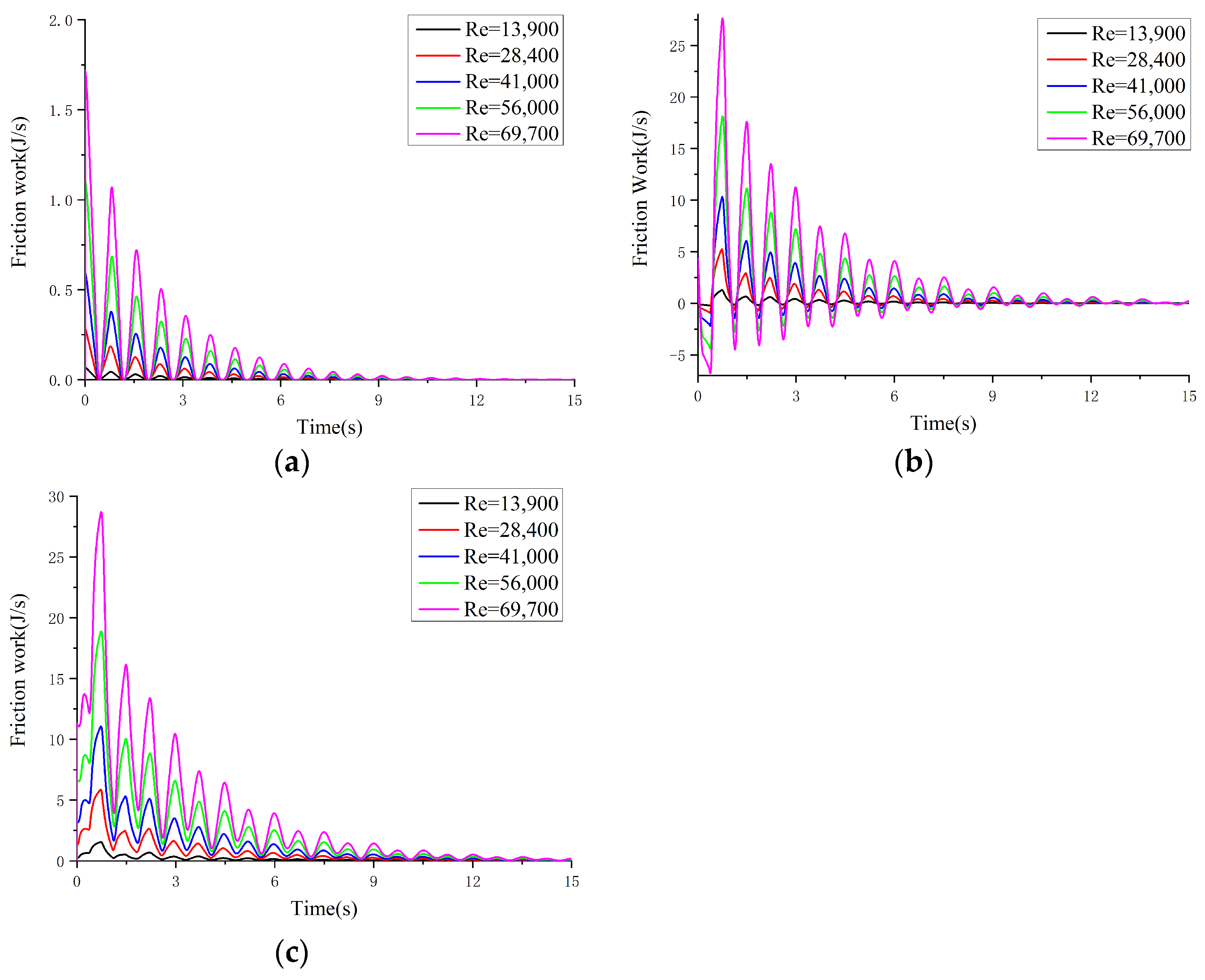
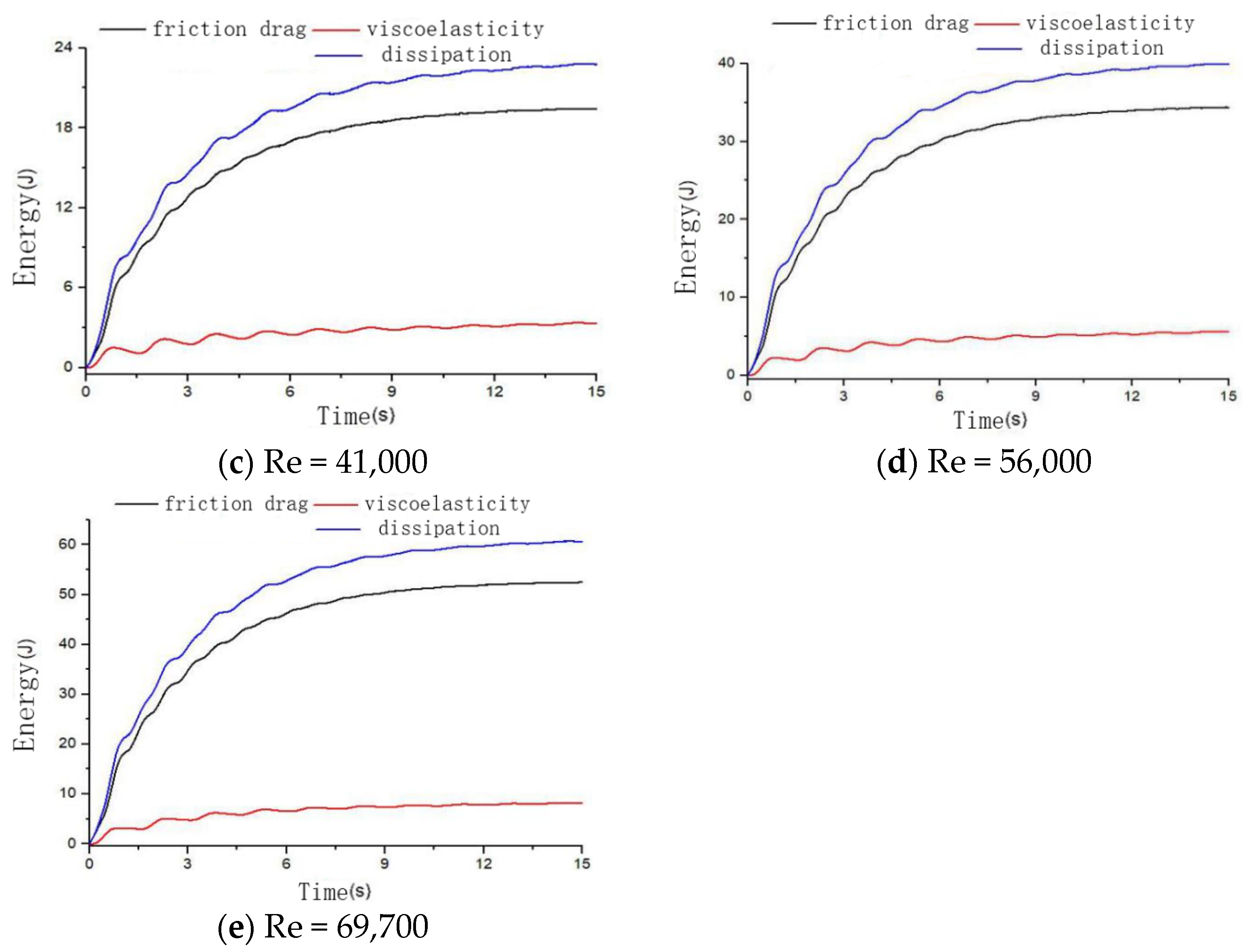
3.2.2. Performance of Friction Models under Different Reynolds Numbers

A one-dimensional steady friction model, a one-dimensional unsteady friction model, and a quasi-two-dimensional friction model were selected to investigate the performance of each friction model under different Re conditions. Figure 6 display the work curves for each model. The results show that the work performed by friction varied among different models.

From the perspective of frictional work, the one-dimensional steady-state model exhibited the lowest work values across various Re. The one-dimensional unsteady model displayed a large vibration amplitude with the peak values near those of the quasi-2D model and similar fluctuation frequency. However, its valley values were lower and sometimes negative, unlike the other two models.

In addition, the results of transient flow energy dissipation in the different friction models under the condition of specific Reynolds number Re = 28,400 are shown in Figure 7.

Next, we analyzed the impact of friction on transient flow energy dissipation under different friction models. Figure 8 showcases the results for various Re conditions.

As observed in Figure 8, the one-dimensional steady-state friction model exhibited the least energy loss compared with other models. The energy dissipation generated by the quasi-2D and one-dimensional unsteady models differed considerably. Notably, the quasi-2D model consistently displayed approximately two-fold friction energy dissipation compared to the one-dimensional unsteady model across various Re conditions (as shown in the Supplementary Materials). Selecting an appropriate friction model is crucial for accurately analyzing the impact of transient flow pressure wave energy in viscoelastic pipelines.

3.3. Selecting the Optimal Friction Model

While various frictional models impact energy dissipation (Section 3.2), further analysis is necessary to determine the optimal model for studying transient flows according to both friction and viscoelastic effects. The pressure simulation results of the quasi-two-dimensional friction model coincide most closely with the experimental data in Figure 3, as shown in Figure 9a. To further investigate the model performance, the numerical simulation results of the three friction models were compared. Figure 9b displays the pressure fluctuations obtained with each model (a single plot for the representative Re is shown, with additional comparisons at other Re conditions placed in the Supplementary Materials).

The simulation results of pressure with the quasi-two-dimensional friction model coincide most closely with the experimental data obtained by the laboratory bench shown in Figure 3, and the comparison results are shown in Figure 9a. The two models are similar to the experimental data at the initial peak value, but the data of the quasi-two-dimensional model are much closer to the experimental data over time. The simulation results of the two models are close to the experimental results in the initial peak, but with the passage of time, the simulation results of the quasi-two-dimensional model are closer and more consistent with the experimental results, which can be clearly observed in the figure. The one-dimensional steady-state model exhibited higher amplitude and shorter time intervals between peaks compared to the one-dimensional unsteady model, leading to higher vibration frequency.

While both one-dimensional frictional models approached the quasi-2D model’s peak pressure, they showed larger subsequent pressure fluctuations. The peak pressure was higher than the quasi-2D model pressure, and the valley pressure was lower than the quasi-2D model pressure, indicating that the vibration amplitude of the quasi-two-dimensional model was the smallest among the three models. Simultaneously, with time, the vibration frequency of the one-dimensional model turned higher than that of the quasi-two-dimensional model; that is, the time of extreme pressure was earlier than that of the quasi-two model. Figure 9b highlights the close agreement between the quasi-two-dimensional and one-dimensional unsteady models at a specific Re, while the one-dimensional steady-state model exhibits the largest deviation from the quasi-2D model. Taking these observations into account, the quasi-two-dimensional friction model emerges as the optimal choice for analyzing transient flows in viscoelastic pipelines. This preference is justified by its superior alignment with the experimental data and its capability to capture the essential characteristics of the pressure fluctuations, including vibration amplitude and peak pressure timing. Compared with the one-dimensional steady-state friction model or one-dimensional unsteady friction model, the quasi-two-dimensional transient flow model possesses obvious advantages in terms of maximum pressure, peak pressure, trough pressure, and pressure wave period, and it has better follow ability with experimental pressure, which greatly improves the fitting accuracy of transient flow. At the pressure valley value, the simulated pressure of the quasi-two-dimensional friction model is much higher than that of the one-dimensional model, which is close to the experimental value, and it can reflect the actual situation well. In addition, the pressure wave period of the quasi-two-dimensional model is consistent with that of the experimental pressure wave, and the time difference is small and can be ignored. In the following paper, the quasi-two-dimensional transient flow model of a viscoelastic pipeline will be used for analysis and calculation.

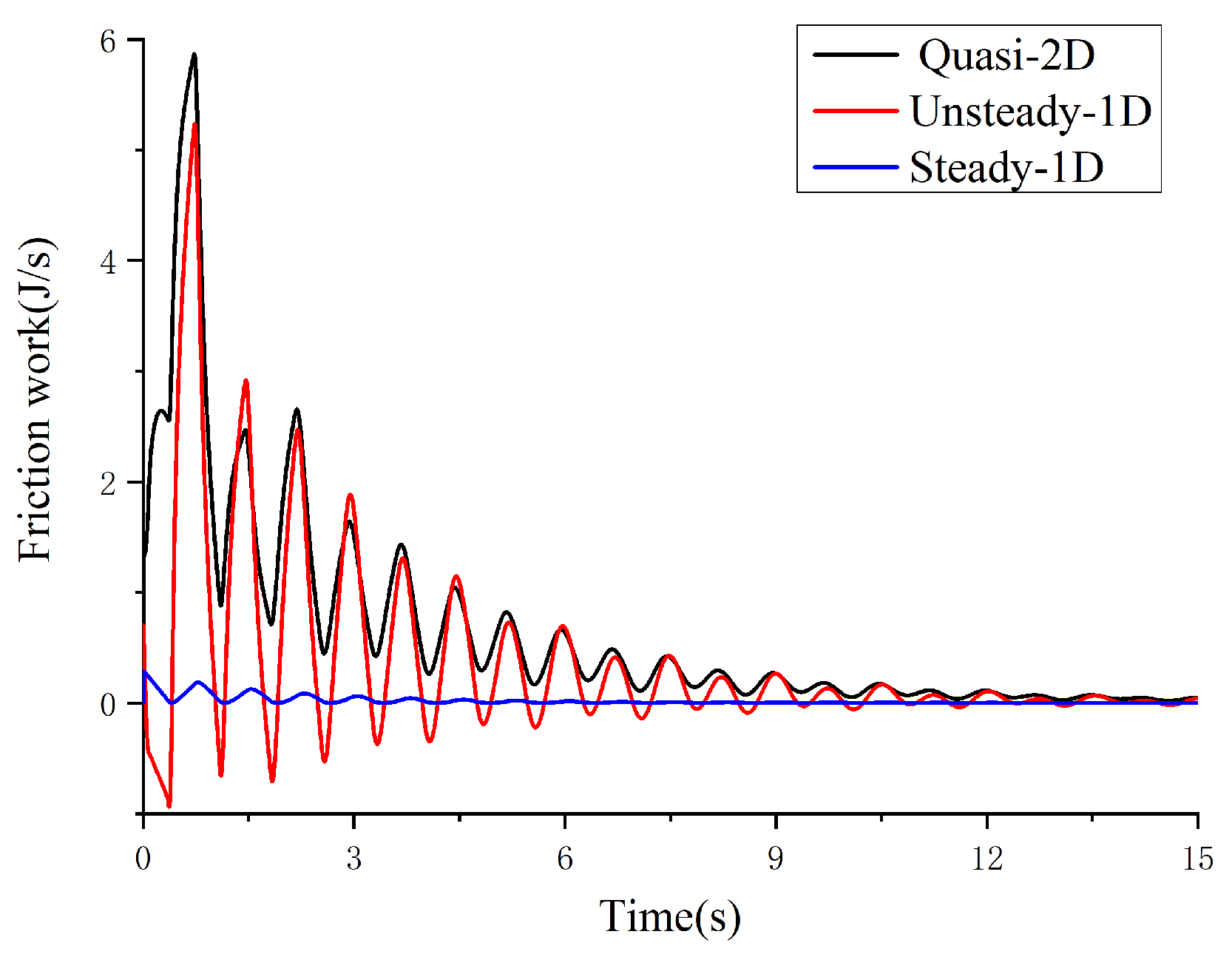
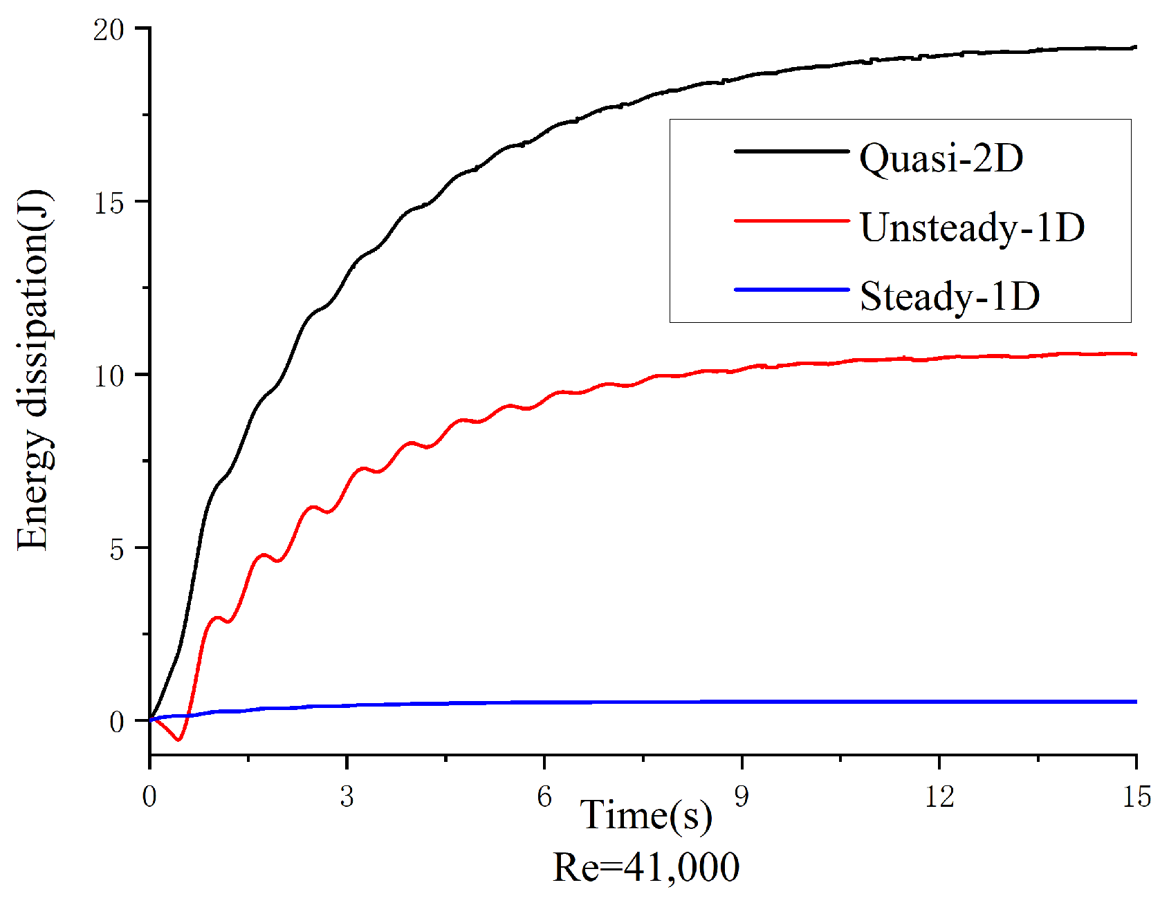
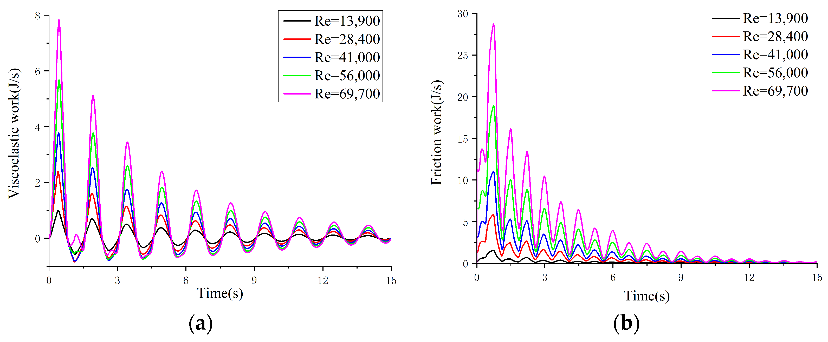
3.4. Quasi-Two-Dimensional Model and Viscoelastic Work

The transient flow pressure wave attenuation has a great relationship with the friction model, which was determined to be a more accurate friction model in Section 3.2. In addition to the constitutive characteristics of pipeline materials and the friction model, and considering that the interaction between fluid and pipeline will have a certain impact on the propagation of transient flow pressure waves, the flow state of the fluid in the pipe may also have a considerable impact. Thus, the impact of transient flow pressure wave attenuation under different Reynolds number conditions is studied in the following section.

Having established the quasi-2D model’s superiority in capturing transient flow behavior, we sought to explore its further application by investigating the combined influence of the quasi-two-dimensional model and viscoelastic properties on transient flow fluctuations with different Re conditions.

The results of the friction work, viscoelastic work, and energy dissipation based on the energy analysis method are shown in Figure 10.

The work performed by the friction resistance between the fluid near the wall and the pipe wall simulated by the quasi-2D model of the viscoelastic pipe was the same as that performed by the viscoelastic pipe on the order of magnitude, and both showed periodic fluctuations (Figure 10). Moreover, the work performed by the frictional resistance near the wall was greater than that of the viscoelastic resistance, indicating that the energy dissipation caused by the frictional resistance played a major role in the total energy of the transient flow in the viscoelastic pipe.

Figure 11 presents the results across a wider range of Re values, indicating the interplay between frictional work and viscoelastic behavior under varying Reynolds condition.

Both the frictional and viscoelastic works increased with the Re, as shown in Figure 11. Furthermore, Figure 11 shows that with an increase in the Re, the peak value of the energy loss caused by the frictional resistance of the viscoelastic pipelines continued to increase. Under different Re conditions, the energy loss caused by the viscoelastic pipelines was smaller than that caused by frictional resistance, and the proportion of energy loss generated by the two pipelines did not change significantly with an increase in the Re.

Moreover, the frictional dissipation caused by the frictional resistance model was much larger than that caused by the viscoelastic pipe in terms of energy dissipation, as shown in Figure 11. The constitutive characteristics of a viscoelastic pipeline under the excitation of a transient flow play a major role in energy absorption, showing an evident fluid–structure coupling effect. This energy primarily contributed the pipe material’s fatigue of the viscoelasticity, and the friction work caused by the viscoelastic pipe was significantly smaller than the friction effect of the friction model. Therefore, further research and analysis are required to explore the selection of the frictional model and its influence, along with other pertinent factors, on both the frictional model and the viscoelastic loss of the pipeline. This necessitates a thorough examination tailored to specific situations.

4. Conclusions

This study investigated the influence of friction models and viscoelastic constitutive effects on pressure fluctuations in viscoelastic pipelines using an energy analysis approach. We found that compared with elastic pipelines, viscoelastic pipelines exhibited stronger pressure wave attenuation, while the maximum pressure peaks remained comparable. However, the attenuation behavior became increasingly different with increasing Re, highlighting the need to consider viscoelastic effects beyond the peak pressure estimation. Moreover, different friction models significantly impacted the analysis, with the quasi-two-dimensional model demonstrating the best agreement with experimental data and consistent energy dissipation behavior. Finally, frictional work dominated the total energy dissipation during transient flow, while the viscoelastic material primarily absorbed energy for deformation and fatigue, contributing to wave attenuation. Therefore, for accurate analysis of pressure fluctuations in viscoelastic pipelines, careful selection of both the friction model and the approach to account for viscoelastic effects is crucial. Further exploration is warranted in the study of transient flow in viscoelastic pipes, particularly from perspectives such as temperature and other variables to delve deeper into their hydraulic behavior and governing principles. The insights drawn from this paper will be instrumental in elucidating the hydraulic principles governing transient flow in viscoelastic pipelines, enhancing the operational safety of water conveyance systems, and advancing the methodologies for monitoring leakage points through pressure wave analysis.

References

1. Lupa, S.I.; Gagnon, M.; Muntean, S.; Abdul-Nour, G. The impact of water hammer on hydraulic power units. Energies 2022, 15, 1526. [Google Scholar] [CrossRef]
2. Alabtah, F.G.; Mahdi, E.; Eliyan, F.F. The use of fiber reinforced polymeric composites in pipelines: A review. Compos. Struct. 2021, 276, 114595. [Google Scholar] [CrossRef]
3. Sun, Q.; Wang, F.X.; Wu, Y.B.; Xu, Y.; Hao, Y.Q. Energy analysis of transient flow with cavitation by considering the effect of water temperature in viscoelastic pipes. J. Hydroinformatics 2023, 25, 2034–2052. [Google Scholar] [CrossRef]
4. Andrade, D.M.; Rachid, F.B.D.; Tijsseling, A.S. Fluid transients in viscoelastic pipes via an internal variable con-stitutive theory. Appl. Math. Model. 2023, 114, 846–869. [Google Scholar] [CrossRef]
5. Gally, M.; Güney, M.; Rieutord, E. Investigation of pressure transients in viscoelastic pipes. J. Fluids Eng. 1979, 101, 495–499. [Google Scholar] [CrossRef]
6. Mousavifard, M.; Norooz, R. Numerical analysis of transient cavitating pipe flow by Quasi 2D and 1D models. J. Hydraul. Res. 2022, 60, 295–310. [Google Scholar] [CrossRef]
7. Wylie, E.B.; Streeter, V.L.; Suo, L. Fluid Transients in Systems; Prentice Hall: Englewood Cliffs, NJ, USA, 1993. [Google Scholar]
8. Chen, M.; Pu, J. Practical calculation method for friction loss transient flow in long distance pipelines. Oil Gas Storage Transp. 2008, 27, 17–21. [Google Scholar] [CrossRef]
9. Liu, G.; Pu, J. Effect of transient current friction calculation and friction on hydraulic transients. Mech. Pract. 2003, 25, 3. [Google Scholar] [CrossRef]
10. Brunone, B.; Golia, U.M.; Greco, M. Some Remarks on the Momentum Equation for Fast Transients. In Proceedings of the International Meeting on Hydraulic Transients with Water Column Separation (9th Round Table of the IAHR Group), Valencia, Spain, 4–6 September 1991; pp. 201–209. Available online: https://www.mendeley.com/catalogue/c6168492-8039-3fc8-a17f-7dda88d77736/ (accessed on 8 April 2024).
11. Daily, W.L.; Hankey, W.L., Jr.; Olive, R.W.; Jordaan, J.M., Jr. Resistance coefficients for accelerated and decelerated flows through smooth tubes and orifices. Trans. ASME 1956, 78, 1071–1077. [Google Scholar] [CrossRef]
12. Guo, X.; Gao, Y. Nonconstant friction model of transient flow in pipeline leakage detection. J. Hydroelectr. Power Gener. 2008, 27, 42–47. (In Chinese) [Google Scholar]
13. Ohmi, M.; Kyomen, S.; Usui, T. Numerical analysis of transient turbulent flow in a liquid line. Bull. Jpn. Soc. Mech. Eng. 1985, 28, 799–806. [Google Scholar] [CrossRef]
14. Vardy, A.E.; Hwang, K. A characteristics model of transient friction in pipes. J. Hydraul. Res. 1991, 29, 669–684. [Google Scholar] [CrossRef]
15. Duan, H.F.; Ghidaoui, M.S.; Lee, P.J.; Tung, Y.K. Unsteady friction viscoelasticity in pipe fluid transients. J. Hydraul. Res. 2010, 48, 354–362. [Google Scholar] [CrossRef]
16. Pezzinga, G.; Brunone, B.; Meniconi, S. Relevance of pipe period on Kelvin-Voigt viscoelastic parameters: 1D and 2D inverse transient analysis. J. Hydraul. Eng. 2016, 142, 04016063. [Google Scholar] [CrossRef]
17. Wahba, E.M. On the two-dimensional characteristics of laminar fluid transients in viscoelastic pipes. J. Fluids Struct. 2017, 68, 113–124. [Google Scholar] [CrossRef]
18. Meniconi, S.; Duan, F.H.; Brunone, B.; Ghidaoui, M.S.; Lee, P.J.; Ferrante, M. Further developments in rapidly decelerating turbulent pipe flow modeling. J. Hydraul. Eng. 2014, 140, 04014028. [Google Scholar] [CrossRef]
19. Duan, H.F.; Ghidaoui, M.S.; Tung, Y.K. Energy analysis of viscoelasticity effect in pipe fluid transients. J. Appl. Mech. 2010, 77, 044503. [Google Scholar] [CrossRef]
20. Duan, H.F.; Meniconi, S.; Lee, P.J.; Brunone, B.; Ghidaoui, M.S. Local and integral energy-based evaluation for the unsteady friction relevance in transient pipe flows. J. Hydraul. Eng. 2017, 143, 04017015. [Google Scholar] [CrossRef]
21. Wu, K.; Feng, Y.; Xu, Y.; Liang, H.; Liu, G. Energy Analysis of a quasi-two-dimensional friction model for simulation of transient flows in viscoelastic pipes. Water 2022, 14, 3258. [Google Scholar] [CrossRef]
22. Yu, H.; Li, F.; Yang, H.; Zhang, L. Nonlinear high elastic-viscoelastic constitutive model of rubber materials under finite deformation. Rubber Ind. 2017, 64, 645–649. [Google Scholar] [CrossRef]
23. Keramat, A.; Kolahi, A.G.; Ahmadi, A. Water hammer modelling of viscoelastic pipes with a time-dependent Poisson’s ratio. J. Fluids Struct. 2013, 43, 164–178. [Google Scholar] [CrossRef]
24. Bradford, S.F. Development of a Godunov-type model for the accurate simulation of dispersion dominated waves. Ocean Model. 2016, 106, 58–67. [Google Scholar] [CrossRef]
Figure 1. Generalized Kelvin–Voigt model.(ηi is the ith model).
Water 16 01468 g001
Figure 2. Plan of the physical model experiment. Here, T represents the supply tank, DM represents the discharge measurement section, MS represents the pressure measurement section, and MV represents the maneuver valve.
Water 16 01468 g002
Figure 3. Schematic of the test platform.
Water 16 01468 g003
Figure 4. Transient flow pressure in viscoelastic pipes: (a) elastic pipes (b) with different Reynolds numbers (Re).
Water 16 01468 g004
Figure 5. Comparison of transient flow pressures in viscoelastic and elastic pipes under different Reynolds number conditions (Re = 41,000; others in the Supplementary Materials).
Water 16 01468 g005
Figure 6. Work performed by different friction models at various Reynolds numbers. (a) One-dimensional steady-state friction model. (b) One-dimensional unsteady friction model. (c) Quasi-two-dimensional friction model.
Water 16 01468 g006
Figure 7. Work comparison for different motorcycle group models (Re = 28,400).
Water 16 01468 g007
Figure 8. Dissipative energy comparison for different transient flow models (Re = 41,000; others in the Supplementary Materials).
Water 16 01468 g008
Figure 9. (a) Transient pressure fluctuation at the pressure measurement point (25 °C). (b) Comparison of pressure simulation results for different friction models (Re = 41,000; others in the Supplementary Materials).
Water 16 01468 g009
Figure 10. Comparison of total dissipation (dissipation), frictional dissipation, and viscoelastic dissipation of quasi-two-dimensional transient flow models in viscoelastic pipes under different Reynolds numbers. (Re = 13,900, 28,400, 41,000, 56,000, 69,700) (Dissipation is at the top; viscoelasticity is at the bottom).
Water 16 01468 g010aWater 16 01468 g010b
Figure 11. Work variation in the quasi-2D transient flow model. Energy change due to (a) viscoelasticity and (b) friction pipe work.
Water 16 01468 g011