Article

Comparing Four Evapotranspiration Partitioning Methods from Eddy Covariance Considering Turbulent Mixing in a Poplar Plantation

1
Research Institute of Forestry, Chinese Academy of Forestry, Beijing 100091, China
2
Collaborative Innovation Center of Sustainable Forestry in Southern China, Nanjing Forest University, Nanjing 210037, China
3
Henan Xiaolangdi Forest Ecosystem National Observation and Research Station, Jiyuan 454650, China
4
Jining Polytechnic, Jining 272000, China
*
Authors to whom correspondence should be addressed.
Water 2024, 16(11), 1548; https://doi.org/10.3390/w16111548
Submission received: 17 April 2024 / Revised: 20 May 2024 / Accepted: 22 May 2024 / Published: 28 May 2024
(This article belongs to the Section Ecohydrology)

Abstract

:
Evapotranspiration is a key link in the water cycle of terrestrial ecosystems, and the partitioning of evapotranspiration is a prerequisite for diagnosing vegetation growth and water use strategies. In this study, we used double-layer eddy covariance (DLEC) measurements within and above the canopy of poplar plantations to divide evapotranspiration into transpiration and evaporation during the growing season. We diagnosed the coupling state of airflows in the canopy vertical layer and found that the daytime coupling state at the half-hourly scale can mask nighttime decoupling. Furthermore, we investigated the daytime and nighttime vertical layer airflow coupling states separately and quantified the effects of coupling states on the DLEC of resolved transpiration. The partitioning results of the DLEC method were taken as the standard after the airflow coupling test. Then, the performance and accuracy of evapotranspiration partitioning for the modified relaxed eddy accumulation (MREA), the conditional eddy covariance (CEC), and the flux variance similarity (FVS) with DLEC were compared. Transpiration calculated from MREA showed the best agreement with DLEC, and the other methods showed different degrees of underestimation (1:1 slope = 0.64–0.83). Evaporation calculated from FVS showed the best agreement with DLEC, while CEC and FVS made an overestimation of more than 26% (1:1 slope = 1.26–1.99), but MREA made an underestimation from 5% to 35% (1:1 slope = 0.65–0.95). The correlation coefficients between DLEC and MREA for transpiration were 0.95–0.97 with RMSEs of 15.52–17.04 W m−2, and those between DLEC and FVS for transpiration were 0.73–0.78 with RMSEs of 10–21.26 W m−2 at the daily half-hourly scale. A detailed comparison of the differences between DLEC and evapotranspiration partitioning methods from high-frequency eddy covariance data under the condition of canopy vertical layer airflow mixing provides knowledge about the consistency of results for evapotranspiration partitioning in poplar plantation forests.

1. Introduction

Evapotranspiration is a key component of the water cycle and energy balance in terrestrial ecosystems and can be classified according to its components as ecosystem transpiration related to plant stomata and ecosystem evaporation of nonstomatal components, and the latter specifically includes surface evaporation components such as foliar evaporation and soil evaporation [1]. Transpiration and evaporation can effectively reduce the surface temperature, relieving the greenhouse effect. However, the fertilization effect of rising CO2 concentrations [2] accelerates plant growth, leading to higher water use efficiency and relatively lower transpiration rates [3,4], which in turn lead to global warming and drying [5] and an increase in surface temperature. The feedback relationship between evapotranspiration components and the environment is complex, and the precise partitioning of evapotranspiration components is important for thoroughly elucidating the feedback processes and roles between components and the environment.
Considering that the water coupled carbon relationship model based on flux observation is a better starting point from which to investigate the partitioning of ecosystem evapotranspiration components, some new separation methods have been developed in recent years based on this assumption: Zhou et al. proposed potential water use efficiency and apparent water use efficiency using ET and GPP from flux observation sites under the premise of satisfying three assumptions of evapotranspiration partitioning [6]. Scott and Biederman used a statistically significant positive intercept (soil evaporation term) in the model to achieve T/ET estimation [7]. Only continuous flux observations over relatively long periods (at least three years) can guarantee the physical significance of the intercept term. Nelson et al. estimated the temporal pattern of WUE using total primary productivity and evapotranspiration by separating the period in which transpiration dominates and using a random forest approach to train the WUE within the period in each short time interval to achieve partitioning of evapotranspiration [8]. Although the TEA algorithm output is robust to dataset noise, it exhibits some sensitivity to sites and model structures where evapotranspiration is relatively constant, leading to ecosystem evapotranspiration overestimation.
In terms of practical observations that can evade the disadvantages of these models with a lack of independent universal validation of evapotranspiration components and their assumptions, the direct separation of ecosystem-scale evapotranspiration into transpiration and soil evaporation is still extremely challenging [9].
Methods to separate evapotranspiration based on observational perspectives include (1) the sap flow method (SF) or the micro-lysimeter (ML) method combined with flux observations; (2) isotope observations; and (3) high-frequency eddy covariance observation [10]. The sap flow method has major advantages for single-tree transpiration measurements but still suffers from coefficient correction, thermal damage, and scale expansion [11,12], which introduce some errors in the estimation of transpiration. The micro-lysimeter method allows direct measurement of soil evaporation at the site [13], and is used for validation of soil evaporation models [14]. Eddy covariance observation is a well-recognized method for studying water–carbon fluxes in ecosystems and has been used worldwide. The direct partitioning of evapotranspiration from eddy covariance observations consists of three main types of methods: the modified relaxed eddy accumulation (MREA) method [15,16,17], the conditional eddy covariance (CEC) method [17], and the flux variance similarity (FVS) method [18,19]. The relaxed eddy accumulation method considered only the nonstomatal process fluxes and solved for the stomatal component fluxes as a residual term, which resulted in an overestimation of transpiration [16,17]. The conditional eddy covariance method considered both stomatal and nonstomatal processes in the effective jet information and extended it to half-hourly flux results for evapotranspiration components [17]. The flux variance similarity approach is based on the processes of stomatal and nonstomatal components at the same time and applies the flux variance similarity principle to each process, resolving the correlation coefficients of the respective components between water and carbon fluctuations with the estimation of leaf-scale water use efficiency to achieve direct partitioning for ecosystem transpiration and soil evaporation [18,19].
The double-layer eddy covariance method simultaneously observes the turbulent exchange within and above the canopy; it is used to explain or complement the contribution of understory vegetation and soil in energy fluxes or carbon fluxes to the fluxes above the canopy. In the study of the carbon dioxide balance of forest ecosystems, this method is used to investigate the effect of subcanopy decoupling or advection on the above-canopy carbon dioxide exchange and to further correct the carbon balance of forest ecosystems under decoupling conditions [20,21]. However, relatively few studies have focused on how to effectively separate ecosystem evapotranspiration components by using the double-layer eddy covariance method [9,12,22].
Recently, Paul-Limoges et al. improved on the known limitations of this method and developed systematic treatments to achieve the goal of partitioning evapotranspiration in forest ecosystems by simultaneously using EC measurements below and above the canopy [9]. The DLEC method has encountered more limitations in its subsequent use, including the test and delineation of coupling between layers [23] and inverse gradient transport of eddies within the canopy [24]. The most important is the coupling state of airflows crossing the canopy vertical layer. The effect of different coupling states on the application of the DLEC method to separate evapotranspiration is unknown for specific sites, so it is necessary to delineate and interpret the coupling states of air masses below and above the canopy for specific flux sites, especially in the study of carbon balance and evapotranspiration separation in forest ecosystems [20,21,23,25]. The diagnosis of the coupling state ensures an effective understanding of the mixing of the vertical-layer gas masses [26], further helping to determine the best decoupling index for comparison with the performance of the CEC, FVS, and MREA methods for separating evapotranspiration when full coupling conditions are met.
In this study, our objectives are (1) to investigate state of turbulence coupling using EC measurements within and above the poplar plantation canopy; (2) to apply different approaches to determine coupling and decoupling in the Poplar plantation and further partition E and T from ET accordingly; and (3) to access the performance and accuracy of evapotranspiration partitioning based on the CEC method, FVS method and MREA method consistently under turbulence coupling conditions.

2. Materials and Methods

2.1. The Site Introduction

The observation experiment was carried out at the MinQuan site (MQ site) at Henan-Huaihai Farmland Protection Forest Ecosystem Positioning Observation (115°05′42″ E, 34°43′22″ N, mean elevation 102 m). The study site is located in Minquan County, Henan Province, which has a warm temperate monsoon climate with southeast winds prevailing during the growing season. The average multiyear temperature is 14.4 °C, the average multiyear precipitation is 678 mm, and the seasonal distribution of precipitation is uneven. The main tree species is poplar (Populus nigra L.), with an age of 20a and an average canopy height of 17 m, and there are no shrubs under poplar trees. Herbaceous plants mainly include Senna tora (L.) Roxb., Setaria viridis (Linn.) Beauv, and Rifolium incarnatum Linn., with a total cover of 31%. The leaf area index (LAI) during the study period was 2.6 to 2.8, the plant spacing was 6 m × 6.5 m, the height under live branches was 4 m, the canopy closure was 0.51, and the soil was sandy loam.
The two eddy covariance systems at the MQ site were uniformly installed southeast of the observation tower at heights of 24 m and 2 m. Each EC system consisted of a sonic anemometer thermometer (CSAT3, Campbell Scientific, Logan, UT, USA) and an open-path infrared gas analyzer (LI7500, Lincoln, NE, USA). Raw data were collected by a logger (CR1000, Campbell Scientific, Logan, UT, USA) with a sampling frequency of 10 Hz. The micrometeorological observation gradient system consisted of four layers of air temperature and humidity sensors installed at 9 m, 17 m, 20 m, and 32 m. Total radiation (SP Lite2, Kipp & Zonen, Delft, The Netherlands) and net radiation (NP Lite2, Delft, The Netherlands) were also installed at a height of 32 m. A rain gauge (TE525MM, Campbell Scientific, Logan, UT, USA) was installed at 2 m and 32 m. The above instruments were connected to a data logger (CR1000X, Campbell Scientific, Logan, UT, USA) with a scanning frequency of 15 s and a set of data outputs every 30 min.

2.2. Evapotranspiration Partitioning and Data Processing

2.2.1. The Double-Layer Eddy Covariance (DLEC) Method

Double-layer eddy covariance (DLEC) measurements require the installation of EC systems at two height positions above and below the canopy to separate ecosystem evapotranspiration. Total ecosystem evapotranspiration observed above the canopy includes plant transpiration, canopy evaporation, and soil evaporation by source, while total understory evapotranspiration observed below the canopy includes transpiration from understory groundcover plants and soil evaporation [9]. Thus, for forest ecosystems with negligible canopy evaporation, ecosystem evapotranspiration approximates arboreal evapotranspiration at low E/ET, which can be derived using double-layer eddy correlation observations with the following equation:
T R = E T a b o v e E T b e l o w
Before the separation process, it is necessary to exclude data for all periods with precipitation > 0.1 mm to exclude data with negative water vapor flux and subcanopy air temperature above the dew point temperature [9], most importantly, to determine the state of canopy vertical layer air mass coupling and the best diagnostic index for a specific site.
Here, we choose several indicators to test the coupling state of airflow, including the friction velocity (u*) [27], the mean wind speed (U) [28], the standard deviation of vertical wind speed (σw) [29], and the integral turbulence characteristics σw/u* and σw/U [30,31]. We used all the half-hour data of σw to determine the airflow coupling state qualitatively, and then the airflow coupling threshold was quantitatively analyzed by dividing the interval. We also investigated the airflow coupling between the canopy and atmosphere in detail. After finishing this process, we obtained the best indicator for our site and used it to ensure that airflow coupling occurred throughout the day to partition evapotranspiration.

2.2.2. The Determination of the Coupling State across the Canopy Vertical Layer

The state of interlayer coupling determines the representativeness of EC measurements above the canopy and determines whether coupling is significant for studying carbon balance and the separation of evapotranspiration in forest ecosystems. Referring to the vertical-layer air mass coupling indicators used by previous authors to investigate ecosystem carbon balance and carbon balance [23,32,33], considering that the difference in the coupling state determined by different methods at this site will introduce some error in the evapotranspiration separation, different threshold diagnostics are used for the following scenarios: (1) the interlayer airflow is fully coupled, (2) the interlayer airflow is fully coupled during the day and decoupled during the night and (3) even during the day when turbulence exchange is more adequate, and (3) it is assumed that even in the daytime when the turbulence exchange is more adequate, there is still a certain degree of decoupling and a more serious decoupling at night. In forest ecosystems with open canopies, the three scenarios correspond to increasing stringency of the criteria for judging airflow coupling above the canopy–subcanopy. The corresponding indices for judging the degree of coupling in this study for the three scenarios correspond to (1) conventional above-canopy u* = 0.20 m s−1; (2) a single-level u* threshold of 0.2 m s−1,, a single-level vertical wind speed standard deviation threshold of 0.21 m s−1, a dual-level nighttime u* of (0.32, 0.048), and a dual-level nighttime vertical wind speed standard deviation of (0.359, 0.063); and (3) the relationship of daytime vertical wind speed standard deviation is considered separately, and the final threshold is obtained as (0.165, 0.0558); the threshold value is (0.136, 0.0524) considering the double-level u* to judge the coupling state. The data were screened and controlled using the above three scenarios, and the details of the valid data obtained are shown in Table 1.
From Table 1, the proportion of total valid data decreases with the stringency of the coupling state, regardless of whether single- or dual-level threshold diagnostic metrics are used, with 57.94% of the total valid data for the fully coupled state, 43–48% of the total valid data considering only the nighttime uncoupled state, and 32–41% of the total valid data considering the daytime decoupling. This result is consistent with our expectations.
The diagnostic thresholds for the three coupled states consider the vertical mixing of air masses and data quality and missing issues, and it is considered appropriate not to use a single mixing indicator for an accurate description of this site but to choose a combination of single mixing indicators for further analysis. That is, considering the uncertainties and errors brought by the coupling states on evapotranspiration separation, we analyzed the effects of different coupling states of the open plantation canopy on ecosystem evapotranspiration measurements using methods 1.2, 2.2.2, and 3.2.2.

3. Results and Discussion

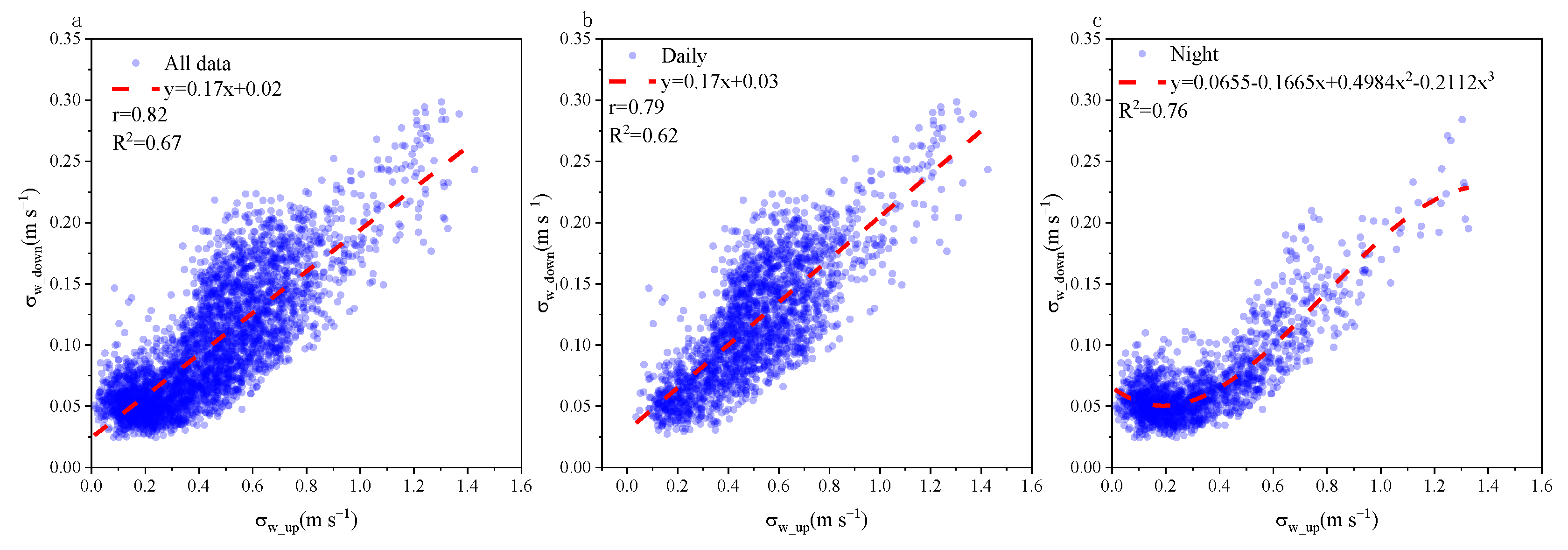
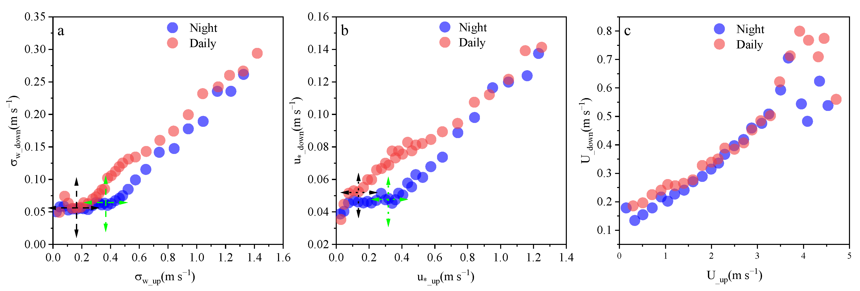
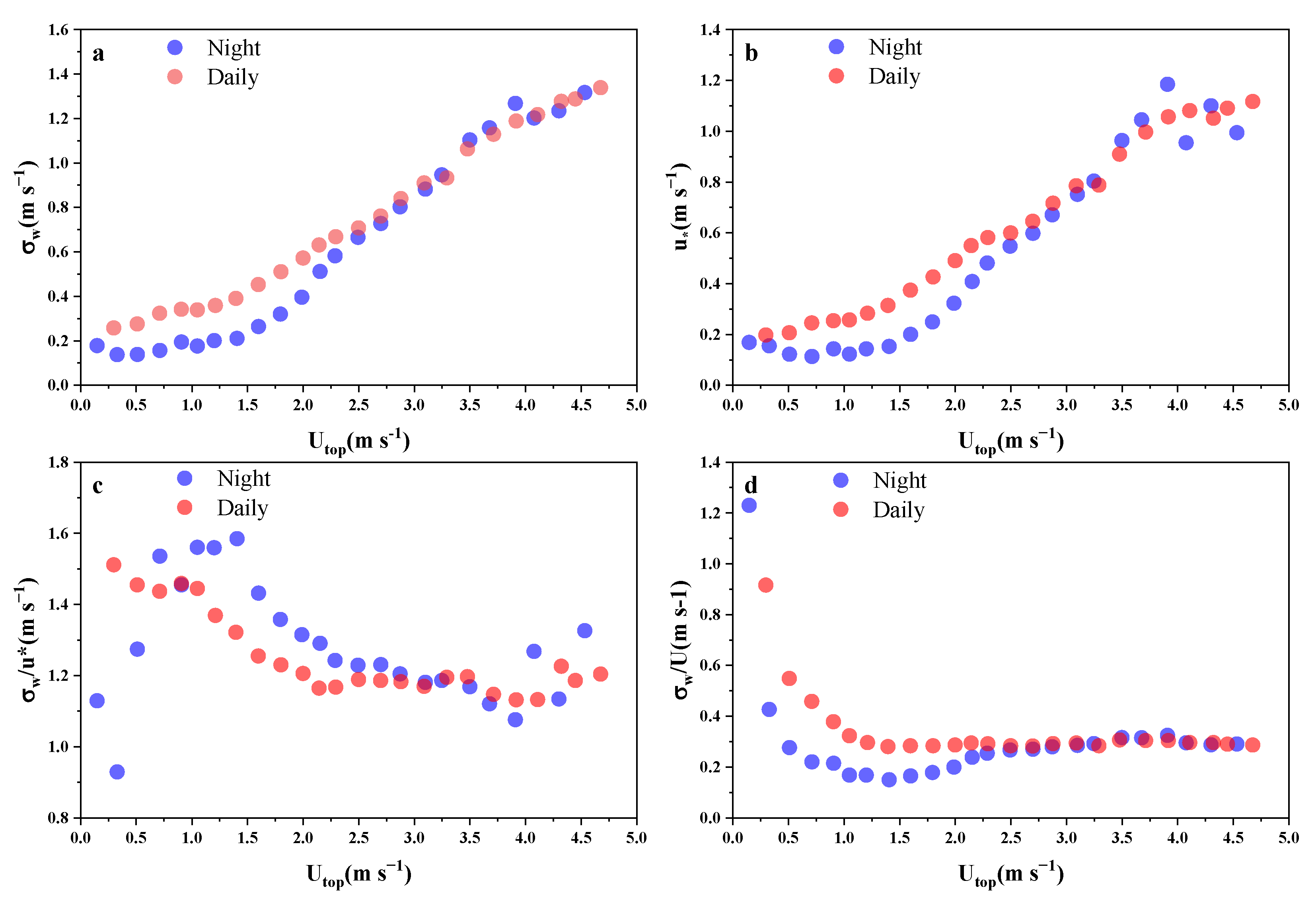
3.1. Coupling State of Airflow Crossing the Vertical Layer of the Plantation Canopy

The ideal for ecosystem flux observations is that turbulence occurring in all canopy–subcanopy–soil profile can be adequately mixed or exchanged and that EC observations can accurately capture turbulence information and flux contributions to ensure that fluxes calculated using simplified mass balance methods are representative of the entire ecosystem [34]. Thus, the substratum selection for sites in the flux network is mostly low or open vegetation (e.g., grasslands, scrub, agricultural fields, and forests), and this characteristic of the substratum often allows for adequate mixing of sources and sinks of scalar fluxes in the vertical layer. The mixing intensity of vertical-layer air masses is highly susceptible to canopy structure, including factors such as canopy cover, PAI, branch extension length, and trunk space [35]. The coupling state of the actual vertical layer can be theoretically classified into three major scenarios according to the coupling period: (1) fully coupled during both day and night; (2) coupled during the day and decoupled during the night; and (3) decoupled during both day and night. Considering the effect of tree space, we screened turbulence mixing indicators for the vertical layer of the incompletely covered plantation canopy. Excluding differences in the vertical exchange of day and night scalar turbulent fluxes, σw above the canopy was significantly linearly correlated with σw below the canopy (y = 0.17x + 0.02; R2 = 0.67), and forest sites with sparse canopies exhibit significant strong coupling behavior (Figure 1a). The main reason for this difference compared to the Thomas et al. study [23] is that the reduction in canopy depression leads to an increase in canopy vertical profile connectivity, which further enhances the proportion and depth of the canopy above which eddies can penetrate deeper into the subcanopy. Considering the different thermal and kinetic differences of the diurnal airflow, we distinguished between day and night to analyze the coupling state of the airflow in the vertical layer of the canopy. We found that σw above and below the canopy showed a significant linear correlation during daytime (y = 0.17x + 0.03, R2 = 0.62), while the nighttime showed a significant nonlinear relationship (y = 0.0655 − 0.1665x + 0.4984x2 − 0.2112x3, R2 = 0.76). In both cases, we seem to obtain a piece of knowledge about the coupled state artifact. Even for the sparse canopy, there is a clear decoupling phenomenon at night (Figure 1b,c), and the sparse canopy cannot be simply interpreted as fully coupled at the daily scale without any distinction because the daytime will confuse the decoupling phenomenon of the vertical layer at night. The cause of this state at night is mainly the subcanopy inversion process.
For undepressed stands, the standard deviation of frictional and vertical wind speeds above the canopy and in the subcanopy showed consistent characteristics of variation both during the day and at night. During the night, when the wind was weak, the subcanopy turbulence intensity was in an independent state from that above the canopy, but after the airflow above the canopy exceeded the thresholds of u* = 0.3 m s−1 and σw = 0.45 m s−1, respectively. The turbulence intensity above and below the canopy showed a linear relationship; even during the daytime when the wind was stronger, it showed the same behavior, with thresholds of u* = 0.3 m s−1 and σw = 0.4 m s−1 (slightly smaller) for the transition from the independent state to the linear relationship, respectively. The independence of the intensity of subcanopy turbulence from the intensity of overcanopy turbulence suggests either different independent mechanisms of turbulence action and disruption, that airflow is largely decoupled above and below the canopy, or that both play a role [23]. Subcanopy airflow at weak turbulence intensities exhibit convergence to a constant value behavior, and the sparse canopy structure preventing airflow from reaching the subcanopy deep inside the canopy does not seem to be the main reason for the independence of airflow above and below the canopy at the MQ site. In other words, overcanopy airflow and wind shear are the main sources of subcanopy turbulence. The subcanopy equivalent is greater during the day than at night for a given overcanopy turbulence intensity condition.
Wind shear similarly enhances the mixing of air masses between layers and further appears to increase the intensity of turbulence in the subcanopy layer under a weak overcanopy turbulence intensity. The wind speed above and below the canopy shows a consistent trend but tends to vary linearly above the canopy, while the subcanopy shows a nonlinear trend. An interesting phenomenon is that the air masses above and below the canopy rise staggeringly at wind speeds above the canopy of 2.3 m s−1 < Utop < 3.7 m s−1, while in the rest of the interval, the air masses are significantly stronger during the day than at night (Figure 2c).
For the airflow above the canopy, u* and σw show both similar variations and large differences for wind speed: after Utop > 1.5 m s−1, both show a strictly linear relationship; at Utop ≤ 1.5 m s−1, although both show an overall asymptotic behavior (turbulence intensity tends to a smaller constant value at Utop → 0), they show a weak daytime upward trend, and at night, they show a decrease followed by an increase (Figure 3). The strong linear relationship is explained by the fact that wind shear drives the turbulent exchange in the vertical layer, which enhances the interlayer coupling. The weak differences under low-wind-speed conditions can be explained by intense radiative heating during the daytime and wind shear at night. The σw/u* and σw/U both converge to constant values at high wind speed; the latter reaches the maximum under weak air mass flow conditions, while the former exhibits a haphazard and disordered behavior, which is mainly related to the irregular variation of u* under steady conditions, where shear, stress, etc., show significantly different directions [29].
We also examine the turbulent mixing state at the canopy–atmosphere interaction interface, and all of them show obvious decoupling–coupling–complete coupling behavior: the overall behavior shows a progressive distribution at low turbulence intensity above the canopy and gradually converges to a constant value; after reaching the turning point, both increase linearly with the increase in turbulence intensity above the canopy; the convergence behavior before the turning point shows decoupling behavior, and after crossing the decoupling–coupling threshold of the turbulence, a significant linear correlation is formed, which means that the gas masses above and below the canopy begin to couple; when the mixing intensity reaches a large enough level, a perfect correlation is shown between the gas masses above and below the canopy, indicating that the turbulence mixing in the whole vertical layer reaches the ideal state.

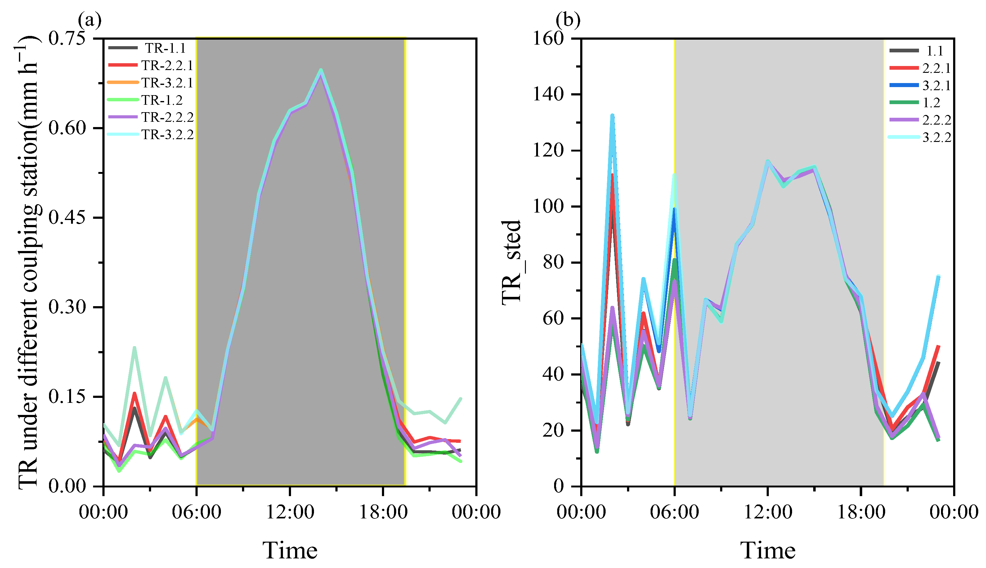
3.2. Do Different Coupling States Obviously Affect the Daily Transpiration in a Sparse Canopy?

The five threshold diagnostics corresponding to the three coupled states showed large differences in the daily variation in growing season evapotranspiration. In general, the more stringent the diagnosis of the inter-canopy airflow coupled state, the smaller its standard deviation, but the most stringent produced larger standard deviations due to the overly stringent threshold diagnostic process and the small amount of valid data (Table 1). Although we found the need for diurnal differentiation of thresholds at the half-hourly scale, for the separation of daytime evapotranspiration components in sparse ecosystems, 3.2.2 showed that the daytime canopy profile at the site was still considered to be dominated by the coupled state, as the diagnosis of the coupled state from 06:00 to 18:00 was found not to lead to significant differences in the inter-day variability of ecosystem evapotranspiration between the two coupled–decoupled states. This result is in agreement with the results of a study on carbon balance, which was mainly due to open canopy conditions and flat topography around EC towers [33]. On the other hand, the growing season ecosystem transpiration showed a clear daily variation characterized by a distinct single-peaked curve. This process is necessary for nighttime coupled state diagnosis, where different coupled states exhibit great variability; 3.2.2 exhibits large evapotranspiration values and standard deviations, and 2.2.2 threshold diagnostics have the smoothest variation in evapotranspiration and the smallest standard error, which can be used as a coupled diagnostic indicator for this site (Figure 4).

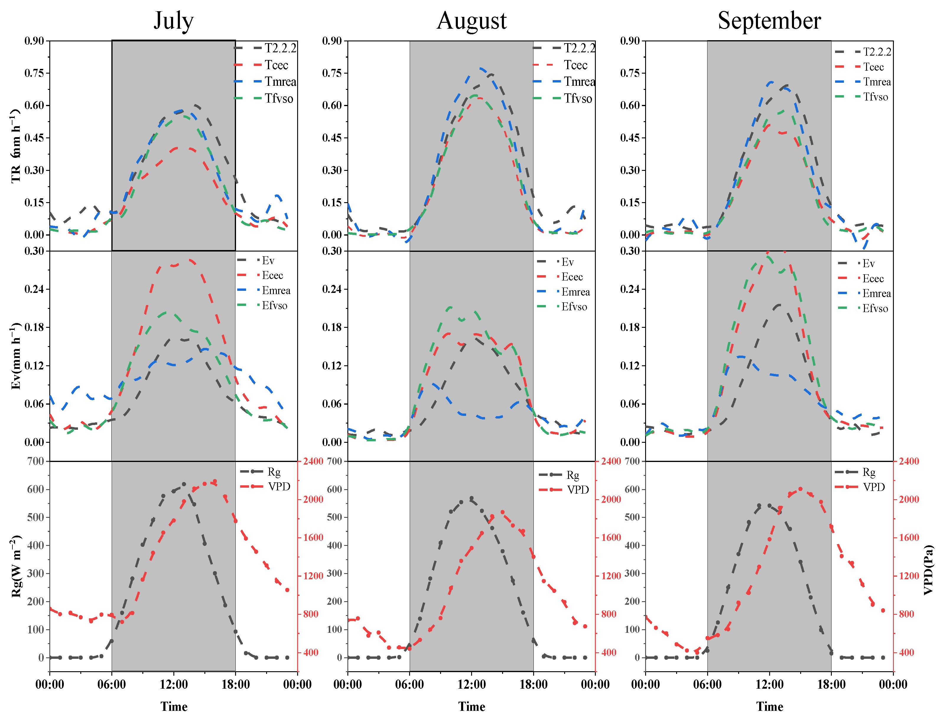
3.3. Comparison of the Results of Different Partitioning Methods

Through the analysis of the open canopy coupled state in Section 2.2.2, transpiration and soil evaporation were separated using the coupling threshold diagnosis method proposed in Appendix A with the CEC, MREA, and FVS methods. Under sparse canopy conditions, the DLEC method achieved a solution rate of 54.01% in the separation of evapotranspiration components, with 62.18%, 50.54%, and 49.45% in each month; the CEC method achieved a solution rate of 88.61% in the separation of evapotranspiration components, with 96.06%, 91.06%, and 78.62% in each month; the solution rate of the MREA method was 58.04% in the separation of evapotranspiration components, and the solution rates were 67.63%, 57.59%, and 48.90% in each month; the solution rate of the FVS method was 53.96% in the separation of evapotranspiration components, and the solution rates were 62.99%, 52.54%, and 48.36% in each month. Among the separation methods, the solution rates were CEC > MREA > DLEC = FVS. The CEC method showed higher solution rates for sparse canopy flux fraction separation, which is consistent with forest stand studies [17] on C3 crops with 31–39% separation success [36], and it can be seen that the FVS optimization algorithm has a higher percentage of successful separation under open canopy understory conditions (48–63%).
From July to September of the growing season, the total average daily growing season evapotranspiration based on the two-layer eddy correlation was 5.79 mm d−1 above the canopy and 1.53 mmd−1 in the subcanopy, with a T/ET of 79.02%; the monthly average ecosystem transpiration was 6.0, 6.06, and 5.31 mm d−1 above the canopy, and the soil evaporation was 1.63, 1.41, and 1.56 mm d−1 in the subcanopy, respectively (Table 2). T/ET showed a trend of increasing and then decreasing during the growing season at 78.62%, 81.18%, and 77.26%, respectively. Ecosystem transpiration and soil evaporation showed consistent and obvious single peaks in all three months, but the peak of the former lagged behind that of the latter (Figure 5). This is due to the regulation of environmental factors: understory evapotranspiration is mainly driven by total radiation, while above-canopy evapotranspiration contains tree transpiration and is therefore simultaneously regulated synergistically by total radiation and saturated water vapor pressure differences [9].
For each month of the growing season in the open plantation canopy, both the CEC method and the FVS algorithm underestimated ecosystem evapotranspiration and overestimated ecosystem evapotranspiration compared with the DLEC method; the MREA method was in good agreement with DLEC in describing the daily variation in ecosystem evapotranspiration and had a comparable range of evapotranspiration, but it showed a significant underestimation and different daily variation in evapotranspiration. This phenomenon is most likely due to the lack of consideration of hyperbolic thresholds [37], which also highlight the importance of independent observation of transpiration and evaporation, but the MREA algorithm is somewhat conservative in its estimation of evaporation fluxes of nonstomatal components when applying flux separation in the sparse forest canopy.
As far as each separation method is concerned in describing ecosystem T/ET, unlike the results of vineyards and WRF forests [17], our site did not show similarities between CEC and MREA, but rather the DLEC was consistent with MREA, and the CEC and FVS results were consistent, a point that we believe is mainly due to the plantation canopy. The sparse canopy influences the ratio of transpiration to evapotranspiration allocation, which is more inclined to come from nonstomatal processes (soil evaporation), resulting from a higher degree of stand openness. Among the three methods for separating evapotranspiration components based on the covariance of vorticity above the canopy, the MREA method was found to have the highest correlation with ecosystem evapotranspiration based on double-layer vorticity observations (correlation coefficients of 0.95–0.97, respectively); the CEC method had the highest correlation with ecosystem evapotranspiration based on double-layer vorticity observations (the correlation coefficients were 0.62–0.78); the MREA method had the lowest deviation from ecosystem evapotranspiration based on DLEC (slope 0.92–1.01); the MREA method had the lowest deviation from ecosystem evapotranspiration based on two-layer eddy observations (1:1 slope 0.65–0.95); the FVS method had the lowest RMSE for ecosystem evapotranspiration; the MREA method had the lowest RMSE for ecosystem evapotranspiration RMSE; FVS was the smallest, and for ecosystem evapotranspiration, the MREA was the smallest and CEC was the largest (Table 3). In previous studies of DLEC, since most attention was given to obtaining ecosystem transpiration fluxes, comparisons of transpiration fluxes with process model or Sap flow observations were used to analyze the consistency of the results [9,12,22].
We compared the Ev fluxes based on the direct separation of the above-canopy observations, and the FVS and MREA methods met this requirement with correlation coefficients of 0.41–0.78 and RMSEs of 7.5–21.26 w m−2 within an allowable overall bias of 20%. The FVS separation results showed overestimation throughout the growing season, particularly at the end of the growing season, and were associated with underestimation of leaf WUE, a result identical to that of Sulman et al.’s study [38].
The main reason for this discrepancy is that computational analyses based within the effective quadrant select more effective solutions, while ecosystem transpiration and evaporation may lack strong physical constraints; the FVS method based on flux similarity theory considers Appendix A Equations (A10) and (A11) in detail and therefore rejects more separation results, resulting in the smallest proportion of effective solutions. Nevertheless, more valid solutions do not represent the accuracy of the separation method, and future CEC methods should further consider adding transpiration–evaporation constraint equations to improve their valid estimates of ecosystem evaporation.

3.4. Uncertainties and Limitations of Separation Methods

Common observations of upper canopy eddies can provide information about ecosystem water and carbon fluxes, but in their physical meaning, they are total net fluxes, i.e., the familiar evapotranspiration and NEE, but more often, we would like to understand the flux components associated with the vegetation itself, which is difficult to address from an observational perspective. Until now, only a few studies have succeeded in partitioning the evapotranspiration of forest ecosystems using the DLEC method, with three main limitations: the determination of the coupling state of air masses between upper and lower canopy layers, the inverse gradient transport of water vapor, and the accurate measurement of canopy foliar evaporation [9]. In particular, for the determination of the coupling state, there is site-scale variability, which may be related to the homogeneity of the site substrate and the physical variability of the cover, since the three-dimensional structure of the canopy affects the state of turbulent motion. The inverse gradient transport of water vapor can be addressed by excluding negative values of water vapor flux and subcanopy above-dew-point temperature data. Under specific climatic and species conditions, surface evaporation terms can account for 10–50% of the growing season or interannual precipitation [39]. Thus, canopy surface evaporation can introduce large computational errors in the DLEC method, which can be avoided by excluding precipitation-related time series [9], but its influence on the separation of evapotranspiration components cannot be eliminated during actual observations. On the other hand, even if leaf hygrometers are used for canopy evaporation observations, they face problems of scale and representativeness, so in the future, consideration should be given to embedding a foliar evaporation simulation model in the process of separating evapotranspiration by DLEC observations [40,41].
The FVS, MREA, and CEC approaches establish a relatively simple and usable direction for separating studies to resolve ecosystem water–carbon flux components by considering, to varying degrees, the similarity of turbulent transport of stomatal/nonstomatal processes. FVS requires the estimation of WUE for the solution of nonlinear systems of equations, and previous studies have emphasized the importance of WUE algorithms for FVS [36,42,43]. Even if the optimal WUE algorithm for local sites is optimized based on leaf chamber observations, there are still many problems: the response of different vegetation types to VPD and CO2 concentration may be completely different among sites, and the WUE may vary with different locations; on the other hand, it is difficult to fully consider the actual WUE under multiple weather conditions. There is also a difference between shaded and sunny leaves, as they experience completely different radiation levels [38].
Even though we successfully obtained effective fluxes for each component using MREA, CEC, and FVS, they were all overestimated or underestimated to varying degrees relative to the DLEC methods, and the separation results of each method differed significantly in their precision on the half-hourly scale throughout the day, which may be caused by considering different assumptions rather than airflow decoupling (Figure 4a,b). Our separation process lacks independent observations of the single separation variables of transpiration or evaporation, and the fine-grained verification part of the separation results will be further improved in the future. For the similarity theory of source–sink processes and the separation method based on quadrant analysis, both face the assumption of similarity of water–carbon transport processes, i.e., having the same Schmidt number, although it is more difficult to verify this assumption, which should be taken into account as much as possible in the future to reduce the partial error between methods due to the EC observations.

4. Conclusions

Detailed analysis of the air mass coupling state in the vertical canopy profile through double-layer eddy covariance observations of the sparse canopy is necessary for specific sites using partitioning evapotranspiration. We investigated whether the state of air mass coupling in the vertical layer of the sparse canopy affects the double-layer eddy covariance of partitioning evapotranspiration and further compared the consistency of ecosystem transpiration and evaporation between the double-layer eddy covariance and single EC methods for above the canopy: the modified relaxed eddy accumulation method, the conditional eddy covariance method, and the flux variance similarity method. Our results indicate the following:
(1) Even in a sparse canopy, it is necessary to investigate the coupling state of air masses in the canopy profile separately during day and night because the mixing state by strong thermal effects during the day can confuse the decoupling of air masses at night, which leads to further errors in the determination of the coupling state. This study showed a decoupling phenomenon in both diurnal and nocturnal canopy vertical-layer air mass mixing, which is especially serious at night.
(2) The study on the separation of evapotranspiration components using double-layer eddy covariance considering different coupling states at day and night showed that although the decoupling process existed during the daytime, it did not significantly affect the separation results of evapotranspiration. The separation results of evapotranspiration in the fully coupled state derived from the most stringent threshold diagnosis method were consistent in terms of magnitude and intraday variation trends.
(3) Based on the double-layer eddy covariance results after the coupled state diagnosis, ecosystem evapotranspiration was highly correlated (0.86–0.97) with the rest of the separation results based on the single-layer eddy covariance above the canopy. The MREA method used to separate ecosystem evapotranspiration in the sparse canopy had the best effect, and the daily changes in all three months were consistent with the coupled state separation results. The FVS method was the best for ecosystem evaporation.

Author Contributions

Conceptualization, X.W. and J.Z.; Methodology, X.W., Y.Z., S.S., P.M., J.Z. and H.H.; Formal analysis, X.W. and H.H.; Investigation, X.W.; Resources, X.G.; Data curation, X.W., Y.Z. and J.Z.; Writing—original draft, X.W.; Writing—review & editing, J.Z. and H.H.; Project administration, P.M., J.Z. and H.H.; Funding acquisition, H.H. All authors have read and agreed to the published version of the manuscript.

Funding

This research was financially supported by the Special Project on National Science and Technology Basic Resources Investigation of China (2021FY100701).

Data Availability Statement

The data presented in this study are available on request from the corresponding author.

Conflicts of Interest

The authors declare no conflict of interest.

Appendix A. Methods of ET Partitioning

Appendix A.1. The Modified Relaxed Eddy Accumulation (MREA) Method

The MREA method uses conditional sampling in multiple scalar quadrants [15,16] by considering the assumption of turbulent transport similarity for nonstomatal processes [16] combined with the relaxed eddy accumulation method [44,45] to filter the information about soil components carried in the jet stream and to directly separate soil evaporation or soil respiration from the eddy observations. The conditional sampling process selects the first quadrant of data where both c‣ and q‣ are greater than 0 under the condition of w‣ > 0. The data satisfying this condition are the key information carried in the jet regarding the nonstomatal process [16]. Evaporation is calculated by the following equation:
E M R E A = β σ i = 1 N I h q i = 1 N I h , +
where N is the number of time series samples; σw is the standard deviation of vertical wind speed; and ß is the similarity constant. To further constrain the information about photosynthesis and transpiration, a hyperbolic threshold (H) is introduced, resulting in Ih and Ih,w + as indicator functions.
I h = 1 i f   c > 0 , q > 0 , > 0 , c σ c > H σ q q 0 o t h e r w i s e
I h , + 1 i f   > 0 , q σ q > H σ c c , c σ c > H σ q q 0 o t h e r w i s e
Regarding transpiration and photosynthesis, which are directly related to stomatal processes, the separation process was completed by calculating the residual terms of ET vs. EMREA and Fc vs. RMREA at the observed point locations. We used a recent correction assuming that the separation results are insensitive to the hyperbolic threshold (H = 0) and rejected EMREA > ET to ensure that the separation results are biophysically meaningful; on the other hand, the number of sampling points was strictly controlled, i.e., the proportion of valid data in quadrants I and II was greater than 20% and the data in quadrant I were greater than or equal to 5% [17].

Appendix A.2. The Conditional Eddy Covariance (CEC) Method

Compared with the MREA and FVS methods, the CEC method considers the similarity assumptions based on both stomatal and nonstomatal processes and avoids the errors associated with the estimation of GPP and WUE, effectively improving the separation ratio of water–carbon flux components [17]. Similar to the MREA method, although the information of interest and valid data from the jet stream are selected, there are two distinct bases of separation: (1) the information provided by the jet stream is re-examined, and the second quadrant turbulence information related to the stomatal processes is emphasized; (2) the first quadrant data processing is not considered to yield the same direct flux results as the MREA method for the nonstomatal components; in other words, the first quadrant data processing is considered to yield the same direct flux results as the MREA method. In other words, the idea that the fluxes derived from the first quadrant are only valid for describing the proportion of the weight of nonstomatal processes in the fluxes is also applicable to the second quadrant data, so that ecosystem transpiration and evaporation can be directly distinguished using ecosystem evapotranspiration under the assumption that the stomatal/nonstomatal flux ratio with a representative flux is equal to the ecosystem T/E ((A4), (A5) and (A6a)).
f E = 1 N I E q     &     f T = 1 N I T q
where IE and IT represent the evaporation and transpiration flux indicator functions, respectively.
I E = 1 i f   c > 0 , q > 0 , > 0 0 o t h e r w i s e     &     I T = 1 i f   c < 0 , q > 0 , > 0 0 o t h e r w i s e
By assuming that the ratio of ecosystem transpiration to evaporation is equal to the effective stomatal/nonstomatal flux weight ratio in quadrants one and two (A6a), rather than directly as ecosystem transpiration and evaporation, the actual ET flux results for each component can be calculated separately using the half-hourly scale evapotranspiration calculated from all quadrant data (A6b). The same data processing procedure was easily applied to the separation of the Fc components (A6c).
r E T = f E f T = E T     &     r F c = f R f P = R P     ( a ) E C E C = E T 1 + 1 r E T     &     T C E C = E T 1 + r E T   ( b ) R C E C = F C 1 + 1 r F C     &     P C E C = F C 1 + r F C   ( c )

Appendix A.3. The Flux Variance Similarity (FVS) Method

The FVS method is based on the flux variance similarity theory and water use efficiency to achieve the separation of evapotranspiration components, and its greatest advantage is that only a set of high-frequency water vapor and carbon dioxide flux concentrations measured by eddy correlation are needed as input data, which can achieve the fine simultaneous separation of evapotranspiration components at the ecosystem scale at flux sites with long-term localized observations, avoiding the parameter complexity based on the mechanistic process model and directly achieving ET components at long-term localized flux sites [18,19,43]. Based on the principle of similarity of flux variance between stomatal and nonstomatal processes, this method provides a solid physical basis for fine-grained partitioning of ecosystem evapotranspiration, and has been applied in agricultural, grassland, and forest ecosystems. Skaggs et al. simplified the solution of the nonlinear system of equations [46], and the simplified system of equations is
W < q > < c > < c r > < c p > + 1 = < q e > < q t > + 1
W ρ q , c σ c σ q σ c p 2 = 1 + < c r > < c p > + < q e > < q t > + ρ c p , c r 2 < c r > < c p > < q e > < q t >
By conditionally constraining the solution, both the initial and the boundary constraints developed in recent years [18,19,42,43,47] are as follows:
1 < ρ c p , c r < 0
σ c p 2 > 0 ; W < 0
ρ c , q 1 σ c σ q < c > < q > < ρ c , q σ c σ q f o r   ρ c , q < 0
< c > < q > < ρ c , q σ c σ q f o r   ρ c , q > 0
Although the numerical solution process can be achieved under the above condition constraints, two uncertainties remain. First, the approximation of the two correlation coefficients associated with the water–carbon flux components requires coefficient corrections using large eddy simulations, a correction process that is essential but difficult for most station observations [48]. Second, the accuracy of the effective estimation of the leaf-scale water use efficiency, the only input term used for the numerical solution other than the raw vorticity HF data, can seriously affect the speed of the numerical solution of the flux component and the proportion of successful separations [36]. The process is parameterized as follows:
W = 0.625 V P D m 0.625 V P D m ( C a + 0.625 V P D m ) 0.625 V P D
where C a is the average atmospheric CO2 concentration at the canopy position. The estimation of m was introduced into the calculation of water use efficiency [43].

References

  1. Wang, K.; Dickinson, R.E. A review of global terrestrial evapotranspiration: Observation, modeling, climatology, and climatic variability. Rev. Geophys. 2012, 50, RG2005. [Google Scholar] [CrossRef]
  2. Lobell, D.B.; Field, C.B. Estimation of the CO2 fertilization effect using growth rate anomalies of CO2 and crop yields since 1961. Glob. Chang. Biol. 2008, 14, 451. [Google Scholar]
  3. Cao, L.; Bala, G.; Caldeira, K.; Nemani, R.; Ban-Weiss, G. Importance of carbon dioxide physiological forcing to future climate change. Proc. Natl. Acad. Sci. USA 2010, 107, 9513–9518. [Google Scholar] [CrossRef] [PubMed]
  4. Field, C.B.; Jackson, R.B.; Mooney, H.A. Stomatal responses to increased CO2: Implications from the plant to the global scale. Plant Cell Environ. 1995, 18, 1214–1225. [Google Scholar] [CrossRef]
  5. Dai, A. Increasing drought under global warming in observations and models. Nat. Clim. Chang. 2013, 3, 52–58. [Google Scholar] [CrossRef]
  6. Zhou, S.; Yu, B.; Zhang, Y.; Huang, Y.; Wang, G. Partitioning evapotranspiration based on the concept of underlying water use efficiency. Water Resour. Res. 2016, 52, 1160–1175. [Google Scholar] [CrossRef]
  7. Scott, R.L.; Biederman, J.A. Partitioning evapotranspiration using long-term carbon dioxide and water vapor fluxes. Geophys. Res. Lett. 2017, 44, 6833–6840. [Google Scholar] [CrossRef]
  8. Nelson, J.A.; Carvalhais, N.; Cuntz, M.; Delpierre, N.; Knauer, J.; Ogée, J.; Migliavacca, M.; Reichstein, M.; Jung, M. Coupling Water and Carbon Fluxes to Constrain Estimates of Transpiration: The TEA Algorithm. J. Geophys. Res. Biogeosci. 2018, 123, 3617–3632. [Google Scholar] [CrossRef]
  9. Paul-Limoges, E.; Wolf, S.; Schneider, F.D.; Longo, M.; Moorcroft, P.; Gharun, M.D.A. Partitioning evapotranspiration with concurrent eddy covariance measurements in a mixed forest. Agric. For. Meteorol. 2020, 280, 107786. [Google Scholar] [CrossRef]
  10. Kool, D.; Agam, N.; Lazarovitch, N.; Heitman, J.; Sauer, T.; Ben-Gal, A. A review of approaches for evapotranspiration partitioning. Agric. For. Meteorol. 2014, 184, 56–70. [Google Scholar] [CrossRef]
  11. Rana, G.; De Lorenzi, F.; Palatella, L.; Martinelli, N.; Ferrara, R.M. Field scale recalibration of the sap flow thermal dissipation method in a Mediterranean vineyard. Agric. For. Meteorol. 2019, 269–270, 169–179. [Google Scholar] [CrossRef]
  12. Wilson, K.B.; Hanson, P.J.; Mulholland, P.J.; Baldocchi, D.D.; Wullschleger, S.D. A comparison of methods for determining forest evapotranspiration and its components: Sap-flow, soil water budget, eddy covariance and catchment water balance. Agric. For. Meteorol. 2001, 106, 153–168. [Google Scholar] [CrossRef]
  13. Daamen, C.C.; Simmonds, L.P.; Wallace, J.S.; Laryea, K.B.; Sivakumar, M.V.K. Use of microlysimeters to measure evaporation from sandy soils. Agric. For. Meteorol. 1993, 65, 159–173. [Google Scholar] [CrossRef]
  14. Lobit, P.; Mpandeli, N.S.; Annandale, J.G.; Jovanovic, N.Z.; du Sautoy, N. Validation of the soil evaporation subroutine of the SWB-2D model in a hedgerow peach orchard. S. Afr. J. Plant Soil 2004, 21, 220–229. [Google Scholar] [CrossRef]
  15. Detto, M.; Katul, G.; Mancini, M.; Montaldo, N.; Albertson, J.D. Surface heterogeneity and its signature in higher-order scalar similarity relationships. Agric. For. Meteorol. 2008, 148, 902–916. [Google Scholar] [CrossRef]
  16. Scanlon, T.M.; Albertson, J.D. Turbulent transport of carbon dioxide and water vapor within a vegetation canopy during unstable conditions: Identification of episodes using wavelet analysis. J. Geophys. Res. Atmos. 2001, 106, 7251–7262. [Google Scholar] [CrossRef]
  17. Zahn, E.; Bou-Zeid, E.; Good, S.P.; Katul, G.G.; Thomas, C.K.; Ghannam, K.; Smith, J.A.; Chamecki, M.; Dias, N.L.; Fuentes, J.D.; et al. Direct partitioning of eddy-covariance water and carbon dioxide fluxes into ground and plant components. Agric. For. Meteorol. 2022, 315, 108790. [Google Scholar] [CrossRef]
  18. Scanlon, T.M.; Sahu, P. On the correlation structure of water vapor and carbon dioxide in the atmospheric surface layer: A basis for flux partitioning. Water Resour. Res. 2008, 44. [Google Scholar] [CrossRef]
  19. Scanlon, T.M.; Kustas, W.P. Partitioning carbon dioxide and water vapor fluxes using correlation analysis. Agric. For. Meteorol. 2010, 150, 89–99. [Google Scholar] [CrossRef]
  20. Jocher, G.; Ottosson Löfvenius, M.; De Simon, G.; Hörnlund, T.; Linder, S.; Lundmark, T.; Marshall, J.; Nilsson, M.B.; Näsholm, T.; Tarvainen, L.; et al. Apparent winter CO2 uptake by a boreal forest due to decoupling. Agric. For. Meteorol. 2017, 232, 23–34. [Google Scholar] [CrossRef]
  21. Jocher, G.; Marshall, J.; Nilsson, M.B.; Linder, S.; De Simon, G.; Hörnlund, T.; Lundmark, T.; Näsholm, T.; Löfvenius, M.O.; Tarvainen, L.; et al. Impact of Canopy Decoupling and Subcanopy Advection on the Annual Carbon Balance of a Boreal Scots Pine Forest as Derived From Eddy Covariance. J. Geophys. Res. Biogeosci. 2018, 123, 303–325. [Google Scholar] [CrossRef]
  22. Roupsard, O.; Bonnefond, J.M.; Irvine, M.; Berbigier, P.; Nouvellon, Y.; Dauzat, J.; Taga, S.; Hamel, O.; Jourdan, C.; Saint-André, L.; et al. Partitioning energy and evapo-transpiration above and below a tropical palm canopy. Agric. For. Meteorol. 2006, 139, 252–268. [Google Scholar] [CrossRef]
  23. Thomas, C.K.; Martin, J.G.; Law, B.E.; Davis, K. Toward biologically meaningful net carbon exchange estimates for tall, dense canopies: Multi-level eddy covariance observations and canopy coupling regimes in a mature Douglas-fir forest in Oregon. Agric. For. Meteorol. 2013, 173, 14–27. [Google Scholar] [CrossRef]
  24. Denmead, O.T.; Bradley, E.F. Flux-Gradient Relationships in a Forest Canopy. In The Forest-Atmosphere Interaction: Proceedings of the Forest Environmental Measurements Conference Held at Oak Ridge, Tennessee, 23–28 October 1983; Hutchison, B.A., Hicks, B.B., Eds.; Springer: Dordrecht, The Netherlands, 1985; pp. 421–442. [Google Scholar]
  25. Vickers, D.; Irvine, J.; Martin, J.G.; Law, B.E. Nocturnal subcanopy flow regimes and missing carbon dioxide. Agric. For. Meteorol. 2012, 152, 101–108. [Google Scholar] [CrossRef]
  26. Vickers, D.; Mahrt, L. Quality control and flux sampling problems for tower and aircraft data. J. Atmos. Ocean. Technol. 1997, 14, 512–526. [Google Scholar] [CrossRef]
  27. Goulden, M.L.; Munger, J.W.; Fan, S.M.; Daube, B.C.; Wofsy, S.C. Measurements of carbon sequestration by long-term eddy covariance: Methods and a critical evaluation of accuracy. Glob. Chang. Biol. 1996, 2, 169–182. [Google Scholar] [CrossRef]
  28. Suyker, A.E.; Verma, S.B.; Burba, G.G. Interannual variability in net CO2 exchange of a native tallgrass prairie. Glob. Chang. Biol. 2003, 9, 255–265. [Google Scholar] [CrossRef]
  29. Acevedo, O.C.; Moraes, O.L.L.; Degrazia, G.A.; Fitzjarrald, D.R.; Manzi, A.O.; Campos, J.G. Is friction velocity the most appropriate scale for correcting nocturnal carbon dioxide fluxes? Agric. For. Meteorol. 2009, 149, 1–10. [Google Scholar] [CrossRef]
  30. Foken, T.; Wichura, B. Tools for quality assessment of surface-based flux measurements. Agric. For. Meteorol. 1996, 78, 83–105. [Google Scholar] [CrossRef]
  31. Thomas, C.; Foken, T. Re-evaluation of integral turbulence characteristics and their parameterisations. In Proceedings of the 15th Symposium on Boundary Layers and Turbulence, Wageningen, The Netherlands, 15–19 July 2002. [Google Scholar]
  32. Paul-Limoges, E.; Wolf, S.; Eugster, W.; Hörtnagl, L.; Buchmann, N. Below-canopy contributions to ecosystem CO2 fluxes in a temperate mixed forest in Switzerland. Agric. For. Meteorol. 2017, 247, 582–596. [Google Scholar] [CrossRef]
  33. Kowalska, N.; Jocher, G.; Šigut, L.; Pavelka, M. Does Below-Above Canopy Air Mass Decoupling Impact Temperate Floodplain Forest CO2 Exchange? Atmosphere 2022, 13, 437. [Google Scholar] [CrossRef]
  34. Foken, T.; Aubinet, M.; Leuning, R. The Eddy Covariance Method, in Eddy Covariance: A Practical Guide to Measurement and Data Analysis; Aubinet, M., Vesala, T., Papale, D., Eds.; Springer: Dordrecht, The Netherlands, 2012; pp. 1–19. [Google Scholar]
  35. Aubinet, M.; Vesala, T.; Papale, D. Eddy Covariance: A Practical Guide to Measurement and Data Analysis; Springer Science & Business Media: Berlin/Heidelberg, Germany, 2012. [Google Scholar]
  36. Wagle, P.; Skaggs, T.H.; Gowda, P.H.; Northup, B.K.; Neel, J.P.S.; Anderson, R.G. Evaluation of Water Use Efficiency Algorithms for Flux Variance Similarity-Based Evapotranspiration Partitioning in C3 and C4 Grain Crops. Water Resour. Res. 2021, 57, e2020WR028866. [Google Scholar] [CrossRef]
  37. Thomas, C.; Martin, J.G.; Goeckede, M.; Siqueira, M.B.; Foken, T.; Law, B.E.; Loescher, H.; Katul, G. Estimating daytime subcanopy respiration from conditional sampling methods applied to multi-scalar high frequency turbulence time series. Agric. For. Meteorol. 2008, 148, 1210–1229. [Google Scholar] [CrossRef]
  38. Sulman, B.N.; Roman, D.T.; Scanlon, T.M.; Wang, L.; Novick, K.A. Comparing methods for partitioning a decade of carbon dioxide and water vapor fluxes in a temperate forest. Agric. For. Meteorol. 2016, 226–227, 229–245. [Google Scholar] [CrossRef]
  39. Roth, B.E.; Slatton, K.C.; Cohen, M.J. On the potential for high-resolution lidar to improve rainfall interception estimates in forest ecosystems. Front. Ecol. Environ. 2007, 5, 421–428. [Google Scholar] [CrossRef]
  40. Gash, J.H.C.; Lloyd, C.R.; Lachaud, G. Estimating sparse forest rainfall interception with an analytical model. J. Hydrol. 1995, 170, 79–86. [Google Scholar] [CrossRef]
  41. Gash, J.H.C.; Valente, F.; David, J.S. Estimates and measurements of evaporation from wet, sparse pine forest in Portugal. Agric. For. Meteorol. 1999, 94, 149–158. [Google Scholar] [CrossRef]
  42. Palatella, L.; Rana, G.; Vitale, D. Towards a flux-partitioning procedure based on the direct use of high-frequency eddy-covariance data. Bound. Layer Meteorol. 2014, 153, 327–337. [Google Scholar] [CrossRef]
  43. Scanlon, T.M.; Schmidt, D.F.; Skaggs, T.H. Correlation-based flux partitioning of water vapor and carbon dioxide fluxes: Method simplification and estimation of canopy water use efficiency. Agric. For. Meteorol. 2019, 279, 107732. [Google Scholar] [CrossRef]
  44. Baker, J.M. Conditional sampling revisited. Agric. For. Meteorol. 2000, 104, 59–65. [Google Scholar] [CrossRef]
  45. Pattey, E.; Desjardins, R.L.; Rochette, P. Accuracy of the relaxed eddy-accumulation technique, evaluated using CO2 flux measurements. Bound. Layer Meteorol. 1993, 66, 341–355. [Google Scholar] [CrossRef]
  46. Skaggs, T.H.; Anderson, R.G.; Alfieri, J.G.; Scanlon, T.M.; Kustas, W.P. Fluxpart: Open source software for partitioning carbon dioxide and water vapor fluxes. Agric. For. Meteorol. 2018, 253–254, 218–224. [Google Scholar] [CrossRef]
  47. Wang, W.; Smith, J.A.; Ramamurthy, P.; Baeck, M.L.; Bou-Zeid, E.; Scanlon, T.M. On the correlation of water vapor and CO2: Application to flux partitioning of evapotranspiration. Water Resour. Res. 2016, 52, 9452–9469. [Google Scholar] [CrossRef]
  48. Klosterhalfen, A.; Moene, A.; Schmidt, M.; Scanlon, T.; Vereecken, H.; Graf, A. Sensitivity analysis of a source partitioning method for H2O and CO2 fluxes based on high frequency eddy covariance data: Findings from field data and large eddy simulations. Agric. For. Meteorol. 2019, 265, 152–170. [Google Scholar] [CrossRef]
Figure 1. Diagnosis of coupled states during whole day, nighttime, and daytime on the half-hourly scales. (ac) represents three different time of data: all data; Daily; Night. Note: The x and y axes in graphs are the standard deviation of vertical wind speeds above (σw_up) and below (σw_down) the canopy, respectively.
Water 16 01548 g001
Figure 2. Coupled state of air mass motion above and below the canopy considered simultaneously. Note: The black cross arrow represents the critical threshold of the index above the canopy in the coupling state during the day, while the green arrow represents the critical threshold of the index above the canopy at night. The x and y axes in the graphs (ac) are the standard deviation of vertical wind speeds, friction velocity, and wind speed above (σw_up; u*_up; U_up) and below (σw_down; u*_down; U_down) the canopy, respectively.
Water 16 01548 g002
Figure 3. Turbulence intensity state above the canopy. (ad) represents the relationship between differernt coulping indicators and wind speed above the canopy. Note: The red solid dots and blue solid dots in the figure are day and night data, respectively. The Y-axis variables in a-d are the standard deviation of vertical wind speeds (σw), friction velocity (u*), and the integral turbulence characteristics σw/u* and σw/U, respectively. The X axis is the wind speeds above the canopy.
Water 16 01548 g003
Figure 4. Daily variation in transpiration and standard deviation for different coupling scenarios (a,b). The gray box represents the day time form 06:00 A.M. to 20:00 P.M. Note: TR-1.1~TR-3.2.2, respectively, correspond to the ecosystem transpiration fluxes obtained by coupling diagnosis of canopy vertical-layer air mass in Table 1.
Water 16 01548 g004
Figure 5. Monthly mean daily variation in transpiration, evapotranspiration, Rg, and VPD in the ecosystem. Note: the gray shadow indicates daytime (08:00–18:00), and the black, red, blue, and green lines in transpiration (TR) and soil evaporation (Ev) correspond to double-layer eddy covariance (DLEC) (methods of Table 1-2.2.2), the conditional eddy covariance (CEC), the modified relaxed eddy accumulation (MREA), and the flux variance similarity (FVS) separation results from eddy covariance, respectively.
Water 16 01548 g005
Table 1. Effective data ratios for the three coupling states considering quality markers.
Decoupling StateMixed IndicatorsProportion of Valid Daytime Data (%)Proportion of Valid Data at Night (%)Proportion of Total Valid Data (%)Methods
-No index80.2152.5167.91.1
***70.6442.358.041.2
NightSingle-level u*80.2124.0655.222.1.1
***70.6421.0153.422.1.2
Single-level σw80.2132.2158.862.2.1
***70.6426.7456.412.2.2
Double-level u*80.218.9548.492.3.1
***70.647.5847.882.3.2
Double-level σw80.2113.6850.62.4.1
***70.6410.9549.382.4.2
DailyDouble-level u*55.578.9534.863.1.1
***50.897.5832.223.1.2
Double-level σw71.6413.6845.843.2.1
***64.5910.9541.933.2.2
Note: There are three states: complete coupling (-), decoupling only at night, and decoupling day and night (daily). (-) indicates that the air mass is in the ideal state of complete coupling day and night. The DLEC method in the complete coupling state does not need additional indicators to analyze the coupling threshold, so ‘No index’ is displayed. *** represents turbulence data quality control after diagnosis of original air mass mixing. Single-level u* and single-level σw mean that u* and σw above the canopy are used as decoupling indexes at night, respectively, and it is assumed that the vertical layer air mass of the canopy is fully coupled during the day. Double-level u* and double-level σw mean that u* and σw above and below the canopy are used to solve the threshold, respectively, considering the intraday coupling state.
Table 2. Solution rates and average daily transpiration, evaporation, and T/ET for each separation method in the fully coupled state.
MonthTR2.2.2CECMREAFVS
Solution RatioTR762.1896.1667.6362.99
850.4091.0657.5950.54
949.4578.6248.9048.36
Daily AverageTR76.063.165.354.56
86.134.435.644.64
95.363.554.903.86
Ev71.652.882.302.14
81.421.730.911.90
91.582.331.452.49
TR/ET778.6256.2069.9068.07
881.1871.8686.1370.98
977.2660.3377.1160.83
Note: TR and Ev are ecosystem transpiration and soil evaporation, respectively, both in mm d−1. Here, we emphasize that the ecosystem transpiration was only used to compare the difference in partitioning ET among methods, which cannot represent the absolute value of TR with biophysical significance.
Table 3. Thirty-minute average daily-scale transpiration and evaporation from 08:00 to 18:00.
ParametersMonthCECMREAFVS
TR1:1 slope70.640.920.83
80.811.010.82
90.650.940.69
R70.900.950.92
80.900.970.90
90.860.960.93
RMSE713.5816.3316.62
824.4617.0429.07
917.2815.5217.09
Ev1:1 slope71.990.951.23
81.800.651.26
91.810.871.66
R70.800.570.78
80.620.450.73
90.780.410.73
RMSE720.6513.9713.33
823.037.5010.00
921.7818.5721.26
Note: 1:1 slope is the 1:1 linear regression slope (intercept term is 0) between the results of three single-layer eddy covariance separation evapotranspiration methods (CEC\MREA\FVS) and the results of the double-layer eddy covariance method, R is the Pearson correlation coefficient, and RMSE is the root mean square error.
Disclaimer/Publisher’s Note: The statements, opinions and data contained in all publications are solely those of the individual author(s) and contributor(s) and not of MDPI and/or the editor(s). MDPI and/or the editor(s) disclaim responsibility for any injury to people or property resulting from any ideas, methods, instructions or products referred to in the content.

