Abstract
Comprehensive evaluations of global precipitation datasets are imperative for gaining insights into their performance and potential applications. However, the existing evaluations of global precipitation datasets are often constrained by limitations regarding the datasets, specific regions, and hydrological models used for hydrologic predictions. The accuracy and hydrological utility of eight precipitation datasets (including two gauged-based, five reanalysis and one merged precipitation datasets) were evaluated on a daily timescale from 1982 to 2015 in this study by using 2404 rain gauges, 2508 catchments, and four lumped hydrological models under varying climatic conditions worldwide. Specifically, the characteristics of different datasets were first analyzed. The accuracy of precipitation datasets at the site and regional scale was then evaluated with daily observations from 2404 gauges and two high-resolution gridded gauge-interpolated regional datasets. The effectiveness of precipitation datasets in runoff simulation was then assessed by using 2058 catchments around the world in combination with four conceptual hydrological models. The results show that: (1) all precipitation datasets demonstrate proficiency in capturing the interannual variability of the annual mean precipitation, but with magnitudes deviating by up to 200 mm/year among the datasets; (2) the precipitation datasets directly incorporating daily gauge observations outperform the uncorrected precipitation datasets. The Climate Precipitation Center dataset (CPC), Global Precipitation Climatology Center dataset (GPCC) and multi-source weighted-ensemble precipitation V2 (MSWEP V2) can be considered the best option for most climate regions regarding the accuracy of precipitation datasets; (3) the performance of hydrological models driven by different datasets is climate dependent and is notably worse in arid regions (with median Kling–Gupta efficiency (KGE) ranging from 0.39 to 0.65) than in other regions. The MSWEP V2 posted a stable performance with the highest KGE and Nash–Sutcliffe Efficiency (NSE) values in most climate regions using various hydrological models.
1. Introduction
As a vital driver of the hydrological cycle, precipitation is essential in multiple fields, such as agriculture, environmental science, hydrological modeling and water resource management [1,2,3]. Accurate precipitation can be obtained from gauge observations. However, the uneven distribution of rain gauges across various regions poses a significant challenge in acquiring precise precipitation data. Therefore, global-scale gridded precipitation datasets with high spatio–temporal resolution are required [4]. To address these requirements, a number of gridded precipitation datasets on a global scale have been developed over the past several decades [5,6,7]. These datasets exhibit substantial variability with respect to data sources, spatial coverage and resolution, temporal span and resolution, among other factors [8,9,10]. According to data sources, these precipitation datasets fall into four categories: (1) gauge-based, (2) satellite-based, (3) reanalysis and (4) merged [8,11,12,13]. In brief, gauge-based precipitation datasets have been created using historical observations from ground stations, such as the Climate Research Unit dataset (CRU), the Precipitation Reconstruction over Land (PRECL), the Climate Precipitation Center dataset (CPC) and the Global Precipitation Climatology Center dataset (GPCC) [12,14,15]. Satellite-based precipitation datasets have been produced by using polar-orbiting passive microwave sensors and geosynchronous infrared sensors, including the Climate Hazards Group Infrared Precipitation with Station Data (CHIRPS), the Precipitation Estimation from Remotely Sensed Information using Artificial Neural Networks (PERSIAN), the Tropical Rainfall Measuring Mission (TRMM), and so on [16,17,18]. Reanalysis systems are innovative tools for estimating global precipitation by reintegrating irregular observations and models, e.g., the European Centre for Medium-Range Weather Forecast Reanalysis 5 (ERA5), the National Centers for Environmental Prediction–National Center (NCEP–NCAR and NCEP–DOE), the Japanese 55-year ReAnalysis (JRA55) and WATCH forcing data methodology applied to the ERA-Interim dataset (WFDEI) [19,20]. In order to obtain optimal precipitation analyses, various attempts have been made to merge different sources of information while leveraging the strengths of each method to overcome associated issues, for instance, the Global Precipitation Climatology Project (GPCP), the CPC Merged Analysis of Precipitation (CMAP), and the multi-source weighted-ensemble precipitation V2 (MSWEP V2) [12,20,21].
Precipitation datasets are subject to various uncertainties, including quality control schemes, errors from data sources (gauge-based, satellite estimates, reanalysis), estimation procedures and scaling effects [22,23,24]. Therefore, it is of great significance to perform an exhaustive assessment of extant precipitation datasets to furnish a robust foundation for scientific research and practical application. Many studies have evaluated these datasets in the past. Some assessed accuracy by comparing with gauge observations assuming that they represent the real rainfall [25,26,27,28,29]. For example, Chen et al. [30] assessed three satellite-based precipitation datasets in China using rain gauges to analyze and assess their spatio–temporal accuracy features. They concluded that the spatial expression of precipitation datasets varies significantly across multiple basins, indicating noteworthy differences in performance. Iqbal et al. [31] evaluated the reliability of four daily precipitation datasets in monitoring changes in precipitation extremes. They concluded that most datasets indicated notable enhancements in extreme precipitation, but with substantial discrepancies in the estimation results among the different precipitation datasets. Lu et al. [32] assessed the accuracy of 12 gridded precipitation datasets in depicting extreme precipitation events. The analysis showed that these precipitation datasets effectively identified the significant increasing trends of extreme precipitation, but most datasets tend to overestimate the increasing trend, especially the satellite retrieval and reanalysis datasets.
Some have used hydrological models to analyze the effectiveness of precipitation datasets through the comparison of simulated and observed soil moisture [33,34] or river discharge [35,36,37]. For example, Pan et al. [33] tested the performance of precipitation datasets in predicting hydrologic states, including evapotranspiration, soil moisture and runoff. They found that inaccuracies in the precipitation datasets significantly affected the total column soil moisture. In addition, Alexopoulos et al. [38] assessed the performance of two precipitation datasets using the Génie Rural à 4 Paramètres Journalier model (GR4J) in 16 meso-scale catchments located in Slovenia. They found that precipitation datasets can serve as possible inputs for runoff simulations in regions with limited data. However, the two precipitation datasets tend to underestimate the rainfall extreme values. Sabbaghi et al. [39] compared the efficacy of three satellite precipitation datasets as inputs to the Hydrologic Engineering Center’s Hydrologic Modeling System. They concluded that these three satellite products provided unreliable and poor streamflow simulations. The advantages and potential of these precipitation datasets and their limitations have been widely considered. Marked differences were found among these datasets, revealing the significance of evaluating different precipitation datasets and their influence on runoff simulations to ascertain the most suitable choice for operational applications as well as research [12,40,41].
Numerous studies have considered the implications of different precipitation datasets on derived predictions of hydrological models. However, some considered only a single precipitation dataset or a single hydrological model, despite the uncertainties occurring in runoff simulation. In addition, many studies have been carried out only at catchment, regional and continental scales [39,42,43,44,45,46], rarely at global scale, and therefore it needs to be clarified as to what extent these findings can be applied. Only a few studies have a global focus. Fekete et al. [47] examined the impact of precipitation uncertainty on streamflow estimation at a global scale. However, this study only performed monthly simulations and did not corroborate the fidelity of their simulation with observations. Voisin et al. [48] assessed three precipitation datasets by utilizing observed streamflow derived from only nine very large catchments with an area of more than 290,000 km2. Beck et al. [15] evaluated multiple global daily rainfall datasets in terms of discharge for more than 9000 basins over the globe by only using one hydrological model (HBV). Gebrechorkos et al. [49] evaluated six global precipitation datasets in streamflow modeling based on 1825 gauging stations, employing the WBMsed hydrological model. The current assessments of global precipitation datasets present a fragmented landscape, characterized by limitations in the number of precipitation datasets evaluated, the diversity of hydrological models employed, and the geographic specificity of regions investigated.
To address these concerns, we assess the accuracy and the impact of eight different precipitation datasets on water resource estimation by utilizing thousands of catchments in diverse climatic conditions around the world in combination with four conceptual hydrological models. Specifically, the objectives of this study are: (1) to compare precipitation characteristics of different precipitation datasets at temporal and spatial scales; (2) to assess the accuracy of precipitation datasets at both the point and regional scales through validation with in situ observations and high-resolution gridded gauge-interpolated datasets and verify whether they are affected by climate conditions; (3) to assess the influence of different precipitation inputs on the calibration and validation of hydrological models across 2058 catchments worldwide and how these effects differ with climate conditions and hydrological models. The thorough evaluation helped us to identify the accuracy and hydrological utility of different precipitation datasets under different climate conditions. This information holds significance in providing a valuable reference for readers in different research fields who require long-term precipitation data that better suits their needs.
2. Materials and Methods
2.1. Data Availability
2.1.1. Global Precipitation Datasets
Considering the spatial and temporal coverages, eight gridded precipitation datasets with a temporal span greater than 30 years (from 1982 to 2015) covering global land surface were evaluated in this study (Table 1). These include two gauge-based precipitation datasets (CPC and GPCC), five reanalysis datasets (ERA5, NCEP–NCAR, NCEP–DOE, JRA55 an WFDEI), and one satellite-gauge-reanalysis dataset (MSWEP V2). The CPC is operated by the National Oceanic and Atmospheric Administration. It integrates data from over 30,000 stations and covers the period from 1979 to the present [9]. The GPCC is available from 1981 to 2016. The data sources used in developing this dataset house more than 50,000 weather stations around the world [6,14]. The ERA5 is a reanalysis product developed by ECMWF using the 4D-Var data assimilation techniques and is available from 1950 to present [50]. The NCEP–NCAR [51] is developed using a fixed assimilation system and is available for the period from 1948 to the present. The NCEP–DOE is an improved version of the NCEP–NCAR, which fixed errors and updated parametrization of physical processes [52]. The MSWEP V2 [20] is based on the weighted averaging of several satellites, gauges, and reanalysis products and is available from 1979 to the present. The JRA55 is produced by the Japan Meteorological Agency (JMA) covering the period 1958 until the present [19]. In addition, the WFDEI is derived from the reanalysis of the European Centre for Medium-Range Weather Forecasts and is covers the period from 1979 to 2016 [7].

Table 1.
Overview of precipitation dataset.
Table 1 presents the specifics of these eight gridded precipitation datasets. The evaluated precipitation datasets were classified into two categories, namely uncorrected precipitation datasets (UPDs) and corrected precipitation datasets (CPDs). Among the eight datasets, ERA5, JRA55, NCEP–NCAR and NCEP–DOE belong to UPDs, and CPC, GPCC, MSWEP and WFDEI belong to CPDs. To ensure a fair comparison in this study, GPCC and MSWEP were subjected to resampling at a resolution of 0.5° employing the bilinear averaging technique, given the different spatial resolutions. Concurrently, JRA55, NCEP–NCAR and NCEP–DOE were adjusted to a 0.5° resolution through the application of the inverse distance weighting interpolation method. These methods have been extensively utilized in prior studies and have shown a high level of effectiveness [11,15,53,54].
2.1.2. Rain Gauge Observations
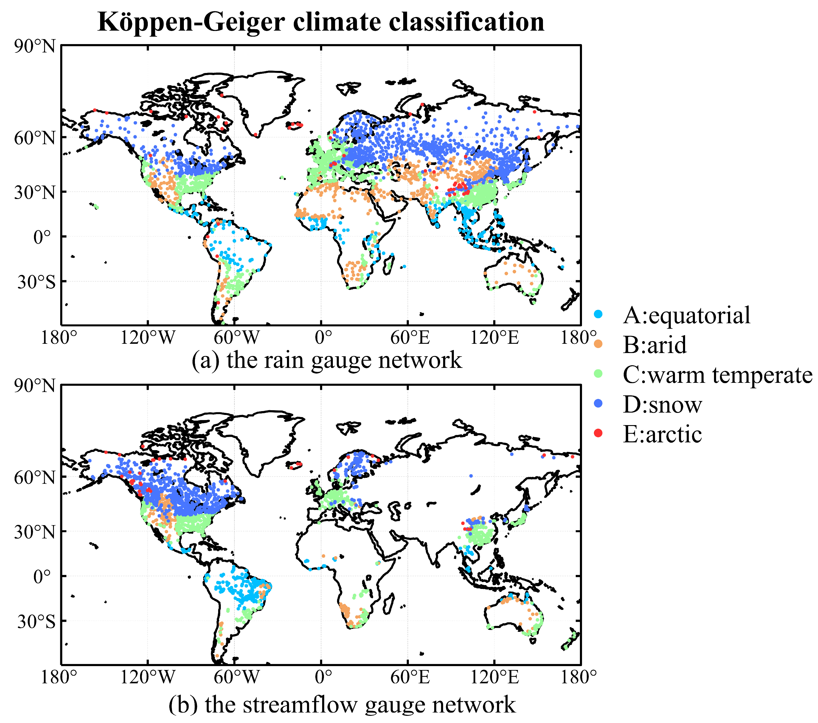
The daily rain gauge observations used in this paper were collected from the Global Summary of the Day database (https://data.noaa.gov, accessed on 1 April 2024) and the China Meteorological Administration website (http://data.cma.cn/, accessed on 1 April 2024). Two criteria were used in selecting suitable rain gauges: (1) gauges with available data from 1982 to 2015; (2) missing and invalid observations <1% of the period length. A total of 2404 gauges were selected and their distributions are shown in Figure 1a. In accordance with the Köppen–Geiger climate classification system, 2404 measurement gauges are categorized into five primary climate categories: Equatorial (A), Arid (B), Warm Temperate (C), Snow (D), and Arctic (E) [55].
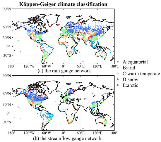
Figure 1.
Location of the basins used in this study.
2.1.3. Other Meteorological Data
The reliability of these precipitation datasets underwent evaluation through a comparative analysis with the high-resolution gridded gauge-interpolated datasets in China (CN05) [56] and Europe (E-OBS) [57]. CN05 provides daily precipitation estimates spanning the years 1961 to the present, specifically targeting the quasi-China region. This dataset encompasses a broad latitudinal range from 54° N to 18° S, with a fine spatial resolution of 0.5 degrees (https://ccrc.iap.ac.cn/resource/detail?id=228, accessed on 1 April 2024). It is produced by integrating daily precipitation measurements from 2472 Chinese national weather gauges with mainland Digital Elevation Model data using the Thin Plate Spline algorithm [58]. E-OBS is a 0.5° gridded dataset providing daily precipitation for Europe from 1950 to 2018. E-OBS is generated by interpolating data from more than 11,000 meteorological stations after undergoing accurate pre-processing (https://www.ecad.eu/download/ensembles/download.php, accessed on 1 April 2024).
The 0.25° Global Land Evaporation Amsterdam Model potential evaporation dataset from 1980 to 2015 was also employed in the simulation of runoff (https://www.gleam.eu/, accessed on 1 April 2024). It employs the Priestley and Taylor equation for the accurate estimation of potential evapotranspiration, incorporating observations of surface net radiation along with near-surface air temperature measurements [34]. Those datasets possessing spatial resolutions finer than 0.5° were resampled to a 0.5° resolution utilizing the bilinear averaging method [53,54].
2.1.4. Observed Streamflow
The daily streamflow data were systematically collected from three primary sources: the Global Runoff Data Centre (GRDC, http://www.bafg.de/GRDC/, accessed on 1 April 2024) [59], the Canadian Model Parameter Experiment database [60] and several watersheds across China. To discard erroneous observation, only gauges with an area of 2500 km2 to 50,000 km2 and for at least 10 years (not necessarily consecutive) during 1982–2015 were retained. In addition, the Hydro1K was employed to define the basin’s boundary and flow paths utilizing the ArcGIS software 10.8 [54,61]. We have compared the catchment areas delineated by hydro1k with the areas provided by GRDC, retaining only catchments with an error of less than 5%. A total of 2058 catchments were chosen, as delineated in Figure 1b, which depicts the geographical distribution of these gauges. Consistent with rain gauges, these catchments have been classified into five main climate types.
2.2. Methodology
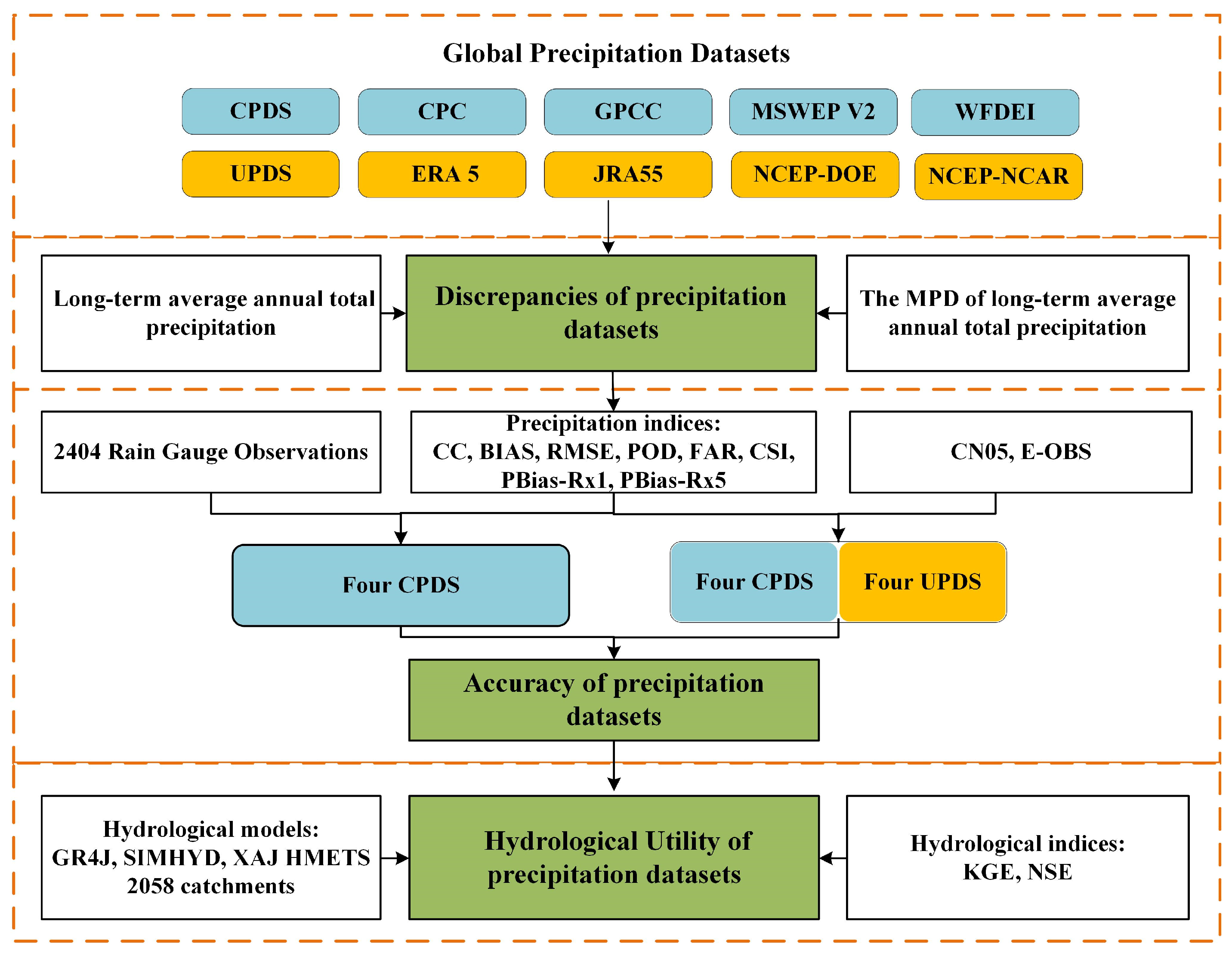
This section delineates the workflow for evaluating precipitation datasets (Figure 2), followed by details of the hydrological model and statistical analysis methods utilized in this study. All the methods considered in this study were implemented using MATLAB R2018b.
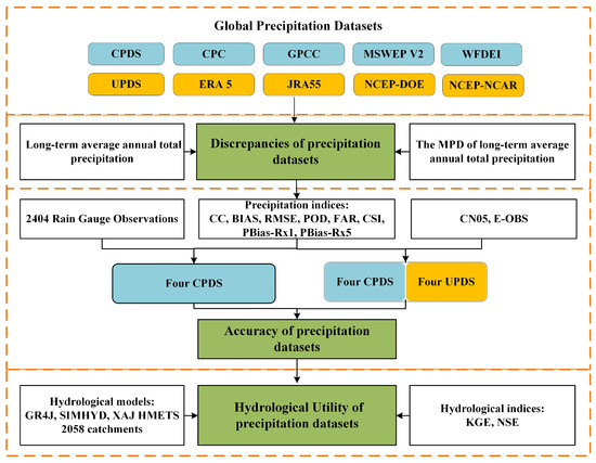
Figure 2.
The workflow for evaluating precipitation datasets used in this study.
- (1)
- The four UPDs were first evaluated on a daily timescale by comparing them with data from 2404 rain gauges worldwide.
- (2)
- The performance of the four UPDs and four CPDs (see Table 1) was then evaluated on a daily timescale using two high-resolution gridded gauge-interpolated datasets in China (i.e., CN05) and Europe (i.e., E-OBS).
- (3)
- The hydrological utility of eight precipitation datasets was subsequently assessed through hydrological modeling for 2058 catchments worldwide on a daily timescale.
2.2.1. Hydrological Models and Calibration
Numerous hydrological models have been devised and utilized for several purposes. Research conducted over the previous decade has shown that lumped and distributed hydrological models have similar accuracy for streamflow simulation. Given the scope of this study, four conceptual hydrological models with computational efficiency were implemented to assess the efficacy of eight precipitation datasets for hydrological modeling. These models have garnered widespread application in hydrological research and have demonstrated efficacy globally. The first is the GR4J [62,63]. It is a conceptual model that contains four parameters (see Table 2). It simulates the rainfall–runoff process using two storage reservoirs and a unit hydrograph-based routing scheme. In addition, the CemaNeige snow model [64,65] was added to simulate snow processes. The second is the simple lumped conceptual daily rainfall–runoff model (SIMHYD) [66,67]. SIMHYD features two linear reservoirs to calculate interflow and base flow, and a nonlinear reservoir for routing process. As with GR4J, the CemaNeige snow model was added to simulate snow processes. Therefore, it has 11 parameters in total. The third is the Xinanjiang model (XAJ) [68,69,70]. The calculation process of XAJ comprises four modules: evaporation, runoff yield, runoff sources partition, and runoff concentration. As with GR4J, the CemaNeige snow model was added to simulate snow processes. Therefore, it has 17 parameters in total. The final is the hydrological model of École de Technologie Supérieure model (HMETS) [71,72]. HMETS is a conceptual model with 21 calibration parameters. This model simulates snow accumulation, snowmelt and refreezing, evapotranspiration, infiltration, and flow routing.
The observed streamflow and simultaneous forcing data was delineated into two periods: the calibration period covering the initial 70% of the dataset, and the validation period including the subsequent 30%. The calibration process was executed employing the Shuffled Complex Evolution University of Arizona (SCE-UA) [73,74] algorithm to refine hydrological model parameters. The optimization process was driven by the objective function of Kling–Gupta Efficiency (KGE) [54,75]. In addition, all eight precipitations were employed as input to calibrate the four conceptual models against observed daily streamflow.
Table 2.
Overview of the four hydrological models.
Table 2.
Overview of the four hydrological models.
| Model | Snow Module | Simulated Processes (Number of Parameters) | References |
|---|---|---|---|
| GR4J | CemaNeige | Flow routing (1) Snow modeling (2) Vertical budget (3) | Perrin et al. [62,76] |
| SIMHYD | CemaNeige | Flow routing (1) Snow modeling (2) Vertical budget (8) | Chiew et al. [66,67] |
| XAJ | CemaNeige | Flow routing (7) Snow modeling (2) Vertical budget (8) | Zhao et al. [68,69] |
| HMETS | HMETS | Evapotranspiration (1) Flow routing (4) Snow modeling (10) Vertical budget (6) | Martel et al. [71] and Chen et al. [72] |
2.2.2. Statistical Analysis Methods
A series of statistical metrics was employed to assess the effectiveness of precipitation datasets in accurately capturing precipitation events and estimating runoff. Table 3 presents the nine metrics used for precipitation evaluation and the two metrics applied for hydrological assessment. Further elucidation of these metrics is provided in the subsequent sections.
Table 3.
List of statistical indexes used in this study.
The Maximum Percentage Difference (MPD) metric was employed to assess the discrepancies in estimating multi-annual average values among various precipitation datasets. The correlation coefficient (CC), the relative bias (BIAS) and the root mean squared error (RMSE) were adopted in this study to reflect the correlations and errors of precipitation datasets. CC quantifies the level of consistency between the two series, and the ability of each product to describe the dynamic changes of precipitation. BIAS indicates the systemic error, denoting the relative divergence in the long-term average values between two comparative series. RMSE reflects the magnitude of discrepancies between two comparative series. The Probability of Detection (POD), False Alarm Ratio (FAR) and Critical Success Index (CSI) were utilized in this study to reflect the detection capability and accuracy. POD reflects the proportion of correctly identified precipitation events. Conversely, FAR delineates the proportion of precipitation events that were erroneously forecast. CSI combines the comprehensive features of POD and FAR, which considers accurate prediction, false alarms, and missed events. In this study, any precipitation event with a value greater than 1 mm/d is considered as a precipitation event [77,78].
According to the standard set by the Expert Team on Climate Change Detection and Indices, two key variables were employed to ascertain the precision of extreme precipitation events: annual maximum 1-day precipitation amount (Rx1) and annual maximum 5-day precipitation amount (Rx5). The relative errors of gridded global precipitation and measured precipitation (PBias-Rx1 and PBias-Rx5) were calculated as evaluation metrics of extreme precipitation estimation accuracy [79]. Besides KGE, the most widely used Nash–Sutcliffe Efficiency (NSE) was also used for hydrological evaluation [80].
3. Results
3.1. Discrepancies in Annual Precipitation
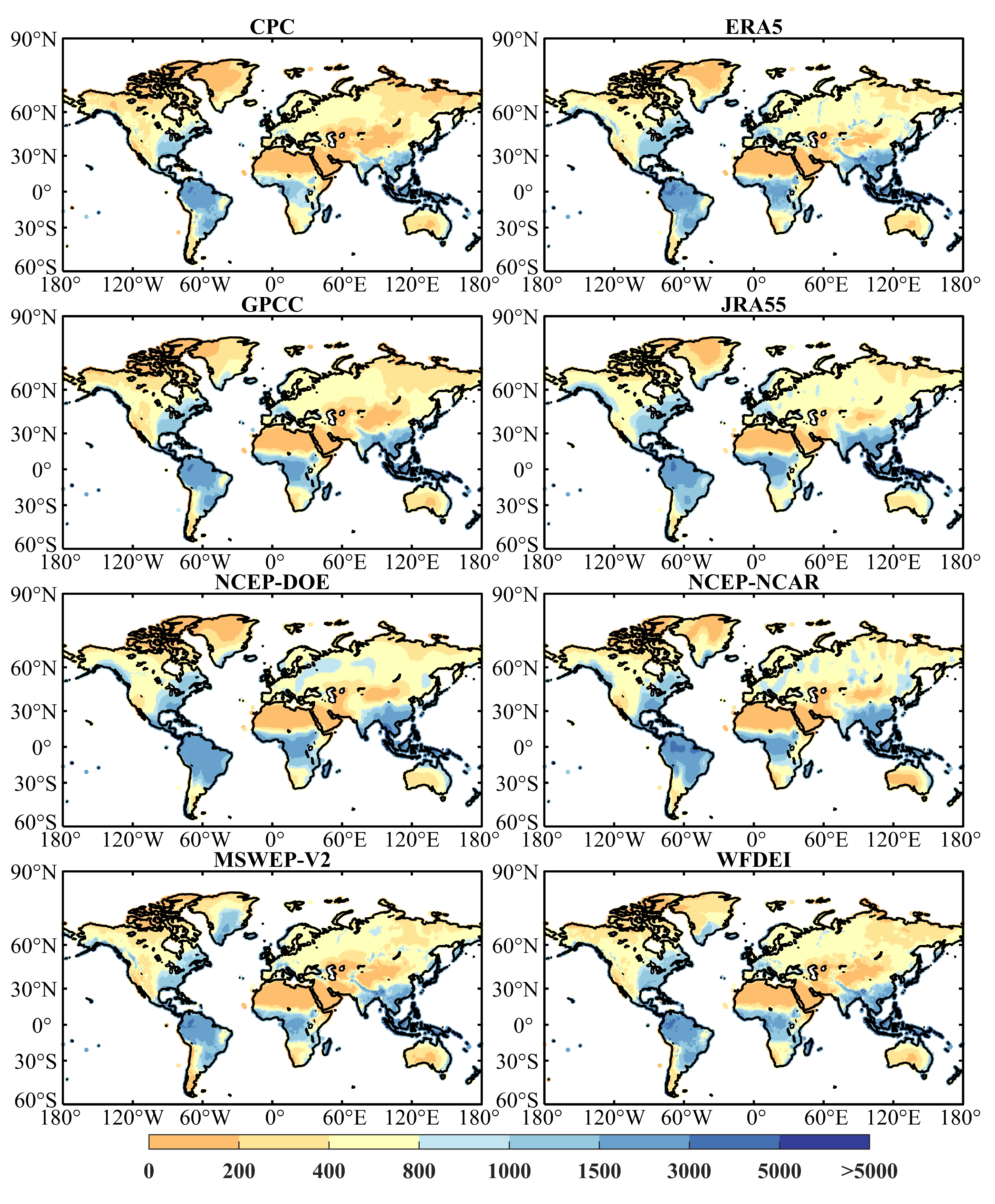
The spatial distributions of global long-term average annual precipitation of eight precipitation datasets are similar (Figure 3). The precipitation near the equator is the highest. The precipitation is significant on the east coast of the mainland due to the summer monsoons coming from the ocean. In addition, the west coast of the mainland around the Tropic of Capricorn and Cancer experiences a reduced amount of precipitation due to the subtropical high-pressure belt [81,82]. For example, West Asia and North Africa on the west coast of the mainland are dry and rainless in the prevailing northeast trade wind and the subsidence of air. However, the climatic conditions along the east coast of the mainland, exemplified by regions in East Asia, are humid and rainy due to the prevailing southerly winds from the ocean in summer. In addition, mid-latitudes and inland areas receive less precipitation as they are far from the sea, such as the northwestern region of China.
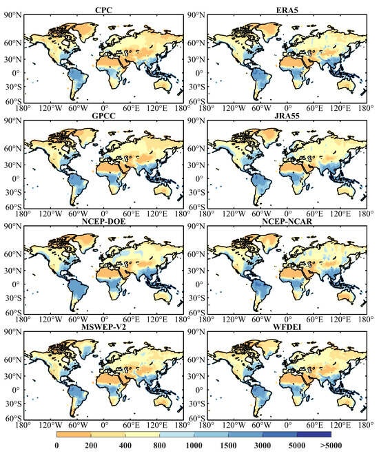
Figure 3.
Long-term average annual total precipitation (time period 1982–2015), in mm/year.
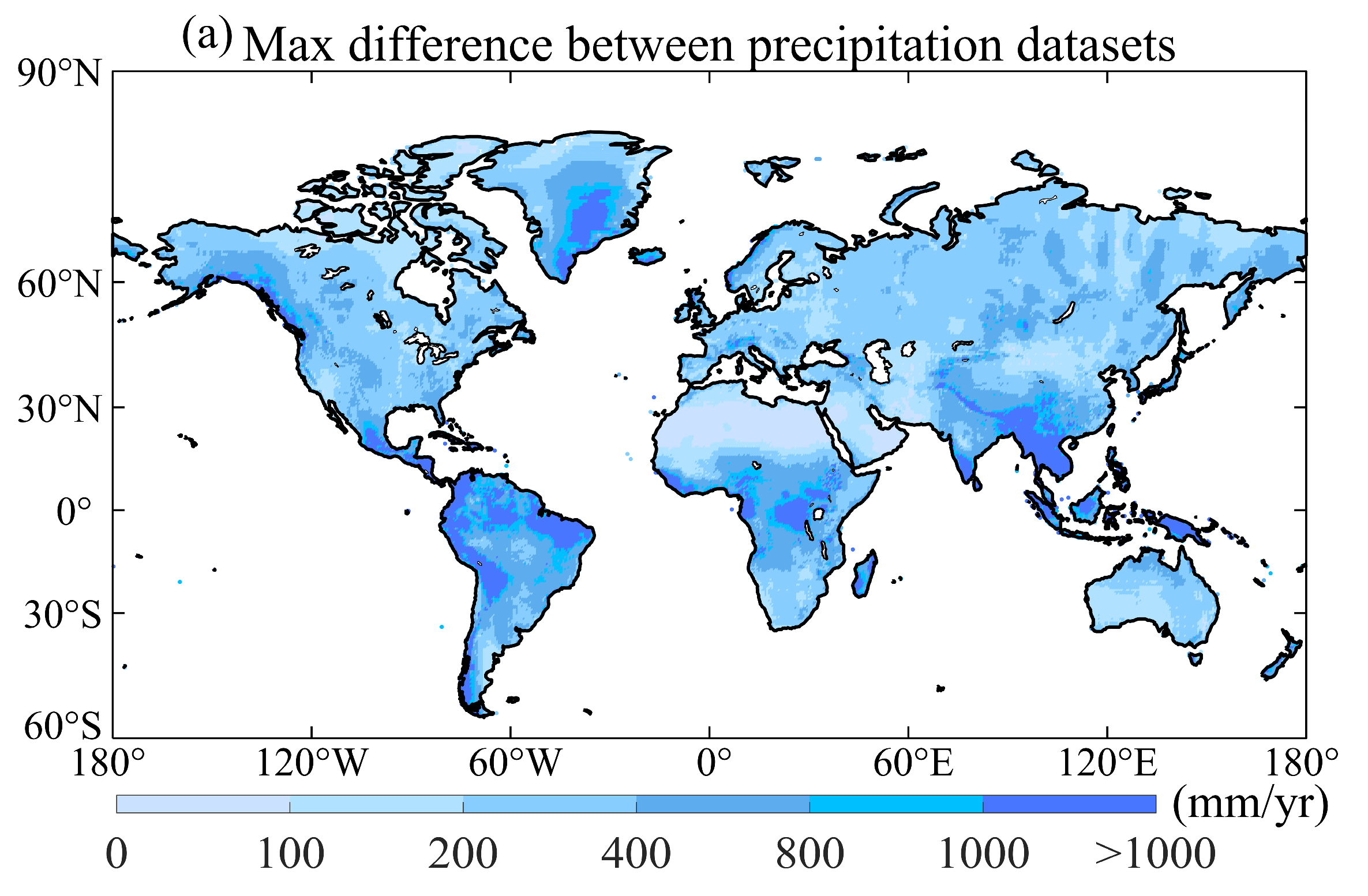
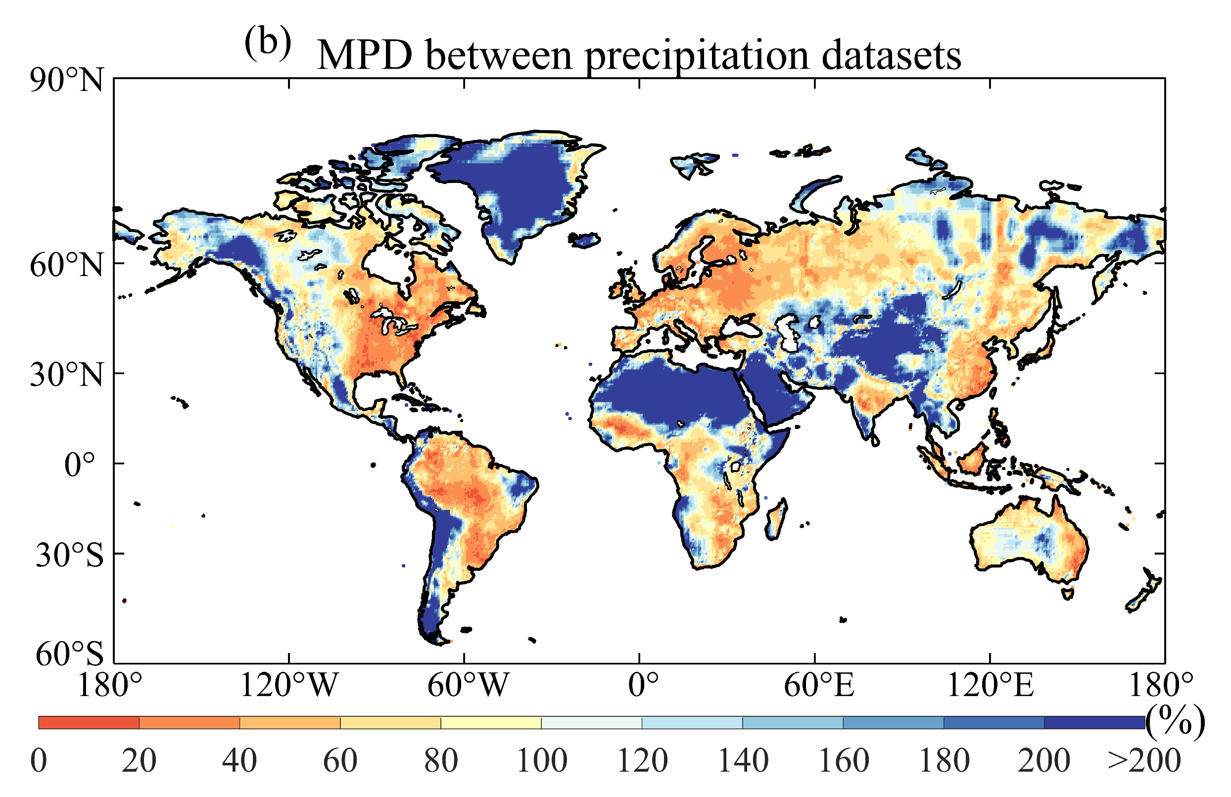
Figure 4a shows the maximum differences in long-term average annual precipitation among eight precipitation datasets, which outlines the solid spatial variability. Regions with significant differences are the Intertropical Convergence Zone (ITCZ), northwestern North America and southwestern South America. In regions like the ITCZ, minor alterations in the positioning of climatic features can result in substantial local differences in precipitation, due to large spatial gradients [83]. In addition, precipitation variations in coastal and mountainous regions exhibit more significant variability than in other areas. This phenomenon may be partly attributable to the intricate interplay between steep topographical elevations and the positioning of storm tracks [84]. Also of note is that, in general, the heavy rainfall in these areas may also result in more noticeable differences.
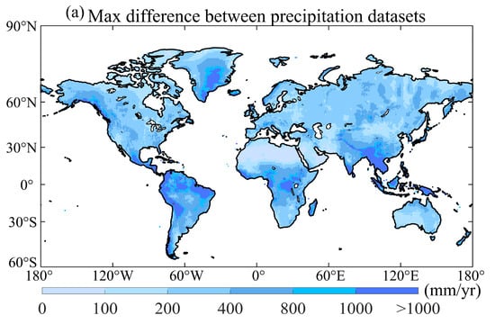
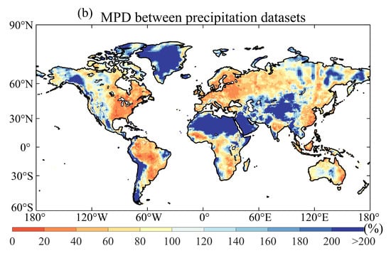
Figure 4.
(a) The spatial distribution of the maximum differences of long-term average annual precipitation between various precipitation datasets (mm/year); (b) The spatial distribution of the MPD of long-term average annual precipitation between various precipitation datasets (%).
Regarding MPD (Figure 4b), regions with more than 100% MPD are primarily situated in North Africa, Greenland, and western Asia. Most of these regions belong to arid and Arctic regions and have few rain gauges due to complex terrain and low population. Regions with less than 40% of MPD are primarily concentrated in Europe, North America and South America. Most of these regions belong to equatorial, warm temperate and snow regions and have high-density rain gauges. In total, the MPDs between precipitation datasets are marginally higher in arid and Arctic regions in comparison to other regions [12,85]. This indicates that precipitation estimates for regions with sparse measurements remain challenging and largely uncertain, and we need to be prudent in selecting the precipitation datasets for these regions.
The annual temporal evolution of global land-averaged precipitation is depicted in Figure 5. It can be seen that the interannual variability in the annual means is reasonably consistent among precipitation datasets, but with magnitudes deviating by up to 200 mm/year among the datasets. CPC estimates the lowest precipitation, which aligns with previous studies [12], followed by GPCC, WFDEI, MSWEP V2, NCEP–NCAR, NCEP–DOE, ERA5 and JRA55. In total, the annual global precipitation of the UPDs exceeds that of the CPPs, which supports the previous findings that reanalysis datasets tend to overestimate precipitation amounts [12,86]. This may be partly due to reanalysis datasets overestimating precipitation rates at higher elevations and precipitation amounts of small to medium-sized precipitation events [12,87]. The highest annual precipitation occurred in 2010 for all datasets, except for ERA5 (which occurred in 1986). The lowest precipitation occurred in 1987 for GPCC, MSWEP V2 and WFDEI, 1992 for CPC and NCEP–DOE, and 2002 for ERA5, NCEP–NCAR and JRA55. WFDEI and MSWEP V2 match well with the average of the eight precipitation datasets over the time series [88].
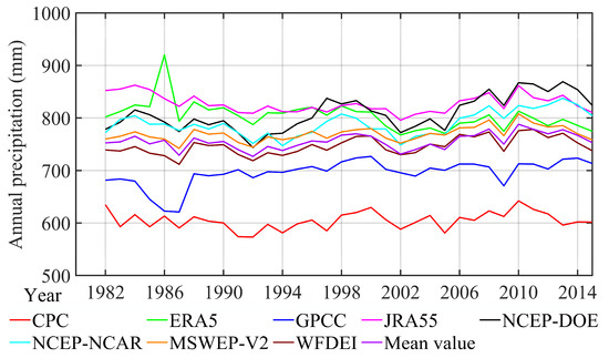
Figure 5.
Temporal evolution of global land-averaged precipitation on annual timescales (time period 1982–2015).
3.2. Evaluation of the Precipitation Datasets’ Performance Based on Ground Precipitation Observations
3.2.1. The Performance of the Four UPDs Using Gauge Observations
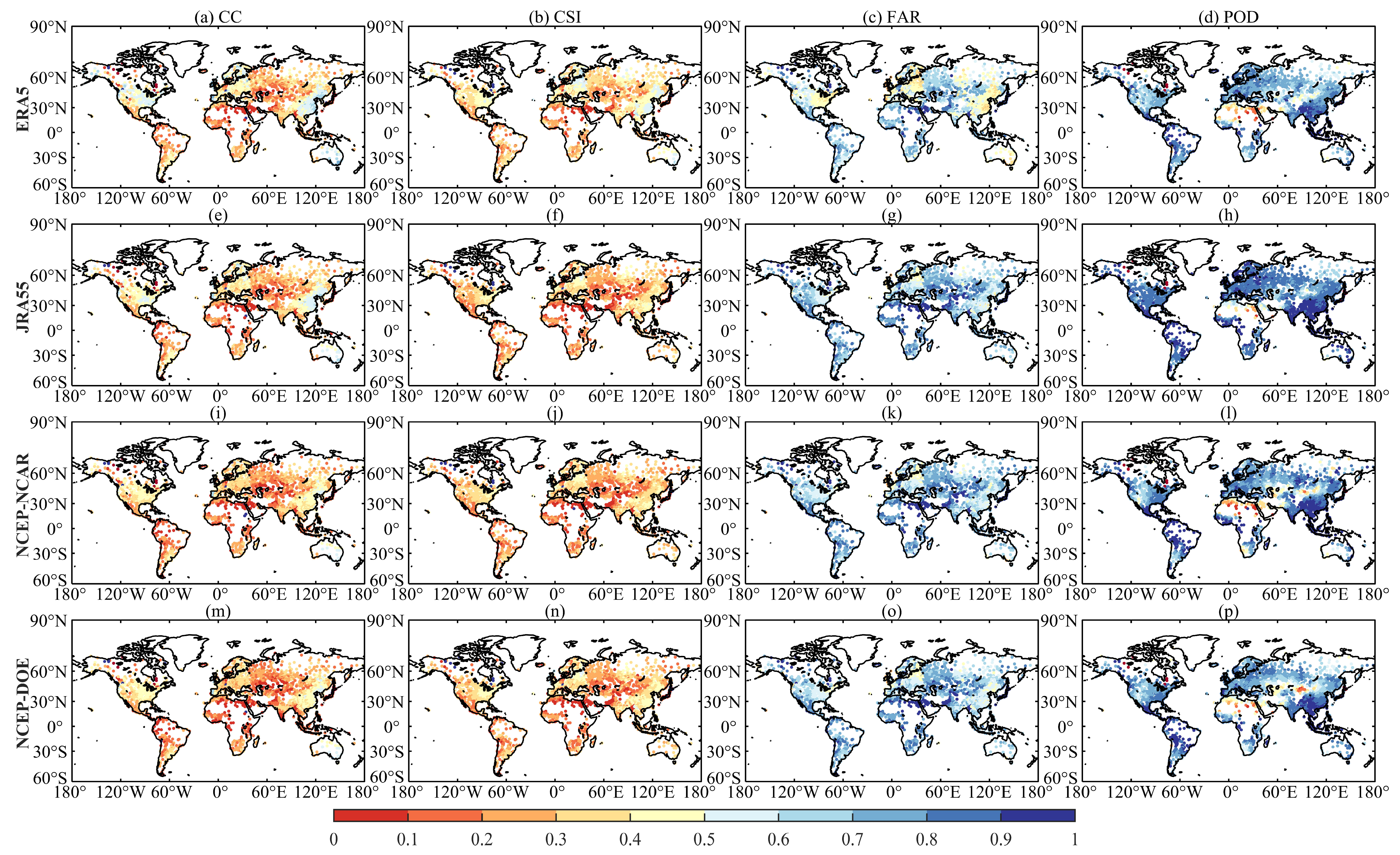
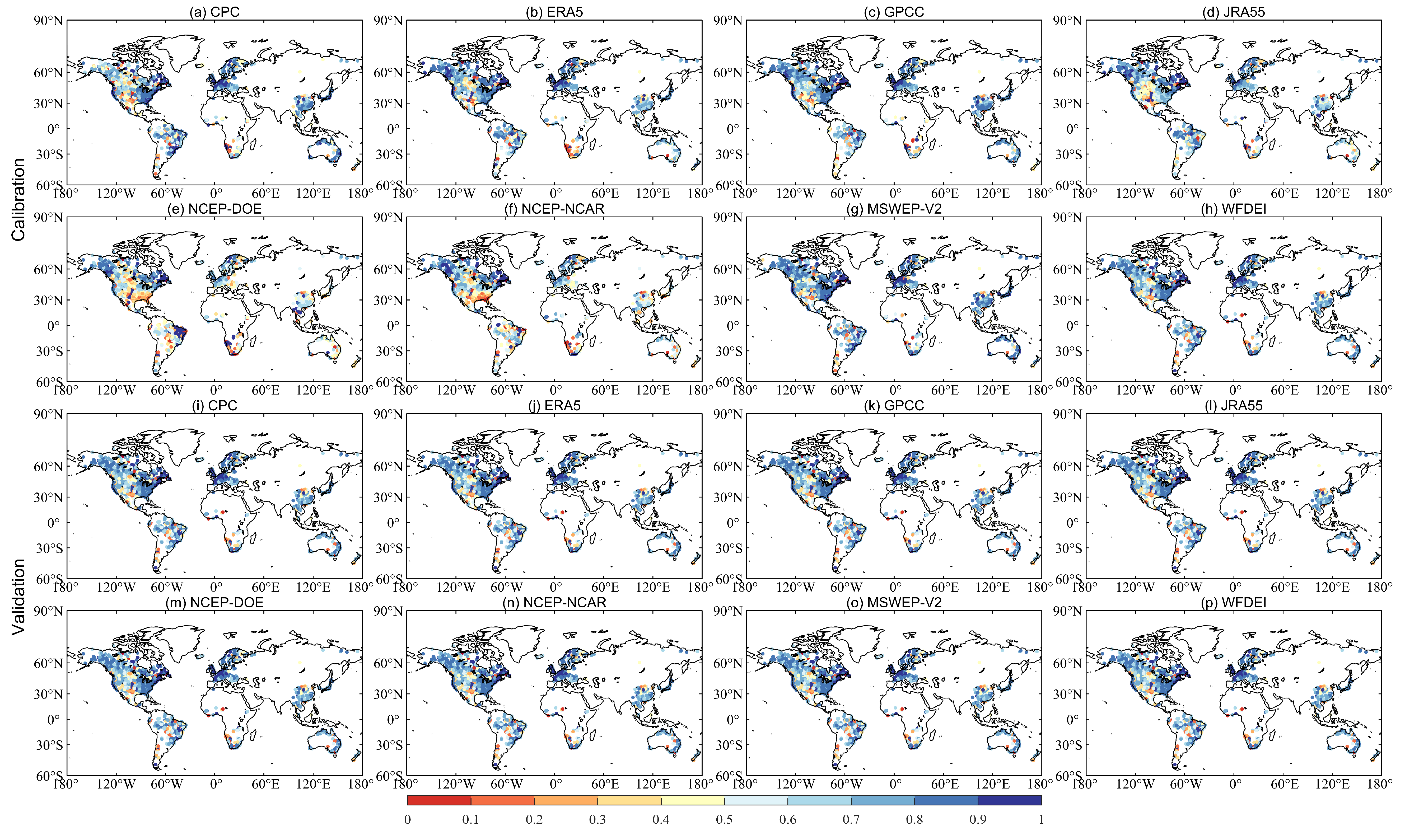
The spatial distribution of the CC, CSI, FAR and POD between the gauge observations and four uncorrected precipitation datasets are elucidated in Figure 6. Four UPDs show a similar spatial pattern for different metrics. However, different metrics exhibit pronounced spatial variability worldwide. Among them, CC, CSI and POD exhibit pronounced spatial variability. CC, CSI and POD in East Asia, Europe and northern North America are good, indicating high precipitation detection capabilities in these regions. Towards northern South America, southwest Asia and North Africa, CC, CSI and POD decreased gradually. Regarding FAR, the performance in topographically complex regions is the worst (e.g., the Hindu Kush, Rocky and Andes Mountains), demonstrating the significant challenges associated with estimating precipitation in these areas.
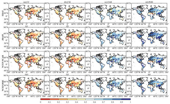
Figure 6.
The CC (the first column—(a,e,i,m)), CSI (the second column—(b,f,j,n)), FAR (the third column—(c,g,k,o)) and POD (the last column—(d,h,l,p)) between the UPDs and observed precipitation data (during 1982–2015).
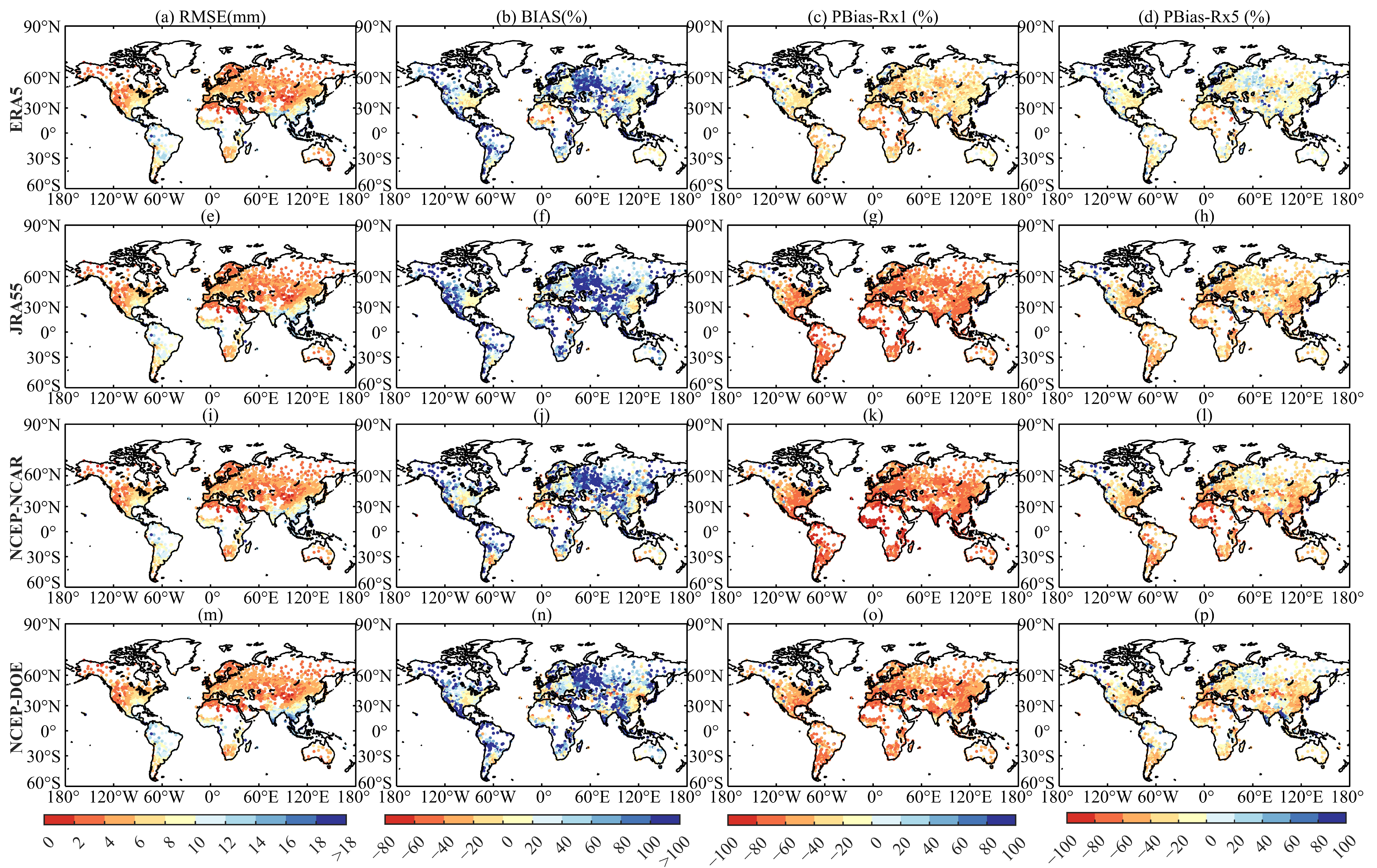
The spatial configurations of the RMSE, BIAS, PBias-Rx1 and PBias-Rx5 comparing the gauge observations with four UPDs are depicted in Figure 7. The distribution characteristics of RMSE exhibit consistency with the distribution properties of the long-term average annual total precipitation, as illustrated in Figure 3. The RMSE is highest near the equator and significant on the mainland’s east coast. Towards both sides of the tropic of Capricorn and the west coast of the mainland (e.g., northern North America, southwest Asia and North Africa), RMSE decreased gradually. Regarding BIAS, four UPDs exhibited negative biases in arid regions, and positive biases in other regions. The BIAS in warm temperate climates was consistently lower in comparison to other climatic regions. In the context of PBias-Rx1 and PBias-Rx5, it was observed that four UPDs consistently demonstrated negative biases in most regions. This indicated that these precipitations tend to underestimate the severity of extreme precipitation events. Notably, this underestimation decreases as the temporal scale increases (i.e., from 1 to 5 days).
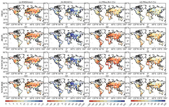
Figure 7.
The RMSE (the first column—(a,e,i,m)) and Bias (the second column—(b,f,j,n)), PBias-Rx1 (the third column—(c,g,k,o)) and PBias-Rx5 (the last column—(d,h,l,p)) between the UPDs and observed precipitation data (during 1982–2015).
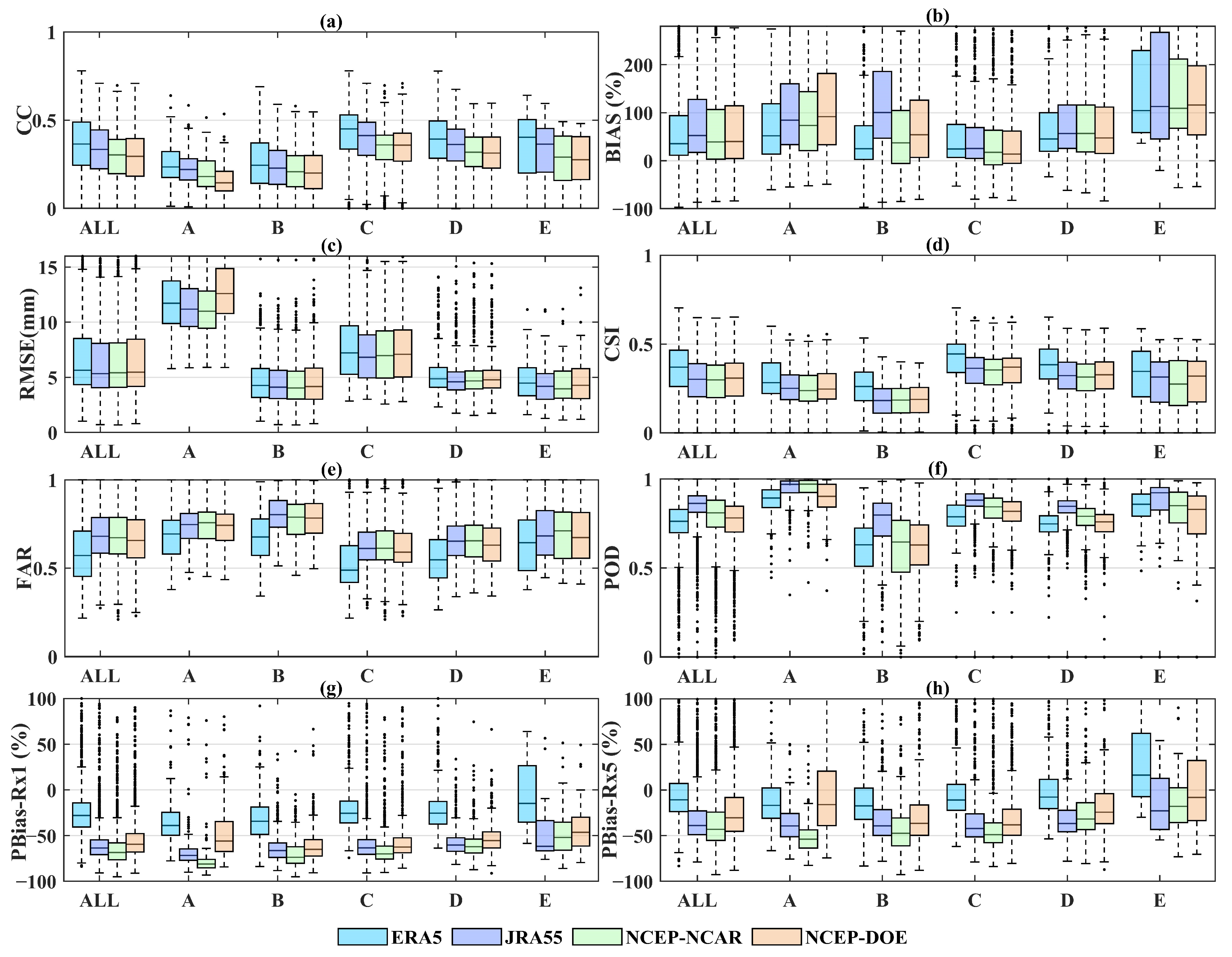
Figure 8 presents the boxplot of the eight metrics between the gauge observations and four uncorrected precipitation datasets regarding five Köppen–Geiger climate types. ERA5 outperforms other datasets in terms of CC, CSI, FAR, PBias-Rx1 and PBias-Rx5 for all climate types (with the highest median values in most regions). However, regarding BIAS, RMSE and POD, ERA5 no longer has an edge. Particularly with respect to RMSE, ERA5 underperforms against other precipitation datasets across most climate types. This indicates that ERA5 lacks the sensitivity required to identify small-sized rainfall events. ERA5 has the highest accuracy of Rx1 and Rx5 in most regions, except for the Arctic region (with median PBias-Rx1 ranging from −10.9% for the global land to −38.8% for the equatorial region). The PBias-Rx1 of the other three precipitation datasets are below −38.8%, which indicates the underestimation of extreme precipitation events. The underestimation of PBias-Rx5 is slight compared to PBias-Rx1. In particular, JRA55 performs better in warm temperate, snow, and Arctic regions regarding RMSE, while it performs well in all climate types regarding POD. However, JRA55 performs worse than other precipitation datasets for all climate types in terms of BIAS. In the evaluation of PBias-Rx1 and PBias-Rx5 metrics, JR555 is positioned third in the ranking, significantly below the performance of ERA5, yet closely approaching the second-placed NCEP–DOE. This indicates that JRA55 effectively detects rainfall events but with significant quantitative errors. NCEP–NCAR and NCEP–DOE are slightly stronger than others in terms of BIAS. NCEP–NCAR performs better in equatorial, arid and warm temperate regions, while NCEP–DOE excels in snow and Arctic regions. Nevertheless, in other dimensions, their performance is comparatively inferior.
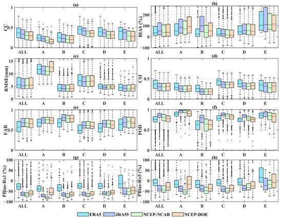
Figure 8.
Boxplots of CC (a), BIAS (b), RMSE (c), CSI (d), FAR (e), POD (f), PBias-Rx1 (g) and PBias-Rx5 (h) between gauge-observed precipitation and four UPDs in different climate region. A, B, C, D and E represent the equatorial (A), arid (B), warm temperate (C), snow (D), and Arctic (E) region, respectively.
Generally, precipitation datasets exhibit lower accuracy in arid climates compared to other climate types, as measured by most of the metrics (except for BIAS and RMSE). The short-lived and localized rainfall behavior and the sub-cloud evaporation of falling rain bring some challenges in estimating precipitation for this region. Compared to other climate regions, the BIAS of four precipitation datasets is more considerable in the Arctic region and the RMSE of four precipitation datasets is more significant in the equatorial region. The high RMSE in the equatorial region is probably due to the high precipitation intensity, extended duration rainfall, and the large amount of precipitation. The high BIAS in the Arctic region is probably due to the gauge observations not being corrected for wind-induced under-catch at high latitudes [15].
3.2.2. Performance Evaluation Using Two Gridded Gauge-Interpolated Datasets
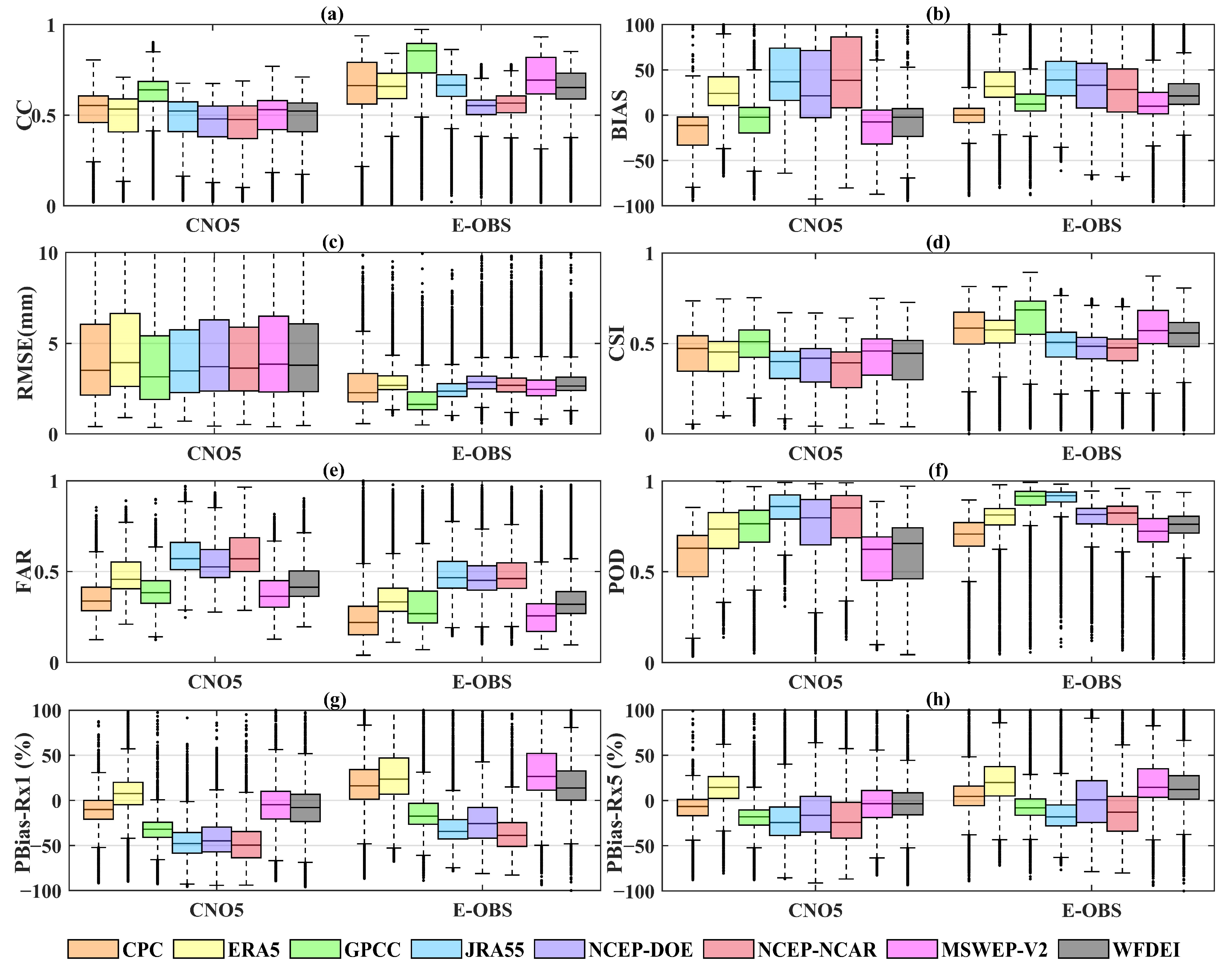
Figure 9 illustrates the daily performance of eight global precipitation datasets compared to the gridded gauge-interpolated datasets in China (CN05) and Europe (EOBS). The performance of each precipitation dataset across these two regions exhibits fundamental consistency when analyzed through various statistical measures (i.e., CC, BIAS, RMSE, CSI, FAR, POD, PBias-Rx5 and PBias-Rx1). GPCC presents a better CC, RMSE and CSI than the other seven precipitation datasets in both China and Europe, followed by CPC. CPC presents a better BIAS and FRA than the other seven precipitation datasets in both China and Europe, followed by GPCC and MSWEP V2. These indicate smaller systematic errors of gauged-based precipitation datasets in these two regions. The high BIAS and RMSE of the UPDs may be partly due to the significant overestimation of precipitation amounts, as shown in Figure 5. However, in terms of POD, JRA55 presents a better POD than the other seven precipitation datasets in both China and Europe. CPC has the most miniature POD. The ranking of the accuracy for extreme precipitation metrics (median PBias-Rx1) is MSWEP V2 (−4.8%), ERA5 (7.6%), WFDEI (−7.9%), CPC (−10.2%), GPCC (−32.1%), NCEP–DOE (−44.8%), JRA55 (−47.8%) and NCEP–NCAR (−49.6%) in China (CN05), and WFDEI (13.7%), CPC (16.1%), GPCC (−17.4%), ERA5 (23.6%), NCEP–DOE (−25.6%), MSWEP V2 (26.5%), JRA55 (−34.4%), and NCEP–NCAR (−38.7%) in Europe (E-OBS). Most precipitation datasets tend to underestimate Rx1day and Rx5day in China, except for ERA5. In Europe, ERA5, CPC, MSWEP V2 and WFDEI tend to overestimate Rx1day, Rx5day and GPCC, JRA55, NCEP-NSAR and NCEP–DOE tend to underestimate Rx1day, Rx5day. It could be concluded that CPC, WFDEI and GPCC show great accuracy as an extreme precipitation index. Overall, the corrected precipitation datasets (CPDs, GPCC, CPC, MSWEP V2 and WFDEI) perform slightly better than the UPDs (ERA5, JRA55, NCEP-NSAR and NCEP–DOE).
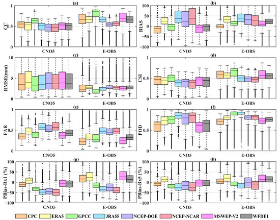
Figure 9.
Boxplots of CC (a), BIAS (b), RMSE (c), CSI (d), FAR (e), POD (f), PBias-Rx1 (g) and PBias-Rx5 (h) between two high-resolution gridded gauge-interpolated datasets (CN05 and EOBS) and eight precipitation datasets.
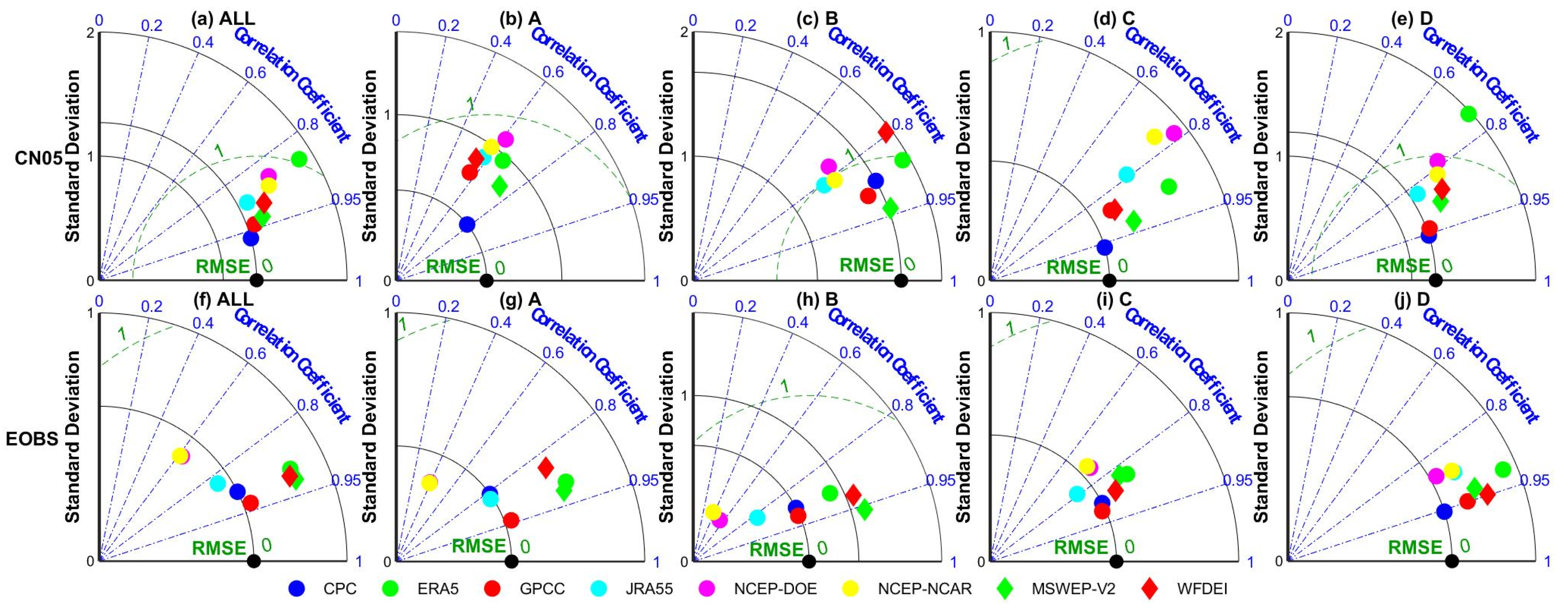
The Taylor diagram of different precipitation datasets in 0.5° grids of China and Europe using CN05 and EOBS as references has been plotted (Figure 10). In general, CPC is closer to the gridded gauge-interpolated datasets in China for most climate types (except for the arid region), followed by GPCC. In Europe, GPCC is closer to the gridded gauge-interpolated datasets for most climate types (except for the snow region). Generally, precipitation datasets perform relatively better in warm temperate and equatorial regions than in arid and snow regions. Compared to arid and snow regions, precipitation datasets in other regions have a smaller deviation from the gridded gauge-interpolated dataset. The difference in standard deviation between different precipitation datasets is more significant in the arid region, especially in China.
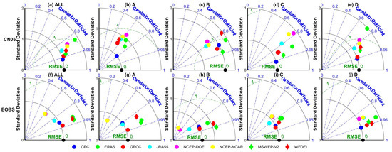
Figure 10.
Taylor diagram for comparison of different precipitation datasets in China (CN05) and Europe (EOBS) in terms of five Köppen–Geiger climate types (1982–2015). A, B, C, D and E represent the equatorial (A), arid (B), warm temperate (C), snow (D), and Arctic (E) region, respectively.
3.3. Evaluation of Precipitation Datasets’ Performance Based on Hydrological Modeling
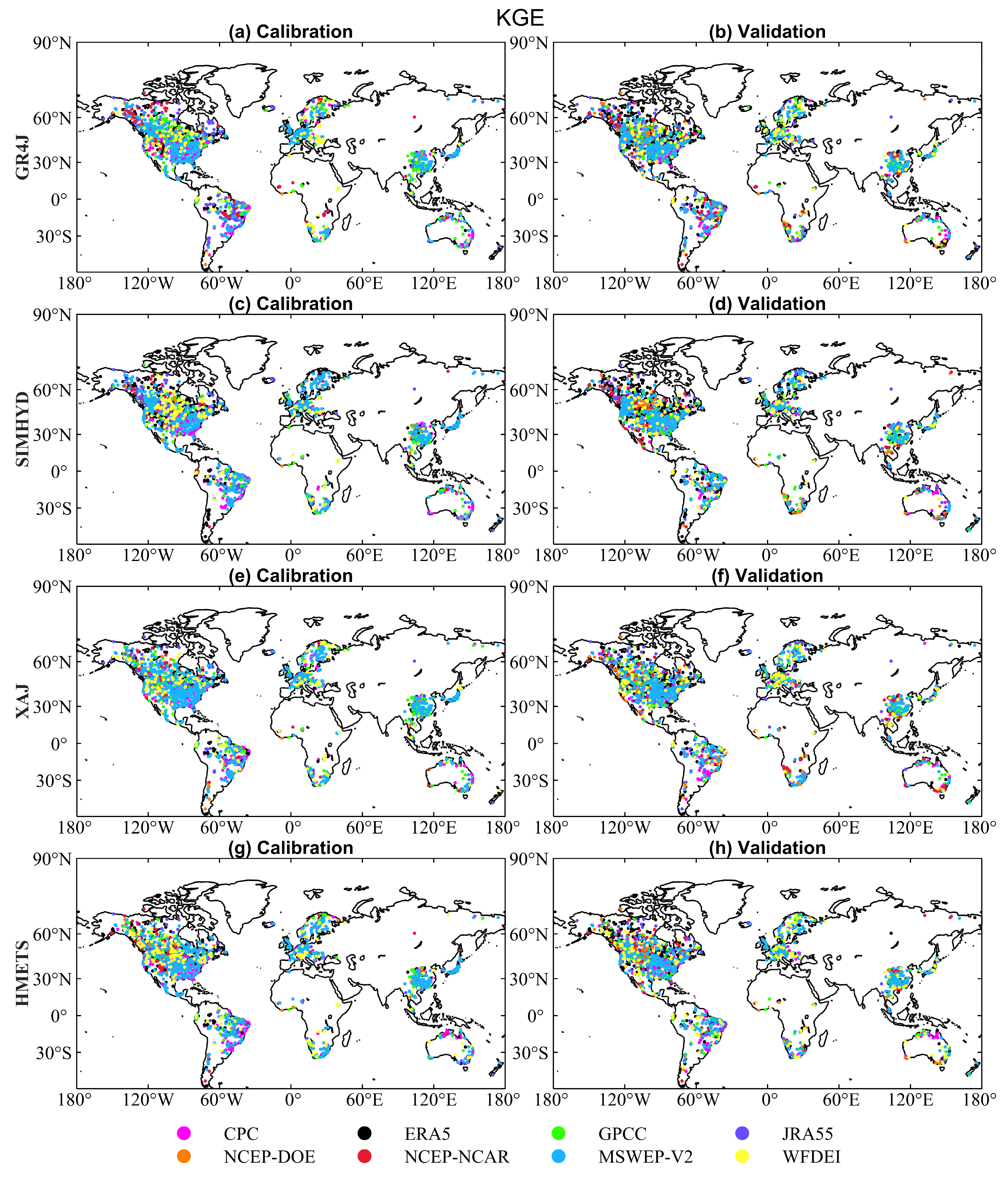
The hydrological utilities of eight precipitation datasets have been assessed using four hydrological models across 2058 global catchments. Figure 11 shows the global maps with KGE values obtained from GR4J (see the Figure A1, Figure A2 and Figure A3 for Spatial patterns of SIMHYD, XAJ and HMETS) driven by eight precipitation datasets in both calibration (Figure 11a–h) and validation periods (Figure 11i–p). The precipitation datasets exhibit similar behavior across continental areas. That is, the KGE values for most catchments in southern China, eastern Canada, the United States, and along the Atlantic Coast of Europe exceed 0.8. The excellent model performances of those regions are likely to be due to the dense network of precipitation gauges and the high quality of precipitation data. However, catchments in areas such as the Andes (South America), northwest China, and the American tropics exhibit low KGE values due to the intricate topography and the absence of precipitation gauges.
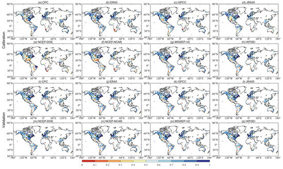
Figure 11.
Spatial distribution of KGE values obtained from GR4J driven by eight precipitation datasets in calibration (a–h) and validation periods (i–p).
Figure 12 presents the best performing precipitation datasets (i.e., with the highest calibration and validation KGE) for each catchment (see Figure A4 for Spatial patterns of NSE). The ranking of the best performed precipitation dataset in GR4J (i.e., the proportion of catchments the dataset exhibited optimal performance) is MSWEP V2 (33.1%), CPC (16.3%), GPCC (15.4%), JRA55 (12.1%), ERA5 (9.3%), WFDEI (7.8%), NCEP–NCAR (5.2%) and NCEP–DOE (0.8%) in the calibration period, and MSWEP V2 (27.2%), CPC (13.1%), GPCC (12.1%), JRA55 (9.4%), ERA5 (22.6%), WFDEI (6.9%), NCEP–NCAR (5.2%) and NCEP–DOE (3.5%) in the validation period. Comparable outcomes are achieved in other models. The MSWEP V2, in combination with various satellites, gauges, and reanalysis products, outperforms other precipitation datasets.
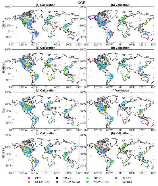
Figure 12.
Spatial distribution of best performing precipitation datasets. For each catchment, color indicates which precipitation dataset produced the best KGE.
To further explore the impact of climatic conditions on the efficacy of precipitation datasets in runoff simulation affected by climatic conditions and whether the best performing precipitation datasets vary depending on the climate type, Table 4 shows the median KGE values of four hydrological models driven by eight precipitation datasets for different climate types. The graphic demonstration of the comparison results is shown in Figure 13 (see Figure A5 for NSE)). The analysis reveals that, in comparison to the other four climatic classifications, the performance of these models is markedly inferior within arid climate regions (with median KGE ranging from 0.39 to 0.65), as evidenced across all precipitation datasets. The intricate hydrological behavior, characterized by extreme floods and droughts, along with the variability in meteorological and hydrological conditions, presents significant challenges to hydrological modeling in these regions [89,90,91]. The hydrological performance in warm temperate regions is best (with the median KGE values fluctuating between 0.47 and 0.84), which may be partly because of the presence of dense monitoring networks. In addition, MSWEP V2 demonstrates superior performance in comparison to others across most climate regions, with the exception of the Arctic region. In the Arctic region, the efficacy of MSWEP V2 exhibits no significant deviation from those obtained from optimal precipitation (with the median KGE values no more than 0.03). Overall, the MSWEP V2 model maintains a relatively stable performance across diverse climatic conditions. The four UPDs, especially the NCEP–DOE and NCEP–NCAR datasets, perform much worse than the other four CPDs in the equatorial, warm temperate and arid regions. However, in the snow and Arctic regions, the performance order changed. The gauged-based CPC demonstrates the poorest performance, as evidenced by the lowest KGE value. The NCEP–DOE and NCEP–NCAR show a substantial rise in these two regions, which is in line with previous evaluations [92].
Table 4.
Median calibration KGE scores for the four hydrological models driven by eight precipitation datasets. Values in bold represent the highest score in each group.
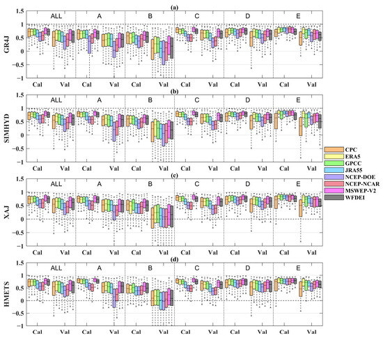
Figure 13.
Boxplots of KGE values of different precipitation datasets for both calibration period (Cal) and validation period (Val) in different climate regions ((a) GR4J, (b) SIMHYD, (c) XAJ, (d) HMETS). A, B, C, D and E represent the equatorial (A), arid (B), warm temperate (C), snow (D), and Arctic (E) region, respectively.
4. Discussion
Based on the findings of the present investigation, it is clear that there is no one precipitation dataset that excels in every aspect. This emphasizes the uncertainties and errors within existing precipitation datasets and the necessity for meticulous evaluation to ascertain their suitability for particular utilities and climate conditions. The uncertainties are usually induced by errors from data sources, estimation procedures, quality control schemes, and scaling effects. For satellite-based precipitation, the errors may stem from the retrieval algorithms, the sensor used and the sampling frequency. The observational constraints, assimilation techniques and parameterization strategies may lead to uncertainties in reanalysis datasets. Uncertainties in gauge-based precipitation can be due to the network density, the interpolation method and the inconsistent time series of gauges [8,12,50]. As found in the current study, precipitation datasets show poor performance in regions with sparse measurements.
The scaling effects also lead to uncertainty of precipitation, e.g., the spatial and temporal resolution. Behrangi et al. [93] quantified the errors attributed to temporal and spatial sampling of precipitation events and concluded that the error of precipitation datasets decreases with increasing spatial and time resolution. Peng et al. [78] found that, while precipitation products demonstrate a robust correlation with rain gauge measurements at the annual and seasonal scales, their accuracy decreases when evaluated on a monthly scale. In addition, the spatial discontinuities between the catchment scale and grid scale may lead to uncertainties when using gridded precipitation as input for runoff simulation. For example, the MSWEP V2 precipitation dataset, which excels in runoff simulation, does not demonstrate clear advantages in precipitation estimation accuracy, especially for extreme precipitation. High spatial and temporal resolution precipitation can offer more detailed precipitation patterns, thereby improving the reliability of precipitation estimations and reducing the uncertainties in hydrological utility [78]. The validation conducted here shows the imperative need for advancements in precipitation datasets. Enhanced spatial and temporal resolution combined with expanded temporal coverage is crucial for achieving these improvements.
The fidelity of various precipitation datasets in capturing extreme precipitation events exhibits regional variability. In this study, four uncorrected precipitations underestimate Rx1 and Rx5 in most climate regions. The results of Rx5 showed overall improvement compared to Rx1. The bias of Rx5 in most regions is within 50%. The degree of bias has improved, and the range of severe overestimates or underestimates has narrowed. Similar results were obtained when compared to CN05. However, ERA5, CPC, MSWEP V2, and WFDEI overestimated extreme precipitation with positive PBias-Rx1 and PBias-Rx5 compared with E-OBS. Our results provided obvious evidence that precipitation datasets show poor accuracy in extreme precipitation events, even though estimation accuracy improves as the time scale increases (i.e., from 1 to 5 days). The poor accuracy of the maximum 1-day precipitation amount makes it difficult to meet the needs of risk management. Extreme precipitation events can result in devastating consequences, such as storms, floods, mudslides, and other related disasters, presenting a significant risk to human life and property. Climate change significantly impacts the increase in extreme precipitation events. In the future, a significant proportion of meteorological stations may encounter more intense extreme precipitation events than have been recorded historically [79]. The non-stationarity of precipitation may result in previously gauged stations becoming data-sparse regions, increasing our dependence on precipitation products [94]. This serves as a reminder that it is essential to improve the ability to faithfully represent extreme events, rather than simply increasing the quantity of precipitation products.
5. Conclusions
This research undertook a thorough evaluation of eight global grid precipitation datasets (i.e., CPC, GPCC, ERA5, NCEP–NCAR, NCEP–DOE, MSWEP V2, JRA55 and WFDEI) from multiple aspects. The daily observations from 2404 gauges and two high-resolution gridded gauge-interpolated datasets (i.e., CNO5 and E-OBS) were employed to assess the precipitation datasets at the site and regional scales. Subsequently, four conceptual hydrological models were employed to evaluate the efficacy of different precipitation datasets on hydrological modeling over 2058 catchments from five climate regions. The following conclusions can be made:
All precipitation datasets are capable of capturing the interannual variability observed in the mean annual precipitation values. The deviations in estimated annual precipitation were up to 200 mm/year among these precipitation datasets. The degree of variability in precipitation estimates also differed across regions. Regions with significant differences are the Intertropical convergence zone, northwestern North America and southwestern South America. Regions with more than 100% MPD are mainly distributed in North Africa, Greenland and western Asia, primarily arid and Arctic regions with sparse measurements compared to other regions.
The accuracy difference of these four uncorrected precipitation datasets at the gauge site scale varies according to statistical metrics across different climate regions. Generally, ERA5 surpasses others for all climate regions with the highest median CC, CSI and FAR and least bias of Rx1 and Rx5. Regionally, the gauged-based dataset GPCC is more correlated with CN05 and E-OBS, closely followed by CPC and blended dataset MSWEP V2. Overall, the CPDs perform slightly better than the UPDs. The high BIAS and RMSE of the UPDs may be partly due to the significant overestimation of precipitation amounts. Notable disparities are observed across various climatic regions, with precipitation datasets exhibiting significantly inferior performance in arid regions than in the other four climate types for most metrics.
The differences among different datasets in hydrological simulations are significant. The datasets that incorporate daily gauge observations (MSWEP V2, CPC, GPCC and WFDEI) outperform others. The efficacy of hydrological modeling with different precipitation datasets is climate dependent, with lower median KGE values (ranging from 0.39 to 0.65) in arid regions compared to the other four climate types. The four UPDs perform much worse in the equatorial, arid and warm temperate regions. However, these UPDs demonstrate a marked improvement in performance in the snow and Arctic regions. Among the eight precipitation datasets, MSWEP V2 posted a stable performance with the highest KGE and NSE values in most climate regions.
Overall, the thorough evaluation investigates the accuracy and hydrological utility of different precipitation datasets under different climate conditions and highlights the strengths and limitations of individual datasets. This information holds significance in providing a valuable reference for readers where care is required when undertaking analyses. The study still has some limitations. For example, only precipitation datasets covering the global land surface and with a time span greater than 30 years are considered in this study. The latest precipitations with short temporal coverage are not included in the evaluation. Furthermore, only lumped hydrological models were used in this study, and distributed hydrological models were not considered. Therefore, further studies with various latest high-resolution precipitation datasets and distributed hydrological models should be conducted to generalize the conclusions of this study.
Author Contributions
Conceptualization, W.Q.; Data curation, W.Q. and J.C.; Formal analysis, W.Q., S.W. and J.C.; Funding acquisition, W.Q.; Investigation, W.Q., S.W. and J.C.; Methodology, W.Q. and S.W.; Supervision, W.Q.; Validation, W.Q. and J.C.; Visualization, W.Q. and J.C.; Writing—original draft, W.Q., S.W. and J.C.; Writing—review and editing, W.Q., S.W. and J.C. All authors have read and agreed to the published version of the manuscript.
Funding
This research was funded by the Science and Technology Program of Gansu Province, grant number 22JR11RA143 and the Young Scholars Science Foundation of Lanzhou Jiaotong University, grant number 1200061160.
Data Availability Statement
The datasets used in this study are available by writing to the authors.
Acknowledgments
The authors would like to acknowledge all of the organizations for providing the precipitation datasets and other data. The authors also thank the editors and reviewers for their valuable comments and thoughtful suggestions.
Conflicts of Interest
The authors declare no conflicts of interest.
Abbreviations
| Precipitation | |
| CPC | Climate Precipitation Center dataset |
| GPCC | Global Precipitation Climatology Center dataset |
| ERA5 | European Centre for Medium-Range Weather Forecast Reanalysis 5 |
| NCEP–NCAR | National Centers for Environmental Prediction–National Center for Atmosphere Research |
| NCEP–DOE | National Centers for Environmental Prediction–Department of Energy |
| JRA55 | Japanese 55-year ReAnalysis |
| WFDEI | WATCH forcing data methodology is applied to ERA-Interim dataset |
| MSWEP V2 | Multi-source weighted-ensemble precipitation V2 |
| UPDs | Uncorrected precipitation datasets |
| CPDs | Corrected precipitation datasets |
| Köppen–Geiger climate classification | |
| A | Equatorial |
| B | Arid |
| C | Warm temperate |
| D | Snow |
| E | Arctic |
| Other Data | |
| CN05 | A high-quality gridded daily observation dataset over China |
| E-OBS | European high-resolution gridded dataset |
| GRDC | Global Runoff Data Centre |
| Hydrological model | |
| GR4J | Génie Rural à 4 Paramètres Journalier model |
| SIMHYD | Simple lumped conceptual daily rainfall-runoff model |
| XAJ | Xinanjiang model |
| HMETS | Hydrological model of École de Technologie supérieure model |
| Criteria | |
| KGE | Kling–Gupta efficiency |
| NSE | Nash–Sutcliffe Efficiency |
| MPD | Maximum Percentage Difference |
| CC | Correlation coefficient |
| BIAS | Relative bias |
| RMSE | Root mean squared error |
| POD | Probability of Detection |
| FAR | False Alarm Ratio |
| CSI | Critical Success Index |
| Rx1 | annual maximum 1-day precipitation amount |
| Rx5 | annual maximum 5-day precipitation amount |
| Others | |
| ITCZ | Intertropical Convergence Zone |
Appendix A
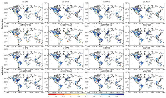
Figure A1.
Spatial distribution of KGE values obtained from SIMHYD driven by eight precipitation datasets in calibration (a–h) and validation periods (i–p).
Figure A1.
Spatial distribution of KGE values obtained from SIMHYD driven by eight precipitation datasets in calibration (a–h) and validation periods (i–p).
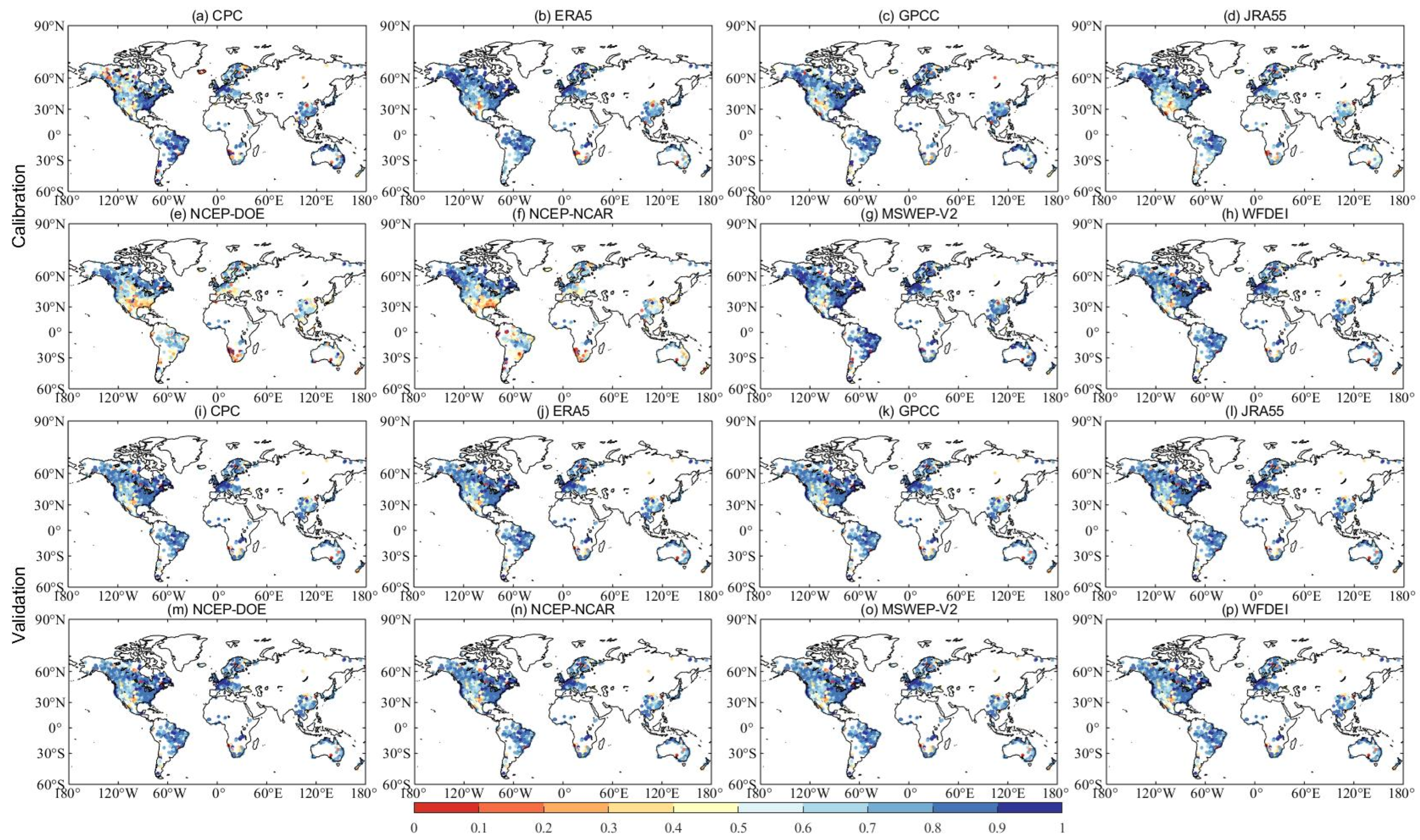
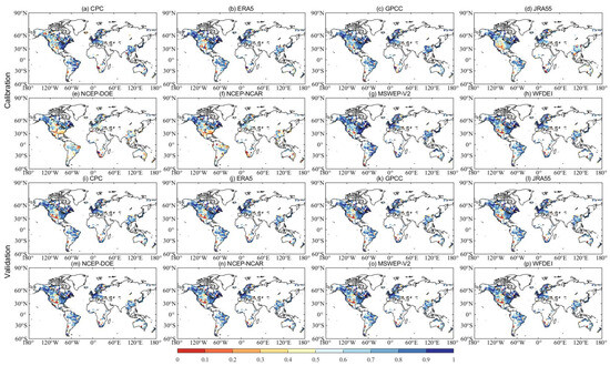
Figure A2.
Spatial distribution of KGE values obtained from XAJ driven by eight precipitation datasets in calibration (a–h) and validation periods (i–p).
Figure A2.
Spatial distribution of KGE values obtained from XAJ driven by eight precipitation datasets in calibration (a–h) and validation periods (i–p).
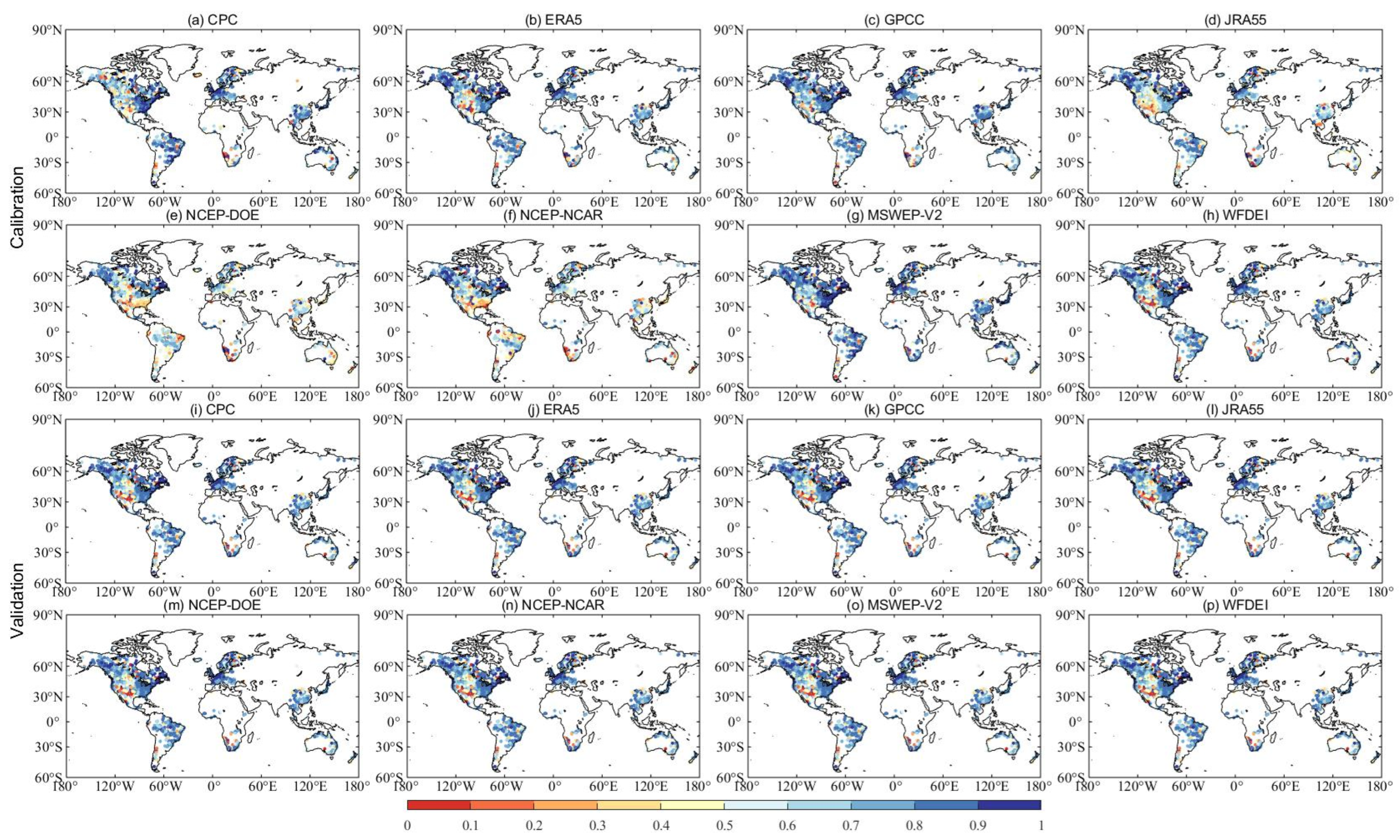
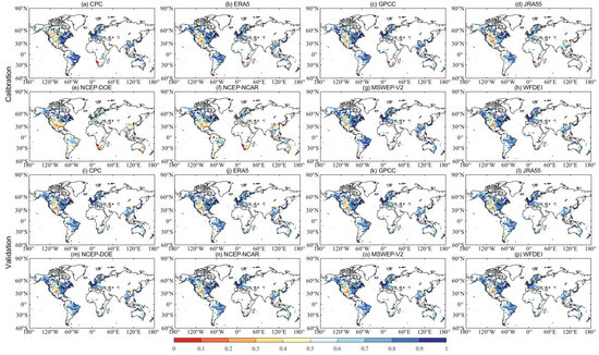
Figure A3.
Spatial distribution of KGE values obtained from HMETS driven by eight precipitation datasets in calibration (a–h) and validation periods (i–p).
Figure A3.
Spatial distribution of KGE values obtained from HMETS driven by eight precipitation datasets in calibration (a–h) and validation periods (i–p).
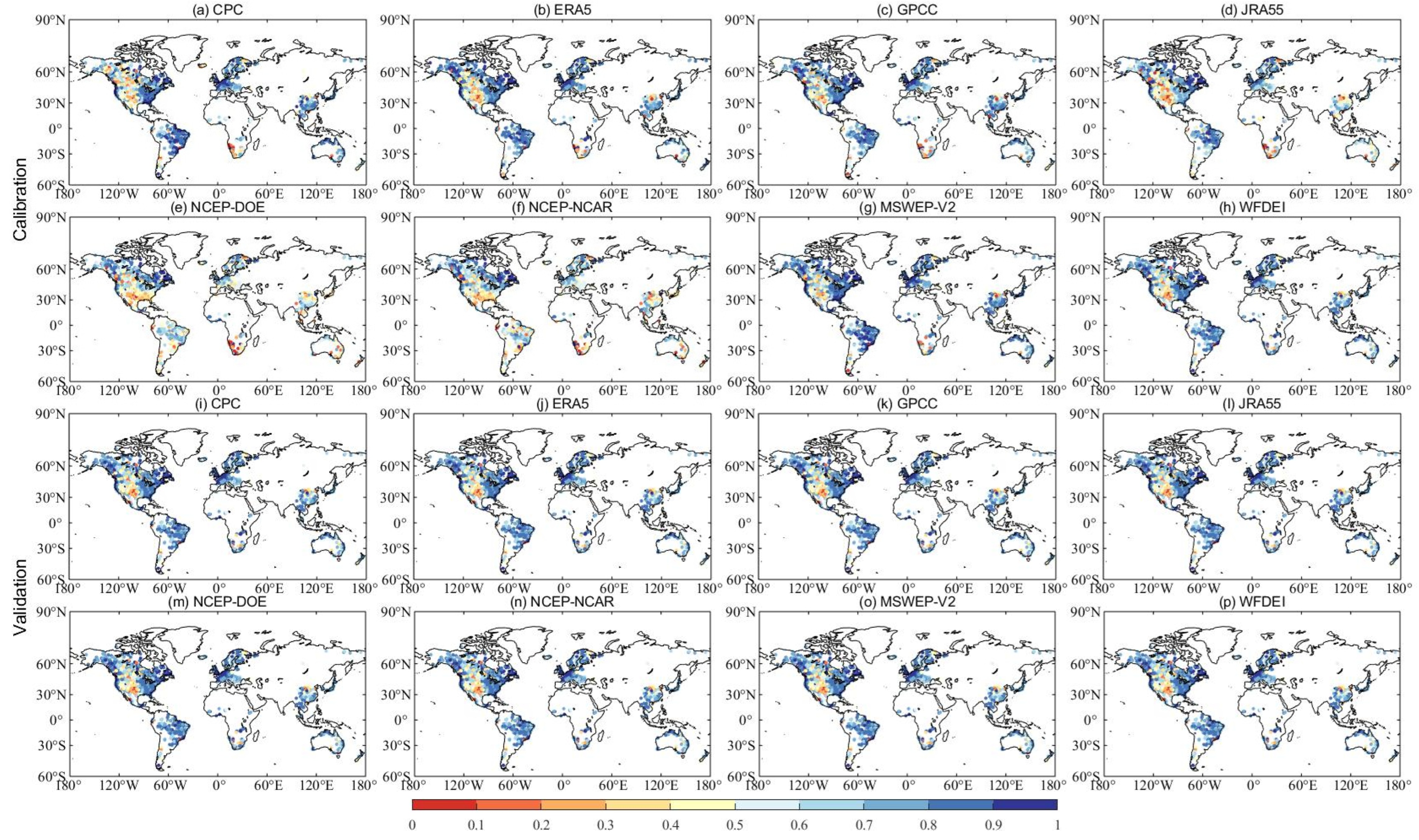
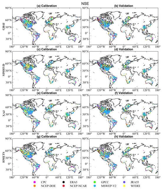
Figure A4.
Spatial distribution of best performing precipitation datasets. For each catchment, color indicates which precipitation dataset produced the best NSE.
Figure A4.
Spatial distribution of best performing precipitation datasets. For each catchment, color indicates which precipitation dataset produced the best NSE.
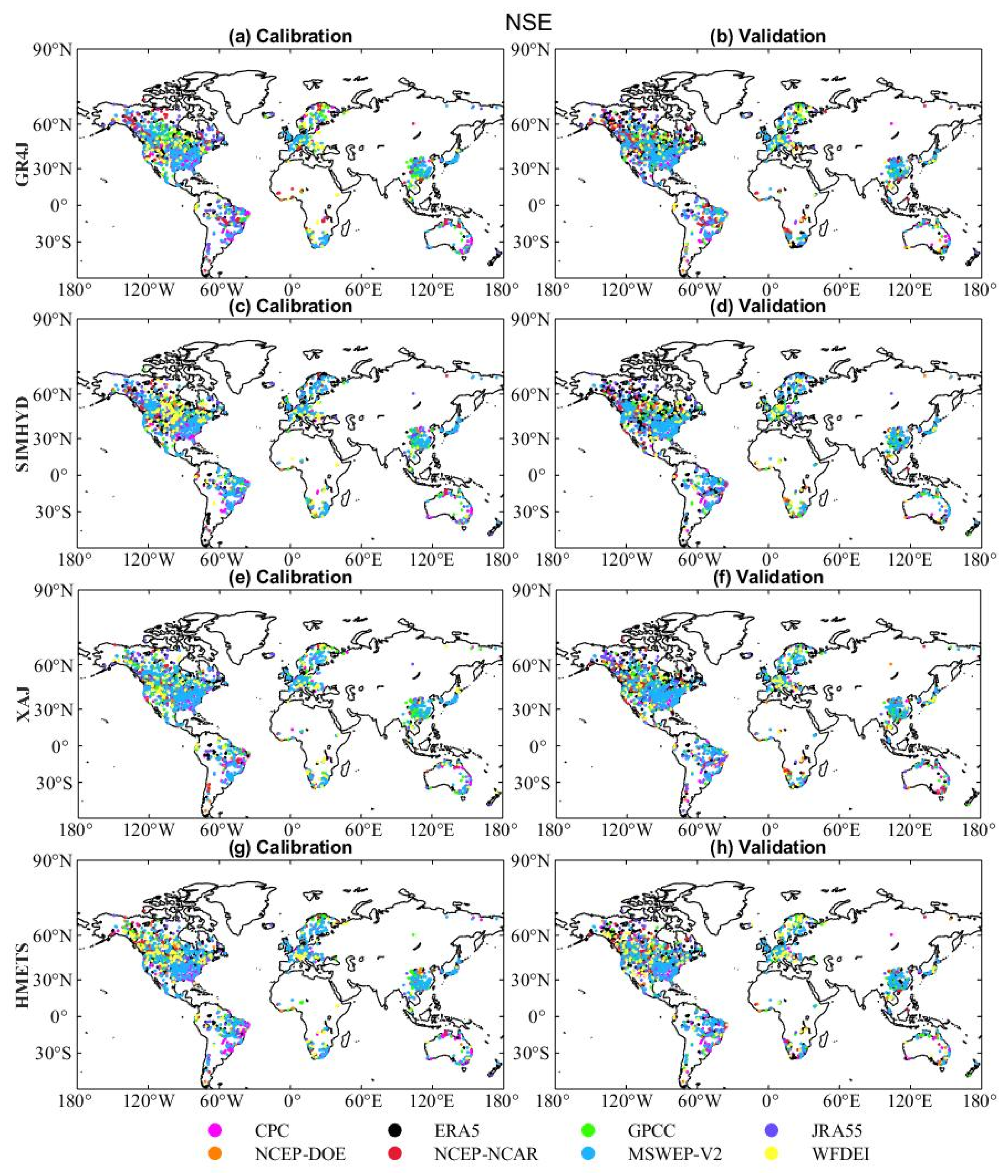
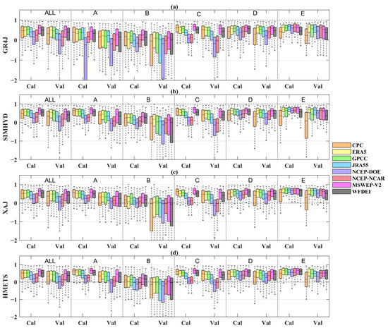
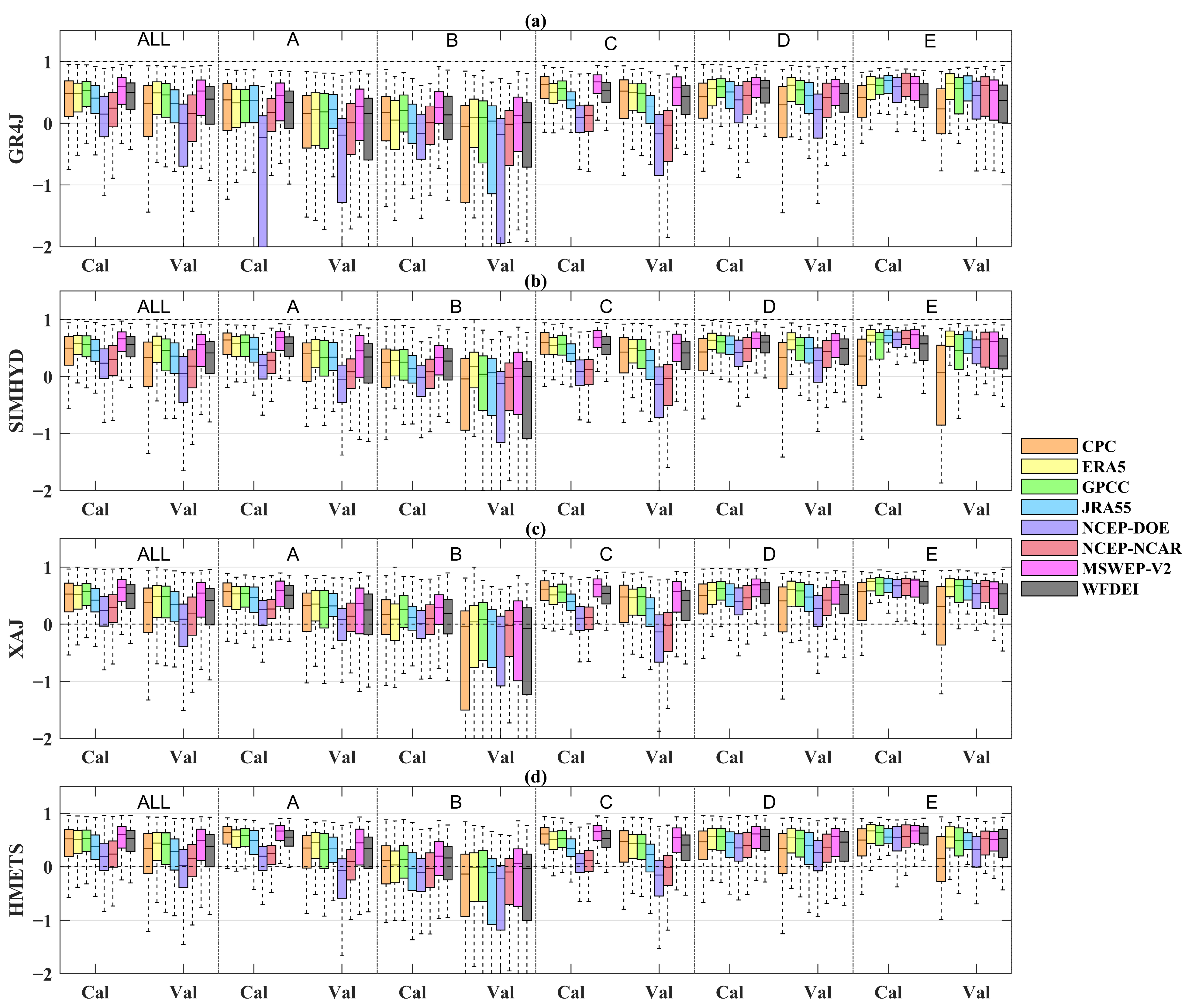
Figure A5.
Boxplots of NSE values of different precipitation datasets for both calibration period (Cal) and validation period (Val) in different climate region ((a) GR4J, (b) SIMHYD, (c) XAJ, (d) HMETS). A, B, C, D and E represent the equatorial (A), arid (B), warm temperate (C), snow (D), and Arctic (E) region, respectively.
References
- Douglas-Mankin, K.R.; Srinivasan, R.; Arnold, J.G. Soil and Water Assessment Tool (SWAT) Model: Current Developments and Applications. Trans. ASABE 2010, 53, 1423–1431. [Google Scholar] [CrossRef]
- Nijssen, B.; O’Donnell, G.M.; Lettenmaier, D.P.; Lohmann, D.; Wood, E.F. Predicting the Discharge of Global Rivers. J. Climate 2001, 14, 3307–3323. [Google Scholar] [CrossRef]
- Wei, Z.; He, X.; Zhang, Y.; Pan, M.; Sheffield, J.; Peng, L.; Yamazaki, D.; Moiz, A.; Liu, Y.; Ikeuchi, K. Identification of uncertainty sources in quasi-global discharge and inundation simulations using satellite-based precipitation products. J. Hydrol. 2020, 589, 125180. [Google Scholar] [CrossRef]
- Ahmed, K.; Shahid, S.; Ali, R.O.; Bin Harun, S.; Wang, X.-j. Evaluation of the performance of gridded precipitation products over Balochistan Province, Pakistan. Desalin. Water Treat. 2017, 79, 73–86. [Google Scholar] [CrossRef]
- Chen, H.; Yong, B.; Shen, Y.; Liu, J.; Hong, Y.; Zhang, J. Comparison analysis of six purely satellite-derived global precipitation estimates. J. Hydrol. 2020, 581, 124376. [Google Scholar] [CrossRef]
- Schneider, U.; Becker, A.; Finger, P.; Meyer-Christoffer, A.; Ziese, M.; Rudolf, B. GPCC’s new land surface precipitation climatology based on quality-controlled in situ data and its role in quantifying the global water cycle. Theor. Appl. Climatol. 2014, 115, 15–40. [Google Scholar] [CrossRef]
- Weedon, G.P.; Balsamo, G.; Bellouin, N.; Gomes, S.; Best, M.J.; Viterbo, P. The WFDEI meteorological forcing data set: WATCH Forcing Data methodology applied to ERA-Interim reanalysis data. Water Resour. Res. 2014, 50, 7505–7514. [Google Scholar] [CrossRef]
- Beck, H.E.; Vergopolan, N.; Pan, M.; Levizzani, V.; van Dijk, A.I.J.M.; Weedon, G.P.; Brocca, L.; Pappenberger, F.; Huffman, G.J.; Wood, E.F. Global-scale evaluation of 22 precipitation datasets using gauge observations and hydrological modeling. Hydrol. Earth Syst. Sci. 2017, 21, 6201–6217. [Google Scholar] [CrossRef]
- Chen, M.; Shi, W.; Xie, P.; Silva, V.B.S.; Kousky, V.E.; Wayne Higgins, R.; Janowiak, J.E. Assessing objective techniques for gauge-based analyses of global daily precipitation. J. Geophys. Res. 2008, 113, D04110. [Google Scholar] [CrossRef]
- Sawunyama, T.; Hughes, D.A. Application of satellite-derived rainfall estimates to extend water resource simulation modelling in South Africa. Water Sa 2018, 34, 1–10. [Google Scholar] [CrossRef]
- Gao, Z.; Tang, G.; Jing, W.; Hou, Z.; Yang, J.; Sun, J. Evaluation of Multiple Satellite, Reanalysis, and Merged Precipitation Products for Hydrological Modeling in the Data-Scarce Tributaries of the Pearl River Basin, China. Remote Sens. 2023, 15, 5349. [Google Scholar] [CrossRef]
- Sun, Q.; Miao, C.; Duan, Q.; Ashouri, H.; Sorooshian, S.; Hsu, K.L. A Review of Global Precipitation Data Sets: Data Sources, Estimation, and Intercomparisons. Rev. Geophys. 2018, 56, 79–107. [Google Scholar] [CrossRef]
- Lei, H.; Zhao, H.; Ao, T. A two-step merging strategy for incorporating multi-source precipitation products and gauge observations using machine learning classification and regression over China. Hydrol. Earth Syst. Sci. 2022, 26, 2969–2995. [Google Scholar] [CrossRef]
- Schamm, K.; Ziese, M.; Becker, A.; Finger, P.; Meyer-Christoffer, A.; Schneider, U.; Schröder, M.; Stender, P. Global gridded precipitation over land: A description of the new GPCC First Guess Daily product. Earth Syst. Sci. Data Discuss. 2013, 6, 435–464. [Google Scholar] [CrossRef]
- Beck, H.E.; Pan, M.; Roy, T.; Weedon, G.P.; Pappenberger, F.; van Dijk, A.I.J.M.; Huffman, G.J.; Adler, R.F.; Wood, E.F. Daily evaluation of 26 precipitation datasets using Stage-IV gauge-radar data for the CONUS. Hydrol. Earth Syst. Sci. 2019, 23, 207–224. [Google Scholar] [CrossRef]
- Shen, Z.; Yong, B.; Gourley, J.; Qi, W.; Lu, D.; Liu, J.; Ren, L.; Hong, Y.; Zhang, J.-y. Recent global performance of the Climate Hazards group Infrared Precipitation (CHIRP) with Stations (CHIRPS). J. Hydrol. 2020, 591, 125284. [Google Scholar] [CrossRef]
- Ashouri, H.; Hsu, K.; Sorooshian, S.; Braithwaite, D.; Knapp, K.; Cecil, L.; Nelson, B.; Prat, O. PERSIANN-CDR: Daily Precipitation Climate Data Record from Multisatellite Observations for Hydrological and Climate Studies. Bull. Am. Meteorol. Soc. 2014, 96, 69–83. [Google Scholar] [CrossRef]
- Huffman, G.; Adler, R.; Bolvin, D.; Gu, G.; Nelkin, E.; Bowman, K.; Hong, Y.; Stocker, E.; Wolff, D. The TRMM Multisatellite Precipitation Analysis (TMPA): Quasi-Global, Multiyear, Combined-Sensor Precipitation Estimates at Fine Scales. J. Hydrometeorol. 2007, 8, 38–55. [Google Scholar] [CrossRef]
- Kobayashi, S.; Ota, Y.; Harada, Y.; Ebita, A.; Moriya, M.; Onoda, H.; Onogi, K.; Kamahori, H.; Kobayashi, C.; Endo, H.; et al. The JRA-55 Reanalysis: General Specifications and Basic Characteristics. J. Meteorol. Soc. Jpn. Ser. II 2015, 93, 5–48. [Google Scholar] [CrossRef]
- Beck, H.E.; Van Dijk, A.I.; Levizzani, V.; Schellekens, J.; Gonzalez Miralles, D.; Martens, B.; De Roo, A. MSWEP: 3-hourly 0.25 global gridded precipitation (1979–2015) by merging gauge, satellite, and reanalysis data. Hydrol. Earth Syst. Sci. 2017, 21, 589–615. [Google Scholar] [CrossRef]
- Xie, P.; Janowiak, J.; Arkin, P.; Adler, R.; Gruber, A.; Ferraro, R.; Huffman, G.; Curtis, S. GPCP Pentad Precipitation Analyses: An Experimental Dataset Based on Gauge Observations and Satellite Estimates. J. Clim. 2003, 16, 2197–2214. [Google Scholar] [CrossRef]
- Duan, Z.; Liu, J.; Tuo, Y.; Chiogna, G.; Disse, M. Evaluation of eight high spatial resolution gridded precipitation products in Adige Basin (Italy) at multiple temporal and spatial scales. Sci. Total Environ. 2016, 573, 1536–1553. [Google Scholar] [CrossRef] [PubMed]
- Tuo, Y.; Duan, Z.; Disse, M.; Chiogna, G. Evaluation of precipitation input for SWAT modeling in Alpine catchment: A case study in the Adige river basin (Italy). Sci. Total Environ. 2016, 573, 66–82. [Google Scholar] [CrossRef]
- Chen, H.; Yong, B.; Kirstetter, P.-E.; Wang, L.; Hong, Y. Global component analysis of errors in three satellite-only global precipitation estimates. Hydrol. Earth Syst. Sci. 2021, 25, 3087–3104. [Google Scholar] [CrossRef]
- Gebremichael, M.; Hirpa, F.A.; Hopson, T. Evaluation of High-Resolution Satellite Precipitation Products over Very Complex Terrain in Ethiopia. J. Appl. Meteorol. Climatol. 2010, 49, 1044–1051. [Google Scholar] [CrossRef]
- Bumke, K.; König-Langlo, G.; Kinzel, J.; Schröder, M. HOAPS and ERA-Interim precipitation over the sea: Validation against shipboard in situ measurements. Atmos. Meas. Tech. 2016, 9, 2409–2423. [Google Scholar] [CrossRef]
- Alijanian, M.; Rakhshandehroo, G.R.; Mishra, A.K.; Dehghani, M. Evaluation of satellite rainfall climatology using CMORPH, PERSIANN-CDR, PERSIANN, TRMM, MSWEP over Iran. Int. J. Climatol. 2017, 37, 4896–4914. [Google Scholar] [CrossRef]
- Hu, X.; Zhou, Z.; Xiong, H.; Gao, Q.; Cao, X.; Yang, X. Inter-comparison of global precipitation data products at the river basin scale. Hydro Res. 2023, 55, 1–16. [Google Scholar] [CrossRef]
- Rivoire, P.; Martius, O.; Naveau, P. A Comparison of Moderate and Extreme ERA-5 Daily Precipitation With Two Observational Data Sets. Earth Space Sci. 2021, 8, e2020EA001633. [Google Scholar] [CrossRef]
- Chen, Y.; Hu, D.; Liu, M.; Shasha, W.; Yufei, D. Spatio-temporal accuracy evaluation of three high-resolution satellite precipitation products in China area. Atmos. Res. 2020, 241, 104952. [Google Scholar] [CrossRef]
- Iqbal, J.; Khan, N.; Shahid, S.; Ullah, S. Evaluation of gridded dataset in estimating extreme precipitations indices in Pakistan. Acta Geophys. 2024, 72, 1–16. [Google Scholar] [CrossRef]
- Lu, J.; Wang, K.; Wu, G.; Mao, Y. Evaluation of Multi-Source Datasets in Characterizing Spatio-Temporal Characteristics of Extreme Precipitation from 2001 to 2019 in China. J. Hydrometeorol. 2024, 25, 515–539. [Google Scholar] [CrossRef]
- Pan, M.; Li, H.; Wood, E. Assessing the skill of satellite-based precipitation estimates in hydrologic applications. Water Resour. Res. 2010, 46, 1–10. [Google Scholar] [CrossRef]
- Martens, B.; Miralles, D.G.; Lievens, H.; van der Schalie, R.; de Jeu, R.A.M.; Fernández-Prieto, D.; Beck, H.E.; Dorigo, W.A.; Verhoest, N.E.C. GLEAM v3: Satellite-based land evaporation and root-zone soil moisture. Geosci. Model Dev. 2017, 10, 1903–1925. [Google Scholar] [CrossRef]
- Gebremichael, M.; Bitew, M.M.; Ghebremichael, L.T.; Bayissa, Y.A. Evaluation of High-Resolution Satellite Rainfall Products through Streamflow Simulation in a Hydrological Modeling of a Small Mountainous Watershed in Ethiopia. J. Hydrometeorol. 2012, 13, 338–350. [Google Scholar] [CrossRef]
- Collischonn, B.; Collischonn, W.; Tucci, C.E.M. Daily hydrological modeling in the Amazon basin using TRMM rainfall estimates. J. Hydrol. 2008, 360, 207–216. [Google Scholar] [CrossRef]
- Falck, A.S.; Maggioni, V.; Tomasella, J.; Vila, D.A.; Diniz, F.L.R. Propagation of satellite precipitation uncertainties through a distributed hydrologic model: A case study in the Tocantins–Araguaia basin in Brazil. J. Hydrol. 2015, 527, 943–957. [Google Scholar] [CrossRef]
- Alexopoulos, M.J.; Müller-Thomy, H.; Nistahl, P.; Šraj, M.; Bezak, N. Validation of precipitation reanalysis products for rainfall-runoff modelling in Slovenia. Hydrol. Earth Syst. Sci. 2023, 27, 2559–2578. [Google Scholar] [CrossRef]
- Sabbaghi, M.; Shahnazari, A.; Soleimanian, E. Evaluation of high-resolution precipitation products (CMORPH-CRT, PERSIANN, and TRMM-3B42RT) and their performances as inputs to the hydrological model. Model. Earth Syst. Environ. 2024, 10, 1–17. [Google Scholar] [CrossRef]
- Maggioni, V.; Meyers, P.C.; Robinson, M.D. A review of merged high-resolution satellite precipitation product accuracy during the Tropical Rainfall Measuring Mission (TRMM) era. J. Hydrometeorol. 2016, 17, 1101–1117. [Google Scholar] [CrossRef]
- Chen, J.; Li, Z.; Li, L.; Wang, J.; Qi, W.; Xu, C.-Y.; Kim, J.-S. Evaluation of Multi-Satellite Precipitation Datasets and Their Error Propagation in Hydrological Modeling in a Monsoon-Prone Region. Remote Sens. 2020, 12, 3550. [Google Scholar] [CrossRef]
- Tang, G.; Zeng, Z.; Long, D.; Guo, X.; Yong, B.; Zhang, W.; Hong, Y. Statistical and Hydrological Comparisons between TRMM and GPM. J. Hydrometeorol. 2016, 17, 121–137. [Google Scholar] [CrossRef]
- Xiang, Y.; Chen, J.; Li, L.; Peng, T.; Yin, Z. Evaluation of Eight Global Precipitation Datasets in Hydrological Modeling. Remote Sens. 2021, 13, 2831. [Google Scholar] [CrossRef]
- Jiang, Q.; Li, W.; Fan, Z.; He, X.; Sun, W.; Chen, S.; Wen, J.; Gao, J.; Wang, J. Evaluation of the ERA5 reanalysis precipitation dataset over Chinese Mainland. J. Hydrol. 2021, 595, 125660. [Google Scholar] [CrossRef]
- Cantoni, E.; Tramblay, Y.; Grimaldi, S.; Salamon, P.; Dakhlaoui, H.; Dezetter, A.; Thiemig, V. Hydrological performance of the ERA5 reanalysis for flood modeling in Tunisia with the LISFLOOD and GR4J models. J. Hydrol. Reg. Stud. 2022, 42, 101169. [Google Scholar] [CrossRef]
- Araghi, A.; Adamowski, J.F. Assessment of 30 gridded precipitation datasets over different climates on a country scale. Earth Sci. Inform. 2024, 17, 1301–1313. [Google Scholar] [CrossRef]
- Fekete, B.M.; Vörösmarty, C.J.; Roads, J.O.; Willmott, C.J. Uncertainties in Precipitation and Their Impacts on Runoff Estimates. J. Climate 2004, 17, 294–304. [Google Scholar] [CrossRef]
- Voisin, N.; Wood, A.W.; Lettenmaier, D.P. Evaluation of Precipitation Products for Global Hydrological Prediction. J. Hydrometeorol. 2008, 9, 388–407. [Google Scholar] [CrossRef]
- Gebrechorkos, S.H.; Leyland, J.; Dadson, S.J.; Cohen, S.; Slater, L.; Wortmann, M.; Ashworth, P.J.; Bennett, G.L.; Boothroyd, R.; Cloke, H.; et al. Global scale evaluation of precipitation datasets for hydrological modelling. Hydrol. Earth Syst. Sci. Discuss. 2023, 2023, 1–33. [Google Scholar] [CrossRef]
- Hersbach, H.; Bell, B.; Berrisford, P.; Hirahara, S.; Horányi, A.; Muñoz Sabater, J.; Nicolas, J.; Peubey, C.; Radu, R.; Schepers, D.; et al. The ERA5 global reanalysis. Q. J. R. Meteorol. Soc. 2020, 146, 1999–2049. [Google Scholar] [CrossRef]
- Kalnay, E.; Kanamitsu, M.; Kistler, R.; Collins, W.; Deaven, D.; Gandin, L.; Iredell, M.; Saha, S.; White, G.; Woollen, J.; et al. The NCEP/NCAR 40-Year Reanalysis Project. Bull. Am. Meteorol. Soc. 1996, 77, 437–472. [Google Scholar] [CrossRef]
- Kanamitsu, M.; Ebisuzaki, W.; Woollen, J.; Yang, S.-K.; Hnilo, J.J.; Fiorino, M.; Potter, G.L. NCEP–DOE AMIP-II Reanalysis (R-2). Bull. Am. Meteorol. Soc. 2002, 83, 1631–1644. [Google Scholar] [CrossRef]
- Du, Y.; Wang, D.; Zhu, J.; Lin, Z.; Zhong, Y. Intercomparison of multiple high-resolution precipitation products over China: Climatology and extremes. Atmos. Res. 2022, 278, 106342. [Google Scholar] [CrossRef]
- Qi, W.-y.; Chen, J.; Li, L.; Xu, C.-Y.; Li, J.; Xiang, Y.; Zhang, S. Regionalization of catchment hydrological model parameters for global water resources simulations. Hydro Res. 2022, 53, 441–466. [Google Scholar] [CrossRef]
- Kottek, M.; Grieser, J.; Beck, C.; Rudolf, B.; Rubel, F. World Map of the Köppen-Geiger climate classification updated. Meteorol. Z. 2006, 15, 259–263. [Google Scholar] [CrossRef]
- Wu, J.; Gao, X.-J. A gridded daily observation dataset over China region and comparison with the other datasets. Chin. J. Geophys. Chin. Ed. 2013, 56, 1102–1111. (In Chinese) [Google Scholar]
- Haylock, M.R.; Hofstra, N.; Klein Tank, A.M.G.; Klok, E.J.; Jones, P.D.; New, M. A European daily high-resolution gridded data set of surface temperature and precipitation for 1950–2006. J. Geophys. Res. 2008, 113, D20119. [Google Scholar] [CrossRef]
- Yang, J. The thin plate spline robust point matching (TPS-RPM) algorithm: A revisit. Pattern Recogn. Lett. 2011, 32, 910–918. [Google Scholar] [CrossRef]
- Burek, P.; Smilovic, M. The use of GRDC gauging stations for calibrating large-scale hydrological models. Earth Syst. Sci. Data 2023, 15, 5617–5629. [Google Scholar] [CrossRef]
- Arsenault, R.; Bazile, R.; Ouellet Dallaire, C.; Brissette, F. CANOPEX: A Canadian hydrometeorological watershed database. Hydrol. Process 2016, 30, 2734–2736. [Google Scholar] [CrossRef]
- Gong, L.; Halldin, S.; Xu, C.Y. Global-scale river routing-an efficient time-delay algorithm based on HydroSHEDS high-resolution hydrography. Hydrol. Process 2011, 25, 1114–1128. [Google Scholar] [CrossRef]
- Perrin, C.; Michel, C.; Andréassian, V. Improvement of a parsimonious model for streamflow simulation. J. Hydrol. 2003, 279, 275–289. [Google Scholar] [CrossRef]
- Zeng, L.; Xiong, L.; Liu, D.; Chen, J.; Kim, J.-S. Improving Parameter Transferability of GR4J Model under Changing Environments Considering Nonstationarity. Water 2019, 11, 2029. [Google Scholar] [CrossRef]
- Valéry, A.; Andréassian, V.; Perrin, C. ‘As simple as possible but not simpler’: What is useful in a temperature-based snow-accounting routine? Part 1—Comparison of six snow accounting routines on 380 catchments. J. Hydrol. 2014, 517, 1166–1175. [Google Scholar] [CrossRef]
- Qi, W.-y.; Chen, J.; Li, L.; Xu, C.-Y.; Xiang, Y.-h.; Zhang, S.-b.; Wang, H.-M. Impact of the number of donor catchments and the efficiency threshold on regionalization performance of hydrological models. J. Hydrol. 2021, 601, 126680. [Google Scholar] [CrossRef]
- Chiew, F.H. Lumped Conceptual Rainfall-Runoff Models and Simple Water Balance Methods: Overview and Applications in Ungauged and Data Limited Regions. Geogr. Compass. 2010, 4, 206–225. [Google Scholar] [CrossRef]
- Chiew, F.H.; Peel, M.C.; Western, A.W. Application and testing of the simple rainfall-runoff model SIMHYD. In Mathematical Models of Small Watershed Hydrology and Applications; Singh, V.P., Frevert, D., Eds.; Water Resources Publications: Littleton, CO, USA, 2002; pp. 335–367. [Google Scholar]
- Zhao, R.-J.; Zuang, Y.; Fang, L.; Liu, X.; Zhang, Q. The Xinanjiang model. In Proceedings of the Oxford Symposium, 15–18 April 1980. Hydrological Forecasting Proceedings Oxford Symposium, IASH 129; International Association of Hydrological Science: Oxfordshire, UK, 1980; pp. 351–356. [Google Scholar]
- Zhao, R.-J. The Xinanjiang model applied in China. J. Hydrol. 1992, 135, 371–381. [Google Scholar]
- Chen, Y.; Shi, P.; Qu, S.; Ji, X.; Zhao, L.; Gou, J.; Mou, S. Integrating XAJ Model with GIUH Based on Nash Model for Rainfall-Runoff Modelling. Water 2019, 11, 772. [Google Scholar] [CrossRef]
- Martel, J.-L.; Demeester, K.; Brissette, F.P.; Arsenault, R.; Poulin, A. HMET: A simple and efficient hydrology model for teaching hydrological modelling, flow forecasting and climate change impacts. Int. J. Eng. Educ. 2017, 33, 1307–1316. [Google Scholar]
- Chen, J.; Brissette, F.P.; Poulin, A.; Leconte, R. Overall uncertainty study of the hydrological impacts of climate change for a Canadian watershed. Water Resour. Res. 2011, 47, W12509. [Google Scholar] [CrossRef]
- Duan, Q.; Gupta, V.K.; Sorooshian, S. Shuffled complex evolution approach for effective and efficient global minimization. J. Optim. Theory Appl. 1993, 76, 501–521. [Google Scholar] [CrossRef]
- Qi, W.; Chen, J.; Xu, C.; Wan, Y. Finding the Optimal Multimodel Averaging Method for Global Hydrological Simulations. Remote Sens. 2021, 13, 2574. [Google Scholar] [CrossRef]
- Gupta, H.V.; Kling, H.; Yilmaz, K.K.; Martinez, G.F. Decomposition of the mean squared error and NSE performance criteria: Implications for improving hydrological modelling. J. Hydrol. 2009, 377, 80–91. [Google Scholar] [CrossRef]
- Perrin, C.; Littlewood, I. A comparative assessment of two rainfall-runoff modelling approaches: GR4J and IHACRES. In Proceedings of the Liblice Conference, IHP-V, Technical Documents in Hydrology n. Liblice, Czech Republic, 22–24 September 1998; Elias, V., Littlewood, I.G., Eds.; UNESCO: Paris, France, 2000; pp. 191–201. [Google Scholar]
- Zhang, H.; Loaiciga, H.; Du, Q.; Sauter, T. Comprehensive Evaluation of Global Precipitation Products and Their Accuracy in Drought Detection in Mainland China. J. Hydrometeorol. 2023, 24, 1907–1937. [Google Scholar] [CrossRef]
- Peng, F.; Zhao, S.; Chen, C.; Cong, D.; Wang, Y.; Hongda, O. Evaluation and comparison of the precipitation detection ability of multiple satellite products in a typical agriculture area of China. Atmos. Res. 2019, 236, 104814. [Google Scholar] [CrossRef]
- Guo, Y.; Yan, X.; Song, S. Spatiotemporal variability of extreme precipitation in east of northwest China and associated large-scale circulation factors. Environ. Sci. Pollut. Res. 2024, 31, 1–17. [Google Scholar] [CrossRef] [PubMed]
- Vis, M.; Knight, R.; Pool, S.; Wolfe, W.; Seibert, J. Model Calibration Criteria for Estimating Ecological Flow Characteristics. Water 2015, 7, 2358–2381. [Google Scholar] [CrossRef]
- Cherchi, A.; Ambrizzi, T.; Behera, S.; Freitas, A.C.V.; Morioka, Y.; Zhou, T. The Response of Subtropical Highs to Climate Change. Curr. Clim. Chang. Rep. 2018, 4, 371–382. [Google Scholar] [CrossRef]
- Svoma, B.; Krahenbuhl, D.; Bush, C.; Malloy, J.; White, J.; Wagner, M.; Pace, M.; DeBiasse, K.; Selover, N.; Balling, R.; et al. Expansion of the northern hemisphere subtropical high pressure belt: Trends and linkages to precipitation and drought. Phys. Geogr. 2013, 34, 174–187. [Google Scholar] [CrossRef]
- Gehne, M.; Hamill, T.M.; Kiladis, G.N.; Trenberth, K.E. Comparison of Global Precipitation Estimates across a Range of Temporal and Spatial Scales. J. Clim. 2016, 29, 7773–7795. [Google Scholar] [CrossRef]
- Islam, S.U.; Déry, S.J. Evaluating uncertainties in modelling the snow hydrology of the Fraser River Basin, British Columbia, Canada. Hydrol. Earth Syst. Sci. 2017, 21, 1827–1847. [Google Scholar] [CrossRef]
- Cattani, E.; Merino, A.; Levizzani, V. Evaluation of Monthly Satellite-Derived Precipitation Products over East Africa. J. Hydrometeorol. 2016, 17, 2555–2573. [Google Scholar] [CrossRef]
- Wang, Y.; Sun, W.; Huai, B.; Wang, Y.; Ji, K.; Yang, X.; Du, W.; Qin, X.; Wang, L. Comparison and evaluation of the performance of reanalysis datasets for compound extreme temperature and precipitation events in the Qilian Mountains. Atmos. Res. 2024, 304, 107375. [Google Scholar] [CrossRef]
- Pfeifroth, U.; Müller, R.; Ahrens, B. Evaluation of Satellite-Based and Reanalysis Precipitation Data in the Tropical Pacific. J. Appl. Meteorol. Climatol. 2013, 52, 634–644. [Google Scholar] [CrossRef]
- Blarzino, G.; Castanet, L.; Luini, L.; Capsoni, C.; Martellucci, A. Development of a new global rainfall rate model based on ERA40, TRMM, GPCC and GPCP products. In Proceedings of the Antennas and Propagation, 2009, EuCAP 2009, 3rd European Conference, Berlin, Germany, 23–27 March 2009. [Google Scholar]
- Widén-Nilsson, E.; Halldin, S.; Xu, C.-y. Global water-balance modelling with WASMOD-M: Parameter estimation and regionalisation. J. Hydrol. 2007, 340, 105–118. [Google Scholar] [CrossRef]
- Beck, H.E.; van Dijk, A.I.J.M.; de Roo, A.; Miralles, D.G.; McVicar, T.R.; Schellekens, J.; Bruijnzeel, L.A. Global-scale regionalization of hydrologic model parameters. Water Resour. Res. 2016, 52, 3599–3622. [Google Scholar] [CrossRef]
- Ghebrehiwot, A.A.; Kozlov, D.V. Hydrological modelling for ungauged basins of arid and semi-arid regions: Review. Vestnik MGSU 2019, 14, 1023–1036. [Google Scholar] [CrossRef]
- Peña-Arancibia, J.L.; van Dijk, A.I.J.M.; Mulligan, M.; Bruijnzeel, L.A. The role of climatic and terrain attributes in estimating baseflow recession in tropical catchments. Hydrol. Earth Syst. Sci. 2010, 14, 2193–2205. [Google Scholar] [CrossRef]
- Behrangi, A.; Wen, Y. On the Spatial and Temporal Sampling Errors of Remotely Sensed Precipitation Products. Remote Sens. 2017, 9, 1127. [Google Scholar] [CrossRef]
- Xu, C.-Y.; Chen, H.; Guo, S. Hydrological Modeling in a Changing Environment: Issues and Challenges. J. Water Resour. Res. 2013, 2, 85–95. [Google Scholar] [CrossRef]


Disclaimer/Publisher’s Note: The statements, opinions and data contained in all publications are solely those of the individual author(s) and contributor(s) and not of MDPI and/or the editor(s). MDPI and/or the editor(s) disclaim responsibility for any injury to people or property resulting from any ideas, methods, instructions or products referred to in the content. |
© 2024 by the authors. Licensee MDPI, Basel, Switzerland. This article is an open access article distributed under the terms and conditions of the Creative Commons Attribution (CC BY) license (https://creativecommons.org/licenses/by/4.0/).