Abstract
Hydrochemical analysis is crucial for understanding soil and water composition dynamics in coastal aquifers. This study presents a novel framework for the comprehensive assessment of groundwater quality, integrating multivariate analysis and hydrochemical techniques. It comprises seven stages aimed at characterizing physicochemical properties, identifying water constituents, elucidating dominant mechanisms in water composition, evaluating ion exchange processes, analyzing spatial distribution of components, identifying impacting processes, and assessing drinking water quality. The framework was applied to the coastal unconfined Arroyo Grande aquifer in Cartagena, Colombia. Fifteen points were sampled, assessing physicochemical parameters such as total hardness, alkalinity, pH, temperature, electrical conductivity, anions, cations, among others. Findings reveal the presence of dominant anions including bicarbonate, chloride, and sulfate, with relevant variations observed between the dry and wet season, with manganese and iron surpassing WHO drinking water standards. The prevalence of these constituents has been attributed to mineral dissolution, ion exchange, salinization due to seawater intrusion, and anthropogenic contamination. Over 50% of samples in both seasons fail to meet freshwater drinking standards due to elevated dissolved mineral concentrations in groundwater. These findings provide insights for sustainable management and mitigation strategies, and the systematic approach enables researchers to identify key factors influencing water composition.
1. Introduction
Groundwater is a vital resource necessary to meet the increasing demand for freshwater worldwide. Nevertheless, knowledge of the subterranean systems and their proper management is usually limited. Regions with groundwater governance key deficiencies, such as, low political commitment, limited integration of science-based groundwater understanding, and limited awareness of long-term groundwater risks, usually have significant gaps in information about the resource [1,2]. Furthermore, the pressures of human activities and climate change continue to impact groundwater quality, posing a threat to its sustainability [3,4].
In recent decades, research has increasingly focused on improving the study of unconfined coastal aquifers, particularly in regions where the effects of climate change are more pronounced, influencing water availability and quality [5]. These aquifers exhibit unique characteristics due to their geology. They are also vulnerable to external forces, such as changing relative sea levels, overexploitation, salinization, and the vertical infiltration of wastewater [3,5].
Coastal aquifers of the Caribbean region of Colombia have evidenced that saltwater intrusion affects the chemical composition of wells located near the beach, and this composition can variate with the depth of the water sample [6,7]. The Arroyo Grande aquifer is vulnerable to various sources of contamination, and previous studies have shown detriment of the water quality [8] and increase in the relative sea level [9].
In the past decade, the region brought special attention to the Arroyo Grande aquifer, considering that it has the potential to supply coastal communities [10,11], places where there is a lack of reliable access to freshwater and currently dependent on the intermittent delivery of freshwater by tank trucks from the city of Cartagena, Colombia. The lack of integrated studies on the water quality of this aquifer limits the understanding and the design of adequate solutions that guarantee its sustainability and adequate governance [12].
Various tools have been applied for quantifying water quality in Colombia and worldwide, including hydrochemical diagrams and indices [2,6,7,8,9,10,11,12,13]. The water quality index (WQI) is a widely adopted mathematical tool for assessing overall water quality at specific locations and times. The WQI has been applied in numerous studies globally, including in regions such as various Indian states, Uttar Pradesh (India), Tefenni plain (Burdur/Turkey), Kadey (East-Cameroon), among others [14,15]. Multivariate statistical tools, specifically principal component analysis (Factor Analysis), aid in interpreting the analytical results of hydrogeochemical studies. They contribute to identifying sources of water quality parameters and understanding the geochemical evolution of groundwater in aquifers [13,16,17].
Although these tools do not establish direct cause-and-effect relationships, they provide valuable information that can be used to infer such relationships. Principal component analysis is effective in identifying associations among different variables and reducing data dimensionality. These assessments have been applied successfully in numerous studies. However, they have been commonly explored using a fragmented approach, employing tools and techniques separately. These can result in difficulties in synthesizing the results, potential oversights, inefficient resource utilization, limited holistic insights, and challenges in decision-making [18,19]. Achieving groundwater sustainability demands a comprehensive understanding of aquifer dynamics and the primary factors influencing water chemistry.
This manuscript introduces a novel framework for comprehensive groundwater quality assessment, providing a holistic view of groundwater quality. The proposed framework encompasses seven sequential steps. First, physicochemical characterization involves extensive data collection through monitoring databases and sampling campaigns, followed by careful analysis to capture seasonal variations in groundwater composition linked to rainfall patterns. Subsequently, the identification of water constituents and types employs laboratory analysis and graphical representations, such as Schoeller plots and Piper diagrams to identify minor ions crucial for quality assessment, in addition to determining dominant mechanisms in water composition, through the analysis of total dissolved solids (TDS), chloride, and bicarbonate levels.
The evaluation of ion exchange processes integrates scatter diagrams and the CAI index, particularly valuable in rock–water interaction scenarios. Spatial distribution analysis, including ion concentration mapping, generates isoline maps highlighting parameters essential for assessing drinking water quality. Multivariate statistical analysis, such as principal component analysis (PCA), identifies interrelated chemical parameters and impacts on water composition, reinforcing insights from earlier steps. Lastly, drinking water quality assessment via the water quality index (WQI) integrates findings from spatial analysis and process identification, culminating in a holistic evaluation of groundwater suitability for consumption.
By integrating advanced data analysis techniques and hydrochemical methods, this framework enhances our understanding of the intricate processes influencing groundwater composition and quality. The framework’s effectiveness is demonstrated through the Arroyo Grande case study and the particularities of its hydrogeological settings.
In this study, hydrochemical diagrams and indices were selected to identify the main characteristics of the chemical composition of groundwater in the Arroyo Grande coastal aquifer. By integrating advanced analytical tools and data-driven methodologies, this framework contributes to advancing scientific knowledge and informs evidence-based decision-making for the sustainable management of the Arroyo Grande aquifer.
2. Review of Hydrochemical Studies of Coastal Aquifers
A review was conducted to assess recent advances in hydrochemical analyses of coastal aquifers, highlighting several common aspects. These include the aquifer’s location, geological characteristics, seasonal climate conditions during the study period, classification of water types based on predominant anion and cations, temporary ion analyses identifying dominant ions, prevalent hydrochemical processes, and applied hydrochemical analyses. The selected studies encompassed coastal aquifers situated in various regions: the Arabian Sea southeast of India in Udupi district [20]; the Mediterranean Sea in the Gaza Strip, Palestine [21]; the South China Sea, Malaysia [22]; the Gulf of Guinea in Lagos, Nigeria [23]; the Mediterranean Sea in various locations including Tunisia (Jerba Island), Libya (Tripoli), Algeria (Nador plain), Morocco (Bou Areg), Italy (Sardinia), and Egypt (Baghoush area) [24]; the Caribbean Sea coast in Quintana Roo, Mexico [25]; the Recife Sea coast, Brazil [17]; and the Caribbean Sea coast in the Gulf of Morrosquillo, Colombia [6]. Relevant findings are summarized in Table S1 (Supplementary Material).
A comparison was made among parameters considered crucial for identifying geogenic and anthropogenic contamination processes, such as chlorides (Cl−), total dissolved solids (TDS), and nitrates (NO3−). The majority of the reviewed aquifers in Appendix A Table A1 consisted of sedimentary rocks and deposits. Ions such as Ca2+, Na+, HCO3−, and SO42− show high significance to the groundwater composition due to rock–water interactions, mineral dissolution and ion exchange, and seawater intrusion [21,25].
According to the data shown in Appendix A Table A1, the prevalence of chloride anion (Cl−) is linked to systems experiencing marine intrusion, which is increasingly relevant in coastal areas. By 2019, at least 501 coastal cities worldwide reported marine intrusion crises, with population density being a primary contributing factor [26]. For example, in the coastal aquifer of southwestern India [20], the highest chloride anion concentration observed was 17,402 mg/L during the pre-monsoon period characterized by low rainfall. Similarly, coastal aquifers along the Mediterranean Sea, in both in Europe and Africa, exhibit elevated average chloride concentrations (Tunisia: 1951 mg/L; Libya: 577 mg/L; Algeria: 770 mg/L; Morocco: 1828 mg/L; Italy: 595 mg/L; Egypt: 1987 mg/L) [24], highlighting marine intrusion as the primary agent of salinization in these systems.
Elevated nitrate anion levels can be attributed to anthropogenic activities such as wastewater and industrial discharge, as well as fertilizer and pesticide use [17,27]. Concentrations exceeding 10 mg/L are considered indicative of anthropogenic contamination in groundwater [20]. The World Health Organization (WHO) has established a threshold of 50 mg/L for nitrate (NO3−) content as a guideline of groundwater quality [28]. Analyses conducted during different climatic seasons showed higher nitrate (NO3−) concentrations during the rainy season. For instance, in the aquifer of the Recife Metropolitan Region (Brazil), maximum recorded values reached up to 207.6 mg/L [17]. In the Lagos Aquifer (Nigeria), maximum values of 108.7 mg/L were reported during the rainy season [23], while the aquifer in the southern zone of Quintana Roo (Mexico) [25] recorded a maximum value of 7.93 mg/L during the same period. Observations from the Gaza aquifer (Palestine) and Mediterranean coastal aquifers [24] recorded maximum values above 100 mg/L, with the aquifer in the Baghoush area (Egypt) reaching the highest value at 7142 mg/L.
Despite the varying factors affecting these systems, common aspects can be identified in the processes determining groundwater composition and the pollution issues they face. Table 1 summarized the majority ions, the dominant hydrochemical processes, the type of aquifers, and the applied hydrochemical analysis for the studies revised in Table A1. From the review and Table 1, it is evidenced that the geology and hydraulic connectivity with the sea in coastal aquifer systems have a significant impact on groundwater composition.

Table 1.
Main characteristics of the reviewed studies in coastal aquifers.
3. Methods and Materials
3.1. Study Area
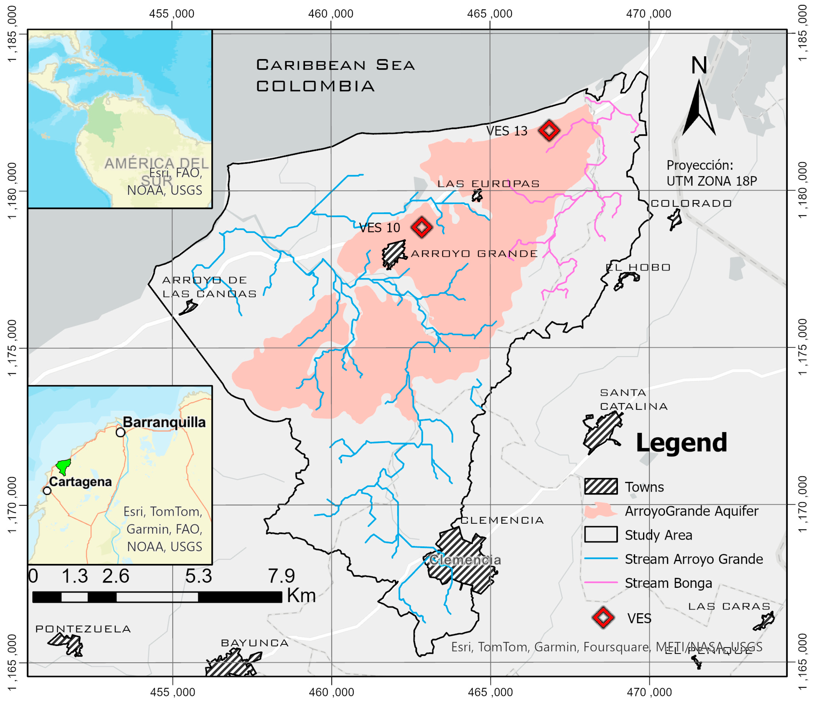
The Arroyo Grande hydrogeological unit and its corresponding basin are situated in the Colombian Caribbean region, north of Cartagena. The aquifer lies along a coastal strip and encompasses towns within the tourist district of Cartagena, as well as the municipalities of Santa Catalina and Clemencia. It is part of the coastal hydrogeological province PC1—Sinú San Jacinto. The study area covers approximately 143 km2 (see Figure 1), bounded by coordinates X(m): 454,559.081 to 468,442.630 and coordinates Y(m): 1,181,790.930 and 1,165,642.759 in zone UTM 18N. This hydrogeological formation is of critical importance to the coastal region, serving as the primary water source for 36,255 inhabitants from the nearby communities.
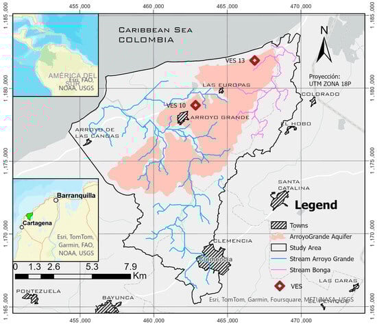
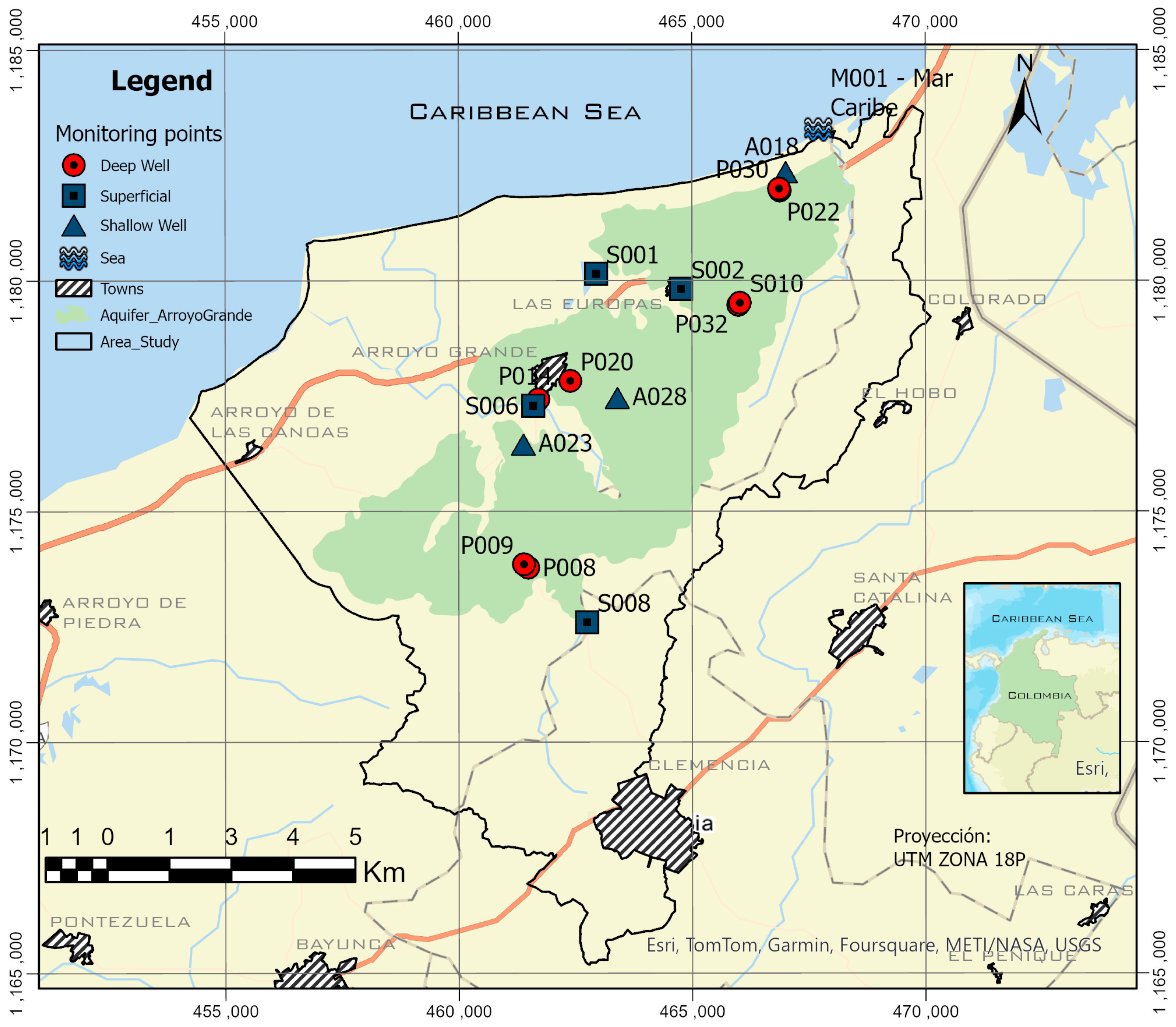
Figure 1.
Location of study area in the northern area of Colombia. The area in pink represents the Arroyo Grande aquifer, and the zone delineated in black is the area of this study. The blue line (Arroyo Grande stream) and the pink line (Bonga stream) show the two main streams that serve the aquifer, and the red diamonds show the location of the vertical electrical soundings (VESs).
According to records from meteorological stations in the area, the multiannual average rainfall corresponds to 1235.37 mm/year, with an estimated average maximum temperature of 30.26 °C [29]. The precipitation is distributed throughout the year in two climatic periods: a dry period with average monthly rainfall ranging from 0 to 60 mm, considered to be the dry season, and a rainy period with average monthly rainfall ranging from 120 to 250 mm, considered the wet season [8,30]. The dry and wet season usually last six months each; however, during periods of El Niño Southern Oscillation (ENSO), the seasons can last longer than normal and generate drastic consequences to the water quality of surface and subterranean water resources [3,31].
The hydrography of the area includes various water sources such as the Caribbean Sea, lakes, springs, and streams. The Arroyo Grande basin, of the same name as the aquifer, has an extension of 96 km2, and it is the most important basin in the area [32].
Geology and Hydrogeology
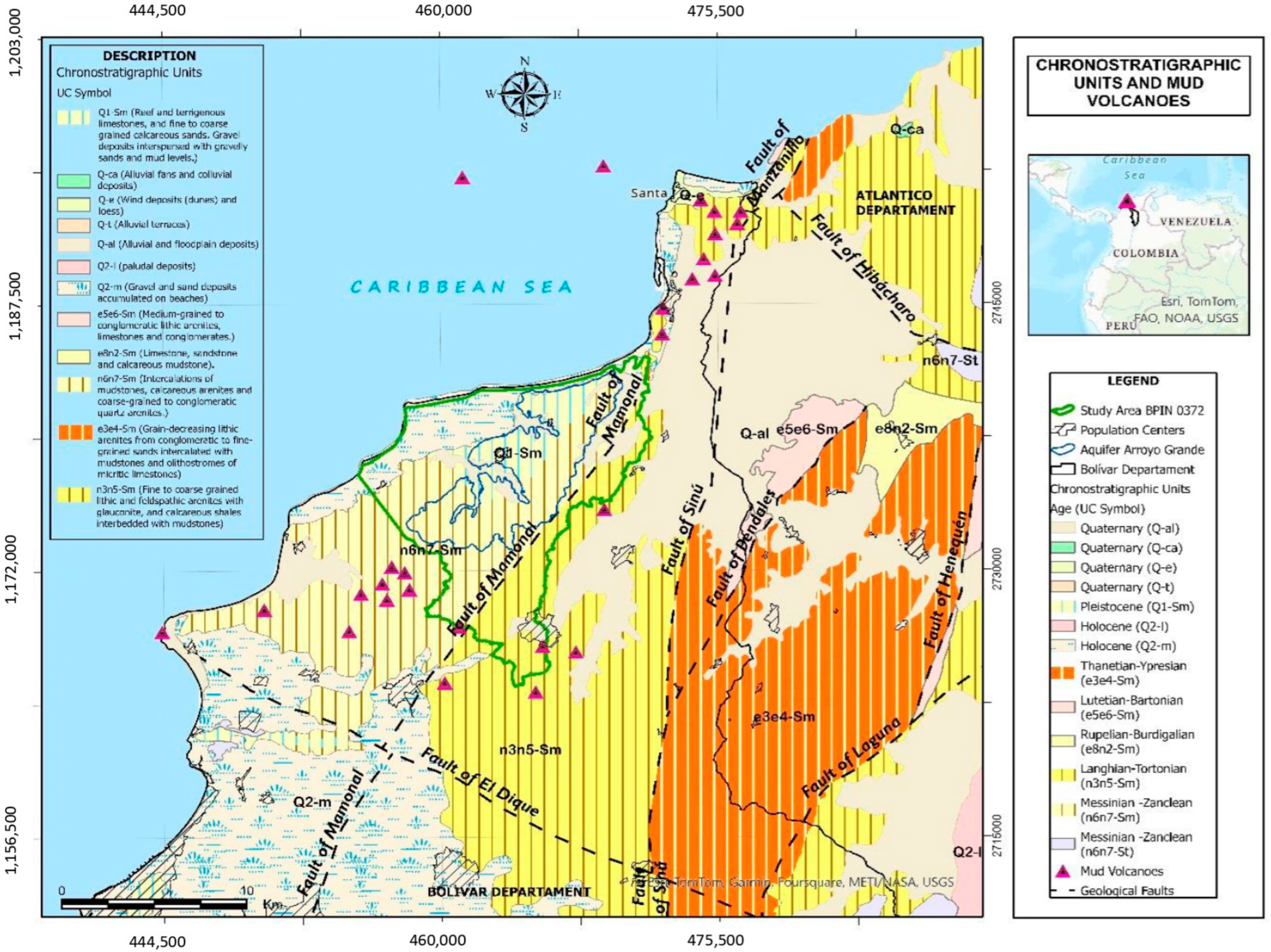
The area is composed of sedimentary rocks that are part of the Sinú belt or Turbaco tectonic block. These rocks include the Arjona Formation from the Oligocene–Miocene Epoch of the Cenozoic, the Bayunca Formation from the Miocene–Pliocene Epoch of the Cenozoic, and the Arroyo Grande and La Popa Formations from the Pleistocene Epoch of the Cenozoic [33]. The Arroyo Grande Formation (Q1-Sm) (refer to Figure 2) is considered a young unit due to the limited consolidation of its deposits, primarily consisting of gravel and sand deposits found in Arroyo Grande township, located northwest of the Cartagena district [34]. Figure 2 was developed by the authors using ArcGisPro 11.0. The layers of geology and the geological data used for this map are open data from the Geologic map of Colombia 2023, available at the Colombian Geologic Survey [35].
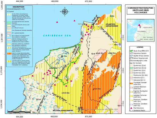
Figure 2.
Chronostratigraphic geological units in the study area surrounding the Arroyo Grande aquifer. The area delineated in green refers to the area selected for this study, and the area delineated in blue is the Arroyo Grande formation.
The stratigraphic columns of greatest reference correspond to the Balastrera section of Arroyo Grande, featuring a base composed of pebble gravel and imbricated grains, with conglomeratic sandstones and sandy conglomerates. The upper part consists of slightly coarse-grained conglomeratic sandstones in thick layers, with the presence of lenticular layers of mudstones in the lower part. The Turbaná–Turbaco section comprises reddish and yellowish claystone in the lower part, interspersed with fine-grained quartz sandstones. The Pasacaballos section is mainly characterized by fine-grained, reddish quartz sandstones alternating with intercalations of gray claystone [34].
The Arroyo Grande aquifer (aT) hydrogeological unit belongs to the PCA1 Sinú San Jacinto hydrogeological province [32]. It is an unconfined regional aquifer with continuous extension. The hydraulic conductivity values range between 1.0 m/day and 3.5 m/day, and the coefficient of storage ranges from 5.0 × 10⁻¹ to 3.0 × 10⁻⁷. Extraction flow rates can vary between 2 and 35 L/s [8]. Vertical Electrical Sounding (VES) previously conducted in the aquifer exploitation zones allowed the depiction of the lithological columns presented in Figure 3. The lithology describes layers of sediment that vary from sand and gravel from the topsoil to approximately 20 m in both VES. VES 13 shows a large layer of sand from 2 m to 12 m followed by sand and gravel. Layers saturated with fresh water lie at depths ranging from 20 to 100 m (see Figure 3) [36].
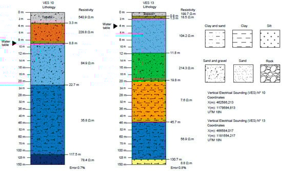
Figure 3.
Lithological columns derived from Vertical Electrical Soundings (VESs) in the area of study [37]. The resistivity of each stratum is presented, alongside the VES location coordinates and the location of the water table.
These layers consist predominantly of coarse sands exhibiting resistivities exceeding 100 Ω.m, while the surface layers are characterized by granular sand type material and saturated silt as detailed in Appendix A Table A2 and Table A3.
3.2. Proposed Integrated Framework
Table 2 presents the proposed integrated framework for analyzing groundwater quality and the relationship between rock dewatering and groundwater composition. This framework outlines the necessary steps for a comprehensive analysis of the physicochemical composition of groundwater and the associated processes, with a specific focus on rock–water interactions. Based on the findings from Appendix A Table A1 and the conducted review, it is evident that the main characteristics of groundwater are of geogenic origin. The framework delineates essential information, applicable techniques (including statistics, graphics, and geospatial analysis), relevant considerations at each stage, and their interrelationships.
Table 2.
Framework to evaluate groundwater quality and the relationship between rock weathering and groundwater hydrogeochemistry.
To apply the framework effectively, it is necessary to preliminarily identify the target aquifer for study, delineate the study area, and develop an inventory of groundwater infrastructure along with surface water sources connected to the aquifer.
The initial step involves conducting physicochemical characterization of water samples following a defined sampling program within the monitoring network. Laboratory analysis results are subjected to statistical and graphical methods to identify key components, water types, and indications of water composition origin. Graphical techniques are employed to determine relevant mechanisms influencing water composition, including rock–water interaction, rainfall, and evaporation. Given the critical role of ion exchange processes in groundwater composition, their evaluation is integral within this framework.
During the next stage, a multivariate statistical analysis is applied to identify processes with the most significant impact on water composition and their interaction with chemical parameters.
The final step entails assessing water quality and establishing the state of drinking water quality based on its composition and related processes. This framework was applied to analyze the hydrogeological characteristics of the Arroyo Grande aquifer in Colombia.
3.2.1. Physicochemical Characterization
A comprehensive survey of the study area was conducted, accompanied by an inventory of water points. A total of 10 groundwater points and 5 surface water points were strategically selected for further analysis based on criteria such as spatial representativeness, accessibility, availability of infrastructure, and cooperation of operators and owners [38]. Georeferencing was performed for all fifteen points, and a detailed map was generated using ArcGIS 11.0 software as presented in Figure 4.
Sampling was performed following the recommendations of the standard methods for examination of water and wastewater [39] and the Colombian Technical Standard [40]. Samples were collected through the well pumping system or directly in the different surface water bodies and then stored and preserved, following the recommendations of the IDEAM and the standard methods for examination of water and wastewater [39].
Temperature, pH, conductivity, salinity, dissolved oxygen, oxidation–reduction potential (ORP), and total dissolved solids (TDS) were measured in situ. Samples to determine the rest of the variables were packaged and preserved for transport to the laboratory, following the methodology of the APHA, AWWA, WEF in the standard methods for the examination of water and wastewater [39].
Two sampling campaigns were conducted: the first during the dry season (April 2022) and the second during the rainy season (July 2022), adhering to established regulations and technical guidelines for water monitoring. On-site measurements were conducted using the HI9829 multiparameter equipment from HANNA Instruments, which facilitated the measurement of various parameters including pH, temperature, electrical conductivity, salinity, dissolved oxygen, ORP (oxidation–reduction potential), and TDS (total dissolved solids). Additionally, water samples ranging from 0.25 to 2 L were collected in both plastic and glass containers. These samples were carefully preserved, stored, and transferred to certified laboratories for the analysis.
The samples were analyzed by the Aguas de Cartagena SA ESP water quality laboratory, accredited by ONAC ISO/IEC 17025:2005, and the SGS COLOMBIA SAS laboratory, accredited by IDEAM resolution No. 0186 of 8 March 2021. A comprehensive range of chemical parameters were analyzed, encompassing HCO3−, SO42−, Cl−, NO2−, NO3−, PO4, Ca2+, Mg2+, Na+, Fe+, NH4+, Mn+, P, As, Hg, Pb, Se, NKT, total hardness, and alkalinity. Various analytical methods such as colorimetric, volumetric, ionic chromatography, and spectrophotometry were employed for these analyses [39]. The analytical errors are included in Appendix A Table A4.
The anions were measured by ionic chromatography, following the regulations of U.S. EPA 300:0 [41], and cation concentrations were measured following the ICP/MS method (standard in water chemistry) [42]. HCO3 was calculated using the volumetric method following the standard method SM 2320 B.
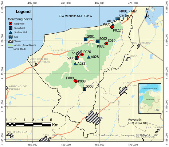
Figure 4.
Location and code of sampling points. Deep well refers to a mechanically drilled structure with diameters typically ranging from 0.15 to 0.3 m and depths exceeding 30 m (P008: 77 m, P009: 80 m, P014: 80.5 m, P020: 69 m, P022: 72 m P030: 76 m, P032: 72 m). Shallow well refers to a large diameter structure built manually, which reaches the water table and is deepened below it to capture groundwater; it does not usually exceed 30 m deep (A018: 4 m, A023: 12 m A028: 23 m) [43].
3.2.2. Identification of Water Constituents and Types of Water
Descriptive Statistics
Upon receiving and tabulating laboratory results, statistical calculations for position, centralization, dispersion, and box-and-whisker plots were performed using JASP 0.15 software [44]. Initial analysis was focused on key water components and their average concentrations across different sampling points [17,45].
Hydrochemical Diagrams and Indices
To identify water types and underlying chemical processes, hydrochemical diagrams including Piper, Gibbs, Schoeller, and scatter plots of ionic ratios along with the CAI index were generated using AQUACHEM 11.0 software [37]. These diagrams utilize major ion concentrations to detect element sources and evolution patterns.
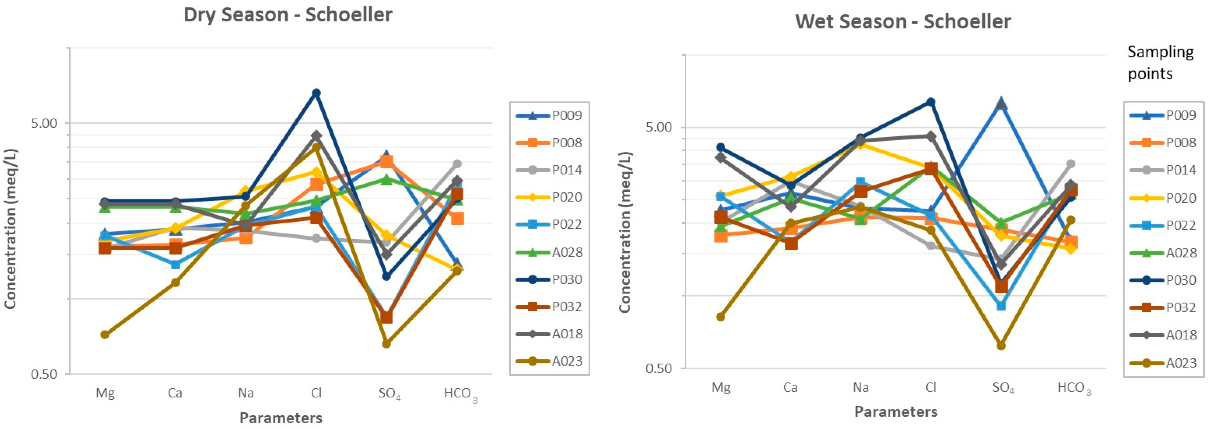
Schoeller Plot
The Schoeller plot was used to determine the order of abundance of anions and cations in groundwater, plotting average ion concentrations from the two sampling campaigns on a semi-logarithmic scale [46].
Piper Diagram
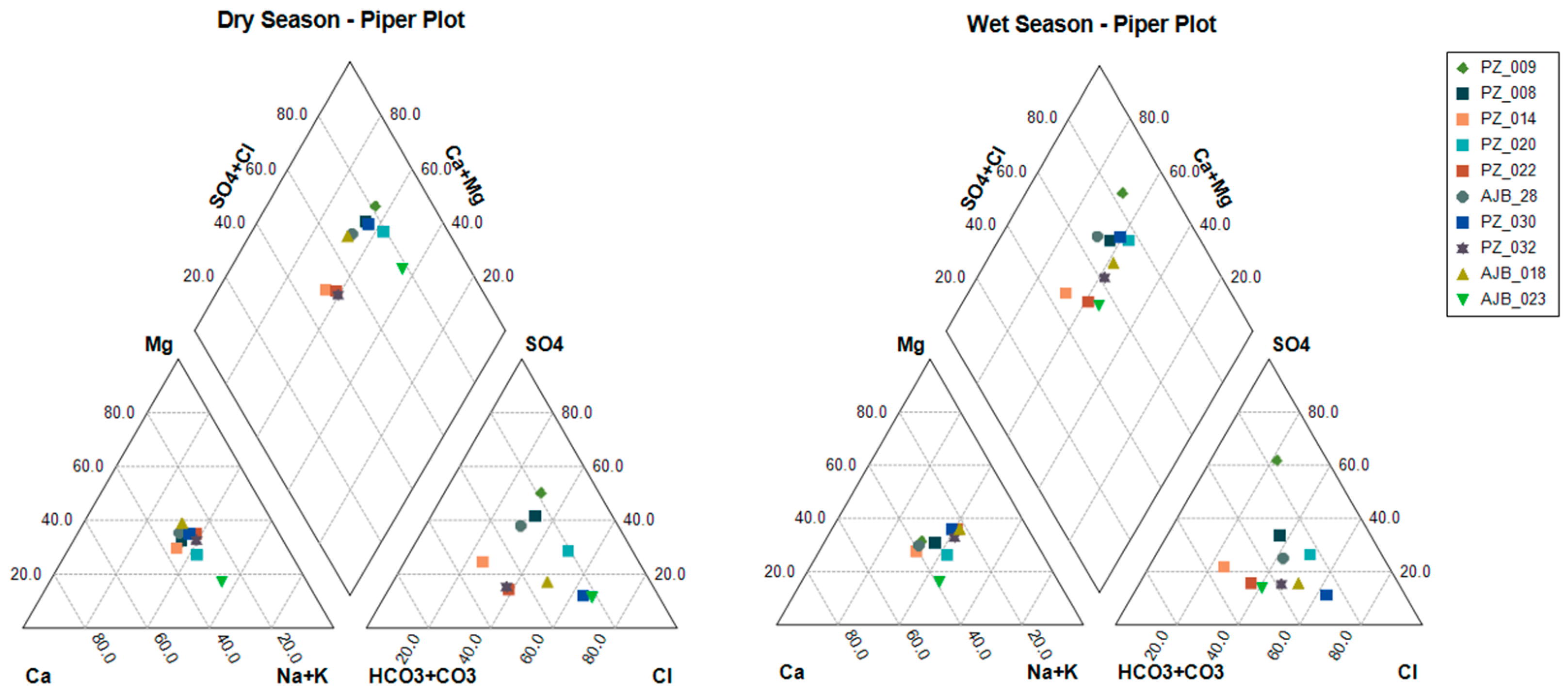
Water types and associated chemical processes were identified using the Piper diagram, which represents major anions (HCO3−, SO42−, Cl−) and cations (Ca2+, Mg2+, Na+, K+) in two equilateral triangles. The intersection of plotted points within a central diamond establishes different water types based on their chemical composition [19,21]. This diagram is widely used in hydrochemical analysis and represents a relatively easy and applicable tool for the study of groundwater; however, it has the disadvantage that it is difficult to show concentration values.
3.2.3. Identification of Dominant Mechanisms in Water Composition
Gibbs Plot
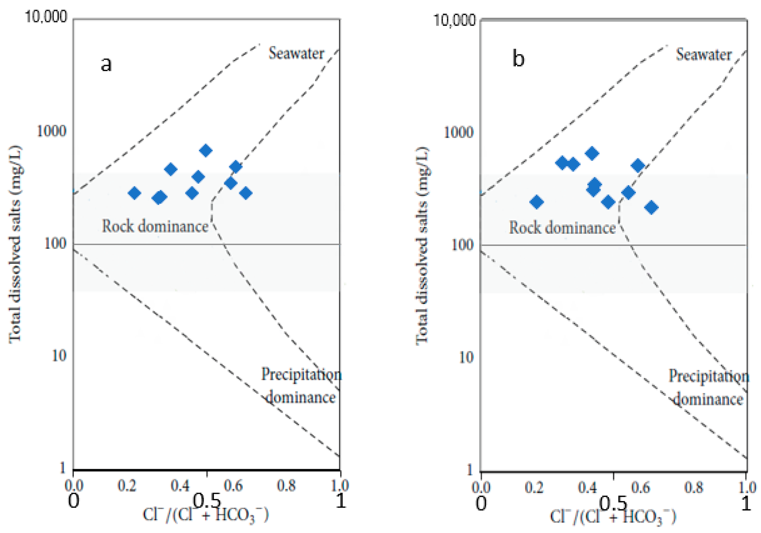
The Gibbs diagram correlates total dissolved solids (TDS) with the ratio of chlorides to bicarbonates (RI) to identify dominant mechanisms influencing water composition, such as rock–water interaction, rainfall, and evaporation, as described in Equation (1) [22,47]. According to this diagram, rainwater typically exhibits high concentrations of NaCl due to its marine origin and low TDS concentrations. In contrast, mineral dissolution processes resulting from rock–water contact increase the TDS content, while evaporation and runoff can lead an increase in both TDS and NaCl concentrations [17].
3.2.4. Evaluation of Ion Exchange Processes
Scatter Diagrams of Ionic Ratios
Ion exchange processes (IEPs) were evaluated using dispersion diagrams of ionic relations. One such diagram plots the sum of cations (Ca2+ and Mg2+) against the sum of anions (HCO3− and SO42−), with cations on the X-axis and anions on the Y-axis. Points near a 1:1 slope indicate mineral dissolution processes, while deviations above and below the line suggest direct and reverse ion exchange processes, respectively [46,47].
Salinization processes associated with seawater mixing were analyzed using electrical conductivity (EC) and chlorides (Cl−) [24].
CAI Index
The chloro-alkaline indices (CAI) were used to identify softening or hardening processes in groundwater based on specific variables defined in Equations (2) and (3) [2,23].
3.2.5. Identification of Processes Impacting Water Composition and Interrelationship between Chemical Parameters
Multivariate Statistical Analysis
The Statgraphics 19 software was employed to perform the principal component analysis (PCA). Prior to conducting the analysis, the variables were standardized to achieve a normal distribution, using Equation (4) [37,48].
where , , and are the standardized value of sample j for parameter i, original value of sample i in parameter j, and standard deviation of parameter j, respectively.
3.2.6. Drinking Water Quality Assessment
The water quality index (WQI) was applied to assess the quality of groundwater based on the concentration of certain physicochemical parameters [49,50,51]. Such parameters were identified and assigned weights based on their potential impact on human health, particularly in the context of drinking water [52,53].
Table 3 presents the assigned weights () to physicochemical parameters ranging between 1 and 5. The relative weight () was calculated using Equation (5), where n is the total number of parameters. Subsequently, the quality rating ) is calculated based on the concentration of each parameter () and its standard () as established by the drinking water standards of the World Health Organization (WHO) [54] (Equation (6)). Finally, the WQI is determined by summing the sub-index (SI) calculated for each parameter using Equations (7) and (8). Based on the results of the WQI, the quality status is assessed for each sample according to the ranges specified in Table 4 [52].
Table 3.
Weight assignment to physicochemical parameters.
Table 4.
WQI range, status, and possible usage of the water sample [52].
4. Results and Discussion
The data obtained from the field measurements provided a preliminary identification and general overview of the environmental conditions and physical characteristics of the water in the study area. The descriptive statistics presented in Table 5 show that the average water temperature at the sampled points during both campaigns correlates with the average maximum ambient temperature of 30.26 °C, with an average temperature of 29.6 °C for the first campaign and 29.36 °C for the second campaign.
Table 5.
Descriptive statistics of parameters measured on site at 15 sampling points—Campaign No. 1 (dry season)–Campaign No. 2 (wet season).
The highest temperature values recorded correspond to surface waters, while groundwater shows similar temperature during dry and wet seasons. These conditions can be attributed to the shallow nature of the aquifer. In studies of aquifers deeper than 700 m, the temperature tends to increase with depth, with gradients of up to 0.06 °C/m [23]. Furthermore, it can be stated that the aquifer under study is not a geothermal aquifer and is not affected by magmatic activity that could influence water temperature [55]. Recent water measurements in the study area over the last five years show comparable results to those obtained in the present study, suggesting that this parameter has remained relatively stable during this period.
The monitored waters show a slightly acidic condition based on the recorded pH values, with the dry season showing more pronounced acidity, with a mean value of 6.8, a minimum value of 6.2, and a maximum of 7.74. This acidic condition favors the occurrence of mineral dissolution processes, which ultimately affect the composition of the water [56]. In the case of the results of the second sampling campaign corresponding to the rainy season, the average pH value increased to 6.91, with a minimum value of 6.3 and a maximum of 8.57.
For both climatic periods, it was found that there is a high variability of mineralization levels in the water bodies of the studied system, based on the behavior of parameters such as electrical conductivity (EC) and total dissolved solids (TDS) [25]. In the case of EC in the first sampling campaign, the calculated standard deviation was 333.98 µS/cm with a minimum of 510 µS/cm and a maximum of 1842 µS/cm, while for the second sampling campaign, the standard deviation obtained was 531.44 µS/cm with a minimum of 438 µS/cm and a maximum of 2518 µS/cm. Aquifers under similar environmental conditions, such as the multilayered aquifer systems in the Recife metropolitan region of Brazil, attributed the present variation of EC in the different sampling points to the chemical heterogeneity of the minerals present in the geology, the water residence times, and the different processes present [17].
Considering the EC values, water samples can be classified as freshwater (<1500 µS/cm), brackish (1500–3000 µS/cm), and saline (>3000 µS/cm) [20]. In coastal areas, brackish and saline groundwater are usually found due to salinization processes caused by saline intrusion, as has been observed on the Mediterranean coast [24]. In the case of the results obtained in the Arroyo Grande aquifer, fresh and brackish waters are identified.
The TDS showed a behavior proportional to that of the EC. The surface water points and the groundwater points close to the coastal strip were the ones that presented the highest EC and TDS value. The first were subjected to a saline environment and direct reception of rainfall and the second with hydraulic connection to the sea, which favors the possible occurrence of saline intrusion processes. Studies carried in the coastal aquifer of Morrosquillo, also located in the Caribbean coast of Colombia [6], show that the multilayered nature of the formations in the area causes the groundwater to have different degrees of mineralization and therefore compositional conditions that vary according to space and depth.
4.1. Groundwater Hydrochemistry
According to the average concentrations of the analyzed parameters in the sampled groundwater, bicarbonate (HCO3−), chloride (Cl−), and sulfate (SO42−) are identified as the most abundant anions. Among the cations, sodium (Na+), calcium (Ca2+), and magnesium (Mg2+) were identified (Table 6 and Table 7).
Table 6.
Descriptive statistics of majority anions (mg/L) at 10 groundwater sampling points in the dry and wet season.
Table 7.
Descriptive statistics of major cations (mg/L) at 10 groundwater sampling points—Campaign No. 1 (dry season)–Campaign No. 2 (wet season).
These elements and their order of abundance can be observed in the Schoeller diagram in Figure 5. This result is consistent with the geology of the study area, where sandstone-type sedimentary rocks predominate. On the other hand, the dispersion statistics show the spatial heterogeneity of the system, in terms of the concentrations of the elements that make up the groundwater, a condition generated by the different hydrogeochemical processes that govern the hydrogeological cycle.

Figure 5.
Schoeller graph for the ten sampled groundwater points during the dry and wet season.
These dominant element results are similar to those obtained in the Morrosquillo aquifer, which, like the system under study, is located in the Caribbean coast of Colombian on a geology composed of sedimentary rocks [6]. Similarly, there is agreement with the results of other studies carried out in the Gaza coastal aquifer, Palestine [21], the Kelantan aquifer, Malaysia [22], and the aquifer of the southern zone of Quintana Roo, Mexico [25]. These systems are located in other areas of the world but possess similar geological characteristics.
Based on the criteria for determining the type of water, considering the dominant anion and cation, six types of water were identified in each of the points sampled in the two campaigns conducted. These correspond to calcium bicarbonate, sodium chloride, sodium sulfate, sodium bicarbonate, magnesium chloride, and magnesium sulfate.
In six of the ten groundwater points, there was a difference in the percentage of the dominant ions between the dry and the wet season. In the remaining four points, there was no difference. For the rainy season, there was an increase in the concentrations of sodium and chlorides with respect to the values obtained in the dry season, which caused them to lead the order of abundance in several sampling points. Flash floods and runoff during intense rainfall can increase the mineralization of surface and shallow groundwater in the rainy season [23], thereby changing the composition of the water.
The Piper diagram (Figure 6) prepared from the results of the sampling campaigns shows us that the most representative hydrochemical facies in the groundwater correspond to calcium bicarbonate, sodium bicarbonate, and sodium chloride. This shows a mixture of different types of water due to mineral dissolution processes and ionic exchange between calcium, sodium, and magnesium [47]. Figure 5 shows that the monitoring points are concentrated in an intermediate zone of the central diamond of the diagram, which corresponds to a mixing zone. Thus, there is no evidence of a marked dominance of a single water type.
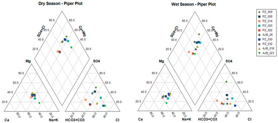
Figure 6.
Piper diagram for the ten wells sampled for groundwater quality in the dry and wet season. The legend refers to the ten groundwater sampling points assessed in this study and previously located in Figure 3.
As shown in Figure 7, Gibbs diagram confirms rock–water interaction processes to be most dominant in groundwater chemical composition, considering both dry and wet season results. A case in point is the presence of the bicarbonate anion. Its origin is related to the dissolution of carbonate in the geology of the study area, a process generated by the infiltration of rainwater and the slightly acidic conditions of the environment [57]. The presence of calcium is related to minerals such as calcite, dolomite, gypsum anhydrite, and fluorite, which are sources of this cation and are present in the sedimentary rocks of the studied formation. In addition, calcium is considered to be the most dominant alkaline earth metal [58].
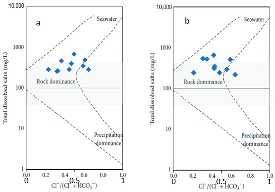
Figure 7.
(a) Gibbs diagram results during the dry season and (b) wet season.
Iron (Fe2+) and manganese (Mn+) have lower concentrations than the ions, but the values recorded are above those normally found in surface and underground waters, whose presence is evident in the samples collected, as they give a reddish color to the water. The presence of these minerals in groundwater is mainly due to the dissolution of rocks and minerals such as siderite, which are found in the ferrous state (Fe2+); given the anoxic conditions of the aquifer environment, once in contact with the atmosphere it oxidizes, changing to the ferric state (Fe3+), obtaining the appearance described above [53,59,60]. The identification of the exact minerals contributing to the presence of iron in the Arroyo Grande aquifer recures further mineralogic studies.
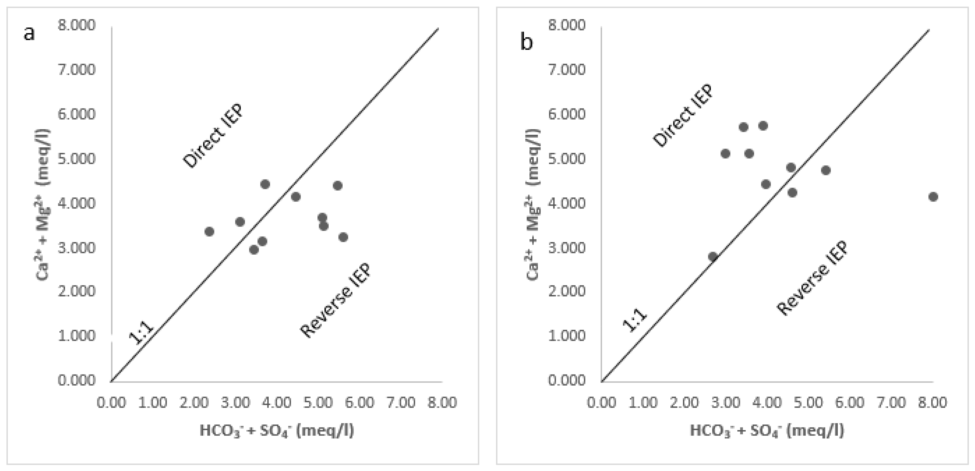
The ionic relationship graph Ca2+ + Mg2+ versus HCO3− + SO42−, prepared with data from the dry season (Figure 8a), shows that in addition to the mineral dissolution process already mentioned, reverse ion exchange processes (IEPs) are present, in which Ca2+ + Mg2+ are released into groundwater and Na+ and K+ are fixed to the aquifer material, causing water hardening [49]. The graphical data of the wet season (Figure 8b) show that the direct ion exchange process (IEP) together with mineralization are the most relevant processes during the wet season. This was also evidenced by the increase in sodium concentrations in the Arroyo Grande in the same season. The occurrence of IEP was also verified with the application of chloro-alkali indices (CAI).
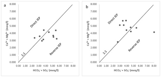
Figure 8.
(a) Ionic ratio Ca2+ + Mg2+ vs. HCO3− + SO42− results of sampling campaign No. 1—dry season; (b) ionic ratio Ca2+ + Mg2+ vs. HCO3− + SO42− results of sampling campaign No. 2 wet season.
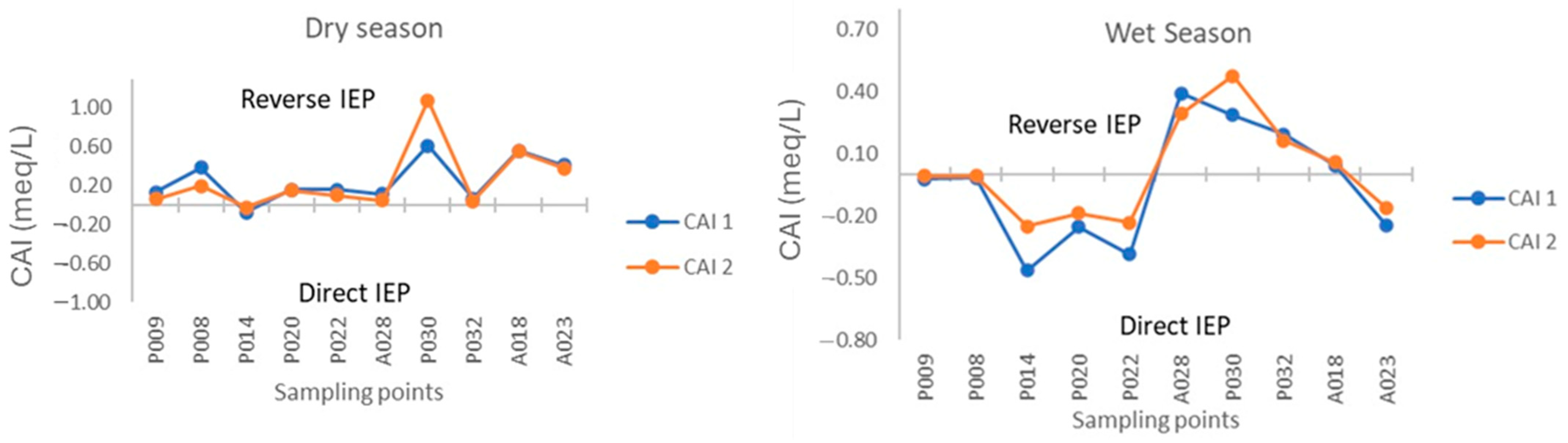
Figure 9 shows that the index values are mostly higher than zero for the data obtained from the first sampling campaign, confirming the occurrence of reverse ion exchange processes in the dry season. This changes for the data of the wet season, where the points of the graph show a tendency towards zero, indicating the occurrence of the direct IEP.
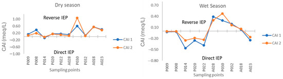
Figure 9.
Occurrence of direct or reverse ion exchange processes (IEPs) from the dry and wet season for both chloro-alkaline indices CAI 1 and CAI 2, as previously described in Equations (2) and (3).
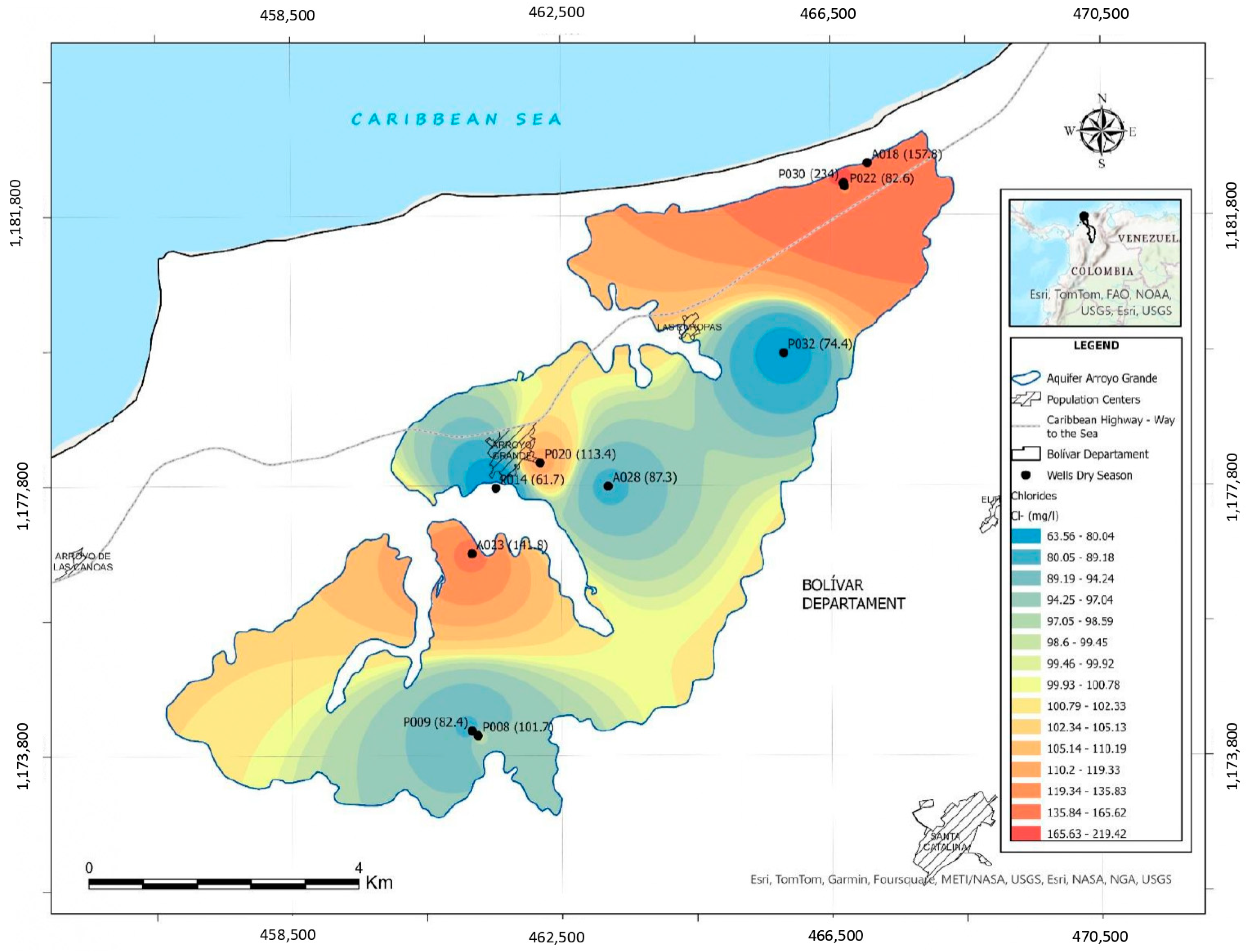
Salinization is another process evidenced by the chemical composition of the sampled water. This can occur in onshore areas due to the dumping of untreated wastewater or due to the intrusion of seawater. Due to their hydraulic connection with the sea, coastal aquifers are subject to the intrusion of seawater with a high salinity content, a process that occurs with the rupture of the equilibrium or transition zone, generated by the increase in sea levels and the overexploitation of the aquifer [61]. From the Cl anion, it was possible to analyze the changes to which the groundwater is exposed due to salinization processes.
The sampling point PZ N°030, which corresponds to a deep well (80 m) located 680 m from the coast, showed Cl− concentrations of 234 mg/L in the dry season and 226.9 mg/L in the wet season. In the case of water with neutral and natural pH, the expected concentration range of this anion is from 1.8 to 71 mg/L [42]. Therefore, an increase in chloride concentrations can be detected, which decreases inland from the coast as shown in the isoline map of Figure 10, except for sampling point AJ N°023, which corresponds to a cistern. Point AJ N°023 draws water from the shallow aquifer and shows higher chloride concentrations than the deep wells in the sector due to the infiltration of wastewater from septic systems.

Figure 10.
Isoline map of chloride in groundwater—dry season. The concentration of each sampling point is presented in parentheses.
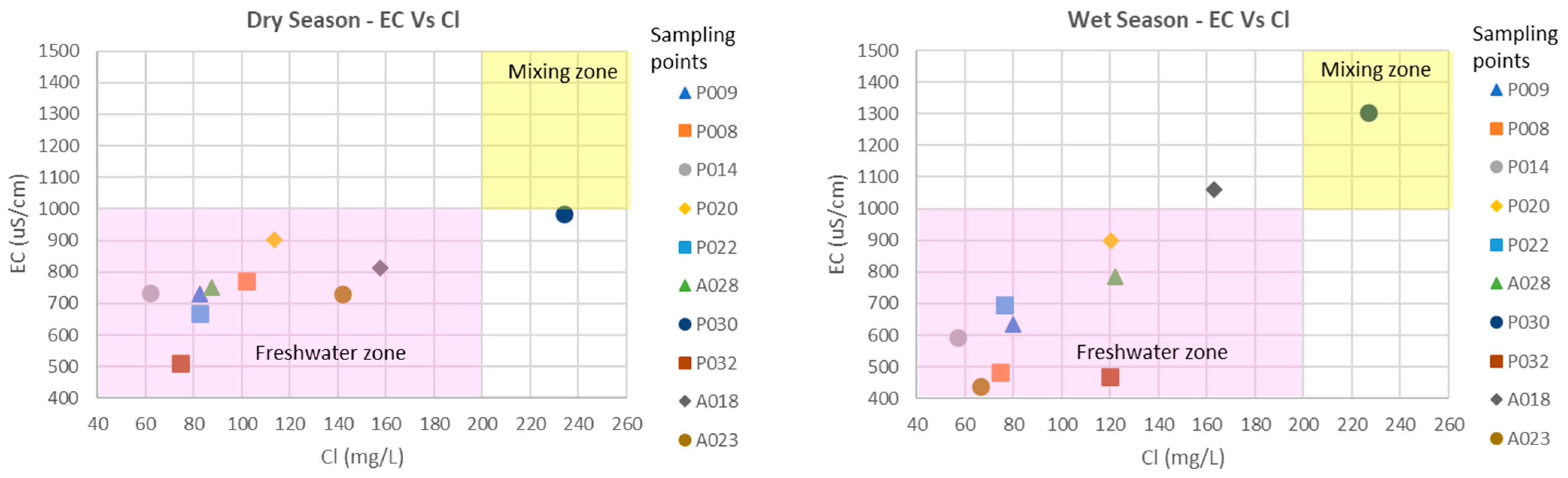
Similarly, the dispersion graph (Figure 11), constructed from the parameters of electrical conductivity (EC) and chlorides (Cl−), depicts that the wells near the coast are located in an area of mixing of fresh water with seawater. Near the coast, Cl− exceed concentrations of 200 mg/L and EC greater than 1000 mS/cm [24], occurring both in dry and wet seasons.
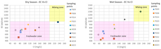
Figure 11.
Relationship between EC and Cl− for dry and wet season—the purple zone depicts the freshwater zone (groundwater samples with Cl− concentration less than 200 mg/L and EC~1000 µS/cm) and the yellow zone represent the mixing zone between fresh water and seawater (groundwater samples with Cl− exceeding 200 mg/L and EC exceeding 1000 µS/cm).
4.2. Principal Component Analysis (PCA)
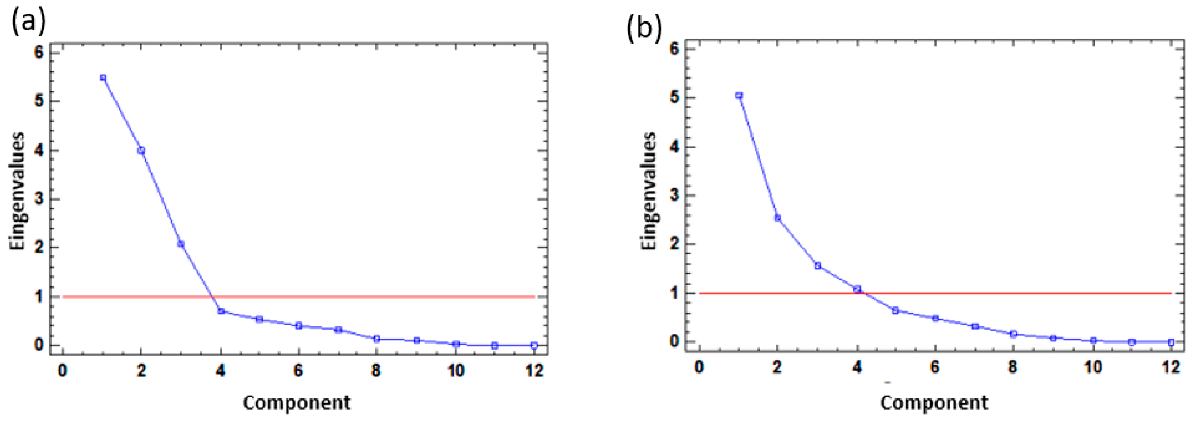
For the multivariate analysis, a total of 12 parameters were considered in 14 sampling points, pH, CE, TDS, Cl−, HCO3−, NO3−, SO42−, Fe2+, Na+, Ca2+, Mg2+, and Mn+. The application of the principal component analysis to the standardized data of sampling campaign No. 1 shows that three components explain 83.5% of the total variance of this group of data, with three components obtaining eigenvalues greater than or equal to one, a condition that can be observed in the sedimentation plot of Figure 12a.
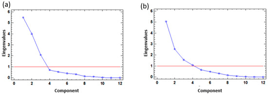
Figure 12.
(a) Sedimentation graph PCA analysis data sampling from the dry season and (b) the wet season.
In the case of the data from the second sampling campaign, the sedimentation graph suggests taking four components, but considering the variance provided by each of them, the first three are the most representative and provide an accumulated variance of 76.36% (Figure 12b).
The first component of the dry season explains 39.61% of the variance (Table 8), where the variables EC, TDS, HCO3−, Ca2+, and Mg2+ are the ones with the greatest loadings, indicating mineral dissolution processes such as calcite and dolomite [25,49].
Table 8.
Principal component loadings. In bold are highlighted the variables with the highest loading for each component.
The variables with the greatest loadings in component two are Na+ and NO3−, with 28.85% of the total variance, which owe their presence in the chemical composition of the water to ion exchange processes in the case of sodium and anthropogenic contamination. Chloride (Cl−) is the variable with the greatest loadings in component three, which explains 15.03% of the total variance. This anion is mainly related to salinization processes, either by seawater intrusion or by liquid waste dumping [55,62].
The PCA results for the wet season show that the first component explains 42.07% of the total variance. The variables with the largest loadings were CE, TDS, Cl−, and Na+ and to a lesser extent Ca2+ and Mg2+. It can be noted that the direct ion exchange process, with a contribution of sodium to the composition of the water, is the factor that determines this component, along with salinization processes. Component two accounts for 21.27% of the total variance for this data group, with Fe2+, Mn+, Ca2+, and Mg2+ as the variables with the greatest weight. In addition to mineral dissolution processes, the increase in iron and manganese concentrations can be related to sulfate and nitrate reduction processes [56].
Finally, component three has a variance of 21.27% of the total variance; the variables with the greatest loadings are HCO3−, NO3−, and Ca2+, related to mineral dissolution processes and anthropogenic activity.
In both the dry season and wet seasons, mineral dissolution processes and ion exchange processes influence the water quality, with the latter becoming more relevant during the wet season. This is evidenced by the types of water obtained according to the data of the second sampling campaign, where sodium (Na+) becomes one of the predominant cations in groundwater and the variable with the greatest weight in component number one for this group of data.
4.3. Water Quality Index (WQI)
The results obtained through the application of the WQI show that the water in the study area is not suitable for drinking purposes according to the water quality standards. For the two sampling campaigns, more than 50% of the surface and groundwater points were found to be unsuitable for drinking according to the classification based on the WQI value (Table 9). Less than 30% of the sampling points have a good water quality status. In the specific case of groundwater, which shows the most unfavorable quality conditions, the concentrations of iron and manganese impacted the calculation of the WQI. Other elements, such as calcium, magnesium, sodium, and bicarbonates, which are introduced into the water through mineral dissolution processes, increase the mineralization state of the groundwater and affect the quality of the water [63]. Regarding the high presence of iron and manganese in groundwater, it should be noted that prolonged consumption of high concentrations of these minerals can cause diseases such as Alzheimer’s, Huntington’s, Parkinson’s, and other cardiovascular and respiratory diseases, as well as cognitive impairments [53].
Table 9.
Classification of water samples according to water quality status.
5. Conclusions
The proposed framework offered a systematic and robust approach to groundwater quality assessment, addressing key challenges in understanding and managing complex hydrochemical systems. By integrating advanced analytical tools and data-driven methodologies, this framework contributes to advancing scientific knowledge and informs evidence-based decision-making for sustainable water resource management. Some of the key findings of the application of the framework in the Arroyo Grande aquifer include the following:
- The groundwater and surface waters of the aquifer evidenced distinct levels of mineralization due to the occurrence of mechanisms such as mineral dissolution, ion exchange, seawater intrusion, and anthropogenic contamination.
- The characteristics acquired by the water affected the availability of freshwater suitable for drinking for the communities near the area, to the point that in the dry and wet seasons, at least 50% of the sampled groundwater points are inadequate for drinking and fish farming.
- The groundwater of the Arroyo Grande hydrogeological unit exhibits high spatial and temporal variability in its main components. The heterogeneity and dynamics of this aquifer are evidenced in the several types of water found, which correspond to sodium sulfate, calcium bicarbonate, sodium chloride, sodium bicarbonate, magnesium sulfate, and magnesium chloride.
- The dominant elements in the Arroyo Grande water chemistry are the anions bicarbonate, chloride, and sulfate, in addition to cations sodium, calcium, and magnesium. The rock–water interaction mechanism is the most relevant in defining the chemical signature of the groundwater, through mineral dissolution and ion exchange processes related to the geological information of the area. The identification of the exact minerals that are contributing to the presence of Fe in the groundwater of the Arroyo Grande aquifer requires further mineralogical studies.
- Other factors affecting the chemical composition are the intrusion of seawater and anthropogenic activities. An increase in the saline intrusion phenomenon has been observed, currently affecting the extraction points near the coastal strip, which have high values of electrical conductivity and chlorides. Concentrations of iron and manganese are higher than drinking water standards, which requires constant monitoring of these parameters.
It is necessary to establish a monitoring network that allows the timely and adequate monitoring of the dynamics of the system. This is key to the development of mitigation strategies to improve the quality of the resource and strengthen its resilience against anthropogenic and climate change dynamics that threaten the sustainability of groundwater in the Arroyo Grande region.
Supplementary Materials
The following supporting information can be downloaded at: https://www.mdpi.com/article/10.3390/w16121650/s1, Supplementary Material S1.
Author Contributions
Conceptualization, C.A.-F., D.C.C., G.G.-R. and E.Q.-B.; Formal analysis, C.A.-F., D.C.C., G.G.-R. and E.Q.-B.; Resources, G.G.-R. and E.Q.-B.; Data curation, C.A.-F. and D.C.C.; Writing—original draft, C.A.-F.; Writing—review & editing, D.C.C. and E.Q.-B.; Supervision, D.C.C., G.G.-R. and E.Q.-B.; Project administration, E.Q.-B.; Funding acquisition, D.C.C. and E.Q.-B. All authors have read and agreed to the published version of the manuscript.
Funding
This work was financed by Minciencias (Ministry of science, technology, and innovation), OCAD and the fund for science, technology, and innovation of General royalties’ system in Colombia (FCTel-SGR) through the Convocatoria 8 and project BPIN 2020000100372, and the financial support of the Emerging Leaders of the Americas Program (ELAP). This research work was developed within the framework of the execution of the project “Hydrogeological and environmental profile of the Arroyo Grande coastal aquifer considering the effects of climate change and anthropogenic dynamics in the northern zone of the department of Bolívar” in cooperation between the University of Cartagena and the University of Sucre.
Data Availability Statement
Data are contained within the article and Supplementary Materials.
Conflicts of Interest
The authors declare no conflict of interest.
Appendix A
Table A1.
Summary of reviewed groundwater hydrochemical studies of costal aquifers.
Table A1.
Summary of reviewed groundwater hydrochemical studies of costal aquifers.
| System | Geology | Study Season | Types of Water Identified | Dominant Ions | Dominant Hydrochemical Processes a | Applied Hydrochemical Analysis b | Ref. | |
|---|---|---|---|---|---|---|---|---|
| Rock | Minerals | |||||||
| Morrosquillo Aquifer, Colombia | Sedimentary rock and sedimentary deposits | Calcite Dolomite Quartz Cast Halita | Dry and wet season | HCO3-Ca-Mg Cl-Na HCO3-Na | Dry season: Cation: Na+ > Ca2+ > Mg2+ > K+ Anion: HCO3− > Cl− > SO42− Wet season: Cation: Na+ > Ca2+ > Mg2+ > K+ Anion: HCO3− > Cl− > SO42− | R, I, S | PD, SP, SF | [6] |
| Recife metropolitan region aquifer, Brasil | Sedimentary rock | Calcite Dolomite Cast | Not indicated | Cl-Na HCO3-Na HCO3-Ca SO42-Ca | Cation: Na+ > Mg2+ > Ca2+ > K+ Anion: Cl− > HCO3− > SO42− > NO3− | R, I, W, P, A | G, IR, PD, ST, SF | [17] |
| Southwest Indian coastal aquifer, India | Igneous and metamorphic rocks (laterite, migmatite, granodiorite, and peninsular gneiss) | Quartz, feldspar, micas, muscovite, biotite, and amphibole | Pre-monsoon (may), monsoon, post (Sept) monsoon (January) | HCO3-Ca-Mg Cl-Ca Cl-SO42-Na Cl-SO42-Ca | Pre-monsoon Cation: Na+ > Ca2+ Anion: Cl− > HCO3− Monsoon Cation: Ca2+ > Na+ Anion: HCO3− > Cl− Post monsoon Cation: Ca2+ > Na+ Anion: HCO3− > Cl− | R, I | G, IR, PD, ST, CAI | [20] |
| Gaza coastal aquifer, Palestine | Sedimentary rock and sedimentary deposits | Calcite Dolomite Halite | Not indicated | Cl-Na HCO3-Na mixta Cl-Ca-Mg Ca/Mg–NO3/HCO3 | Cation: Ca2+ > Na+ > Mg2+ Anion: HCO3− > Cl− >SO42− | R, I, S, W, P | IR, PD, ST, CAI, CH, SP | [21] |
| Multilayered aquifers, Lower Kelantan Basin, Malaysia | Sedimentary rock and sedimentary deposits (shale, sandstone, phyllite, and slate) | Quartz Muscovite Sericite Dolomite Mica Goethite Hematite | Not indicated | HCO3-Ca HCO3-Na | Cation: Na+ > Ca2+ > Mg2+ > K+ Anion: HCO3− > Cl− > SO42− > CO3− | R, I, S, W, F | IR, PD, ST, SP | [22] |
| Lagos coastal belt aquifer, Nigeria | Sedimentary rock and sedimentary deposits | Calcite Dolomite Cast | Dry and wet season | Dry season: HCO3-Ca HCO3-Ca-Mg Wet season: HCO3-Ca-Mg Cl-SO42-Ca–Mg Cl-Ca-Mg Cl-Ca | Dry season: Cation: Ca2+ > K+ > Na+ > Mg2+ Anion: HCO3− > Cl− Wet season: Cation: Ca2+ > Mg2+ > K+ > Na+ Anion: Cl− > HCO3− > SO42− | R, I, S, M | IR, PD, SP, D, GM | [23] |
| Various mediterranean coast aquifers * | Sedimentary rock and sedimentary deposits | Calcite Dolomite Yeso anhydrite | Not indicated | Cl-Na Cl-ca HCO3-Ca HCO3-Na SO42-Ca-Mg | Cation: Na+ > Ca2+ > Mg2+ Anion: Cl− > SO42− > HCO3− | R, I, S, A | IR, PD, ST, SI | [24] |
| Quintana Roo southern zone aquifer, Mexico | Sedimentary rocks (Limestone-dolimias-evapotites) | Dolomite Aragonite Cast Halite | Wet season | HCO3-Ca Cl-Ca-Mg SO42-Ca Cl-Na | Cation: Ca2+ > Na+ > Mg2+ > K+ Anion: HCO3− > SO42− > Cl− > NO3− | R, I, S, A | PD, ST | [25] |
| Arroyo Grande aquifer, Colombia | Sedimentary rock and sedimentary deposits | Calcite Dolomite Quartz Halita | Dry and wet season | HCO3-Ca HCO3-Na Cl-Na SO42-Na Cl-Mg SO42-Mg | Dry season: Cation: Na+ > Ca2+ > Mg2+ > Fe2+ Anion: HCO3− > Cl− > SO42− > NO3− Wet season: Cation: Na+ > Ca2+ > Mg2+ > Fe2+ Anion: HCO3− > Cl− > SO42− > NO3− | R, I, S, A | G, IR, PD, CAI, ST, SP | This study |
Notes: * The Plio-Quaternary aquifer of Jerba Island (Tunisia), the Upper Miocene–Pliocene–Quaternary aquifer of Tripoli (Libya), the Plio-Quaternary aquifer of Nador plain (Algeria), the Bou Areg Plio-Quaternary aquifer (Morocco), the Miocene carbonate aquifer of Porto Torres (NW Sardinia, Italy), and the Pleistocene oolitic aquifer of the Baghoush area (Egypt). a R (rock dissolution), I (ion exchange), S (seawater mixing), W (sewage infiltration), P (rainfall recharge), F (agrochemical fertilizers mixing), A (anthropogenic pollutants mixing), M (simple mixing and evaporation). b G (Gibbs plot), IR (ionic ratios), PD (Piper diagram), CAI (CAI plot), ST (statistics), CH (Chadha plot), SP (Schoeller plot), SI (seawater intrusion index statistics), D (Durov diagram), GM (geochemical modeling statistics), SF (Stiff plot).
Table A2.
Lithological column of SEV 10.
Table A2.
Lithological column of SEV 10.
| Layer | Lithology SEV 10 | Resistivity (Ω.m) | Thickness (m) | Depth (m) |
|---|---|---|---|---|
| 1 | Topsoil covered by sand and gravel | 540.9 | 3.4 | 3.4 |
| 2 | Dry granular material (sands and gravels) | 228.8 | 5.4 | 8.8 |
| 3 | Saturated granular material (sands and gravels) | 84.9 | 13.9 | 22.7 |
| 4 | Saturated fine granular materials (sands, gravels, clays, and silts) | 35.8 | 94.8 | 117.5 |
| 5 | Saturated granular material (sands and gravels) | 78.4 | - | - |
Table A3.
Lithological column of SEV 13.
Table A3.
Lithological column of SEV 13.
| Layer | Lithology SEV 13 | Resistivity (Ω.m) | Thickness (m) | Depth (m) |
|---|---|---|---|---|
| 1 | Vegetation covered by sand, gravel, and silt | 199.7 | 0.8 | 0.8 |
| 2 | Fine to dry granular materials (sands, clays, and silt) | 18.5 | 0.5 | 1.3 |
| 3 | Saturated granular material (sands) | 104.2 | 10.5 | 11.8 |
| 4 | Saturated granular material (sands and gravels) | 214.3 | 8.0 | 19.8 |
| 5 | Fine to saturated granular materials (few sands, clays, and silt) | 7.6 | 25.9 | 45.7 |
| 6 | Saturated granular materials (sands, gravels, and silt) | 56.9 | 85 | 130.7 |
| 7 | Fine to saturated granular materials (few sands, clays, and silt) | 8.8 | ? | ? |
Table A4.
Analytical errors from the laboratory analyses.
Table A4.
Analytical errors from the laboratory analyses.
| Parameter | Analysis | Uncertainty (±) |
|---|---|---|
| Anions | Nitrates | 0.033 |
| Anions | Fluorides | 0.039 |
| Anions | Nitrites | 0.033 |
| Anions | Sulphate | 0.071 |
| Principal ions or minerals | Total alkalinity | 0.05 |
| Principal ions or minerals | Sulphate | 0.04 |
| Principal ions or minerals | Carbonates | 0.057 |
| Principal ions or minerals | Bicarbonates | 0.057 |
| Nutrients | Nitrite | 0.001 |
| Nutrients | Total nitrogen Kjeldahl | 0.01 |
| Nutrients | Total phosphorus | 0.03 |
| Principal ions or minerals | Total calcium | 0.03 |
| Principal ions or minerals | Total magnesium | 0.13 |
| Principal ions or minerals | Total potassium | 0.04 |
| Principal ions or minerals | Total sodium | 0.05 |
| Trace metals | Total arsenic | 0.13 |
| Trace metals | Total boro | 0.03 |
| Trace metals | Total iron | 0.05 |
| Trace metals | Total manganese | 0.13 |
| Trace metals | Total mercury | 0.13 |
| Trace metals | Total lead | 0.14 |
| Trace metals | Total selenio | 0.16 |
References
- Post, V.; Eichholz, M.; Brentfuerher, R. Groundwater management in Coastal Zones; Bundesanstalt für Geowissenschaften und Rohstoffe (BGR): Hannover, Germany, 2018. [Google Scholar]
- Custodio, E. Trends in Groundwater Pollution: Loss of Groundwater Quality and Related Services; Groundwater Governance: Delft, The Netherlands, 2011. [Google Scholar]
- IDEAM—Instituto de Hidrología, Meteorología y Estudios Ambientales. Estudio Nacional del Agua; IDEAM: Bogota, Colombia, 2022. [Google Scholar]
- Chala, D.C.; Quiñones-Bolaños, E.; Mehrvar, M. An integrated framework to model salinity intrusion in coastal unconfined aquifers considering intrinsic vulnerability factors, driving forces, and land subsidence. J. Environ. Chem. Eng. 2022, 10, 106873. [Google Scholar] [CrossRef]
- UNESCO. UN-Water: United Nations World Water Development Report 2020: Water and Climate Change; UNESCO: Paris, France, 2020. [Google Scholar]
- Martinez, D.C.; Betancur, T.; Herrera, H.M. Hydrogeochemical assessment and modeling of Morrosquillo Coastal Aquifer (Sucre-Colombia). Rev. Fac. Ing. 2014, 71, 126–140. [Google Scholar] [CrossRef]
- Gomez Arevalo, E.D. A Groundwater Flow Model to Aid in Water Resource Management for the Carraipia Basin in the Coastal Semi-Arid Region of La Guajira State (Colombia); The University of Maine: Orono, ME, USA, 2020; p. 83. [Google Scholar]
- Cardique, Identificacion de la Vulnerabilidad del Acuifero Costero de Arroyo Grande Ante la Intrusion Salina; Cardique: Cartagena, Colombia, 2006.
- Restrepo-Ángel, J.D.; Mora-Páez, H.; Díaz, F.; Govorcin, M.; Wdowinski, S.; Giraldo-Londoño, L.; Tosic, M.; Fernández, I.; Paniagua-Arroyave, J.F.; Duque-Trujillo, J.F. Coastal subsidence increases vulnerability to sea level rise over twenty first century in Cartagena, Caribbean Colombia. Sci. Rep. 2021, 11, 18873. [Google Scholar] [CrossRef]
- Hincapie, G.; Hueguett, A. Memoria Tecnica de la Plancha 5-04-Atlas de Aguas Subterraneas de Colombia pdf; Bogotá, Colombia, 2003. Available online: https://recordcenter.sgc.gov.co/B3/12006050020005/documento/Pdf/29.MemoriaPL5-04.pdf (accessed on 10 July 2022).
- CARDIQUE. Hidrogeologos Estudio Hidrogeologico del Acuifero de Arroyo Grande; CARDIQUE: Bolivar, Colombia, 1999. [Google Scholar]
- Chala, D.C.; Jiménez, T.; Rodríguez, D.; Quinoñes, E.; Mehrvar, M.; St, V.; Mb, O.N.; Carolina, D.; Diaz, C.; Bolaños, E.Q. Groundwater governance of coastal aquifers in the Colombian Caribbean Region, South America: Call to action to strengthen aquifers resilience and groundwater use against climate change effects. In Proceedings of the International Young Water Professionals Conference, Toronto, ON, Canada, 23 June 2019. [Google Scholar]
- Machiwal, D.; Jha, M.K. Identifying sources of groundwater contamination in a hard-rock aquifer system using multivariate statistical analyses and GIS-based geostatistical modeling techniques. J. Hydrol. Reg. Stud. 2015, 4, 80–110. [Google Scholar] [CrossRef]
- Aldhyani, T.H.H.; Al-Yaari, M.; Alkahtani, H.; Maashi, M. Water Quality Prediction Using Artificial Intelligence Algorithms. Appl. Bionics Biomech. 2020, 2020, 6659314. [Google Scholar] [CrossRef]
- Malik, A. Sugandh Groundwater hydro-geochemistry, irrigation and drinking quality, and source apportionment in the intensively cultivated area of Sutlej sub-basin of main Indus basin. Environ. Earth Sci. 2022, 81, 456. [Google Scholar] [CrossRef]
- Islam, A.R.M.T.; Kabir, M.M.; Faruk, S.; Al Jahin, J.; Bodrud-Doza, M.; Didar-ul-Alam, M.; Bahadur, N.M.; Mohinuzzaman, M.; Fatema, K.J.; Safiur Rahman, M.; et al. Sustainable groundwater quality in southeast coastal Bangladesh: Co-dispersions, sources, and probabilistic health risk assessment. Environ. Dev. Sustain. 2021, 23, 18394–18423. [Google Scholar] [CrossRef]
- Silva, T.R.; Leitão, T.E.; Lima, M.M.C.; Martins, T.N.; Oliveira, M.M.; Albuquerque, M.S.C.; Costa, W.D. Hydrogeochemistry and isotope compositions of multi-layered aquifer systems in the Recife Metropolitan Region, Pernambuco (NE Brazil): An integrated approach using multivariate statistical analyses. J. S. Am. Earth Sci. 2021, 109, 103323. [Google Scholar] [CrossRef]
- Pohl, C. From science to policy through transdisciplinary research. Environ. Sci. Policy 2008, 11, 46–53. [Google Scholar] [CrossRef]
- Pahl-Wostl, C.; Holtz, G.; Kastens, B.; Knieper, C. Analyzing complex water governance regimes: The Management and Transition Framework. Environ. Sci. Policy 2010, 13, 571–581. [Google Scholar] [CrossRef]
- Akshitha, V.; Balakrishna, K.; Udayashankar, H.N. Assessment of hydrogeochemical characteristics and saltwater intrusion in selected coastal aquifers of southwestern India. Mar. Pollut. Bull. 2021, 173, 112989. [Google Scholar] [CrossRef]
- Alnaeem, M.A.; Yusoff, I.; Ng, T.; Alias, Y.; May, R.; Haniffa, M. An integrated multi-techniques approach for hydrogeochemical evaluation of ion exchange processes and identification of water types based on statistical analysis: Application to the Gaza coastal aquifer, Gaza Strip, Palestine. Groundw. Sustain. Dev. 2019, 9, 100227. [Google Scholar] [CrossRef]
- Sefie, A.; Aris, A.Z.; Ramli, M.F.; Narany, T.S.; Shamsuddin, M.K.N.; Saadudin, S.B.; Zali, M.A. Hydrogeochemistry and groundwater quality assessment of the multilayered aquifer in Lower Kelantan Basin, Kelantan, Malaysia. Environ. Earth Sci. 2018, 77, 397. [Google Scholar] [CrossRef]
- Yusuf, M.A.; Abiye, T.A.; Ibrahim, K.O.; Abubakar, H.O. Hydrogeochemical and salinity appraisal of surficial lens of freshwater aquifer along Lagos coastal belt, South West, Nigeria. Heliyon 2021, 7, e08231. [Google Scholar] [CrossRef] [PubMed]
- Telahigue, F.; Mejri, H.; Mansouri, B.; Souid, F.; Agoubi, B.; Chahlaoui, A.; Kharroubi, A. Assessing seawater intrusion in arid and semi-arid Mediterranean coastal aquifers using geochemical approaches. Phys. Chem. Earth 2020, 115, 102811. [Google Scholar] [CrossRef]
- Sánchez-Sánchez, J.A.; Álvarez-Legorreta, T.; Pacheco-Ávila, J.G.; González-Herrera, R.A.; Carrillo-Bribiezca, L. Caracterización hidrogeoquímica de las aguas subterráneas del sur del Estado de Quintana Roo, México. Rev. Mex. Ciencias Geol. 2015, 32, 62–76. [Google Scholar]
- Cao, T.; Han, D.; Song, X. Past, present, and future of global seawater intrusion research: A bibliometric analysis. J. Hydrol. 2021, 603, 126844. [Google Scholar] [CrossRef]
- Sánchez, J.A.; Álvarez, T.; Pacheco, J.G.; Carrillo, L.; González, R.A. Calidad del agua subterránea: Acuífero sur de Quintana Roo, México. Tecnol. Ciencias Agua 2016, 7, 75–96. [Google Scholar]
- Abascal, E.; Gómez-Coma, L.; Ortiz, I.; Ortiz, A. Global diagnosis of nitrate pollution in groundwater and review of removal technologies. Sci. Total Environ. 2022, 810, 152233. [Google Scholar] [CrossRef]
- IDEAM. Consulta y Descarga de Datos Hidrometeorológicos. 2023. Available online: http://dhime.ideam.gov.co/atencionciudadano (accessed on 27 July 2022).
- Briceño, A.M. Dinámica del Crecimiento y Relación con el Clima de Especies Arbóreas de los Bosques de la Región Caribe, Colombia. Ph.D. Thesis, Universidad Nacional de Colombia, Bogotá, DC, Colombia, 2017. [Google Scholar]
- Murtinho, F.; Tague, C.; de Bievre, B.; Eakin, H.; Lopez-Carr, D. Water Scarcity in the Andes: A Comparison of Local Perceptions and Observed Climate, Land Use and Socioeconomic Changes. Hum. Ecol. 2013, 41, 667–681. [Google Scholar] [CrossRef]
- IDEAM. Estudio Nacional del Agua 2014; IDEAM: Bogota, Colombia, 2015. [Google Scholar]
- Guzmán, G.; Gómez, E.; Serrano, B. Geología de los Cinturones Del Sinú, San Jacinto y Borde Occidental del Valle Inferior del Magdalena Caribe Colombiano; Servicio Geológico Colombiano: Bogota, Colombia, 2004. [Google Scholar]
- Reyes, G.; Guzmán, O.; Gonzalo, B.; Zapata, G. Geología de las Planchas 23 Cartagena y 29–30 Arjona-Memoria Explicativa; Bogotá D.C. 2001. Available online: https://www2.sgc.gov.co/MGC/Documents/MGC_2023/Memoria_mgc_gmc_agc_2023.pdf (accessed on 26 July 2022).
- Gomez, J.; Montes, N.E.; Marín, E. Mapa Geologico de Colombia 2023 Escala 1:1 500 000; Servicio Geológico Colombiano: Bogota, Colombia, 2023. [Google Scholar]
- Alcaldia de Cartagena de Indias. Consultorias y Servicios Juridicos y Comerciales Consultoría para la Elaboración de los Estudios, Análisis y Mediciones Necesarios para la Administración, Adquisición y Mantenimiento de Predios que Integran las Áreas de Interés Estratégico que Surten al Acueducto de Cartagena, Contrato no. c. 2018; Alcaldia de Cartagena de Indias: Bolívar, Colombia, 2018. [Google Scholar]
- Waterloo Hydrogeologic. AquaChem 11.0 Student License, Canada. Computacional Program 2022. Canada, 2022. Available online: http://www.waterloohydrogeologic.com/AquaChem (accessed on 27 July 2022).
- Leite, C.M.; Wendland, E.; Gastmans, D. Caracterização hidrogeoquímica de águas subterrâneas utilizadas para abastecimento público na porção nordeste do Sistema Aquífero Guarani. Eng. Sanit. Ambient. 2021, 26, 29–43. [Google Scholar] [CrossRef]
- APHA; AWWA; WEF. Standard Methods for the Examination of Water and Wastewater, 23rd ed.; American Public Health Association: Whashington, DC, USA, 2017. [Google Scholar]
- NTC-ISO 5667-1; Enviromental Management Water Quality Sampling Huidance on the Desing of Sampling Programmes. ICONTEC: Bogotá, Colombia, 1995.
- Pfaff, J.D. Determination of Inorganic Anions By Ion Chromatography. Methods Determ. Met. Environ. Samples 1996, 388–417. [Google Scholar] [CrossRef]
- USEPA. USEPA Method 200.8. US Environ. Prot. Agency 1994, 4, 1–57. [Google Scholar]
- IDEAM. Principios Básicos para el Conocimiento y Monitoreo de las AGUAS subterráneas-Contenidos del Taller de Formación; IDEAM: Bogota, Colombia, 2015. [Google Scholar]
- University of Amsterdam. JASP 9.2 Free Software, Amsterdan. Computacional Program 2018. Available online: https://jasp-stats.org/ (accessed on 27 July 2022).
- Gopal, V.; Achyuthan, H.; Jayaprakash, M. Hydrogeochemical characterization of Yercaud lake southern India: Implications on lake water chemistry through multivariate statistics. Acta Ecol. Sin. 2018, 38, 200–209. [Google Scholar] [CrossRef]
- Omonona, O.V.; Okogbue, C.O. Geochemistry of rare earth elements in groundwater from different aquifers in the Gboko area, central Benue Trough, Nigeria. Environ. Earth Sci. 2017, 76, 8. [Google Scholar] [CrossRef]
- Heikhy Narany, T.; Sefie, A.; Aris, A.Z. The long-term impacts of anthropogenic and natural processes on groundwater deterioration in a multilayered aquifer. Sci. Total Environ. 2018, 630, 931–942. [Google Scholar] [CrossRef] [PubMed]
- Cloutier, V.; Lefebvre, R.; Therrien, R.; Savard, M.M. Multivariate statistical analysis of geochemical data as indicative of the hydrogeochemical evolution of groundwater in a sedimentary rock aquifer system. J. Hydrol. 2008, 353, 294–313. [Google Scholar] [CrossRef]
- Zakaria, N.; Anornu, G.; Adomako, D.; Owusu-nimo, F.; Gibrilla, A. Evolution of groundwater hydrogeochemistry and assessment of groundwater quality in the Anayari catchment. Groundw. Sustain. Dev. 2020, 12, 100489. [Google Scholar] [CrossRef]
- Ghosh, A.; Bera, B. Hydrogeochemical assessment of groundwater quality for drinking and irrigation applying groundwater quality index (GWQI) and irrigation water quality index (IWQI). Groundw. Sustain. Dev. 2023, 22, 100958. [Google Scholar] [CrossRef]
- Varol, S.; Davraz, A. Evaluation of the groundwater quality with WQI (Water Quality Index) and multivariate analysis: A case study of the Tefenni plain (Burdur/Turkey). Environ. Earth Sci. 2015, 73, 1725–1744. [Google Scholar] [CrossRef]
- Kouassy Kalédjé, P.S.; Mfonka, Z.; Ntsama, I.S.B.; Kpoumié, A.; Fouépé Takounjou, A.; Ndam Ngoupayou, J.R. Groundwater quality assessment in the catchment area of Kadey (East-Cameroon): Water quality index approach. Sustain. Water Resour. Manag. 2023, 9, 137. [Google Scholar] [CrossRef]
- Rushdi, M.I.; Basak, R.; Das, P.; Ahamed, T.; Bhattacharjee, S. Assessing the health risks associated with elevated manganese and iron in groundwater in Sreemangal and Moulvibazar Sadar, Bangladesh. J. Hazard. Mater. Adv. 2023, 10, 100287. [Google Scholar] [CrossRef]
- World Health Organization. Guidelines for Drinking-Water Quality: Fourth Edition Incorporating the First Addendum; SWISS: Geneva, Switzerland, 2017. [Google Scholar]
- Sunkari, E.D.; Seidu, J.; Ewusi, A. Hydrogeochemical evolution and assessment of groundwater quality in the Togo and Dahomeyan aquifers, Greater Accra Region, Ghana. Environ. Res. 2022, 208, 112679. [Google Scholar] [CrossRef] [PubMed]
- Malagon, J.P. Análisis Hidrogeoquímico Multivariado del Agua Subterránea del Sistema Acuífero del Valle Medio del Magdalena–Colombia. Ph.D. Thesis, Universidad Nacional de Colombia, Medellin, Colombia, 2017. [Google Scholar]
- Abu-alnaeem, M.F.; Yusoff, I.; Ng, T.F.; Alias, Y.; Raksmey, M. Assessment of groundwater salinity and quality in Gaza coastal aquifer, Gaza Strip, Palestine: An integrated statistical, geostatistical and hydrogeochemical approaches study. Sci. Total Environ. 2018, 615, 972–989. [Google Scholar] [CrossRef] [PubMed]
- Abdelshafy, M.; Saber, M.; Abdelhaleem, A.; Abdelrazek, S.M.; Seleem, E.M. Hydrogeochemical processes and evaluation of groundwater aquifer at Sohag city, Egypt. Sci. Afr. 2019, 6, e00196. [Google Scholar] [CrossRef]
- Guillen-rivas, J.R.; Jaramillo-Cedeño, A.R.; Baquerizo-Crespo, R.J.; Córdova-Mosquera, R.A. Estudio de los procesos de remoción de hierro y manganeso en aguas subterráneas: Una revisión. Polo Conoc. 2021, 6, 1384–1407. [Google Scholar]
- Usman, U.A.; Yusoff, I.; Raoov, M.; Hodgkinson, J. Trace metals geochemistry for health assessment coupled with adsorption remediation method for the groundwater of Lorong Serai 4, Hulu Langat, west coast of Peninsular Malaysia. Environ. Geochem. Health 2020, 42, 3079–3099. [Google Scholar] [CrossRef] [PubMed]
- Hounsinou, S.P. Assessment of potential seawater intrusion in a coastal aquifer system at Abomey-Calavi, Benin. Heliyon 2020, 6, e03173. [Google Scholar] [CrossRef] [PubMed]
- Balasubramanian, M.; Sridhar, S.G.D.; Ayyamperumal, R.; Karuppannan, S.; Gopalakrishnan, G.; Chakraborty, M.; Huang, X. Isotopic signatures, hydrochemical and multivariate statistical analysis of seawater intrusion in the coastal aquifers of Chennai and Tiruvallur District, Tamil Nadu, India. Mar. Pollut. Bull. 2022, 174, 113232. [Google Scholar] [CrossRef]
- Chaurasia, A.K.; Pandey, H.K.; Tiwari, S.K.; Pandey, P.; Ram, A. Groundwater vulnerability assessment using water quality index (WQI) under geographic information system (GIS) framework in parts of Uttar Pradesh, India. Sustain. Water Resour. Manag. 2021, 7, 40. [Google Scholar] [CrossRef]

Disclaimer/Publisher’s Note: The statements, opinions and data contained in all publications are solely those of the individual author(s) and contributor(s) and not of MDPI and/or the editor(s). MDPI and/or the editor(s) disclaim responsibility for any injury to people or property resulting from any ideas, methods, instructions or products referred to in the content. |
© 2024 by the authors. Licensee MDPI, Basel, Switzerland. This article is an open access article distributed under the terms and conditions of the Creative Commons Attribution (CC BY) license (https://creativecommons.org/licenses/by/4.0/).