Abstract
The Columbia River Basin faces a threat from the potential invasion of zebra mussels (Dreissena polymorpha), notorious for their ability to attach to various substrates, including concrete, which is common in fishway construction. Extensive mussel colonization within fishways may affect fish passage by altering flow patterns or creating physical barriers, leading to increased travel times, or potentially preventing passage altogether. Many factors affect mussel habitat suitability including vectors of dispersal, water parameters, and various hydrodynamic quantities, such as water depth, velocity, and turbulence. The objective of this study is to assess the potential for zebra mussels to attach to fishway surfaces and form colonies in the McNary Lock and Dam Oregon-shore fishway and evaluate the potential impact of this infestation on the fishway’s efficiency. A computational fluid dynamics (CFD) model of the McNary Oregon-shore fishway was developed using the open-source code OpenFOAM, with the two-phase solver interFoam. Mesh quality is critical to obtain a reliable solution, so the numerical mesh was refined near the free surface and all solid surfaces to properly capture the complex flow patterns and free surface location. The simulation results for the 6-year average flow rate showed good agreement with the measured water column depth over each weir. Regions susceptible to mussel infestation were identified, and an analysis was performed to determine the mussel’s preference to colonize as a function of the depth-averaged velocity, water depth, and wall shear stress. Habitat suitability criteria were applied to the output of the hydraulic variables from the CFD solution and provided insight into the potential impact on the fishway efficiency. Details on the mesh construction, model setup, and numerical results are presented and discussed.
1. Introduction
Zebra mussels (Dreissena polymorpha) have become a nuisance in North American waterways impacting structural and ecological systems, and costing hundreds of millions of dollars in structural and electrical damage due to biofouling [1,2,3,4]. Adult Dreissena possess high fecundity and can attach to submerged concrete substrates using their byssal threads, forming colonies up to 0.3 m thick. These colonies severely impede waterway flow and disturb existing hydraulic flow patterns, presenting a unique biological challenge [2,3,4,5]. There are concerns that large colonies may even deteriorate concrete substrates due to high ammonia levels [6]. Many dams have concrete fishways that are potentially susceptible to invasion but, to our knowledge, the impacts of mussel infestation on fishway operations have not been studied.
In the Columbia River, fishways are a primary management tool for mitigating hydropower development. Concerns about invasive mussel establishment in fishways arise from the extensive reliance on these structures. For example, salmonid fish passage may become delayed or impossible in extreme cases, if a large enough colony were to become established. The physical removal of colonized mussels would require dewatering and could be necessary annually or even more frequently depending on the growth rate, resulting in higher costs for the operation and maintenance of fishways [4]. Yearly fish passage reports from the United States Army Corps of Engineers (USACE) Northwestern Division report the detection of invasive species at USACE dams on the Columbia River and, as of 2022, no detections of Dreissena have been reported [7]. Although Dreissena have not yet been identified in the Columbia River Basin, biological models predict that potential zebra mussel invasion may vary in the mid- to upper Columbia River, with some regions meeting the criteria for being high risk [8,9,10]. Therefore, there is growing interest in assessing likely mussel settling locations if such an invasion was to occur.
Many factors may influence the extent of a potential invasion including vectors of dispersal, limnology, food availability, existing breeding population, and hydraulics [11]. It is well understood that the primary vessel for the transportation and settling of Dreissena is boat activity, posing a potential risk for portions of the lower Columbia River [11,12]. Predictive models have been developed to assess risk based on limnological parameters [2,13,14], and water parameters on the Columbia River have been noted to be favorable for colonization [4,9]. Hydraulics must also be considered due to the complex life history of Dreissena. Larval Dreissena (i.e., veliger) differ from their adult counterparts in that they are free swimming and thrive in planktonic and benthic regions, and laboratory experiments suggest that there are strong ties between veliger mortality and strong, turbulent hydrodynamic forces [3,15]. Some have attempted, through experimentation, to derive a more direct relationship between larval mortality and the Kolmogorov length scale as a function of the veliger shell size [16]. Others have studied the effect of various hydrodynamic variables, such as the velocity, depth, velocity to depth ratio, Froude number (Fr) shear stress, and Reynolds shear stress (RSS) on the presence of adult Dreissena and found that the most important factors in determining Dreissena’s colonization were a combination of velocity and water depth [17].
As computational resources become more advanced and efficient, two-phase computational fluid dynamics (CFD) modelling has become less expensive and more prevalent. OpenFOAM is an open-source CFD software package known for its efficiency and versatility, especially in modelling two-phase flows on complex geometries, and has even been found to rival the accuracy of commercial software packages in fishway analyses [18,19,20,21]. In this study, OpenFOAM’s built-in two-phase flow solver interFoam is utilized. A thorough summary of interFoam’s numerical methods and capabilities can be found in [22].
The purpose of the following analysis is to quantify the risk of invasive mussel colonization in the McNary Lock and Dam Oregon-shore fishway and to identify mussel settling locations. Numerical simulation conditions were conducted for a typical pool and tailwater elevation with a fixed flow rate, and gravity-fed diffusers provided additional attraction flow near the downstream end of the ladder. The model was validated using measured water depth over each weir in the fishway. This analysis seeks to provide a validated computational methodology to aid in understanding invasive species and their impact on fish passage through a fishway.
2. Study Area
The McNary Lock and Dam is a USACE hydroelectric facility that sits at river mile 292 on the Columbia River near Umatilla, Oregon, and is vital for the passage of lamprey and several species of salmon, including chinook, steelhead, sockeye, and coho [23]. McNary fish bypass systems consist of two adult fishways on the Washington (north) and Oregon (south) sides of the river, respectively. The Oregon shore fishway is 9.15 m wide, over 600 m long, and contains a regulating weir, seven tilting weirs, and eighty-five Ice Harbor-type weirs that are equally spaced at 6.1 m apart and span nearly the entire length of the fishway. The regulating and tilting weir positions are controlled via a computer program and are responsible for maintaining set discharge targets within the fishway. Flow enters the fishway from the forebay and travels approximately 80 m through the flat upper-most section of the fishway, before sloping downward (1:20 slope) for approximately 100 m. The fishway then turns at 90° from the flow direction and slopes downward for the following 40 m. Finally, the fishway turns 15° from the flow direction and slopes downward for the remaining 400 m, where the flow exits into the tailrace. A detailed model of the Oregon-shore fishway geometry was provided by USACE Walla Walla District, which was prepared for the numerical model by simplifying the fishway channel. Figure 1 shows the location of the Oregon-shore fishway model relative to the McNary spillway, forebay, and tailrace, with the vertical datum referenced to the mean sea level (MSL) in meters and contains detailed schematics of the fishway channel regarding its profile.
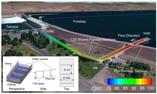
Figure 1.
A three-dimensional schematic shows the flat and sloped sections of the Oregon-shore fishway relative to the forebay and tailrace [24]. The zoomed-in section shows a perspective, side, and top view of the sloped sections of the fishway channel. The fishway weirs and bed are colored by the elevation in meters.
3. McNary Fishway Model
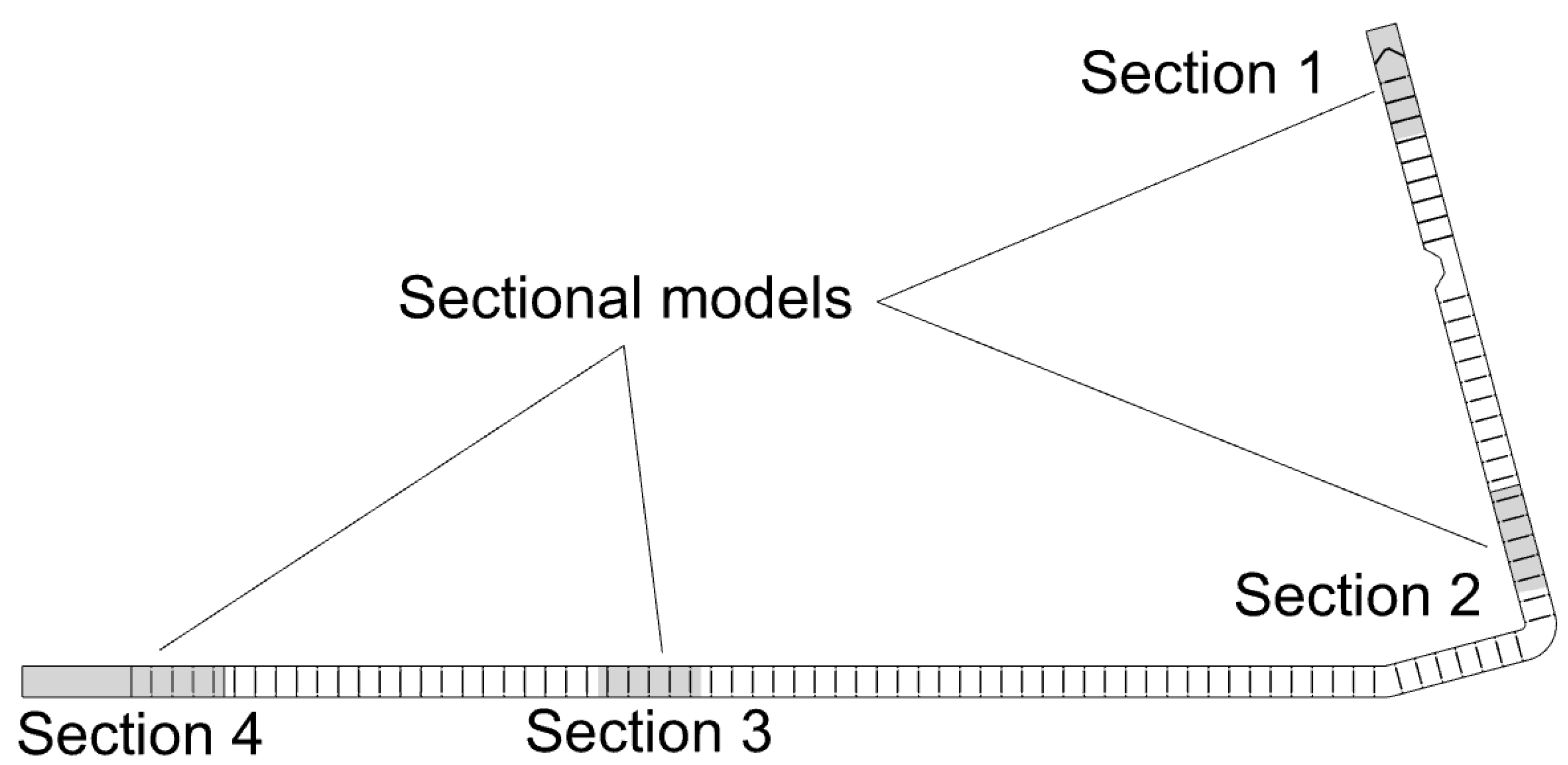
Five simulations were performed in the following analysis. Sim1 considers the entire Oregon-shore fishway, whereas Sim2–Sim5 are reduced sections of the fishway. The sectional models allow much finer control of the quality of the numerical mesh and faster convergence of the solution. The purpose of Sim1 was to determine the hydrodynamic flow patterns of the fishway to perform habitat suitability analysis based on water depth and depth-averaged velocity and to provide the boundary conditions for the sectional models. The purpose of Sim2–Sim5 was to perform an additional habitat suitability analysis, based on shear stress, which was not possible with the whole fishway due to limitations in generating a suitable boundary layer. Table 1 and Figure 2 describe the extent of the simulation, mesh size, total cell count, and average y+ value, if applicable.

Table 1.
Simulation summary and mesh details for Sim1–Sim5.
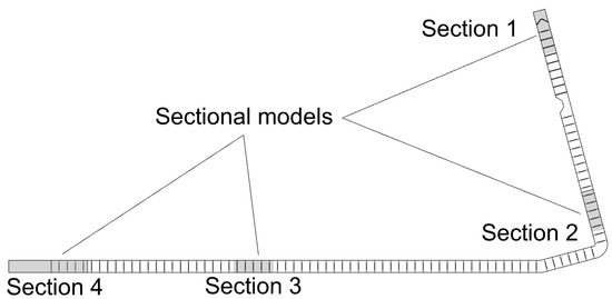
Figure 2.
Full fishway model, which corresponds with Sim1, and sectional model boundaries, which correspond with Sim2–Sim5.
3.1. Numerical Model
The model in the present study utilizes OpenFOAM version 8. The solver, interFoam, solves the discrete Reynolds-Averaged Navier–Stokes (RANS) equations for two incompressible, isothermal immiscible fluids using a volume-of-fluid (VOF) phase fraction-based interface capturing method. The governing equations using index notation and the Einstein summation convention are specified below, and additional information on its implementation may be found in [25]. The continuity equation is defined as:
and the momentum equation is defined as:
where is the velocity, is the gravitational acceleration, is the pressure, and are the viscose and turbulent stresses, is the surface tension, and is the density. For two-phase flows, the density is determined by:
where is equal to 1 inside the water volume with density and 0 inside the air volume with density . At the interface between the two fluids, the value of varies between 0 and 1. In addition to the continuity and momentum equations, an additional equation is solved for the interface between the two fluids:
The two equation realizable k-ε model is used for turbulence closure, which offers a more accurate calculation of turbulent viscosity on complex structures than the standard k-ε model. Detailed descriptions of the following equations are found in [26,27]. The transport equation for turbulent kinetic energy, , is expressed as:
and the transport equation for dissipation rate, , is expressed as:
where constant is determined by:
and , the mean strain, is:
The remaining constants are determined to be and , as prescribed in [26]. The effective diffusivity for and , are:
and the rate of strain tensor is defined as:
The turbulent viscosity is calculated using:
While the standard k-ε model assumes a constant for , the realizable k-ε model considers an experimentally derived formulation. A more detailed view of the formulation of can be found in [26,28]. In the present study, the density of water, , was assumed to be 1000 kg/m3, with a kinematic viscosity, , of 1 × 10⁻⁶ m2/s. The density of air was assumed to be 1.2 kg/m3, with a kinematic viscosity of 1.48 × 10⁻⁵ m2/s. Simulations were run on the Department of Defense (DoD) high-performance computing (HPC) system, JIM. Table 2 shows the discretization schemes and computational resources used to perform the simulations, which were run until a steady flow rate convergence was achieved in the outlet.
Table 2.
Discretization schemes and computational resources utilized for running the OpenFOAM simulations.
3.2. Numerical Mesh and Boundary Conditions
The numerical mesh was built using OpenFOAM’s built-in meshing utility, snappyHexMesh, which generates 3D meshes from hexahedral and split-hexahedral elements automatically from stereolithography (STL) files [29]. The mesh conforms to a surface by iteratively refining an initial background mesh and morphing the resulting split-hex mesh to the surface.
The background mesh is constructed by an additional built-in utility, blockMesh, which defines the size and orientation of the cells with eight arbitrarily placed vertices to form a hexahedron, referred to as a block [30]. Each block has a unique local coordinate system, allowing portions of the mesh to align with sloped or curved geometry. Multiple blocks with cells of varying curvatures and directions can then be merged to form a single continuous block assuming identical nodes and nodal spacing between blocks. Simpler domains often do not require this step, however, the size and complexity of the fishway necessitates a more complex construction of the blockMesh. Figure 3 contains the boundaries of the five blocks that were merged to construct Sim1. The target mesh spacing is 1.25 m × 1.25 m × 0.625 m, but the prescription of the spacing is limited by the curvature of the structure. For example, to merge block 3 with the surrounding blocks, the number of nodes in streamwise and spanwise directions must be identical and, therefore, the desired uniform cell spacing cannot be explicitly prescribed as cells near the smaller arc of the curve contain much more densely packed cells, as seen in Figure 3. Another limitation is seen in block 2, where a perfect hexahedron is not possible due to the fishway angle at 15°. As a result, the cell spacing within this block and subsequent blocks varies slightly from the target, since mesh spacing must be consistent throughout. The meshes in Sim2–Sim5 are constructed with a single block, however, the block boundaries from the full fishway model are reused and the cell spacing has been updated for a target mesh spacing of 0.625 m × 0.625 m × 0.625 m. Additional refinement for all the models was added near the bed, walls, weirs, and free surface. The meshes in Sim2–Sim5 contain four prismatic layers of cells near the bed, wall, and weir surfaces to improve the near-wall boundary layer resolution, and a detailed view of the mesh for Sim2 is shown in Figure 4. Numerical meshes for the remaining simulations are similarly constructed. A summary of the mesh information can also be found in Table 1.
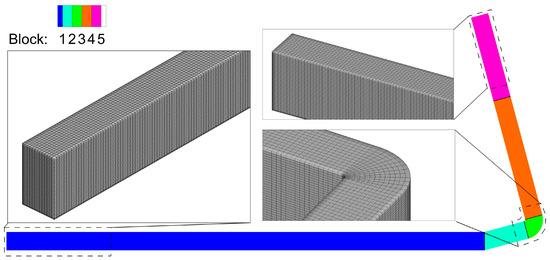
Figure 3.
Block boundaries defined in the blockMesh dictionary, which determine the cell sizing of the final mesh. Sections of the final merged block are shown and enlarged to show details of the cell direction and spacing.
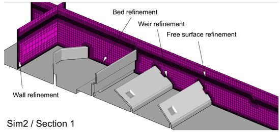
Figure 4.
Vertical slices through the computational volume show the mesh detail of Sim2. Sim1–Sim5 contain bed, wall, weir, and free surface refinement, and Sim2–Sim5 contain additional prismatic cell layers near the bed, weir, and wall surfaces.
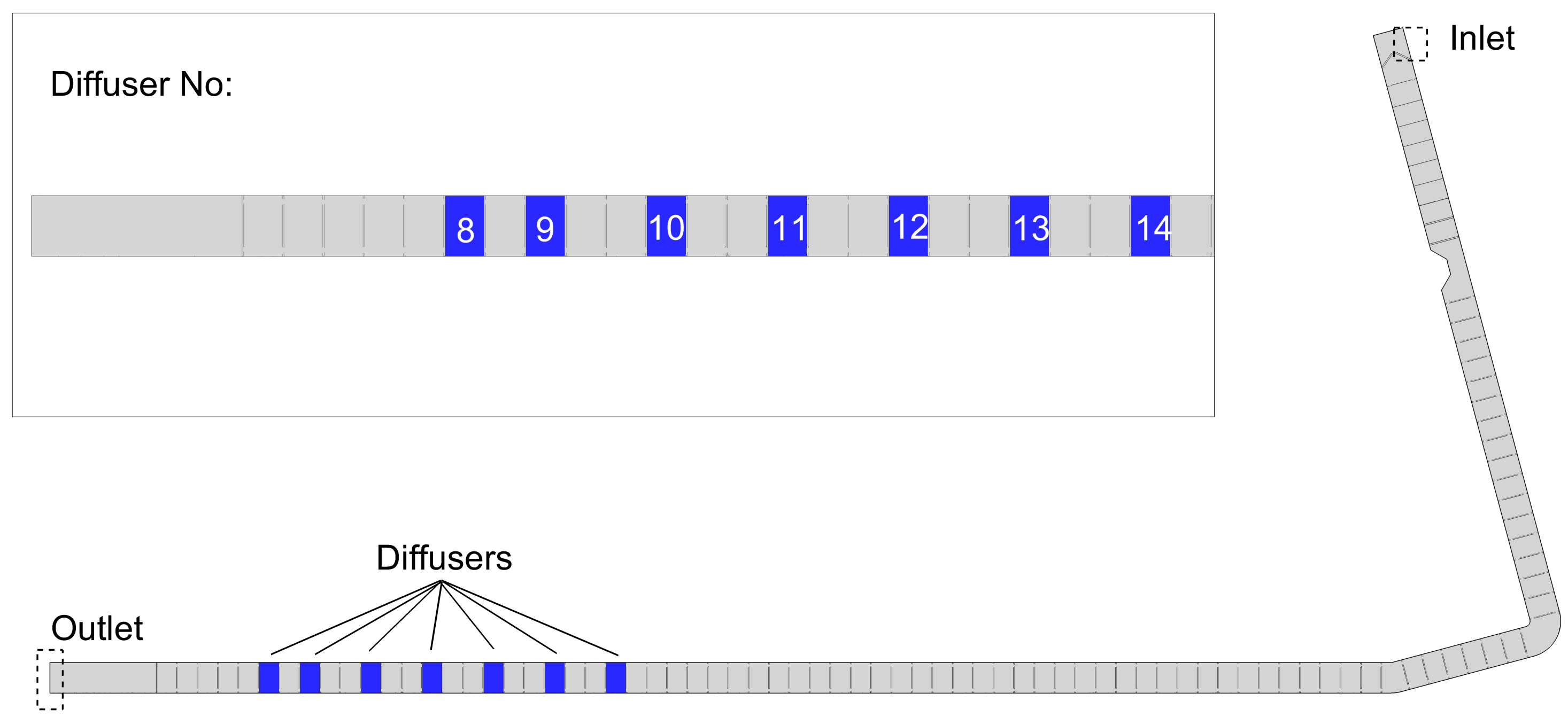
Boundary locations and diffusers for Sim1 are labelled in Figure 5. Each simulation contains inlet and outlet boundaries for the air and water phases, and the depth at each location is fixed to represent a fixed elevation of the pool and tailwater. The air boundaries (the top boundary and those above the water inlet and outlet) are considered inlet–outlet boundary conditions to allow free air flow. For Sim1, there are seven additional inlet boundaries, which represent the gravity-fed diffuser grates near the downstream end of the fishway. The flow rates to these boundaries are set using estimates based on the Bernoulli equation for gravity supply.

Figure 5.
Inlet, outlet, and diffuser boundary locations within Sim1. Diffusers are numbered in ascending order from downstream to upstream and are considered additional inlet boundaries.
3.3. Simulation Conditions
All the simulations consider the pool elevation as 103.3 m and the tailwater elevation as 81.1 m. For Sim1, the inlet discharge from the forebay is 5.56 m3/s, which is the 6-year average from 2012–2019, and the gravity-fed diffusers add an additional 19.88 m3/s near the downstream end of the fishway. Estimates for the individual diffuser flow rates can be found in Table 3, and Figure 5 shows the locations of the diffusers in the domain relative to the inlet and outlet. A flow rate of zero indicates that the diffuser is considered closed for this set of conditions and is not providing any additional flow. Boundaries that meet this condition are considered wall boundaries and a no-slip boundary condition is applied. The water depth in the tailrace is maintained by applying a fixed hydrostatic boundary condition at the outlet. For Sim2–Sim5, since the inlet boundary is located within an arbitrary section of the full fishway, the inlet conditions are set by extracting the nodal values at the same location within Sim1 and applying them directly to the inlet boundaries of Sim2–Sim5. The simulations were run until flow rate convergence was achieved at the model outlet. The boundary conditions for each variable are outlined in Table 4.
Table 3.
Gravity-fed diffuser flow rate estimates for additional diffuser inlet boundaries.
Table 4.
OpenFOAM boundary conditions for interFoam solver. Abbreviations: calc: calculated, eWF: epsilon wall function, ffP: fixed flux pressure, fRIV: flow rate inlet velocity, fV: fixed value, iO: inlet outlet, kRWF: kqR wall function, nkWF: nutk wall function, nS: no slip, tVMFV: time varying mapped fixed value, tP: total pressure, zG: zero gradient.
4. Simulation Results
4.1. Model Validation
Sim1 is used as the validation model. The symbols in Figure 6 show the computed water column depth above each weir in the fishway. The measured water column depth for each weir is reported to be 0.3 m and is represented by the dashed line. An iso-surface for a phase-volume fraction equal to 0.5 is used to represent the free surface. The depth was determined by subtracting the elevation of the free surface from the elevation of each weir near its crest. The first 17 weirs near the outlet sit in a region known as the backwater, where the water surface elevation is no longer changing due to the influence of the tailwater depth. Excluding these weirs, the predicted average water column depth is 0.3 m.
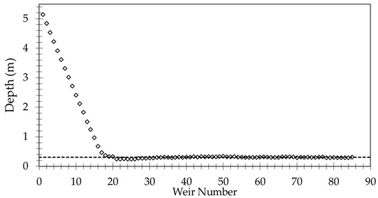
Figure 6.
Water column depth above each weir near the crest. Weirs are numbered in ascending order from downstream to upstream. Reported water column depth is represented by the dotted line.
4.2. Fishway Hydrodynamics
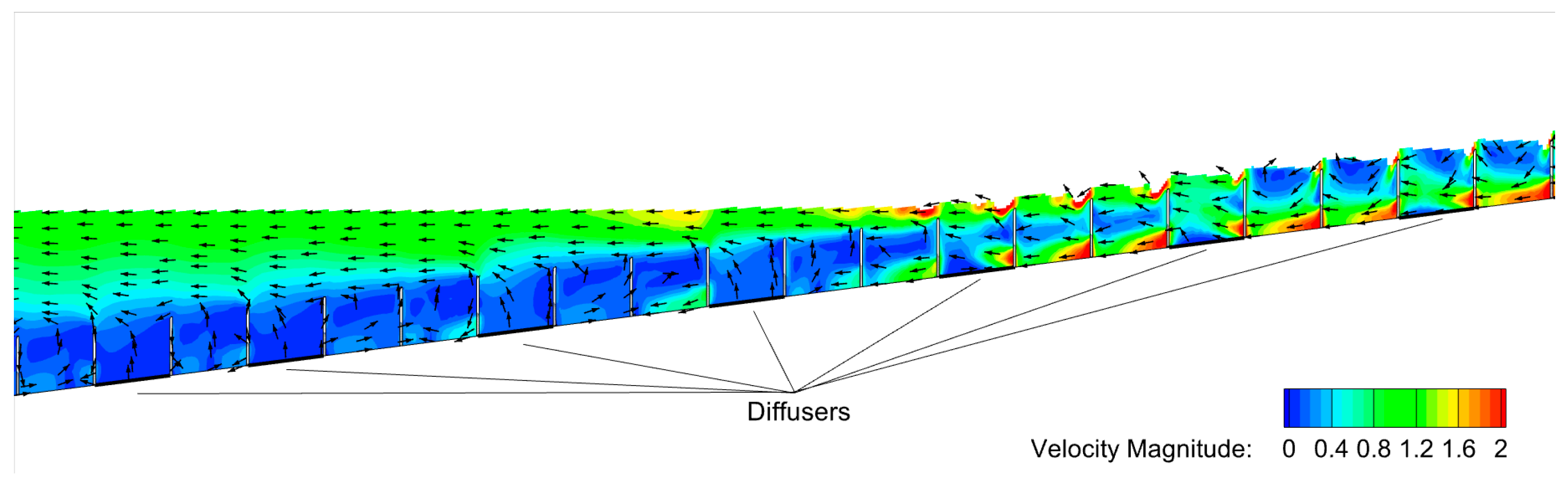
Highly complex hydrodynamic flow patterns are observed in the fishway. Near the inlet, the flow is regulated by the position of the regulating and tilting weirs, delaying large volumes of water from immediately entering the fishway and controlling the depth. In this area and approximately 80 m downstream, the fishway bed is flat, and flow through the tilting weirs is generally slow. As the fishway slopes downward, velocities begin to increase. Figure 7 shows the water surface and vertical slices through the water volume, colored by the velocity magnitude with vectors to indicate the direction of the flow. Vectors were interpolated in a coarse uniform grid for better visualization. Flow is fastest through the weir orifices, reaching up to 2.5 m/s in some regions, and the water depth over each weir provides brief jets of water on the free surface that reach up to 2 m/s, as seen by the iso-surface in Figure 7a. In the pool regions, as seen in the middle vertical slice in Figure 7b, the flow is characterized by recirculations and a flow less than 0.5 m/s, which provides relief to fish as they navigate through the fishway. Near the downstream end, diffusers add additional flow, but do not provide any significant change in the hydrodynamic flow patterns, as shown in Figure 8. This is likely because four of the seven diffusers sit in the backwater, and of the three that are not in the backwater, only one is currently operational.
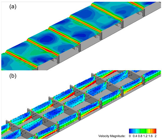
Figure 7.
The hydrodynamic field of a sloping section of the fishway with (a) an iso-surface of the phase-volume fraction to represent the water surface and (b) vertical slices through the water volume with uniform velocity vectors to show the complexity and direction of flow.

Figure 8.
A vertical slice through the fishway downstream end near the diffuser inlet boundaries contoured by the velocity magnitude with velocity vectors. Vertical scale is enlarged 2.5× for detail.
4.3. Mussel Risk Assessment
The risk assessment conducted in this study applies preference index curves (often referred to as habitat suitability curves) for the water depth, depth-averaged velocity, and wall shear stress outputs from the computational solutions. Continuous piecewise functions (found in [17]) were applied during post-processing to determine an index value (Idx) associated with each variable. The index ranges from 0 to 1, with 0 indicating no habitat suitability and 1 indicating the maximum habitat suitability. Depths between 1.5 m and 3.2 m, velocities between 0.19 m/s and 0.5 m/s, and wall shear stresses between 32.2 Pa and 74.7 Pa, are considered the highest risk and correspond to an index of 1.0.
This analysis is performed in two steps. Firstly, the solution from Sim1 is used to compute the preference index for the depth and depth-averaged velocity, since these variables do not require a high near-wall boundary layer resolution. These variables are not part of the standard output in interFoam, so MATLAB scripts were developed to parse each nodal value in the mesh and compute the water depth and averaged velocity quantities. Water depth is calculated using the elevation of the free surface (using a phase fraction of 0.5) and subtracting the elevation of the closest fishway bottom surfaces. Velocity is averaged over the water column depth. Secondly, the solutions from Sim2–Sim5 are used to compute the preference index for the wall shear stress, since this quantity extensively relies on a suitable boundary layer resolution. Shear stress is a standard output variable within interFoam, so no additional post-processing is required.
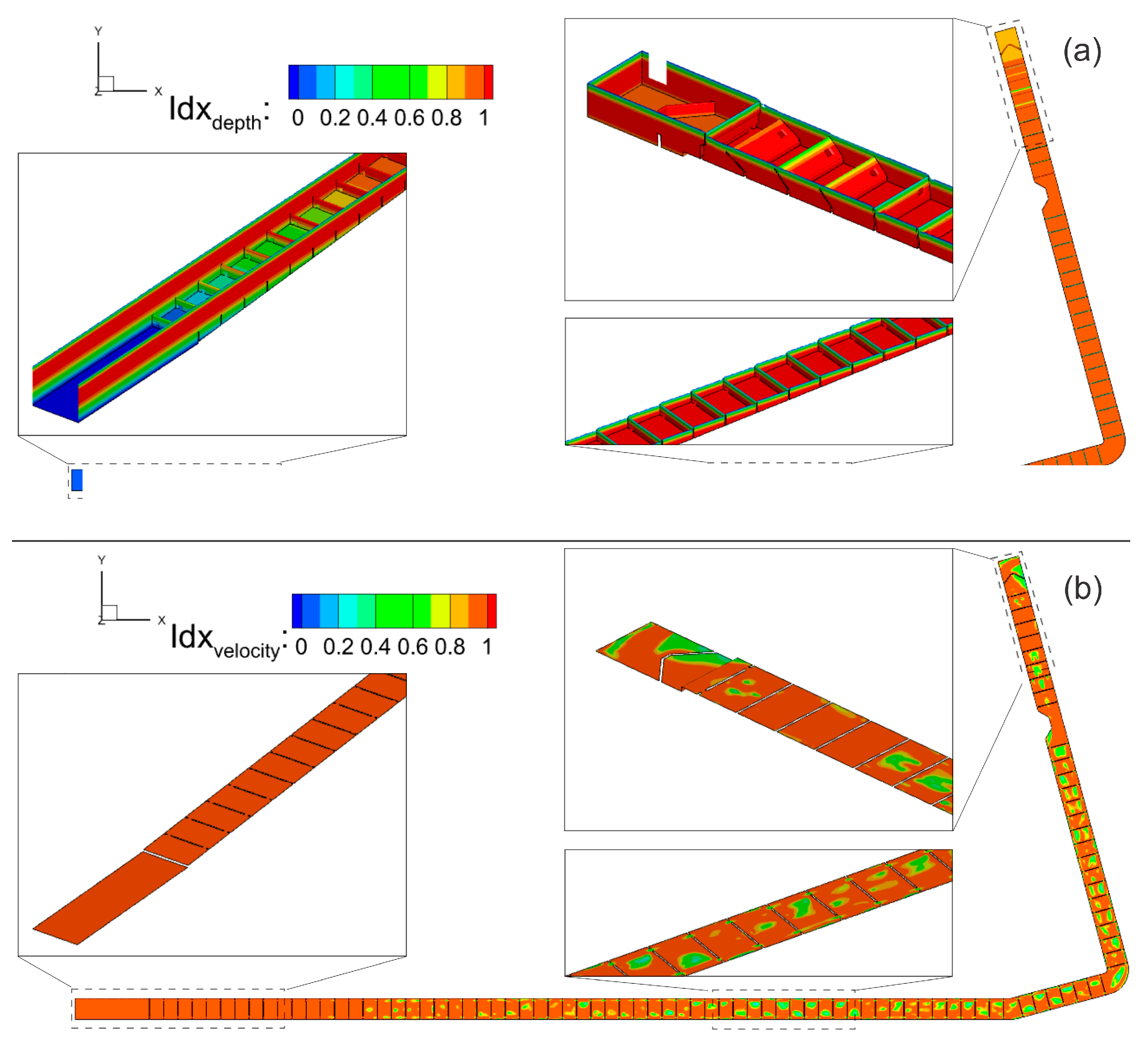
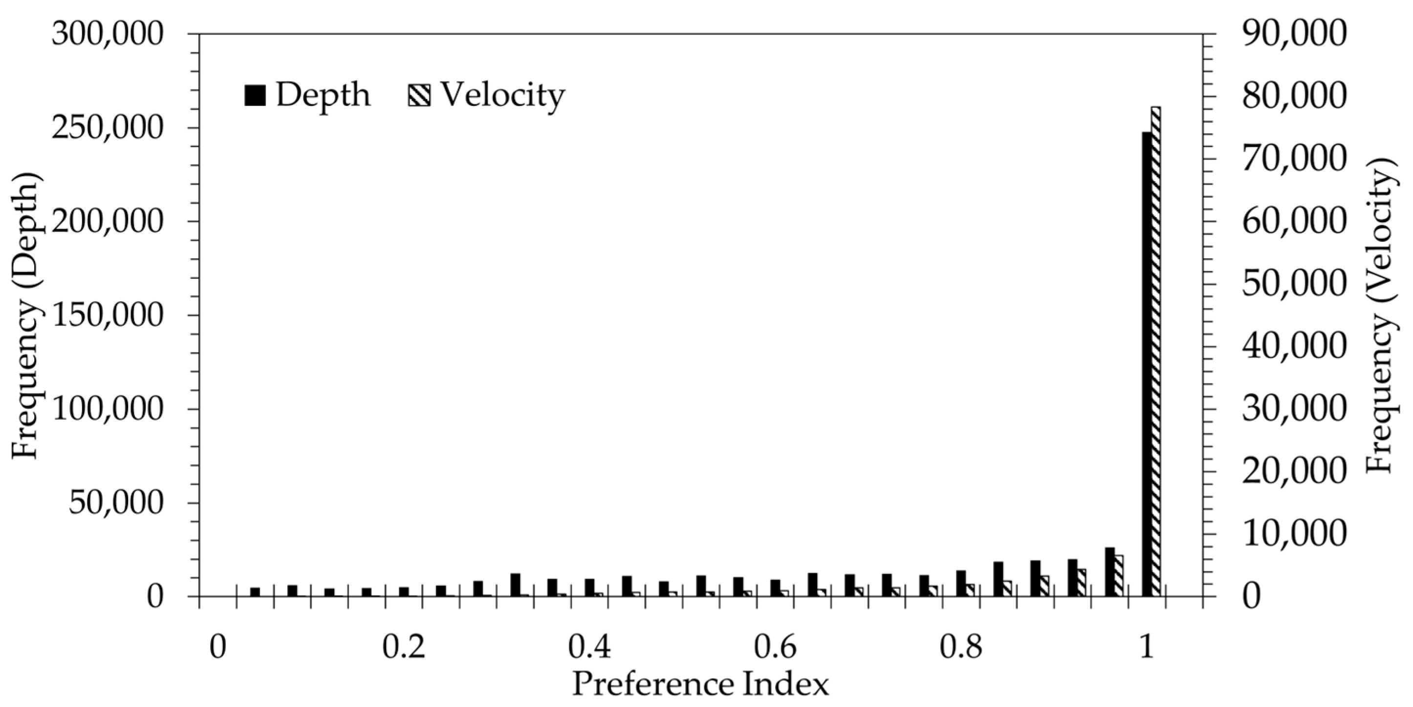
Figure 9 shows the preference index contours for the depth and velocity. For depth, which considers the weirs, walls, and diffuser boundaries, the preference index is between 0.825 and 0.85 in the area immediately near the inlet and increases to 1.0 for the entire fishway until the backwater region, where the water becomes deeper and ultimately reduces to 0 in the deepest region near the outlet (Figure 9a). There is an additional reduction in risk along the upper portions of the walls and weirs near the free surface. On average, the depth of the fishway bed is 2.21 m, with an average preference index of 0.83. As a 2D depth-averaged quantity, the preference index for velocity only considers non-vertical surfaces (i.e., the fishway bed and diffuser boundaries), and the preference index is 1.0 for the majority of the fishway, with some small reductions (though still reaching moderate risk) in the pool regions (Figure 9b). The average preference index is 0.93, and there is no reduction in the backwater region, such as in the solution for the depth index. Overall, when applied to depth and velocity, the preference index identifies significant risk in the majority of the ladder (see Figure 10).

Figure 9.
Contours of the preference index functions applied to the nodal values for (a) water column depth and (b) depth-averaged velocity variables for Sim1. Velocity contours exclude vertical surfaces.

Figure 10.
Preference index histogram for nodal values of water column depth and depth-averaged velocity for Sim1. Cell count for velocity excludes vertical surfaces.
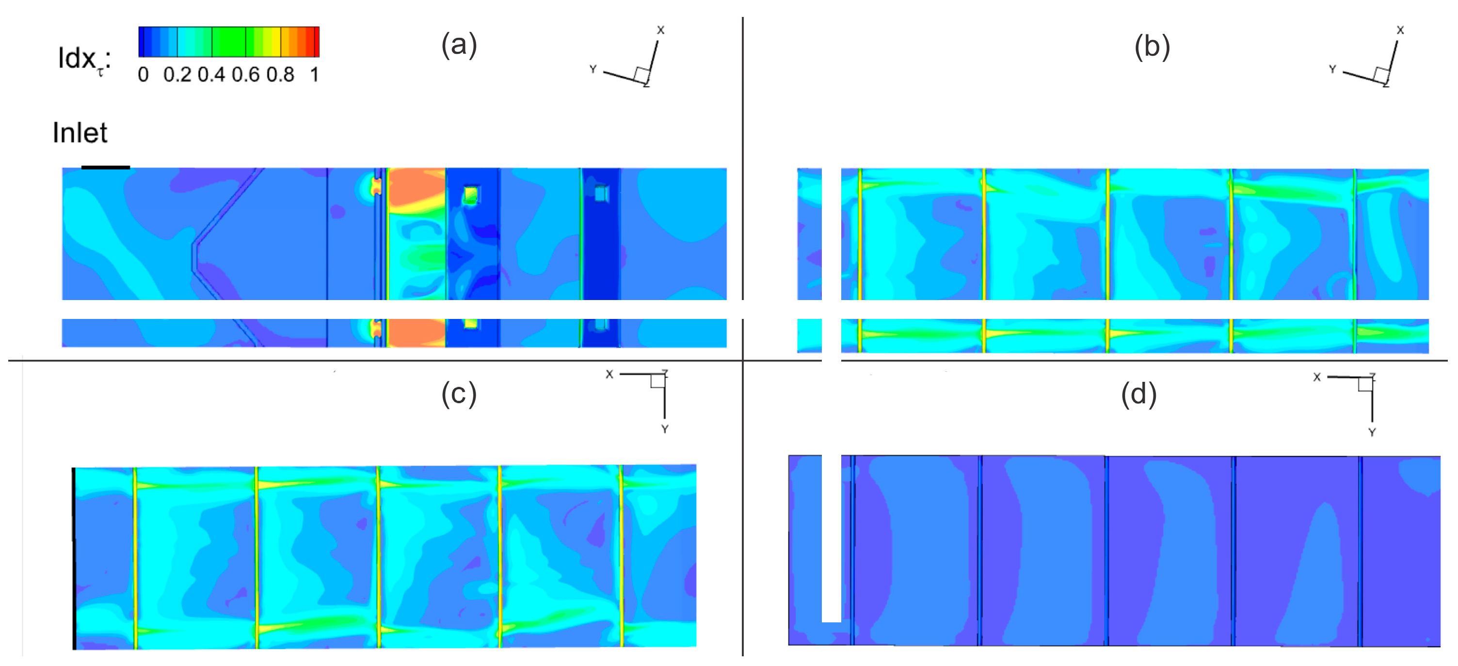
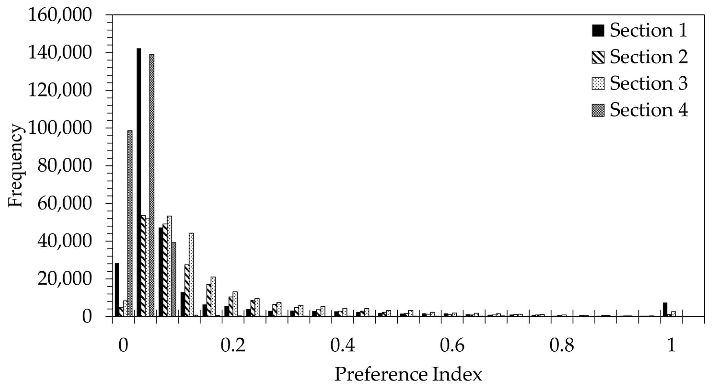
Figure 11 shows the preference index contours for the wall shear stress for Sim2–Sim5, and Figure 12 shows a histogram of the preference index. In contrast with the index values for depth and velocity, very few regions face a significant threat due to shear stress. Section 1 contains one region of concern near the orifice openings of the flow regulating the weir, but the extent is limited to a small region downstream of the orifices (Figure 11a). Section 2 and Section 3 contain no preference index higher than 0.7, with the highest occurring in the vicinity of the orifices (Figure 11b,c). Section 4 contains no regions of concern, with a maximum preference index no higher than 0.01 (Figure 11d). Still, the results indicate that downward sloping sections of the fishway are at moderate risk of mussel infestation, especially downstream of the orifices.
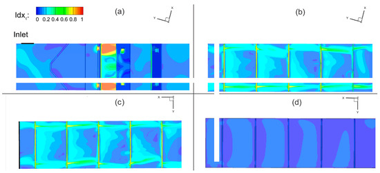
Figure 11.
Contours of the preference index functions applied to the nodal values for wall shear stress for: (a) Sim2, (b) Sim3, (c) Sim4, and (d) Sim5.

Figure 12.
Preference index histogram for nodal values of wall shear stress for the sectional models (Sim2–Sim4).
5. Discussion
According to the simulation results, there is a significant and consistent risk when considering both the depth and depth-averaged velocity in the fishway (see Figure 9). One potential issue with this approach is that in some regions of the fishway, particularly near the orifices, the velocity varies significantly in the water column, indicating that depth-averaging may not be an accurate representation of a three-dimensional hydrodynamic flow field. A more reasonable approach would be to determine the infestation preference for local velocity quantities, but no such analysis was found in the literature. On the other hand, when considering the risk due to shear stress, the majority of the fishway can be considered low risk, especially in the backwater region (see Figure 11). Some regions, particularly those within and just downstream of each orifice reach moderate risk, but these regions are limited in size.
When considering the totality of all the results, there are conflicting results depending on the variable in question and, thus, it is difficult to prescribe a risk level that encompasses the influence of all the variables. A better approach would be to make more general assessments of the expected risk in portions of the fishway. The backwater region poses the lowest risk overall, and the inlet section and all fishway walls and weirs, especially near the free surface, are at moderate risk. The remainder of the fishway poses a significant risk, with regions within and just downstream of the orifices having the highest risk overall due to the unique combination of depth, velocity, and shear stress.
If one or both fishways at McNary are fully colonized, extensive negative impacts on fish passage are expected. This is due, in part, to potential damage to the concrete structures if left untreated, but also due to the effects on fish interaction with Ice Harbor-type fishways. Fish either pass through the submerged weir orifices, or, if size and swimming ability permits, over the weir through the overtopping flow [23]. Once a fish passes through a stretch of the fishway, they utilize the slower regions of flow in the pool region to rest. Eventually, fish will either traverse the full length of the ladder and exit into the forebay or will return to the tailrace in the event of a failed attempt. Mussel colonization in the vicinity of weir orifices would be detrimental, affecting the overall efficiency of the fishway. While some studies have suggested that partial blockages of submerged orifices may lead to a minor improvement in fishway efficiency for shad and lamprey [31], efficiency for larger-bodied salmonids, which are the primary fish species passing through McNary, are likely to suffer due to their reliance on the submerged orifices. At maximum size, a colony might have the capacity to completely block the flow through the submerged orifices, significantly restricting fish passage.
It is important to remember, however, that the criteria for mussel colonization potential in [17] were determined for a specific habitat, which may not be entirely transferrable to the set of flow conditions in the present study. Very limited data is available on characterizing the relationship between colonization potential and hydraulic variables, and there is much room for improvement. Still, the preceding analysis provides a useful data-informed computational model, which is a first step in assessing mussel infestation potential and can be improved once sufficient habitat data becomes available.
6. Conclusions
In the present study, a computational model has been developed to investigate the impact of a potential Dreissena polymorpha infestation within the McNary Lock and Dam Oregon-shore fishway. A series of simulations were performed using the OpenFOAM solver interFoam to predict the flow pattern through the fishway at one pool and tailwater elevation. The model was validated using the measured water column depth over each weir. A two-phase flow model was critical in determining the location of the free surface, which allowed the accurate measurement of the water column depth over each weir as necessary for the validation. After validation, simulations were performed to determine the risk of Dreissena colonization based on the water depth, depth-averaged velocity, and wall shear stress, as prescribed in the literature for lotic systems. The results indicate that regions of the fishway in the backwater region are at the lowest risk of infestation, while regions between and just downstream of the weir orifices are at the highest risk. If a colony were to become established in these areas of concern, especially at the maximum potential colony size, fish passage may become delayed or impossible, in the most extreme case, due to the impact of orifice blockages on hydrodynamic flow patterns. While the analysis presented in this paper provides an initial estimate of the impact of Dreissena on the fishway, there are clear limitations due to data scarcity to correlate hydraulic variables with mussel colonization. To develop a more robust predictive tool, future work should focus on additional hydraulic data collection within the fishway, and data-driven relationships between Dreissena presence and key hydrodynamic variables.
Author Contributions
Conceptualization, D.L.S. and D.W.; methodology, D.L.S.; software, A.S., D.L.S. and M.P.; validation, A.S., D.L.S. and M.P.; formal analysis, A.S., D.L.S. and M.P.; resources, J.C.; writing—original draft preparation, A.S.; writing—review and editing, D.L.S. and M.P.; visualization, A.S. and M.P.; supervision, D.L.S.; project administration, D.L.S. and J.C.; funding acquisition, D.L.S. and J.C. All authors have read and agreed to the published version of the manuscript.
Funding
This research received no external funding.
Data Availability Statement
Data is available upon reasonable request.
Conflicts of Interest
The authors declare no conflicts of interest.
References
- Ludyanskiy, M.L.; McDonald, D.; MacNeill, D. Impact of the Zebra Mussel, a Bivalve Invader. Bioscience 1993, 43, 533–544. [Google Scholar] [CrossRef]
- O’Neill, C.R. The Zebra Mussel: Impacts and Control; NOAA: Silver Spring, ML, USA, 1997; ISBN 6072552080. [Google Scholar]
- Ackerman, J.D.; Cottrell, C.M.; Ethier, C.R.; Allen, D.G.; Spelt, J.K. Attachment Strength of Zebra Mussels on Natural, Polymeric, and Metallic Materials. J. Environ. Eng. 1996, 122, 141–148. [Google Scholar] [CrossRef]
- Athearn, J. Risk Assessment For Adult and Juvenile Fish Passage Facilities on the Mainstem Lower Snake and Lower Columbia Rivers Relative to a Potential Zebra Mussel Infestation; US Army Corps of Engineers, Northwest Division: Portland, OR, USA, 1999; pp. 1–12. [Google Scholar]
- Rajagopal, S. Effects of Temperature, Salinity and Agitation on Byssus Thread Formation of Zebra Mussel Dreissena Polymorpha. Neth. J. Aquat. Ecol. 1996, 30, 187–195. [Google Scholar] [CrossRef]
- Neilson, F.M.; Theriot, E.A. Components of Navigation Locks and Dams Sensitive to Zebra Mussel Infestations; US Army Engineer Waterways Experiment Station: Vicksburg, MS, USA, 1992. [Google Scholar]
- USACE Portland District; USACE Walla Walla District. Annual Fish Passage Report 2022: Columbia and Snake River Projects; USACE Portland District: Portland, OR, USA, 2022. [Google Scholar]
- Drake, J.M.; Bossenbroek, J.M. The Potential Distribution of Zebra Mussels in the United States. Bioscience 2004, 54, 931–941. [Google Scholar] [CrossRef]
- Wells, S.W.; Counihan, T.D.; Puls, A.; Sytsma, M.; Adair, B. Prioritizing Zebra and Quagga Mussel Monitoring in the Columbia River Basin; Center for Lakes and Reservoirs Publications and Presentations: Portland, OR, USA, 2011; Volume 10. [Google Scholar]
- Whittier, T.R.; Ringold, P.L.; Herlihy, A.T.; Pierson, S.M. A Calcium-based Invasion Risk Assessment for Zebra and Quagga Mussels (Dreissena Spp.). Front. Ecol. Environ. 2008, 6, 180–184. [Google Scholar] [CrossRef]
- Phillips, S.; Darland, T.; Sytsma, M. Potential Economic Impacts of Zebra Mussels on the Hydropower Facilities in the Columbia River Basin; Pacific States Marine Fisheries Commission: Portland, OR, USA, 2005. [Google Scholar]
- O’Neill, C.R.; Dextrase, A. The Introduction and Spread of the Zebra Mussel in North America. In Proceedings of the Fourth International Zebra Mussel Conference, Madison, WI, USA, 7–10 March 1994; pp. 433–446. [Google Scholar]
- de Kozlowski, S.; Page, C.; Whetstone, J. Zebra Mussels in South Carolina: The Potential Risk of Infestation; NOAA: Silver Spring, ML, USA, 2002. [Google Scholar]
- USACE Fort Worth District. Zebra Mussel Resource Document; USACE Fort Worth District: Trinity River Basin, TX, USA, 2013. [Google Scholar]
- Horvath, T.G.; Crane, L. Hydrodynamic Forces Affect Larval Zebra Mussel (Dreissena Polymorpha) Mortality in a Laboratory Setting. Aquat. Invasions 2010, 5, 379–385. [Google Scholar] [CrossRef]
- Rehmann, C.R.; Stoeckel, J.A.; Schneider, D.W. Effect of Turbulence on the Mortality of Zebra Mussel Veligers. Can. J. Zool. 2003, 81, 1063–1069. [Google Scholar] [CrossRef]
- Sanz-Ronda, F.J.; López-Sáenz, S.; San-Martín, R.; Palau-Ibars, A. Physical Habitat of Zebra Mussel (Dreissena Polymorpha) in the Lower Ebro River (Northeastern Spain): Influence of Hydraulic Parameters in Their Distribution. Hydrobiologia 2014, 735, 137–147. [Google Scholar] [CrossRef]
- Jasak, H. OpenFOAM: Open Source CFD in Research and Industry. Int. J. Nav. Archit. Ocean Eng. 2009, 1, 89–94. [Google Scholar] [CrossRef]
- Fuentes-Pérez, J.F.; Quaresma, A.L.; Pinheiro, A.; Sanz-Ronda, F.J. OpenFOAM vs FLOW-3D: A Comparative Study of Vertical Slot Fishway Modelling. Ecol. Eng. 2022, 174, 106446. [Google Scholar] [CrossRef]
- Santos, H.A.; Pinheiro, A.P.; Mendes, L.M.M.; Junho, R.A.C. Turbulent Flow in a Central Vertical Slot Fishway: Numerical Assessment with RANS and LES Schemes. J. Irrig. Drain. Eng. 2022, 148, 04022025. [Google Scholar] [CrossRef]
- Fuentes-Pérez, J.F.; Silva, A.T.; Tuhtan, J.A.; García-Vega, A.; Carbonell-Baeza, R.; Musall, M.; Kruusmaa, M. 3D Modelling of Non-Uniform and Turbulent Flow in Vertical Slot Fishways. Environ. Model. Softw. 2018, 99, 156–169. [Google Scholar] [CrossRef]
- Deshpande, S.S.; Anumolu, L.; Trujillo, M.F. Evaluating the Performance of the Two-Phase Flow Solver InterFoam. Comput. Sci. Discov. 2012, 5, 014016. [Google Scholar] [CrossRef]
- Eder, K.; Thompson, D.; Caudill, C.; Loge, F. Video Monitoring of Adult Fish Ladder Modifications to Improve Pacific Lamprey Passage at the McNary Dam Oregon Shore Fishway, 2010; University of California, Davis: Davis, CA, USA, 2011. [Google Scholar]
- McNary Lock & Dam Oregon Shore Fishway. Google Earth. Available online: https://earth.google.com/web/@45.9248124,-119.29721291,172.58102766a,0d,35y,8.4896h,80.087t,0r (accessed on 10 May 2024).
- Heyns, J.A.; Oxtoby, O.F. Modelling Surface Tension Dominated Multiphase Flows Using the VOF Approach. In Proceedings of the 6th European Conference on Computational Fluid Dynamics, ECFD, Barcelona, Spain, 20–25 July 2014; pp. 7082–7090. [Google Scholar]
- Shih, T.-H.; Liou, W.W.; Shabbir, A.; Yang, Z.; Zhu, J. A New K-Epsilon Eddy Viscosity Model for High Reynolds Number Turbulent Flows. Comput. Fluids 1994, 24, 227–238. [Google Scholar] [CrossRef] [PubMed]
- Shaheed, R.; Mohammadian, A.; Kheirkhah Gildeh, H. A Comparison of Standard k–ε and Realizable k–ε Turbulence Models in Curved and Confluent Channels. Environ. Fluid Mech. 2019, 19, 543–568. [Google Scholar] [CrossRef]
- Shih, T.H.; Zhu, J.; Lumley, J.L. A New Reynolds Stress Algebraic Equation Model. Comput. Methods Appl. Mech. Eng. 1995, 125, 287–302. [Google Scholar] [CrossRef]
- Mesh Generation with the SnappyHexMesh Utility. Available online: https://www.openfoam.com/documentation/user-guide/4-mesh-generation-and-conversion/4.4-mesh-generation-with-the-snappyhexmesh-utility (accessed on 9 April 2024).
- Mesh Generation with the BlockMesh Utility. Available online: https://www.openfoam.com/documentation/user-guide/4-mesh-generation-and-conversion/4.3-mesh-generation-with-the-blockmesh-utility (accessed on 9 April 2024).
- Haro, A.; Kynard, B. Video Evaluation of Passage Efficiency of American Shad and Sea Lamprey in a Modified Ice Harbor Fishway. N. Am. J. Fish. Manag. 1997, 17, 981–987. [Google Scholar] [CrossRef]


Disclaimer/Publisher’s Note: The statements, opinions and data contained in all publications are solely those of the individual author(s) and contributor(s) and not of MDPI and/or the editor(s). MDPI and/or the editor(s) disclaim responsibility for any injury to people or property resulting from any ideas, methods, instructions or products referred to in the content. |
© 2024 by the authors. Licensee MDPI, Basel, Switzerland. This article is an open access article distributed under the terms and conditions of the Creative Commons Attribution (CC BY) license (https://creativecommons.org/licenses/by/4.0/).