Abstract
Rapid socioeconomic development, urbanization, agricultural activities, and infrastructure development can greatly alter natural landscapes and their environmental impacts. Understanding these changes is crucial for more sustainable, integrated land management, including addressing water-related environmental challenges. In this study, we explored the impacts of two key factors on water quality and ecosystem services (ESs): land use change and the expansion of wastewater treatment (WWT) infrastructure by combining cellular automata Markov (CAM), water quality and environmental valuation modeling, and statistical analyses. We examined historic land use changes and forecasted their future evolution. The impacts were assessed by analyzing the spatial and temporal distribution of major water pollutants, water quality trends, and the economic valuation of ESs under real WWT expansion conditions, assessing a Chinese policy in effect. The Yongding River Basin in North China was selected as a case study due to significant urbanization and WWT changes over the past decades under arid conditions. The results indicate that pollutant loads were highest in urban areas, followed by rural areas, and that domestic WWT efficiency is a dominant factor in the spatial pattern of pollutant discharge. ES values decrease in the short term but can increase in the long term with WWT expansion, owing to the planned ecosystem restoration policy. This study provides valuable insights into the responses of water pollution and ESs to land use changes over spatiotemporal scales, encouraging the consideration of these factors in future land and infrastructure planning.
1. Introduction
In recent decades, rapid economic development has come at a significant cost to the natural environment [1]. A typical example of this effect is seen in China. As the world’s largest developing country, it is experiencing fast urbanization and industrialization and is facing serious environmental challenges [2]. The deterioration of surface water quality has emerged as the most serious environmental threat to water safety and ecosystem services (ESs) in the country. Despite some local improvements in inland waters’ condition [3,4], the overexploitation of water resources and extensive urbanization are persistently obstructing efforts to improve water quality [4,5]. While previous research has studied water quality trends, they are rarely associated with other parameters, such as land use changes, ecosystem factors, and environmental policies.
Changes in land use patterns can significantly impact water quality and ecological integrity, including ESs [6,7,8]. Incorporating these factors into sustainable land use planning, decision-making, best management practices, and optimal investment allocation is crucial [9,10], as it enables decision-makers to consider the interconnected effects of human activities on land, water, and the economy, promoting better environmental and economic outcomes [11,12,13]. The effects of land use changes (often driven by fast urbanization) on water resources have been explored in the literature. Salem et al. [14] assessed the impact of land use changes on groundwater recharge and groundwater levels in a floodplain using water balance and groundwater flow models. Blyth et al. [15] discuss recent advances in land surface modeling, including the need to better represent the effects of land use changes, and water management activities. The most common technique to simulate and forecast future land use is cellular automata Markov (CAM) modeling [16,17] through gridded geographic information system (GIS) technology [18,19]. Given that global land use change has affected almost a third of the global land area from 1960 to 2019, especially in developing regions [20], it is crucial to explore the future implications on the spatiotemporal patterns of water quality and pollutant discharge [21]. Several studies have investigated the negative impacts of land use changes, especially urbanization, on water quality. It is recognized that pressures like population growth, increased water demands, expansion of impervious areas, and a lack of proper sanitation infrastructure negatively impact urban water security and quality [22]. Depending on the land uses that are “replaced” by urban, industrial, or agricultural activities, different levels of water pollutants can be observed [23,24]. Such impacts are usually studied spatially through remote sensing techniques or regression models. Another aspect worth exploring is the mapping of the economic value of land use changes based on the ESs they can provide. ESs are closely linked to land use changes [9], and the importance of mapping them to achieve more integrated land use planning based on their sustainable provision is recognized [25,26]. The most common approach for this task is value transfer, as it can provide straightforward and reproducible estimates [27,28]. Value transfer involves applying economic values derived from one study area to another context to estimate the economic value of ESs [29]. Integrated assessments that consider ES values, especially in relation to land use changes and their future evolution, are rare but crucial for strategic planning, decision-making, and optimal investment allocation [30,31].
However, the connection between land use changes and their future evolution, water quality, and economic implications (through ESs) spatially has not been explored so far in a single assessment, to our knowledge. This paper aims to fill that gap while also considering the potential effects of human interventions, such as wastewater treatment plants’ (WWTPs’) expansion. A water-scarce region in North China is selected to better showcase the trade-offs and/or effects of land use evolution and water quality in developing areas, which often struggle to capture such interactions in policy-making and development planning [32,33]. The novelty of this study lies in the holistic approach followed, combining land use, water quality, ESs, and policy evaluation modeling (spatially and over time), considering socioeconomic development (in terms of population and socioeconomic growth), in the context of developing regions with arid conditions.
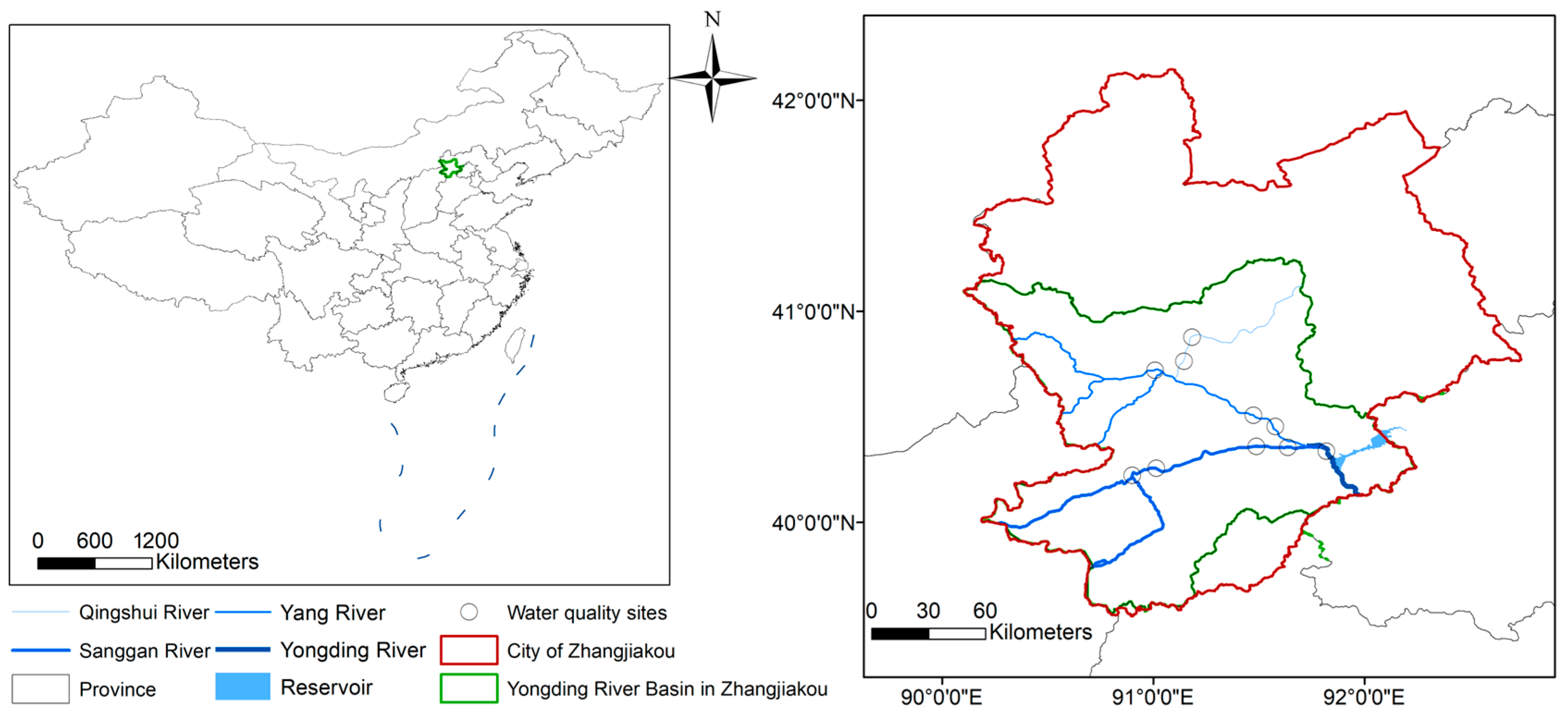
2. Study Area
The Yongding River Basin (YRB) is located in North China and has been selected as a case study to assess the responses of surface water quality and ESs to land use changes. The Yongding River is formed by the confluence of two major tributaries, the Sanggan River and the Yang River, creating a large basin of 47,000 km2 [34]. Our study area is part of the YRB in Zhangjiakou City, Hebei Province (the host city of the 2022 Winter Olympics), covering an area of 17,355 km2, which accounts for 47.5% of Zhangjiakou’s total area (Figure 1). This region is a developing area undergoing intensive urbanization. It has a semi-arid climate with an annual precipitation of 406 mm, and it is recognized as one of the most water-deficient areas in China, with natural water resources of only 203 m3 per capita per year, well below the absolute water scarcity threshold of 500 m3 per capita per year [35]. Numerous studies have shown that water quality deterioration, groundwater depletion, and natural runoff decrease are the main environmental issues in this region [36,37]. Over the past 30 years, dam construction and excessive water abstraction have significantly altered the YRB’s hydrology, causing the river to dry up, which was also due to the combined impacts of the arid climate and the overexploitation of water resources [37]. Persistent water shortages continue to hinder efforts to control pollution and improve water quality [38,39].
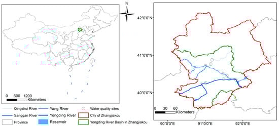
Figure 1.
The study area with the Yongding River in Zhangjiakou City, with the locations of the 10 water quality monitoring sites used for the period 2005–2019.
Currently, anthropogenic sources, such as chemical oxygen demand (COD), ammonium (NH4+), and total phosphorus (TP), are the major pollutants responsible for impaired surface water quality [36]. COD is a measure of the amount of oxygen that chemical pollutants consume during the decomposition of organic matter. Urban runoff, especially from areas lacking proper sewage treatment facilities, can also contribute to high levels of organic contaminants. Also, industries such as chemical manufacturing, food processing, and textiles often discharge high amounts of organic pollutants. NH4+ primarily comes from domestic sewage and waste, especially when WWT is not fully effective. It also originates from certain industries, such as chemical and fertilizer manufacturers and petrochemical plants. Rural areas are, in general, large contributors of TP due to extensive agricultural activities. However, TP can also result from urban runoff including domestic detergents. Additionally, industrial effluents can contain phosphorus, especially those from industries involved in metal finishing, food processing, and chemical manufacturing.
Previous research has primarily focused on temporal variations in pollutant concentrations and water resource availability [40,41,42], often overlooking direct connections to land use changes and efforts to restore river water quality. For the water quality assessment in this study, 10 water quality monitoring sites were used, covering 15 years of water quality monitoring records [38] (Figure 1).
The YRB is a unique case featuring a combination of water scarcity conditions (aridity), water quality issues, significant population and socioeconomic growth, including rapid urbanization and industrialization, and regulatory-supported water infrastructure development. This situation allows us to study the interaction of these factors with land use changes, environmental economics, and policy considerations.
3. Methods
3.1. CAM Model for Land Use Change Forecast
Based on historical changes in land use, the CAM model approach, which incorporates a cellular automata (CA) module and a Markov-chain process, can forecast future land use changes at a spatial level (e.g., pixels/cells on a map). This approach relies on a transition probability matrix, which indicates the likelihood of each cell (pixel) transitioning from one land use type X in year t to another land use type Y in year t + 1. The Markov module predicts quantitative land use changes, while the CA module simulates the spatial distribution of these changes [16,17]. The CAM model generates transfer probability matrices and suitability maps for different land use categories to inform future projections.
For this task, the software IDRISI Selva 17 from the Clark Lab platform was applied [43]. The input data included a digital elevation model (DEM), maps of conservation areas where development is restricted, urban extent maps, and transportation data from 2000, 2005, and 2015. The land use grid had a resolution of 90 × 90 m, enabling detailed (fine-resolution) simulations. We used the YRB in Zhangjiakou City as the study area boundary (Figure 1). The simulation process comprised four main steps: Firstly, the Markov chain generated a transfer matrix using land use classifications from 2000 and 2005 in IDRISI. Secondly, we determined the suitability of land use types for potential transformations based on socioeconomic drivers (represented by the transportation network) and physical/topographic factors (DEM, slope, etc.), using the multi-criteria evaluation method within IDRISI. Thirdly, we produced suitability maps for each land use type, which, together with the transfer matrix, informed the forecasted land use map for 2015. Finally, after error checking and correction based on observed land uses in 2015, we projected land use maps for 2025 and 2035 (the end of our study period).
3.2. Estimating Discharges Causing Water Pollution
Next, we assessed the amount of pollutants (COD, NH4+, TP) entering the river network by taking into account their discharge from different point sources (domestic, service, industry, and captive breeding) and the diffusion sources based on the production and output coefficients. The detailed data used are provided in Table S1 in the Supplementary Materials. The pollutant discharge loads are mainly influenced by urbanization rate, investment in environmental protection funding (such as WWTP coverage), their efficiency (e.g., technologies used for treatment), as well as the WWTPs’ capacities. Considering these factors, we estimated the pollutants’ discharge into the river network from six sources, as shown in Equation (1).
PD is the total pollutants discharged into the river network. ULP and RLP are the amounts of pollutants from urban residents and rural residents after treatment in rural centralized WWTP facilities, respectively. The information on 16 WWTPs, e.g., treatment capacities and efficiencies, was collected from the Environmental Statistical Yearbooks of Zhangjiakou City, China. AP is the amount of pollutants from agriculture including farmland export from surface runoff, captive livestock, and poultry breeding discharges. IP is the amount of industrial pollutants, TIP is the amount of tertiary industrial pollutants, and UNP is the amount of urban non-point source pollutants. In this work, the related data on the pollutant load of major industries and urban and rural residents were collected from the environmental quality statistical yearbooks and the second national survey of pollution sources (Tables S1 and S2).
To estimate the water pollution associated with the different land use types spatially, a “district” unit was used to create a spatial grid consisting of the different activities/pollution sources described above. The district is the smallest administrative unit, where urban residents and rural residents are the control variables to calculate and allocate the population coefficient of each grid cell. Within this grid (size of 450 × 450 m), a mix of different activities can be captured to give an accurate spatial depiction of pollutant discharges per land use, based on the corresponding coefficients (Supplementary Materials, Equations (S1)–(S7)). Depending on the pollutant load of each district (Equation (1)), we synthesized the spatial pattern of the pollutant loads. The inflow of river water pollutants is estimated by considering domestic (Equation (2)), industrial (Equation (3)), services/tertiary industries (Equation (4)), pollution from the planting process (planting) (Equation (5)), livestock and poultry (Equation (6)), and urban non-point (Equation (7)) pollution sources.
Inflow of pollutants from domestic sources:
where is the inflow of pollutants from living sources of j grid in district i; is the inflow from rural residents of district i; is the inflow of urban residents of district i; n is the number of grids in district i; and are the rural population and urban population coefficients of grid j, respectively.
Inflow of pollutants from industrial sources:
According to the inflow pollutants from the different industries, the gridded industrial inflow pollutant was calculated as follows:
where is the inflow amount of industrial pollutants of grid j of district i; is the inflow amount of industrial pollutants of district i; is the urban land use coefficient of grid j. In this study, the industrial pollution load only came from urban land.
Inflow of pollutants from service sector sources:
where is the inflow amount of pollutants from the added value of the tertiary industry of grid j of district i; and are the inflow amounts of pollutants from the tertiary industry in rural and urban areas, respectively, of district i. is the coefficient of the tertiary industry from the rural area and of grid j, is the coefficient of the tertiary industry from the rural area and of grid j.
The inflow of TP from planting source:
where is the inflow amount of pollutants from the planting of grid j of district i; is the inflow amount of pollutants of district i, t; is the farmland coefficient of grid j. In this study, the pollution load of planting only came from farmland.
The inflow of pollutants from captive livestock and poultry breeding sources:
According to the scale of livestock and poultry breeding enterprises and the pollutant discharge amount, the gridded inflow density of the pollutants of livestock and poultry breeding was calculated as follows:
where is the amount of pollutants from livestock and poultry breeding of grid j of district i, t; is the amount of pollutants from livestock and poultry breeding of district i, t; is the rural land use coefficient of grid j. We consider the production of pollutants that occur during the lives of livestock and poultry. In the studied region, the current large-scale livestock and poultry breeding manure is almost all dry-treated and converted into organic fertilizer, and the pollutants discharged from breeding only come from the scattered feeding of livestock and poultry on rural land.
The inflow of pollutants from urban non-point sources:
where is the inflow amount of pollutants from urban land in grid j of district i, and is the urban land use coefficient of grid j. The detailed calculation process of these coefficients and the related data on population and GDP (Figure S1) are shown in the Supplementary Material and are based on our previous work [38].
3.3. Spatial Valuation of Ecosystem Services (ESs)
The changes in land use also result in changes in the economic value of landscapes, along with the provision of ESs. Currently, there is increasing momentum in valuing ESs when studied alongside land use changes, as the value of such analyses is increasingly recognized [12,44]. Costanza et al. (1997) [45] developed a robust method for estimating the global economic values of ESs based on the existing literature and original calculations for 17 ESs from 16 biomes [46,47].
The most straightforward way to apply this method to estimate the ES value (ESV) is to compare the 16 biomes identified by Constanza et al. [45] and assign their valuation coefficients to the respective land cover category [48] (Table 1; Equation (8)).
where is the area of the land use category, and the ES value coefficient () can be seen in Table 1. In this study, we estimated the ES value coefficients for the historical year (2015) and the forecasted years (2025, 2035) to assess the spatial changes in the value of ESs in the study area. The differences between the specific years can be estimated as shown in Equation (9):
where t0 and t1 are the starting year and final year, respectively, and T is the study period.

Table 1.
Biome equivalents for the seven land use categories and their corresponding ecosystem values [44,45].
3.4. Considering the Effects of Water Pollution Control Interventions
As mentioned, the main factors influencing water quality are related to treatment coverage, efficiency, and capacity; in other words, the ability to reduce pollutant loads before they reach water bodies. In this regard, the National Development and Reform Commission of China released a policy in 2016 titled “Overall Plan of Comprehensive Management and Ecological Restoration of Yongding River” (hereafter OPR—overall plan for restoration) [49]. The aim was to restore the Yongding River ecosystem and its urban livability by addressing water pollution, reducing pollutant discharges into water bodies, and improving surface water quality. This policy proposed a water pollution control target by assuming the expansion of WWTPs and the improvement in their treatment efficiency by 2035 (Table S2).
In this study, we also account for the effect of this policy on the 2035 time horizon as part of our discussion on the role of WWTPs (Section 5.3). This is achieved by integrating the forecasted land uses, the projected population and economic conditions based on GDP (Figure S1), and the assumed WWTP expansion and improvement, as outlined in the studied policy. Thus, combining these inputs, we estimate the future pollutant discharge and its spatial load distribution by applying the methods described in Section 3.2. In order to better illustrate the effect of the WWTPs and compare the results, we present the spatial distribution of the pollutants in Section 4.2, with a stable WWT efficiency (2017 values of Table S2), and in Section 5.3, where we discuss the role of the WWTPs, we use the updated WWT efficiencies of Table S2 for 2025 and 2035.
4. Results
4.1. Land Use Change Forecast
Following the CAM model, as described in Section 3.1, the land use changes were produced from 2015 (calibration and validation year) until 2035 (Figure 2). The simulated and actual land use maps of 2015 in this region were compared using the “validate” module in IDRISI. Unlike the traditional Kappa statistic, which is commonly used for such analyses, the validate module breaks the validation down into several components with associated statistical results [50]. This module provides the quantitative errors and spatial location errors, including chance agreement, quantity agreement, grid cell agreement, quantity disagreement, and grid cell disagreement, for the simulation of land use accuracy assessment based on the quantity and location of each land use type [16]. The simulation error rate is lower than 20%, the agreement quantity is higher, and the disagreement grid cell is lower than some published results [16,51] (Table 2).
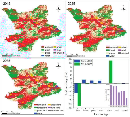
Figure 2.
The modeled land use change maps for the YRB in Zhangjiakou city in a ten-year step from 2015 to 2035, and the quantified changes per land use type during the study period.
Table 2.
The accuracy analysis of land use prediction (land area: km2).
The results indicate that the majority of future urban areas will grow around the existing urban areas. From 2015 to 2035, the urban area in Zhangjiakou will increase significantly by 20.8% (from 540.89 km2 to 653.16 km2). This is attributed to the continuous increase in urbanization and socioeconomic development [52]. Historically, the region has been subject to water overexploitation resulting in a continuously diminishing area of water bodies, especially after 2000 [37]. As part of the broader restoration efforts and water conservation and protection plans of the region, the OPR policy sets the target of gradually restoring the water body area, reaching 2000 levels by 2025 [53]. The land use change forecast also takes into account the OPR policy, and the previously reduced water areas are assumed to increase from 285.32 km2 in 2015 to 298.60 km2 in 2025. After 2025, the water area is projected to remain constant, as, according to the OPR policy, any change in the water areas into other land use types will be prohibited [53]. The results project that farmland will decrease from 7083.39 km2 in 2015 to 6926.82 km2 in 2035, mostly replaced by growing urban areas.
4.2. Assessment of Water Pollutants
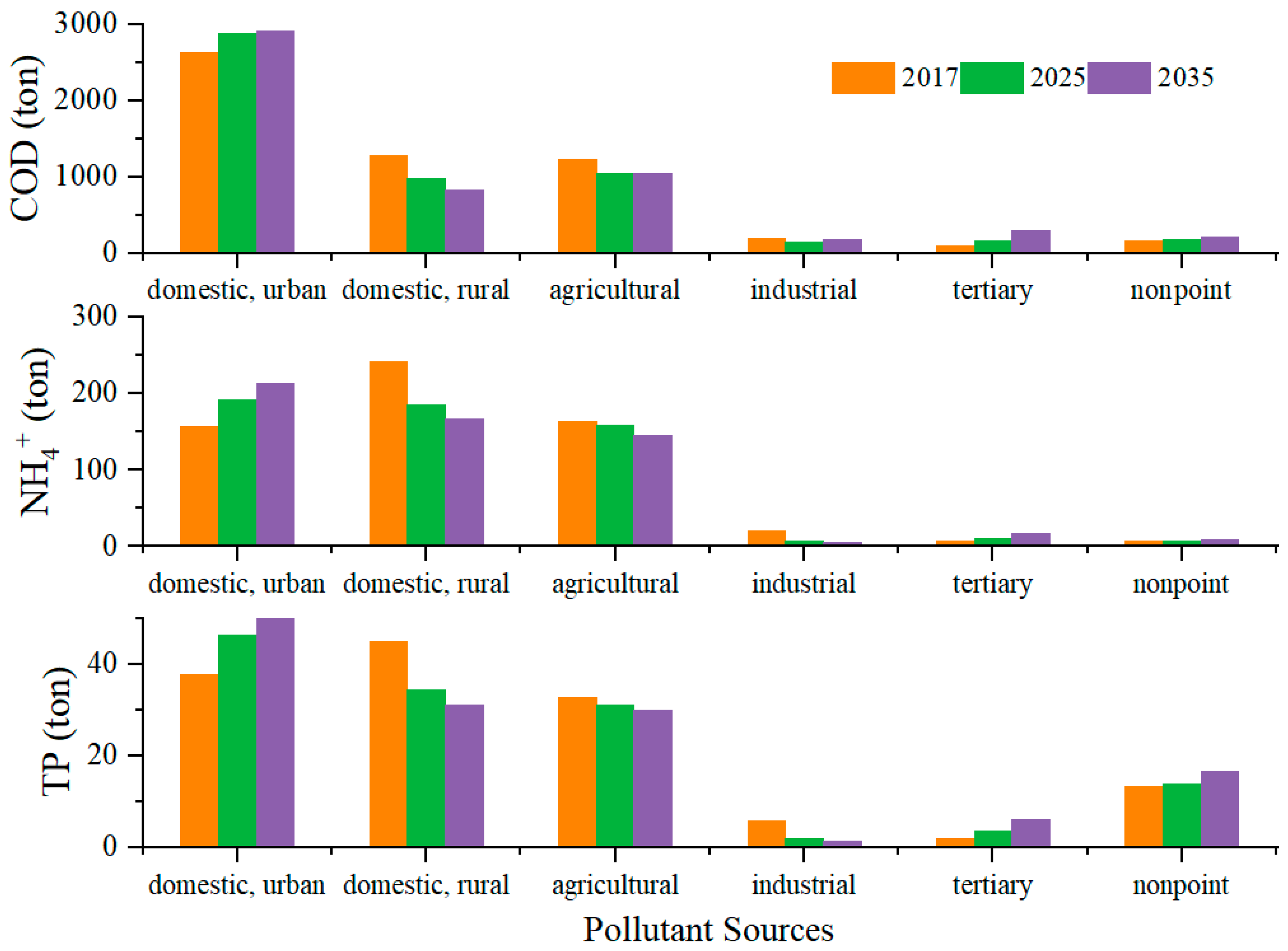
The methodology outlined in Section 3.2 was applied to both estimate the total loads of pollutants and map the spatial distribution of their discharge using the grid scale described in three stages—2017, 2025, and 2035—according to the regional environmental quality statistical yearbooks and the second national survey of pollution sources. Our calculation results of the status quo based on the reference year 2017 showed that pollutant loads will not significantly decrease in the future. In particular, in 2017, COD, NH4+, and TP discharge were 5599.65 tons, 598.82 tons, and 136.86 tons, respectively (Figure 3). In 2025, the COD loads were estimated at 5406.07 tons and 5479.07 tons in 2035; the NH4+ loads at 562.65 tons and 556.80 tons in 2035; and the TP loads at 130.73 tons and 135.76 tons in 2035. In terms of pollutant shares, in 2017, the largest source of COD discharge was urban (domestic), accounting for 46.8% of the total discharge, while the largest source for NH4+, and TP was domestic rural (Figure 3), accounting for 40.5% and 32.8% of the total load, respectively. In 2025 and 2035, domestic urban pollution is projected to become the largest source of TP discharge (35.3% and 37.6%, respectively). In 2035, domestic urban pollution is projected to also be the largest source of NH4+ (38.2%).
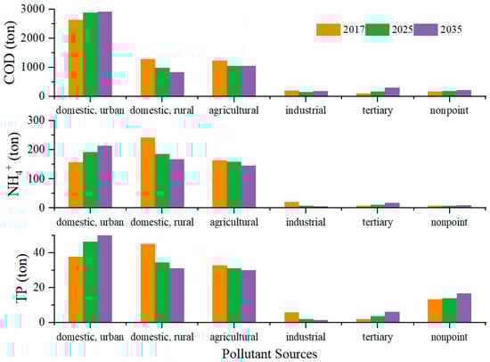
Figure 3.
Pollutant load (ton) by sources.
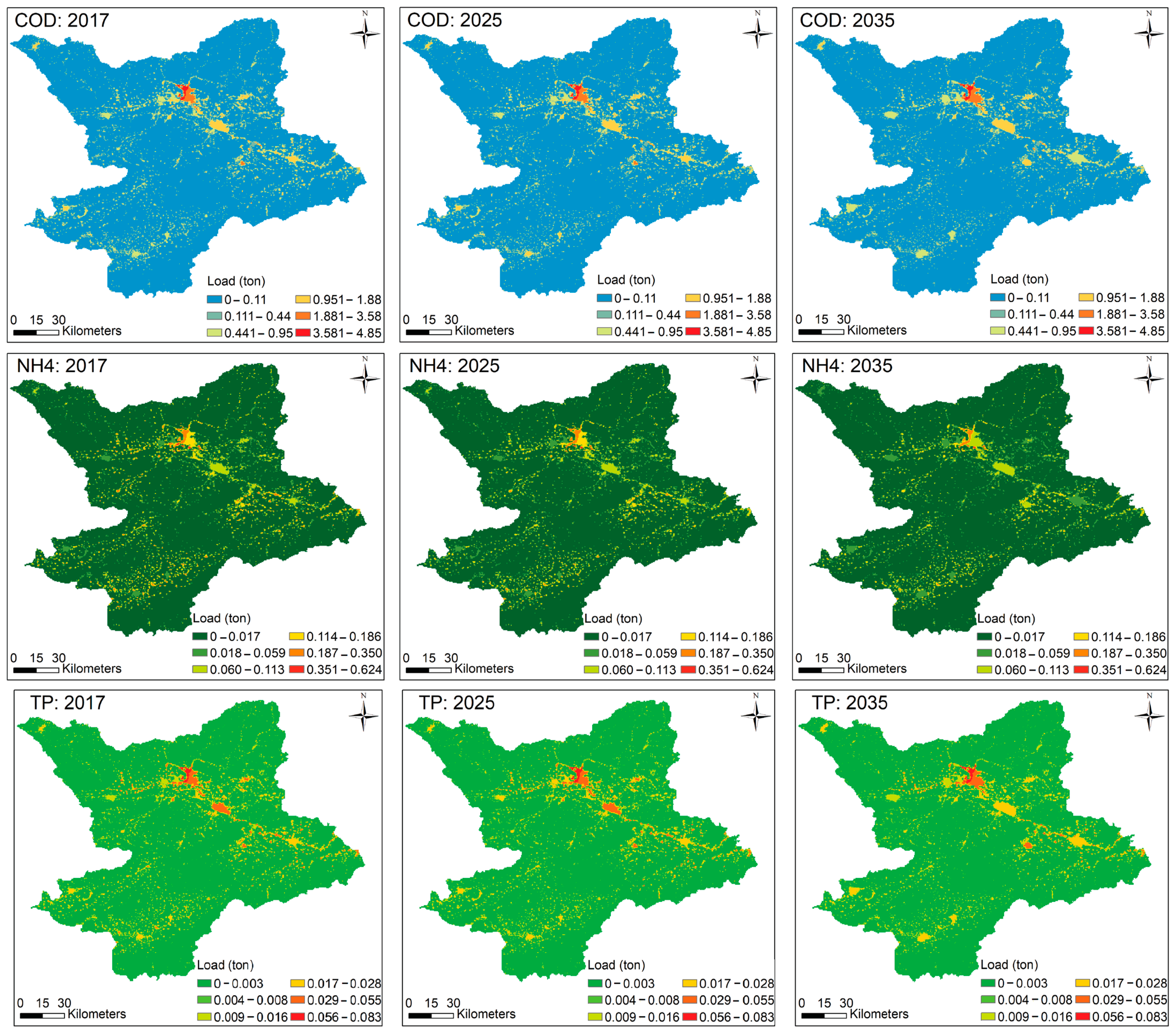
The spatial distribution patterns of COD, NH4+, and TP in 2017, 2025, and 2035 (Figure 4) indicate that urban areas are pollution hotspots, followed by rural areas. This can be attributed mainly to the faster population growth and industrial development rates (Figure S1) outpacing the WWT capacity of the region. This leads to increased pollutant discharges, which, combined with the limited precipitation of this arid area, pose a serious pollution threat to the limited water resources.
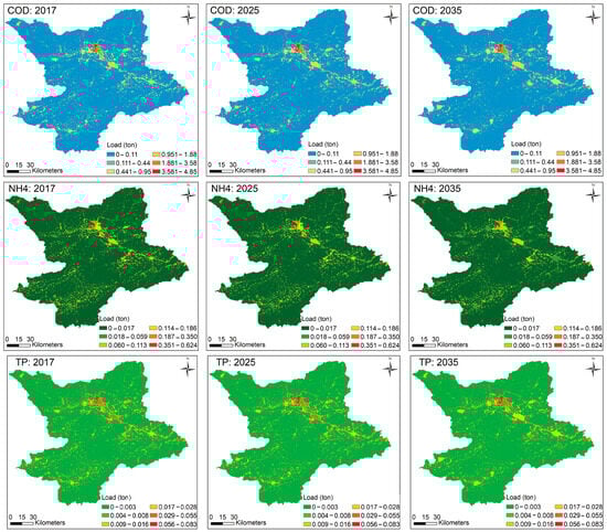
Figure 4.
Spatial distribution of the three major pollutant loads in YRB in 2017, 2025, and 2035.
In 2017, urban areas were responsible for discharges of 5672.81 kg·km−2 of COD, 351.64 kg·km−2 of NH4+, and 108.27 kg·km−2 of TP. The next highest pressure came from rural domestic areas, with discharges of 2516.86 kg·km−2 of COD, 470.98 kg·km−2 of NH4+, and 87.57 kg·km−2 of TP. Agricultural pollution was the third highest, with discharges of 172.70 kg·km−2 of COD, 23.13 kg·km−2 of NH4+, and 4.63 kg·km−2 of TP. By 2035, urban areas are projected to be responsible for discharges of 5380.72 kg·km−2 of COD, 364.84 kg·km−2 of NH4+, and 111.90 kg·km−2 of TP. These are followed by rural areas, with projected discharges of 1758.99 kg·km−2 of COD, 330.94 kg·km−2 of NH4+, and 63.02 kg·km−2 of TP (Figure 4).
Urban areas consistently exhibit the highest COD discharges, though there is a slight decrease from 5672.81 kg·km−2 in 2017 to 5380.72 kg·km−2 in 2035. This trend suggests that while population and industrial growth continue to exert pressure, improvements in WWT might slightly mitigate COD levels. Rural areas also show a decrease in COD discharge from 2516.86 kg·km−2 in 2017 to 1758.99 kg·km−2 in 2035, indicating some effectiveness in addressing domestic pollution. NH4+ discharges show a slight increase in urban areas, from 351.64 kg·km−2 in 2017 to 364.84 kg·km−2 in 2035, highlighting ongoing challenges in treating excessive amounts of nitrogenous waste despite WWT expansion. TP discharges increased slightly in urban areas, from 108.27 kg·km−2 in 2017 to 111.90 kg·km−2 in 2035, indicating persistent issues with phosphorus control, likely from both domestic and industrial sources.
4.3. Changes in the Ecosystem Services
The ecosystem values of Table 1 were applied, as described in Section 3.3, in order to estimate the ES value (ESV) based on the land use maps of the period 2015–2035. The spatial distribution of ESV and its evolution based on the land use changes in the study area are shown in Figure 5. These results illustrate the gradual expansion of the lower ESV due to the expansion of urban land use. At the same time, the high-ESV areas have gradually replaced some areas with lower ESV, reflecting the OPR’s policy outcomes regarding the restoration of the water bodies areas and their protection after 2025.
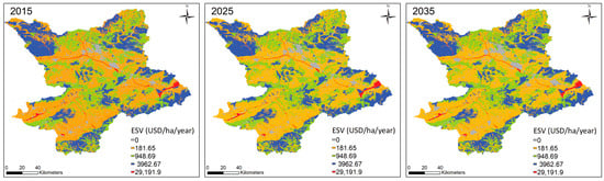
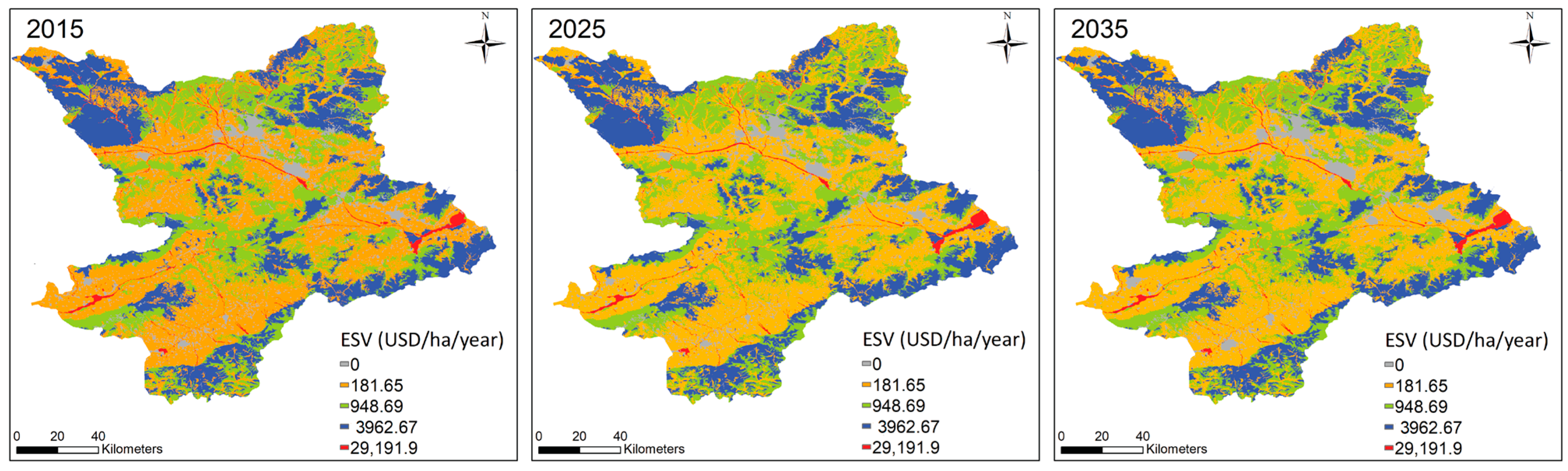
Figure 5.
Spatial distribution of ESV (USD/ha/year) in the period 2015–2035.
To further show the evolution of the ESV, we also present the areas of the different land use types (in km2) based on the ESV coefficients in Table 1 along with their estimated ESV (Table 3). The total estimated ESV in 2015 was USD 3039.16 million. From 2015 to 2025, the ESV of water bodies increased, which is a result of the water bodies restoration according to the OPR policy, as mentioned. From 2025 to 2035, the ESV of farmland, forest, and grassland decreased because these land use types gradually gave way to urban areas. However, the total ESV is projected to be USD 3082.76 million in 2035, which is an increase of USD 43.60 million compared to the 2015 value. Overall, forest land use is the largest contributor to the ESV, with approximately 53.3% of the total ESV, followed by water bodies (28%).
Table 3.
Evolution of the different land use types and ESV (million USD, 2022 values) and the estimated yearly changes in ESV.
5. Discussion
5.1. Land Use Types and Water Quality
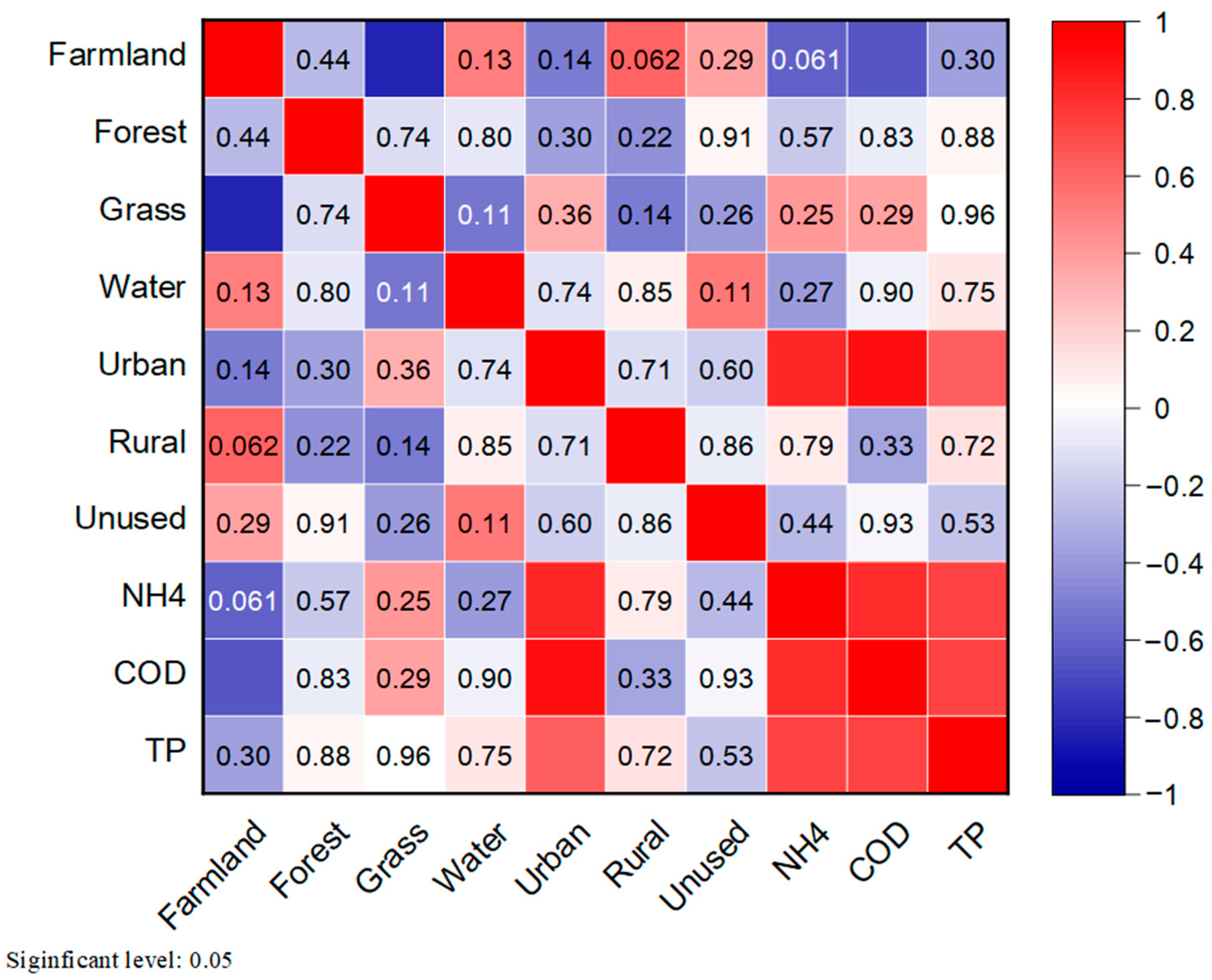
Our study focused mainly on the responses of water pollutant concentrations to land use type changes. To further scrutinize these relationships, we performed a correlation analysis between concentrations of COD, NH4+, and TP at the 10 river water quality sites (Figure 6), collected from the Zhangjiakou Environmental Protection Bureau, and the land use type in each sub-watershed. The results, presented in Figure 6, indicate that, among all the land use types, COD (r = 0.91, p < 0.01), NH4+ (r = 0.84, p < 0.01), and TP (r = 0.63, p < 0.05) concentrations were all significantly correlated with urban areas. This observation confirms that the discharge of urban-related pollutants is a major driver of YRB’s water pollution. As mentioned, urban areas are pollution hotspots due to the high level of discharge following continuous urbanization, as estimated previously (Section 3.2), outpacing the WWTP upgrades in terms of capacity and efficiency.
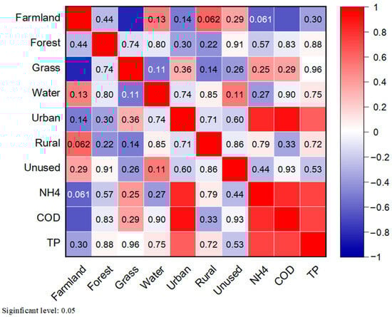
Figure 6.
Correlation analysis for the relationships between river pollutant concentrations and land use types. The concentration data used for the correlation analysis are the long-term mean values of July from the years 2005 to 2019 because July typically experiences the highest precipitation in this region [34,54] and the peak-flow period can provide a stronger correlation between land use and water quality [55]. The value in the panel is the p-value, and the color represents the correlation coefficient.
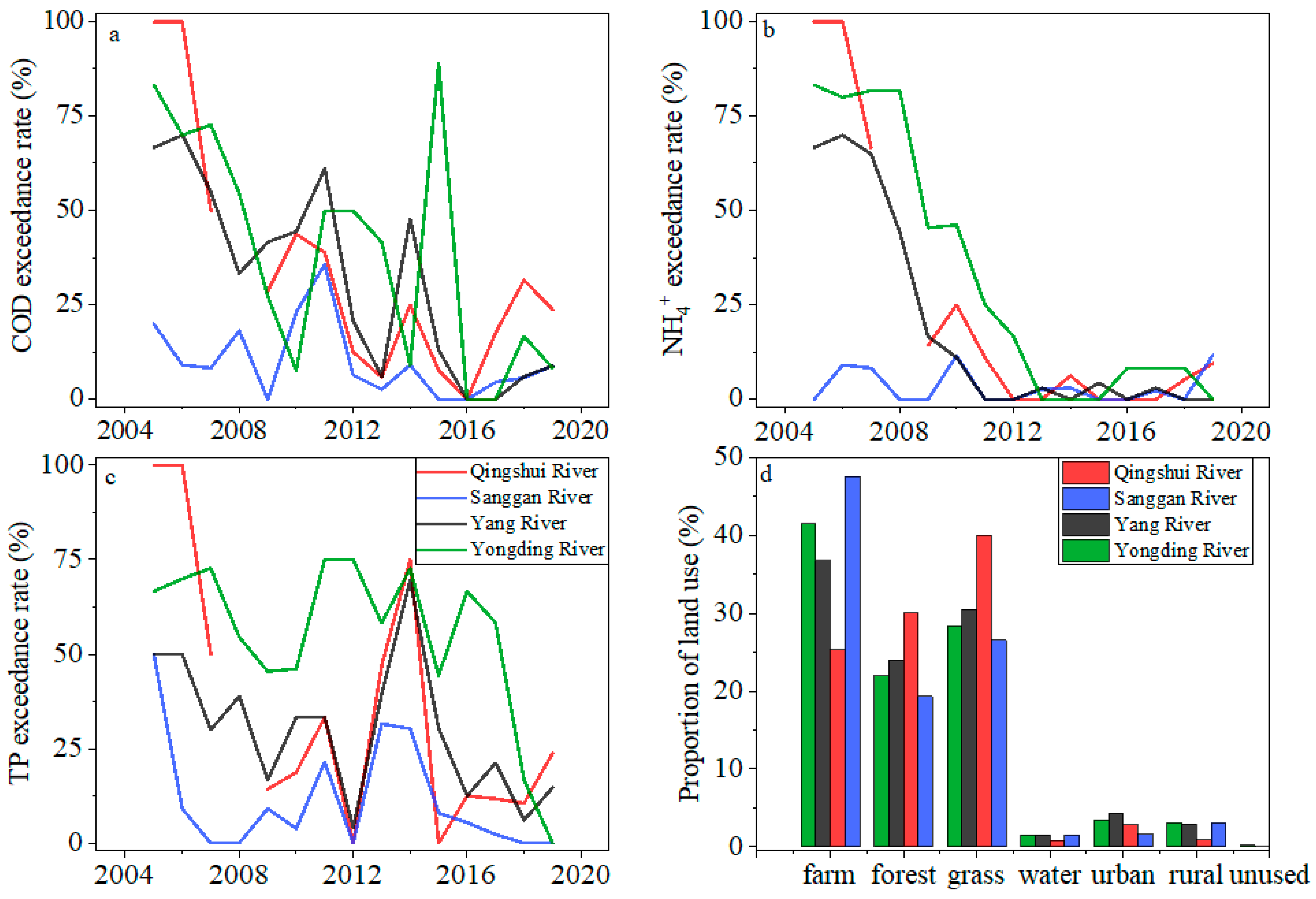
On the river network scale, our results show that changes in water quality trends differed among the rivers (Figure 7). Before 2016, all the rivers experienced poor water quality, and the water quality was highly variable (Figure 7a–c) compared with the concentration targets of Class III of China’s Environmental Quality Standards for Surface Waters [56]. Currently (2017–2019), although the pollutant exceedance rates have significantly decreased, particularly for NH4+ annually, COD and TP still require more attention. It is noted that the exceedance rates of all three pollutants were lowest in the Sanggan River, mainly due to the low percentage of urban land use (low urbanization and population) in the respective watershed (Figure 7d) and the relatively low geographical heterogeneity.
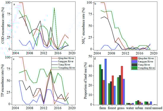
Figure 7.
Annual proportion of the three pollutant concentrations in each river from 2005 to 2019 ((a) COD, (b) NH4+, and (c) TP) exceeding the target concentrations based on China’s Environmental Quality Standards for Surface Waters (Class Ⅲ: COD = 20 mg/L, NH4+ = 1.0 mg/L, and TP = 0.2 mg/L) and the proportion ((d) the land use data were from 2015) of each land use type in the river watershed.
5.2. The Role of Wastewater Treatment
As discussed and indicated already by the results, the two main causes of water pollution in the YRB are high pollutant discharge levels from urban areas due to population and economic growth and decreased natural water flow due to the prevailing arid conditions. This limits the ability of the rivers to dilute water coming from WWTPs, as the rivers in YRB are largely supplied by WWTP effluent [11,57]. The OPR policy is part of broader efforts in China to enhance environmental protection, and already in some areas, the number of WWTPs as well as their efficiency have increased [58,59]. This has been seen so far as the most effective measure to control river pollution, as major pollutants’ concentrations can be significantly reduced from sewage [58,60]. This is also the case in the YRB, where the annual treatment capacity of WWTPs has continued to increase since 2005 [36].
To further study the role of the WWTPs in potential improvements in water quality, we performed a simple linear regression analysis to find relationships between annual water quality. These were based on the major pollutants’ concentrations in the river network from 2005 to 2019, the rates of pollutant concentrations exceeding the target concentrations (exceedance rates), and the annual municipal WWT capacities collected from the Environmental Statistical Yearbooks of Zhangjiakou City. The results of these regressions are shown in Figure 8. As expected, both pollutant concentrations and exceedance rates decreased with the increased WWT capacities, confirming the positive contribution of WWTPs to the improved water quality during the study period.
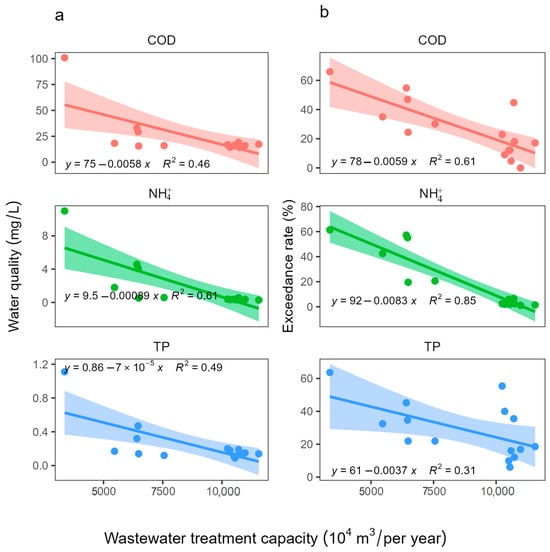
Figure 8.
Linear regression models of annual pollutant concentrations (a) and exceedance rate (b) of the three water quality parameters with WWT capacity (volume of wastewater treated). Different colors represent the pollutants (pink: COD, green: NH4+ and blue: TP), and areas are the 95% confidence interval.
5.3. Improved WWT Efficiency and Spatial Distribution of Pollutants
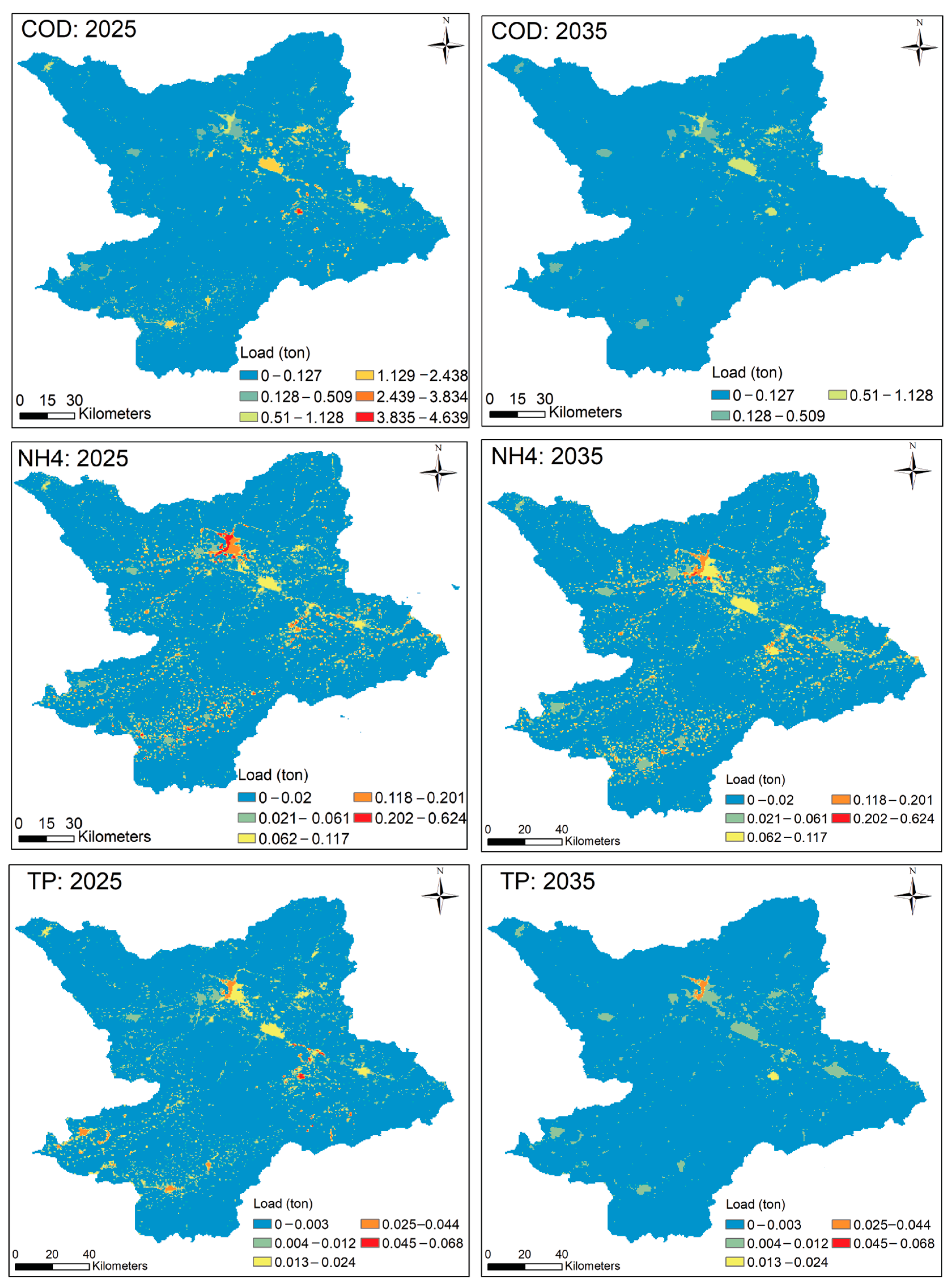
In this section, we present an additional case where the WWTPs expansion follows the OPR-suggested improved efficiencies (Table S2) in the future. This shows the potential improvements in the spatial distribution of the pollutant loads (Figure 9) compared to the results of Figure 4. As expected, it is shown that in 2025 and 2035, the pollutant discharge of each land use type will significantly decrease as a result of the improved treatment efficiency. For example, in 2025, urban discharges of COD will decrease to 4198.62 kg·km−2 and continue to decrease to 2483.37 kg·km−2 in 2035. Considering the limited precipitation, the amount of agricultural non-point source pollution, with little rainfall runoff input, still generates the lowest pollution amounts. These findings are in line with previous research pointing out that urban point sources of nutrients can be the leading cause of surface water quality impairments [61].
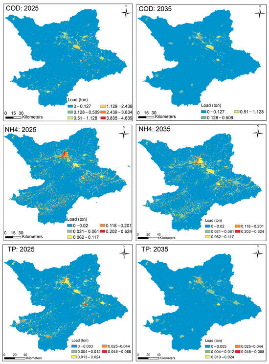
Figure 9.
Spatial distribution of the three major pollutants in the study area in 2025 and 2035, considering improved WWT efficiency.
Given the high pollutant discharge from urban areas and the increased urbanization, the need for efficient wastewater management is vital. In arid and semi-arid areas, like the YRB, where wastewater from domestic (urban and rural) sources is the predominant pollution source and the effluents of WWTPs are often directly discharged into the river network, investing in WWT can make a significant difference (as shown in Figure 9). This observation is also in line with recent research findings highlighting WWTPs’ contribution to China’s water pollution control over the last two decades [59,62].
6. Conclusions
Human-induced land use changes, water use, and water pollution greatly stress water quality and ecosystem degradation, especially in water-scarce regions. Using the YRB in Zhangjiakou City as an example of a typical water-scarce region of North China, we analyzed the impact of land use and WWT on river water quality and ESs. The main pollutants, namely COD, NH4+, and TP, were analyzed. Our results showed that in this semi-arid region, pollutant emissions are highest in densely populated urban areas. Urban areas are the main pollutant sources, with major concentrations found in densely populated cities and towns, followed by rural areas.
Although we quantified and projected the pollutant spatial distribution, this effort for an integrated assessment comes with some unavoidable limitations, which can be improved in future research. The future spatial distribution of pollutants is based on land use changes and the effects of the ORP policy. In reality, pollutant distribution is complex and can be highly variable, and more socioeconomic factors may affect it. Future work should give more attention to the dynamic responses of water quality changes and land use and pollutant control policies at even higher resolution scales.
Nevertheless, this work is a significant first step in connecting land use changes, water pollution, and ESs, as well as their interactions, and this is expected to be an important contribution towards more integrated decision-making, especially for arid developing regions. The spatial pattern of major pollutants and river water quality trends indicate the difficulty in achieving acceptable water quality targets in urban areas without improving the domestic WWT capacity due to the increased population. As mentioned in the discussion section, the expansion and improvement of WWTPs will be key to addressing water pollution. In the YRB, there are ongoing efforts in this direction with the OPR policy. Supporting such policies will be crucial in the future for addressing the potentially increased pollution loads that might occur due to urbanization and industrialization. This paper provides a methodological and analytical approach for integrating spatial assessments of land use changes and ES valuations in water quality. Thus, the contribution of the findings is the ability to target investments in WWTP expansion and improvements in areas that need them most, either in terms of particular land use or ES interest. The OPR and similar policies should be applied in a scientifically supported and transparent way to ensure maximum efficiency and holistic benefits.
Our findings can inform these efforts by targeting areas that pose the greatest pressures in water quality degradation (based on the spatial distribution of pollutant discharges), experience the most intense urbanization rates (based on the land use change maps), or similarly, face significant ES devaluation. The ability to combine and connect these analyses provides valuable information for detecting responses to surface water quality and ESs across different spatiotemporal scales.
Supplementary Materials
The following supporting information can be downloaded at: https://www.mdpi.com/article/10.3390/w16121701/s1, Figure S1: Spatial distribution of the population and GDP of the study area; Table S1: Pollutant production, export loading, and pollutant inflow coefficients in the YRB watershed; Table S2: Pollutant treatment efficiency of different wastewaters in the YRB watershed in three stages. References [18,63,64] were cited in the Supplementary Materials.
Author Contributions
Conceptualization, D.D. and A.A.; methodology, D.D.; software, D.D.; data curation, D.D.; writing—original draft preparation, D.D.; writing—review and editing, A.A. All authors have read and agreed to the published version of the manuscript.
Funding
This research received no external funding.
Data Availability Statement
Data will be made available on request.
Conflicts of Interest
The authors declare no conflicts of interest.
References
- Schandl, H.; Hatfield-Dodds, S.; Wiedmann, T.; Geschke, A.; Cai, Y.; West, J.; Newth, D.; Baynes, T.; Lenzen, M.; Owen, A. Decoupling global environmental pressure and economic growth: Scenarios for energy use, materials use and carbon emissions. J. Clean. Prod. 2016, 132, 45–56. [Google Scholar] [CrossRef]
- Guan, D.; Hubacek, K.; Tillotson, M.; Zhao, H.; Liu, W.; Liu, Z.; Liang, S. Lifting China’s water spell. Environ. Sci. Technol. 2014, 48, 11048–11056. [Google Scholar] [CrossRef] [PubMed]
- Huang, J.; Zhang, Y.; Bing, H.; Peng, J.; Dong, F.; Gao, J.; Arhonditsis, G.B. Characterizing the river water quality in China: Recent progress and on-going challenges. Water Res. 2021, 201, 117309. [Google Scholar] [CrossRef] [PubMed]
- Ma, T.; Sun, S.; Fu, G.; Hall, J.W.; Ni, Y.; He, L.; Yi, J.; Zhao, N.; Du, Y.; Pei, T. Pollution exacerbates China’s water scarcity and its regional inequality. Nat. Commun. 2020, 11, 1–9. [Google Scholar] [CrossRef]
- Sun, S.; Zhou, X.; Liu, H.; Jiang, Y.; Zhou, H.; Zhang, C.; Fu, G. Unraveling the effect of inter-basin water transfer on reducing water scarcity and its inequality in China. Water Res. 2021, 194, 116931. [Google Scholar] [CrossRef] [PubMed]
- Mishra, A.; Alnahit, A.; Campbell, B. Impact of land uses, drought, flood, wildfire, and cascading events on water quality and microbial communities: A review and analysis. J. Hydrol. 2020, 596, 125707. [Google Scholar] [CrossRef]
- Salerno, F.; Gaetano, V.; Gianni, T. Urbanization and climate change impacts on surface water quality: Enhancing the resilience by reducing impervious surfaces. Water Res. 2018, 144, 491–502. [Google Scholar] [CrossRef] [PubMed]
- Tong, S.T.Y.; Chen, W. Modeling the relationship between land use and surface water quality. J. Environ. Manag. 2002, 66, 377–393. [Google Scholar] [CrossRef] [PubMed]
- Fu, B.; Zhang, L.; Xu, Z.; Zhao, Y.; Wei, Y.; Skinner, D. Ecosystem services in changing land use. J. Soils Sediments 2015, 15, 833–843. [Google Scholar] [CrossRef]
- Alamanos, A. Exploring the impact of future land uses on flood risks and ecosystem services, with limited data: Coupling a cellular automata markov (CAM) model, with hydraulic and spatial valuation models. Qeios 2024, 1–25. [Google Scholar] [CrossRef]
- Bussi, G.; Janes, V.; Whitehead, P.G.; Dadson, S.J.; Holman, I.P. Dynamic response of land use and river nutrient concentration to long-term climatic changes. Sci. Total Environ. 2017, 590–591, 818–831. [Google Scholar] [CrossRef]
- Tolessa, T.; Senbeta, F.; Kidane, M. The impact of land use/land cover change on ecosystem services in the central highlands of Ethiopia. Ecosyst. Serv. 2017, 23, 47–54. [Google Scholar] [CrossRef]
- Dupas, R.; Casquin, A.; Durand, P.; Viaud, V. Landscape spatial configuration influences phosphorus but not nitrate concentrations in agricultural headwater catchments. Hydrol. Process. 2023, 37, e14816. [Google Scholar] [CrossRef]
- Salem, A.; Abduljaleel, Y.; Dezső, J.; Lóczy, D. Integrated assessment of the impact of land use changes on groundwater recharge and groundwater level in the Drava floodplain, Hungary. Sci. Rep. 2023, 13, 5061. [Google Scholar] [CrossRef]
- Blyth, E.M.; Arora, V.K.; Clark, D.B.; Dadson, S.J.; De Kauwe, M.G.; Lawrence, D.M.; Melton, J.R.; Pongratz, J.; Turton, R.H.; Yoshimura, K.; et al. Advances in land surface modelling. Curr. Clim. Chang. Rep. 2021, 7, 45–71. [Google Scholar] [CrossRef]
- Subedi, P.; Subedi, K.; Thapa, B. Application of a Hybrid Cellular Automaton–Markov (CA-Markov) Model in Land-Use Change Prediction: A Case Study of Saddle Creek Drainage Basin, Florida. AEES 2013, 1, 126–132. [Google Scholar] [CrossRef]
- Fu, X.; Wang, X.; Yang, Y.J. Deriving suitability factors for CA-Markov land use simulation model based on local historical data. J. Environ. Manag. 2018, 206, 10–19. [Google Scholar] [CrossRef]
- Zhou, X.-Y.; Lei, K.; Meng, W.; Khu, S.-T.; Zhao, J.; Wang, M.; Yang, J. Space–time approach to water environment carrying capacity calculation. J. Clean. Prod. 2017, 149, 302–312. [Google Scholar] [CrossRef]
- Van Meter, K.J.; Basu, N.B. Catchment legacies and time lags: A parsimonious watershed model to predict the effects of legacy storage on nitrogen export. PLoS ONE 2015, 10, e0125971. [Google Scholar] [CrossRef]
- Winkler, K.; Fuchs, R.; Rounsevell, M.; Herold, M. Global land use changes are four times greater than previously estimated. Nat. Commun. 2021, 12, 2501. [Google Scholar] [CrossRef]
- Hasan, S.S.; Zhen, L.; Miah, M.G.; Ahamed, T.; Samie, A. Impact of land use change on ecosystem services: A review. Environ. Dev. 2020, 34, 100527. [Google Scholar] [CrossRef]
- McGrane, S.J. Impacts of urbanisation on hydrological and water quality dynamics, and urban water management: A review. Hydrol. Sci. J. 2016, 61, 2295–2311. [Google Scholar] [CrossRef]
- Singh, S.; Bhardwaj, A.; Verma, V.K. Remote sensing and GIS based analysis of temporal land use/land cover and water quality changes in Harike wetland ecosystem, Punjab, India. J. Environ. Manag. 2020, 262, 110355. [Google Scholar] [CrossRef]
- Monaghan, R.M.; Wilcock, R.J.; Smith, L.C.; Tikkisetty, B.; Thorrold, B.S.; Costall, D. Linkages between land management activities and water quality in an intensively farmed catchment in southern New Zealand. Agric. Ecosyst. Environ. 2007, 118, 211–222. [Google Scholar] [CrossRef]
- Troy, A.; Wilson, M.A. Mapping ecosystem services: Practical challenges and opportunities in linking GIS and value transfer. Ecol. Econ. 2006, 60, 435–449. [Google Scholar] [CrossRef]
- Lawler, J.J.; Lewis, D.J.; Nelson, E.; Plantinga, A.J.; Polasky, S.; Withey, J.C.; Helmers, D.P.; Martinuzzi, S.; Pennington, D.; Radeloff, V.C. Projected land-use change impacts on ecosystem services in the United States. Proc. Natl. Acad. Sci. USA 2014, 111, 7492–7497. [Google Scholar] [CrossRef]
- Gomes, E.; Inácio, M.; Bogdzevič, K.; Kalinauskas, M.; Karnauskaitė, D.; Pereira, P. Future land-use changes and its impacts on terrestrial ecosystem services: A review. Sci. Total Environ. 2021, 781, 146716. [Google Scholar] [CrossRef] [PubMed]
- Xue, M.; Luo, Y. Dynamic variations in ecosystem service value and sustainability of urban system: A case study for Tianjin city, China. Cities 2015, 46, 85–93. [Google Scholar] [CrossRef]
- Koundouri, P.; Boulton, A.J.; Datry, T.; Souliotis, I. Ecosystem services, values, and societal perceptions of intermittent rivers and ephemeral streams. In Intermittent Rivers and Ephemeral Streams; Elsevier: Amsterdam, The Netherlands, 2017; pp. 455–476. ISBN 9780128038352. [Google Scholar]
- Alamanos, A.; Brouwer, R. The cost-effectiveness of wetlands as a nature-based solution to reduce phosphorous runoff. In Proceedings of the International Association for Great Lakes Research (IAGLR) Conference, Virtual, 9–11 June 2020. [Google Scholar]
- Garcia, J.A.; Alamanos, A. Integrated Modelling Approaches for Sustainable Agri-Economic Growth and Environmental Improvement: Examples from Greece, Canada and Ireland. Land 2022, 11, 1548. [Google Scholar] [CrossRef]
- Wang, S.; Li, K.; Liang, S.; Zhang, P.; Lin, G.; Wang, X. An integrated method for the control factor identification of resources and environmental carrying capacity in coastal zones: A case study in Qingdao, China. Ocean. Coast. Manag. 2017, 142, 90–97. [Google Scholar] [CrossRef]
- Fang, C.; Cui, X.; Li, G.; Bao, C.; Wang, Z.; Ma, H.; Sun, S.; Liu, H.; Luo, K.; Ren, Y. Modeling regional sustainable development scenarios using the Urbanization and Eco-environment Coupler: Case study of Beijing-Tianjin-Hebei urban agglomeration, China. Sci. Total Environ. 2019, 689, 820–830. [Google Scholar] [CrossRef]
- Du, Y.; Bao, A.; Zhang, T.; Ding, W. Quantifying the impacts of climate change and human activities on seasonal runoff in the Yongding River basin. Ecol. Indic. 2023, 154, 110839. [Google Scholar] [CrossRef]
- Falkenmark, M. The massive water scarcity now threatening Africa: Why isn’t it being addressed? Ambio 1989, 18, 112–118. [Google Scholar]
- Dai, D.; Lei, K.; Wang, R.; Lv, X.; Hu, J.; Sun, M. Evaluation of river restoration efforts and a sharp decrease in surface runoff for water quality improvement in North China. Environ. Res. Lett. 2022, 17, 044028. [Google Scholar] [CrossRef]
- Jiang, B.; Wong, C.P.; Lu, F.; Ouyang, Z.; Wang, Y. Drivers of drying on the Yongding River in Beijing. J. Hydrol. 2014, 519, 69–79. [Google Scholar] [CrossRef]
- Dai, D.; Sun, M.; Lv, X.; Hu, J.; Zhang, H.; Xu, X.; Lei, K. Comprehensive assessment of the water environment carrying capacity based on the spatial system dynamics model, a case study of Yongding River Basin in North China. J. Clean. Prod. 2022, 344, 131137. [Google Scholar] [CrossRef]
- Dai, D.; Xu, X.; Sun, M.; Hao, C.; Lv, X.; Lei, K. Decrease of both river flow and quality aggravates water crisis in North China: A typical example of the upper Yongding River watershed. Environ. Monit. Assess. 2020, 192, 421. [Google Scholar] [CrossRef] [PubMed]
- Yu, Y.; Ma, M.; Zheng, F.; Liu, L.; Zhao, N.; Li, X.; Yang, Y.; Guo, J. Spatio-Temporal Variation and Controlling Factors of Water Quality in Yongding River Replenished by Reclaimed Water in Beijing, North China. Water 2017, 9, 453. [Google Scholar] [CrossRef]
- Lei, W.; Wang, Z.J.; Koike, T.; Hang, Y.; Yang, D.W.; Shan, H. The assessment of surface water resources for the semi-arid Yongding River Basin from 1956 to 2000 and the impact of land use change. Hydrol. Process. 2010, 24, 1123–1132. [Google Scholar]
- Hou, L.; Peng, W.; Qu, X.; Chen, Q.; Fu, Y.; Dong, F.; Zhang, H. Runoff changes based on dual factors in the upstream area of Yongding River basin. Pol. J. Environ. Stud. 2019, 28, 143. [Google Scholar] [CrossRef]
- Clark Labs IDRISISelva 17. Available online: https://clarklabs.org/download/idrisi-selva-service-update-to-17-2/ (accessed on 22 May 2024).
- Rahman, M.M.; Szabó, G. Multi-objective urban land use optimization using spatial data: A systematic review. Sustain. Cities Soc. 2021, 74, 103214. [Google Scholar] [CrossRef]
- Costanza, R.; d’Arge, R.; Groot, R.; Farber, S.; Grasso, M.; Hannon, B.; Limburg, K.; Naeem, S.; O’Neill, R.V.; Paruelo, J.; et al. The value of the world’s ecosystem services and natural capital. Nature 1997, 387, 253–260. [Google Scholar] [CrossRef]
- Pascual, U.; Balvanera, P.; Anderson, C.B.; Chaplin-Kramer, R.; Christie, M.; González-Jiménez, D.; Martin, A.; Raymond, C.M.; Termansen, M.; Vatn, A.; et al. Diverse values of nature for sustainability. Nature 2023, 620, 813–823. [Google Scholar] [CrossRef] [PubMed]
- de Groot, R.S.; Alkemade, R.; Braat, L.; Hein, L.; Willemen, L. Challenges in integrating the concept of ecosystem services and values in landscape planning, management and decision making. Ecol. Complex 2010, 7, 260–272. [Google Scholar] [CrossRef]
- Rahman, M.; Szabó, G. Impact of land use and land cover changes on urban ecosystem service value in dhaka, bangladesh. Land 2021, 10, 793. [Google Scholar] [CrossRef]
- National Development and Reform Commission, Overall Plan of Comprehensive Management and Ecological Restoration of Yongding River. Available online: https://www.ndrc.gov.cn/xxgk/jianyitianfuwen/qgrddbjyfwgk/202107/t20210708_1288136.html (accessed on 22 May 2024).
- Eastman, J.R. IDRISI Selva Manual; Clark Labs-Clark University: Worcester, MA, USA, 2012. [Google Scholar]
- Kityuttachai, K.; Tripathi, N.; Tipdecho, T.; Shrestha, R. CA-Markov analysis of constrained coastal urban growth modeling: Hua Hin seaside city, Thailand. Sustainability 2013, 5, 1480–1500. [Google Scholar] [CrossRef]
- Zhai, L.; Cheng, S.; Sang, H.; Xie, W.; Gan, L.; Wang, T. Remote sensing evaluation of ecological restoration engineering effect: A case study of the Yongding River Watershed, China. Ecol. Eng. 2022, 182, 106724. [Google Scholar] [CrossRef]
- Beijing Water Authority. Green Yongding River: The Construction Plan for an Ecological Corridor; Beijing Water Authority: Beijing, China, 2009. (In Chinese)
- Pernet-Coudrier, B.; Qi, W.; Liu, H.; Müller, B.; Berg, M. Sources and pathways of nutrients in the semi-arid region of Beijing-Tianjin, China. Environ. Sci. Technol. 2012, 46, 5294–5301. [Google Scholar] [CrossRef] [PubMed]
- Dupas, R.; Musolff, A.; Jawitz, J.W.; Rao, P.S.C.; Jäger, C.G.; Fleckenstein, J.H.; Rode, M.; Borchardt, D. Carbon and nutrient export regimes from headwater catchments to downstream reaches. Biogeosciences 2017, 14, 4391–4407. [Google Scholar] [CrossRef]
- GB 3838-2002; Environmental Quality Standards for Surface Water. Ministry of Ecological Environment of the People’s Republic of China: Beijing, China, 2002.
- Cheng, P.; Li, X.; Su, J.; Hao, S. Recent water quality trends in a typical semi-arid river with a sharp decrease in streamflow and construction of sewage treatment plants. Environ. Res. Lett. 2018, 13, 014026. [Google Scholar] [CrossRef]
- Zhang, Q.H.; Yang, W.N.; Ngo, H.H.; Guo, W.S.; Jin, P.K.; Dzakpasu, M.; Yang, S.J.; Wang, Q.; Wang, X.C.; Ao, D. Current status of urban wastewater treatment plants in China. Environ. Int. 2016, 92–93, 11–22. [Google Scholar] [CrossRef] [PubMed]
- Tang, W.; Pei, Y.; Zheng, H.; Zhao, Y.; Shu, L.; Zhang, H. Twenty years of China’s water pollution control: Experiences and challenges. Chemosphere 2022, 295, 133875. [Google Scholar] [CrossRef] [PubMed]
- Huang, J.; Zhang, Y.; Arhonditsis, G.B.; Gao, J.; Chen, Q.; Wu, N.; Dong, F.; Shi, W. How successful are the restoration efforts of China’s lakes and reservoirs? Environ. Int. 2019, 123, 96–103. [Google Scholar] [CrossRef] [PubMed]
- Jenny, J.-P.; Normandeau, A.; Francus, P.; Taranu, Z.E.; Gregory-Eaves, I.; Lapointe, F.; Jautzy, J.; Ojala, A.E.K.; Dorioz, J.-M.; Schimmelmann, A.; et al. Urban point sources of nutrients were the leading cause for the historical spread of hypoxia across European lakes. Proc. Natl. Acad. Sci. USA 2016, 113, 12655–12660. [Google Scholar] [CrossRef]
- Tong, Y.; Wang, M.; Peñuelas, J.; Liu, X.; Paerl, H.W.; Elser, J.J.; Sardans, J.; Couture, R.-M.; Larssen, T.; Hu, H.; et al. Improvement in municipal wastewater treatment alters lake nitrogen to phosphorus ratios in populated regions. Proc. Natl. Acad. Sci. USA 2020, 117, 11566–11572. [Google Scholar] [CrossRef]
- Cheng, P. Study of Typical River Water Quality Target Management Technique in the North China; Research Center for Eco-Environmental Sciences Chinese Academy of Sciences: Beijing, China, 2018; p. 148. [Google Scholar]
- Zhu, M. Study on Agricultural NPS Loads of Haihe Basin and Assessment on its Environmental Impact; Chinese Academy of Agricultural Sciences: Beijing, China, 2011. [Google Scholar]


Disclaimer/Publisher’s Note: The statements, opinions and data contained in all publications are solely those of the individual author(s) and contributor(s) and not of MDPI and/or the editor(s). MDPI and/or the editor(s) disclaim responsibility for any injury to people or property resulting from any ideas, methods, instructions or products referred to in the content. |
© 2024 by the authors. Licensee MDPI, Basel, Switzerland. This article is an open access article distributed under the terms and conditions of the Creative Commons Attribution (CC BY) license (https://creativecommons.org/licenses/by/4.0/).