A New Numerical Method to Evaluate the Stability of Dike Slope Considering the Influence of Backward Erosion Piping

Abstract

Backward erosion piping, a soil erosion phenomenon induced by seepage, compromises the stability of water-retaining structures such as dikes. During floods, the seepage in the dike body increases due to high water levels, which directly affects the progression of the piping channel. The formation of the piping channel then impacts the stability of the dike. In this paper, an improved piping model that considers the impact of seepage in the dike body is proposed based on Wewer’s model. Specifically, we added a seepage field of the dike body to the original model to account for the impact of dike-body seepage on the evolution of piping. The seepage field of the dike body is solved using Darcy’s law and the continuity equation for unsaturated porous media. In addition, this approach also incorporates the coupling effect of seepage stress. The accuracy of the model was verified through comparing the calculated results with the IJkdijk experiment and Wewer’s results. The effects of BEP on dike stability were investigated using the proposed improved piping model. The two major conclusions of the study are that (1) the incorporation of unsaturated seepage enhanced the performance of the piping model, allowing it to more accurately simulate the development of pipe length and the changing of pore pressure; and (2) the formation of the pipe impacted dike stability, leading to a substantial reduction in the safety factor of the dike slope.

1. Introduction

Backward erosion piping (BEP) is a prevalent natural disaster that significantly compromises the stability of dikes, often resulting in catastrophic events like dike failures, and exerting a substantial impact on the surrounding areas. BEP generally refers to the contact erosion between different soil layers under the action of seepage. Fine particles are carried by pore water to flow in the soil “pipe” and gush out at the pipe outlet [1]. To study the impact of piping on dike stability, the key lies in the simulation of the piping phenomenon. Scholars have studied BEP through both theoretical and experimental approaches [2,3,4,5,6,7,8,9]. These studies have revealed the critical conditions for piping initiation and the influencing factors of piping. However, these studies were limited by theoretical assumptions and experimental scale, and thus had certain limitations. Some scholars have used numerical simulations to study piping issues [10,11,12,13,14,15,16]. These numerical piping models can be categorized into four groups. The first group of models is based on the discrete element method (DEM) [17,18,19,20,21]. These models can simulate particle interaction, enabling microscopic-level simulation of piping phenomena. The second group of models consider soil as a porous medium composed of a soil skeleton, fine particles, and pore water [22]. In these models, the internal erosion process is generally simulated by establishing coupled mechanical equations for groundwater flow, fine particle movement, and soil-skeleton deformation. The models in the third group define the flow in the piping zone by coupling seepage and pipe flow [23,24]. In the model, Darcy’s law is used to simulate seepage in the soil zone, and pipeline flow theory is used to simulate flow in the pipeline zone. The head and discharge on the common boundary of the two regions are equal. The fourth group of models depict the piping zone as a porous medium with extremely high permeability rather than a fluid-flowing conduit [25,26]. This approach relies on the assumption that the fluid flow within the erosion channel is laminar, a notion supported by experiments [27]. Wewer et al. [28] established a transient BEP model and proved the applicability of the bedload transport equation in piping erosion research based on this approach. Specifically, the seepage field of the dike foundation is solved using Darcy’s law and the continuity equation, and the erosion of piping is calculated by the laminar bedload transport equation and Exner sediment mass conservation equation. The transient BEP model not only predicts the temporal evolution of erosion channels but also detects changes in pore pressure caused by piping. However, it solely simulates the seepage field of the dike foundation, overlooking the impact of dike-body seepage and seepage–stress coupling.

Research methods for slope stability include traditional methods such as the limit equilibrium method [29,30,31] and the finite element method [32,33]. These traditional methods are already well-developed and mature. Additionally, in recent years, new methods based on neural network prediction for slope stability have been proposed [34]. These methods have extensive application value and prospects.

It is evident that there are extensive results in both BEP and slope instability research, but they are rarely analyzed concurrently despite the fact that BEP may likely impact the dike stability of the slope. Some experimental and numerical studies have only investigated the “causal effects” between BEP and slope stability [35,36,37]. Rahimi [38] proposed a performance model that couples slope instability with BEP, simulating the impact of BEP on dike slope stability. This model simulates BEP by controlling the hydraulic conductivity of piping zones and stability assessment using the strength-reduction method. Rahimi’s research revealed the impact of BEP on dike stability and conducted a quantitative analysis. However, the treatment of the piping evolution was relatively simple, and the study did not provide changes in pore pressure during the piping-evolution process.

In summary, although many achievements have been made in the research on BEP and slope stability, studies on these two aspects have been relatively independent and rarely analyzed concurrently. There is also limited research on the impact of piping on dike slope stability. In this paper, an improved BEP model considering the influence of unsaturated seepage in the dike body and seepage stress coupling on piping development is proposed based on Wewer’s transient BEP model. And based on this improved model, the paper investigates the effects of piping development on dike seepage, deformation, and stability. This model is based on the assumption that laminar flow is always present inside the pipe during the piping process [27]. The main objective of this study was to simulate the evolution of piping channels more accurately using an improved BEP model, and to investigate the impact of the formation of backward erosion piping channels on dike stability. The following is the main framework of this paper:

• A brief description of Wewer’s BEP model;
• Improvement of Wewer’s BEP model;
• Verification of the improved piping model;
• Simulation and analysis of piping erosion using the improved piping model.

2. Wewer’s BEP Model Based on Porous Media Seepage

In Wewer’s BEP model [28], the continuity equation of fluid is used to solve the groundwater flow. The erosion criterion is established to judge the occurrence of piping. The erosion rate is calculated based on the bedload transport equation and Exner mass conservation equation, and then the pipe length is calculated.

Based on porous media seepage, Wewer et al. established a BEP model (hereafter referred to as the W-model). In this model, groundwater flow in the porous media is simulated using Darcy’s law combined with the equation of fluid continuity:

$${\rho }_{\mathrm{f}}S\frac{\partial p}{\partial t}+\nabla \cdot \left({\rho }_{\mathrm{f}}{\mathit{u}}_{\mathrm{f}}\right)=0$$

(1)

where ${\rho }_{\mathrm{f}}$ represents the fluid density, $S$ is the storage, $p$ is the pore pressure, and ${\mathit{u}}_{\mathrm{f}}$ is the seepage velocity.

The occurrence of piping is determined by defining the critical conditions for incipient particle motion. A dimensionless Shields parameter in sediment transport is developed as a threshold erosion criterion for initial particle motion:

$$\theta =\frac{{\tau }_w}{\left({\rho }_p-{\rho }_f\right)gd}$$

(2)

where ${\rho }_p$ is the particle density, $d$ is the characteristic particle size, and ${\tau }_w$ denotes the particle driving force (wall shear stress),

$${\tau }_w=\frac{1}{2}\frac{\partial p}{\partial x}h$$

(3)

where $\partial p/\partial x$ is the local pressure gradient in the horizontal direction and $h$ represents the pipe height.

Based on van Beek’s laminar flow assumption [27], the erosion rate of piping can be calculated using the bedload transport equations and the Exner mass conservation equation, i.e.,

$$q_b=q_b^{*}d\sqrt{\frac{\left({\rho }_p-{\rho }_f\right)}{{\rho }_f}gd}$$

(4)

and

$$\frac{\delta A}{\delta t}=\frac{1}{1-n}{q}_{\mathrm{b}}$$

(5)

where $A$ is the erosion area, $n$ is the porosity, $q_{\mathrm{b}}$ is the bedload transport rate, and $q_{\mathrm{b}}^{*}$ is the dimensionless bedload transport rate.

Based on the research of Van Esch [39] that pipe height is described as a function of the particle diameter, Wewer established a relationship between the pipe height $l$ and length $h$:

$$h\left(l\right)=10d\sqrt{\frac{l}{l_{\max }}}$$

(6)

where $l_{\max }$ is maximum pipe length. Then, the length of the erosion channel can be determined through geometric relationships and Equation (6):

$$l={\left(\frac{A\sqrt{l_{\max }}}{10d}\right)}^{\frac{2}{3}}$$

(7)

3. An Improved Piping Model Considering Unsaturated Seepage in the Dike Body and Seepage–Stress Coupling

Based on the BEP model, Wewer tested four different empirical transport formulas $q_{\mathrm{b}}^{*}$, proving the applicability of bedload transport equations in piping simulation. The model not only predicts the pipe progression in time, it also allows for an identification of pore pressure transitions due to the erosion process. But the model has its inadequacy, as it does not consider the seepage of the dike body. BEP occurs at the interface between the foundation and the dike body [40]. The development of piping is not only dependent on the seepage of the foundation, but is also influenced by the seepage of the dike body. However, the model only simulates the seepage field of the foundation, ignoring the influence of dike-body seepage on the evolution of piping. Therefore, based on the theory of unsaturated seepage, this paper proposes an improved BEP model while considering the seepage of the dike body. The simulated results are closer to the experimental results than Wewer’s results were. Moreover, the improved model also accounts for the coupling effect of seepage stress, which can simulate the deformation and stability changes of the dike during the piping process.

3.1. The Governing Equations for Unsaturated Flow in Porous Media

Generally, the upper part of the dike body is in an unsaturated state, while the area below the infiltrated surface is saturated. For such problems, the fluid continuity equation in unsaturated porous media is required. In cases of time-dependent problems, the equation of fluid continuity is expressed as

$${\rho }_f\left(S_{\mathrm{e}}{S}_{\mathrm{p}}+\frac{C_{\mathrm{m}}}{{\rho }_{\mathrm{f}}\mathrm{g}}\right)\frac{\partial p}{\partial t}+\nabla \cdot \left({\rho }_{\mathrm{f}}{\mathit{u}}_{\mathrm{f}}\right)=0$$

(8)

where $S_{\mathrm{e}}$ is the saturation, $p$ is the pore pressure, $C_{\mathrm{m}}$ is the specific water capacity, ${\rho }_{\mathrm{f}}$ is the fluid density, $\mathrm{g}$ is the gravitational acceleration, ${\mathit{u}}_{\mathrm{f}}$ is the seepage velocity, and $S_{\mathrm{p}}$ is the storage. The storage capacity of the aquifer itself depends on soil porosity, compressibility of pore fluids, and compressibility of the soil matrix:

$$S_{\mathrm{p}}=n{\chi }_{\mathrm{f}}+\left(1-n\right){\chi }_{\mathrm{p}}$$

(9)

where ${\chi }_{\mathrm{p}}$ is the compressibility of soil matrix, $n$ is the porosity, and ${\chi }_{\mathrm{f}}$ represents the compressibility of pore fluid.

Groundwater flow in porous media is generally modeled using Darcy’s law, where Darcy velocity ${\mathit{u}}_{\mathrm{f}}$ can be expressed as

$${\mathit{u}}_{\mathrm{f}}=-\frac{\kappa }{\mu }\left({\rho }_{\mathrm{f}}\mathrm{g}\nabla H\right)$$

(10)

where $\kappa$ represents the intrinsic permeability, $\mu$ denotes the dynamic viscosity, $\mathrm{g}$ represents the gravitational acceleration, and $\nabla H$ denotes the hydraulic gradient.

To accurately simulate seepage in unsaturated soil, it is essential to utilize a retention model to depict its water retention characteristics, which helps establish the relationship between permeability, saturation, and pore pressure. In this study, the retention model proposed by Van Genuchten [41] was adopted:

$$\left\{\begin{array}{c}\kappa ={\kappa }_{\mathrm{s}}{\kappa }_{\mathrm{r}}\left(S_{\mathrm{e}}\right)\\ \theta ={\theta }_{\mathrm{r}}+S_{\mathrm{e}}\left({\theta }_{\max }-{\theta }_{\min }\right)\\ C_{\mathrm{m}}=\frac{\partial \theta }{\partial p}=\left({\theta }_{\max }-{\theta }_{\min }\right)\frac{\partial S_{\mathrm{e}}}{\partial p}\end{array}\right.$$

(11)

where ${\kappa }_{\mathrm{s}}$ represents the saturated permeability, ${\kappa }_{\mathrm{r}}$ is the relative permeability, $\theta$ is the volume fraction of the liquid, ${\theta }_{\max }$ is the maximum volume fraction of the liquid, and ${\theta }_{\min }$ denotes the minimum volume fraction of the liquid. The water capacity $C_{\mathrm{m}}$ describes the relationship between $\theta$ and $p$.

The sediment transport rate $q_{\mathrm{b}}$ in Equation (4) is calculated using Yalin’s dimensionless bedload transport rate [42]:

$$q_{\mathrm{b}}^{*}=0.635s\sqrt{\theta }\left[1-\frac{\ln \left(1+\mathrm{as}\right)}{\mathrm{as}}\right]$$

(12)

where $\mathrm{a}$ and $\mathrm{s}$ are the Yalin’s parameters.

3.2. Seepage–Stress Coupling Equation

The advancement of piping can induce alterations in pore pressure, subsequently impacting the stress state of the dike. In the calculation of seepage–stress coupling, the effect of pore water pressure on the stress field can be described by using effective stress in the equilibrium equation. The equilibrium differential equation is given by

$$\rho \frac{{\partial }^2\mathit{u}}{\partial t^2}=\nabla \cdot {\mathit{\sigma }}^{\prime }+{\mathit{F}}_{\mathrm{v}}$$

(13)

where $\mathit{u}$ is the displacement, ${\mathit{F}}_{\mathrm{v}}$ is the body force per volume, and ${\mathit{\sigma }}^{\prime }$ is the effective stress, which is controlled by the pore pressure. The calculation formula is

$${\mathit{\sigma }}^{\prime }=\mathit{\sigma }-{\alpha }_B\left(p-p_{\mathrm{ref}}\right)\mathbf{I}$$

(14)

where $\mathit{\sigma }$ is the total stress, ${\alpha }_B$ is the Biot–Willis coefficient, $p$ is the water pressure, and $p_{\mathrm{ref}}$ is the reference pressure level. The constitutive equation is given by

$$\mathit{\sigma }=\mathit{C}:\left(\mathit{\epsilon }-{\mathit{\epsilon }}_{\mathrm{pl}}\right)$$

(15)

where $\mathit{C}$ is the elastic tensor, $\mathit{\epsilon }$ is the total strain, and ${\mathit{\epsilon }}_{\mathrm{pl}}$ represents the plastic strain. The increment of plastic strain is determined by the plastic potential theory:

$$\mathrm{d}{\mathit{\epsilon }}_{\mathrm{pl}}=\mathrm{\Lambda }\frac{\partial G}{\partial \mathit{\sigma }}$$

(16)

where $\mathrm{\Lambda }$ is the plastic factor, $\partial G/\partial \mathit{\sigma }$ is the direction of plastic-strain flow, $\mathit{\sigma }$ is the stress tensor, and $G$ is the plastic potential function, consistent with the yield surface function in the associated flow.

The yield function adopts the Drucker–Prager criterion:

$$F_{D\_P}=\sqrt{J_2}+\alpha I_1-k$$

(17)

where $J_2$ is the second invariant of deviator component of stress tensor, $I_1$ is the first invariant of stress, and $\alpha$ and $k$ are the material constants, calculated by matching with the Mohr coulomb criterion:

$$\alpha =\frac{\tan \varphi }{\sqrt{9+12{\tan }^2\varphi }},k=\frac{3c}{\sqrt{9+12{\tan }^2\varphi }}$$

(18)

where $c$ is the cohesion and $\varphi$ is the angle of internal friction. The plastic factor is obtained from the consistency condition $\mathrm{\Lambda }{\stackrel{·}{F}}_{D\_P}=0$, and the increment of plastic strain can be determined by Equation (16).

3.3. Stability Analysis

This study employed the strength-reduction method to evaluate the stability of the dike body. Its advantage lies in its capability to offer stress–strain magnitudes, displacement distributions of the soil, rigorous solution processes, and precise results. In the strength-reduction method, the shear-strength index of the soil continually reduces until sliding areas and extensive plastic deformations appear in the dike slope. At this point, the reduction coefficient represents the safety factor of the slope:

$$c_{\mathrm{m}}=c/F$$

(19)

$${\phi }_{\mathrm{m}}=\arctan \left(\tan \phi /F\right)$$

(20)

where $c_{\mathrm{m}}$ is the reduced cohesion, ${\phi }_{\mathrm{m}}$ is the reduced angle of internal friction, and $F$ is the safety factor.

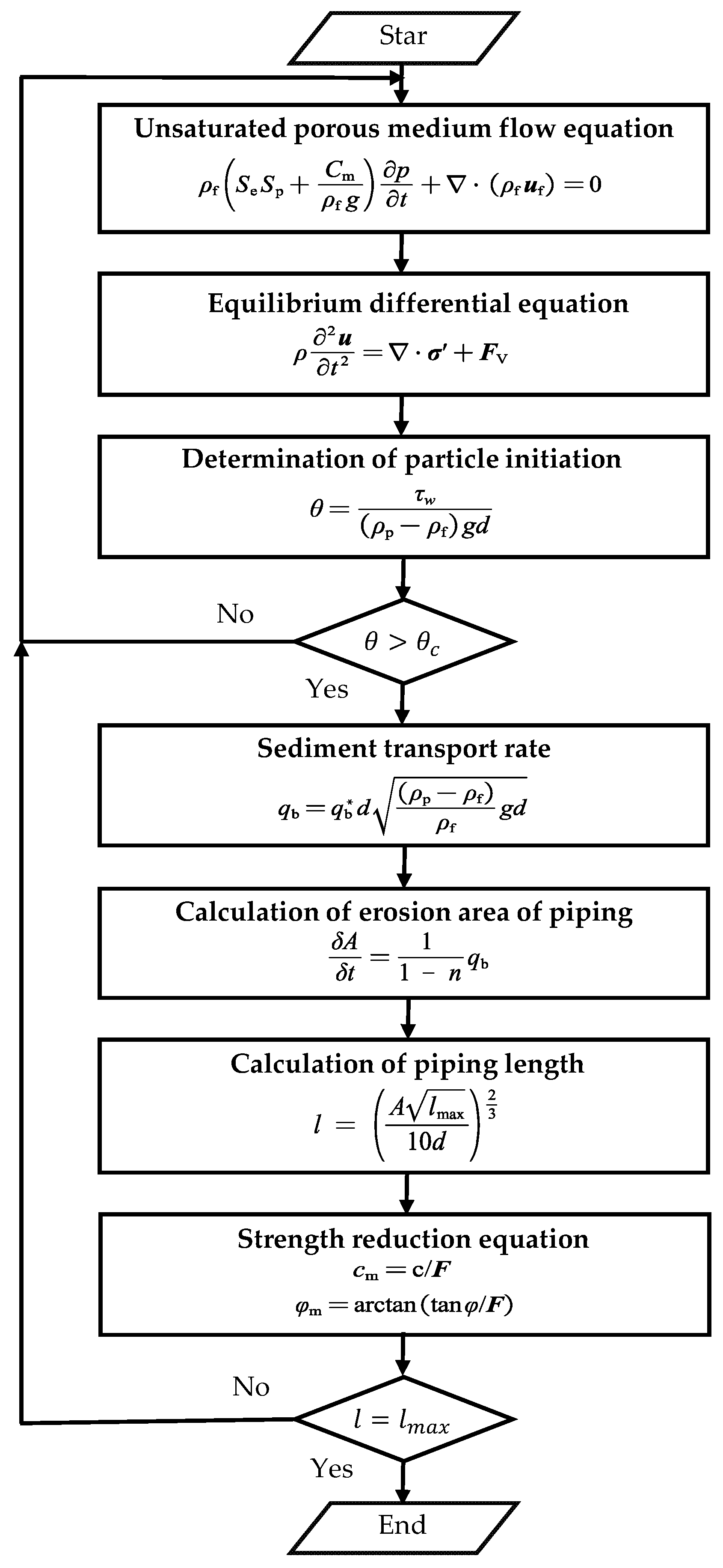
4. Numerical Computation Scheme and Validation

4.1. Numerical Simulation Approach

The numerical simulations in this study were conducted using COMSOL Multiphysics. The finite element method implemented in COMSOL Multiphysics is the Galerkin method. The Exner’s equation was calculated using the global ordinary differential equation (ODE). This time dependence was solved using an implicit backward differentiation formula (BDF). The rest of the model was solved with the direct algorithm Multifrontal Massively Parallel sparse direct Solver (MUMPS). The complete computational workflow of the numerical simulations is illustrated in Figure 1.

4.2. Validation of the Piping Model

The improved piping model was validated by comparing the simulated results with data from the IJkdijk [40] experiment. The experimental model was 25 m wide and 6.5 m high. It was composed of a sandy foundation with the height of 3 m and a dike with a width of 15 m and a height of 3.5 m. Based on experimental model data, a computational model was developed using the COMSOL 6.1 software. Figure 2 is the grid model constructed based on the IJkdijk experimental data. The region near the interface between the dike body and the dike foundation was identified as a potential location for piping, and the mesh of this area was refined accordingly. In Figure 2, the arrows indicate the upstream and downstream boundary conditions, while the blue boundaries represent impermeable conditions, i.e., no-flow boundary conditions. The upstream boundary was a gradually rising head boundary, as shown in H in Figure 3. The downstream was a boundary of fixed water level at 10 cm to ensure saturation of the dike foundation. The downstream water level was set as the reference level. The seepage on the downstream slope surface was weak; therefore, the downstream slope could be considered as a no-flow boundary. The model parameters were sourced from the IJkdijk experiment and Wewer’s paper. The dynamic viscosity was $1.236\times {10}^{-6}{ \mathrm{m}}^2/\mathrm{s}$, the particle density was $2650{ \mathrm{kg}/\mathrm{m}}^3$, the initial permeability was $1.76\times {10}^{-11}{ \mathrm{m}}^2$, the fluid density was $1000{ \mathrm{kg}/\mathrm{m}}^3$, the particle compressibility was $1\times {10}^{-8}1/P\mathrm{a}$, the fluid compressibility was 0, and the porosity was 0.37.

The piping outlet was located at the downstream toe of the dike. Figure 3 depicts the evolution of pipe length over time, with the black line representing the simulation results of this study, the red line representing the results from the IJkdijk test, and the green line representing the results from Wewer. As observed in Figure 3, the piping started to develop at 20 h and reached the upstream at 100 h in the results from Wewer. However, the piping simulated by the improved model began development at 25 h, initially progressing at a slower rate, then accelerating after 60 h, and ultimately reaching the upstream end around 80 h. Comparing the results from Wewer and the improved model with IJkdijk’s experiment, the proposed improved piping model demonstrated higher accuracy in describing the development of piping.

Figure 4 illustrates the variation in pore pressure at the monitoring point located at the center of the dike. It can be observed that after 71 h, there was a significant decrease in pore pressure. This was attributed to the development of piping reaching the monitoring point location at this time, causing the pressure head in the soil to transform into a velocity head, thereby releasing pore pressure and leading to its reduction. At 80 h, when the erosion channel was fully developed, and direct connection with the upstream was established, the pore pressure at the monitoring point tended to approach the level of the upstream water surface, resulting in an increase in pressure at the monitoring point.

From Figure 4, it can be observed that in the early stages of piping development, the numerical simulation results were consistent with the those of IJkdijk experiment. However, in the later stages of pipe development, the time at which the pore pressure at the monitoring point began to decrease in the Wewer’s result was earlier than that in the IJkdijk experiment. The result of the improved model was in closer agreement with the experiment result; however, the subsequent rise in pore pressure occurred earlier than in the experiment results. This discrepancy was attributed to the consideration of unsaturated seepage in the dike body in our model, leading to an excessively rapid erosion rate in the later stages of piping. Consequently, the erosion channel reached the upstream in a shorter time period, resulting in the earlier occurrence of pore pressure rise.

In summary, the proposed improved model demonstrated a good agreement between its simulation results and the experimental data. This confirms the reliability of the model in simulating piping.

5. Analysis of the Evolution of Piping and Its Impact on the Stability of the Dike Slope

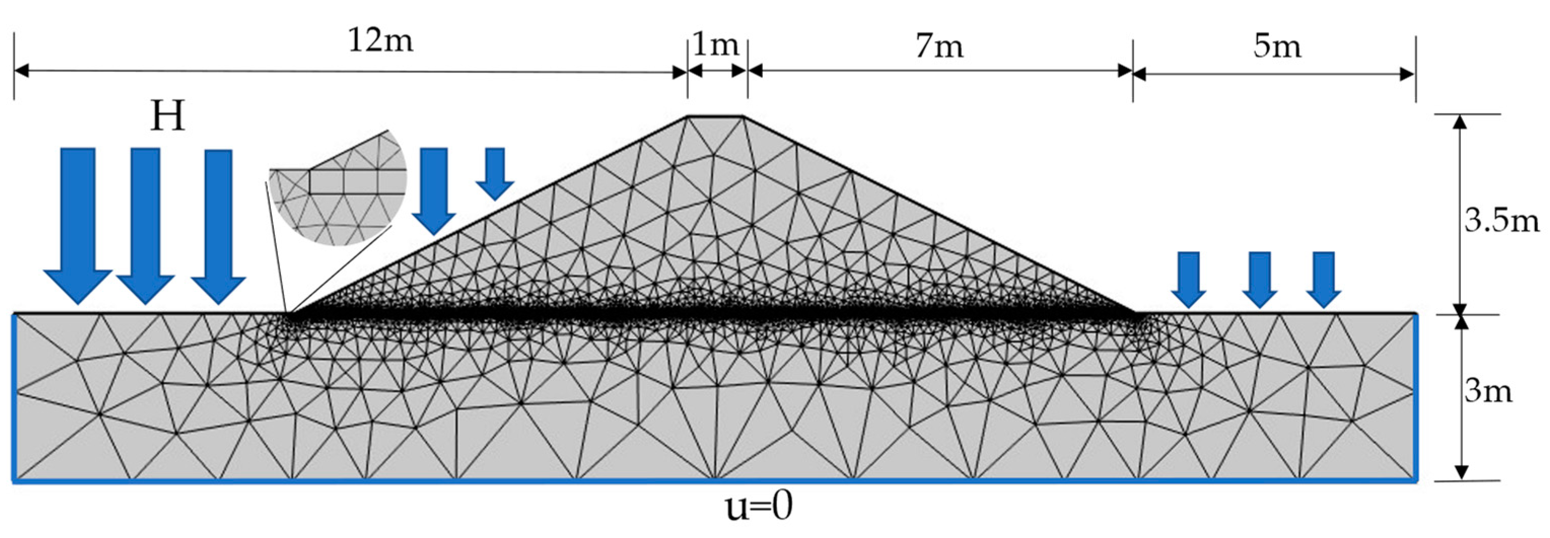
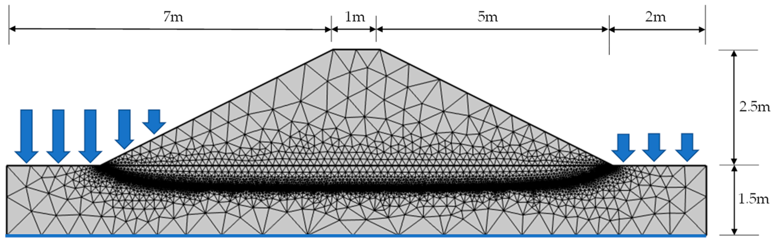
5.1. Calculation Model and Parameter Selection

A scaled-down model of the typical dike structure was constructed using COMSOL finite element software, as illustrated in Figure 5. The model was 4 m high and 15 m wide, and composed of a dike body with a height of 2.5 m and a length of 11 m, discretized into 150,000 triangular elements. The dike foundation soil consisted of clay and natural sandy soil layers, with model parameters listed as shown in

Table 1. Model parameters.

Parameter	Symbol	Value
Porosity (dike body)	$n_{\mathrm{d}}$	0.5
Porosity (clay)	$n_{\mathrm{c}}$	0.25
Porosity (soil)	$n_s$	0.37
Kinematic viscosity	$v$	$1.236 \times {{10}^{-}}^6 \left({\mathrm{m}}^2/\mathrm{s}\right)$
Particle density	${\rho }_{\mathrm{p}}$	$2650 \left({\mathrm{kg}/\mathrm{m}}^3\right)$
Fluid density	${\rho }_{\mathrm{f}}$	$1000 \left({\mathrm{kg}/\mathrm{m}}^3\right)$
Particle compressibility coefficient	${\chi }_{\mathrm{p}}$	$1 \times {{10}^{-}}^8 (1/\mathrm{Pa})$
Fluid compressibility coefficient	${\chi }_{\mathrm{f}}$	$0 (1/\mathrm{Pa})$
Cohesive strength (dike body)	$c_{\mathrm{d}}$	$2500 (\mathrm{Pa}$)
Internal friction angle (dike body)	${\phi }_{\mathrm{d}}$	24 (°)
Cohesive strength (soil)	$c_{\mathrm{s}}$	$30,000 (\mathrm{Pa}$)
Internal friction angle (soil)	${\phi }_{\mathrm{d}}$	40 (°)

.

The bottom boundary of the dike foundation was impermeable. The seepage on the downstream slope surface was weak; therefore, the downstream slope could be considered a no-flow boundary. The boundaries on both sides of the dike foundation were head boundaries, maintaining consistent heads with the groundwater level. The head at the upstream boundary was 2.2 m. The downstream was a boundary of fixed water level at 10 cm to ensure saturation of the dike foundation, with the downstream head serving as the reference plane (0 elevation).

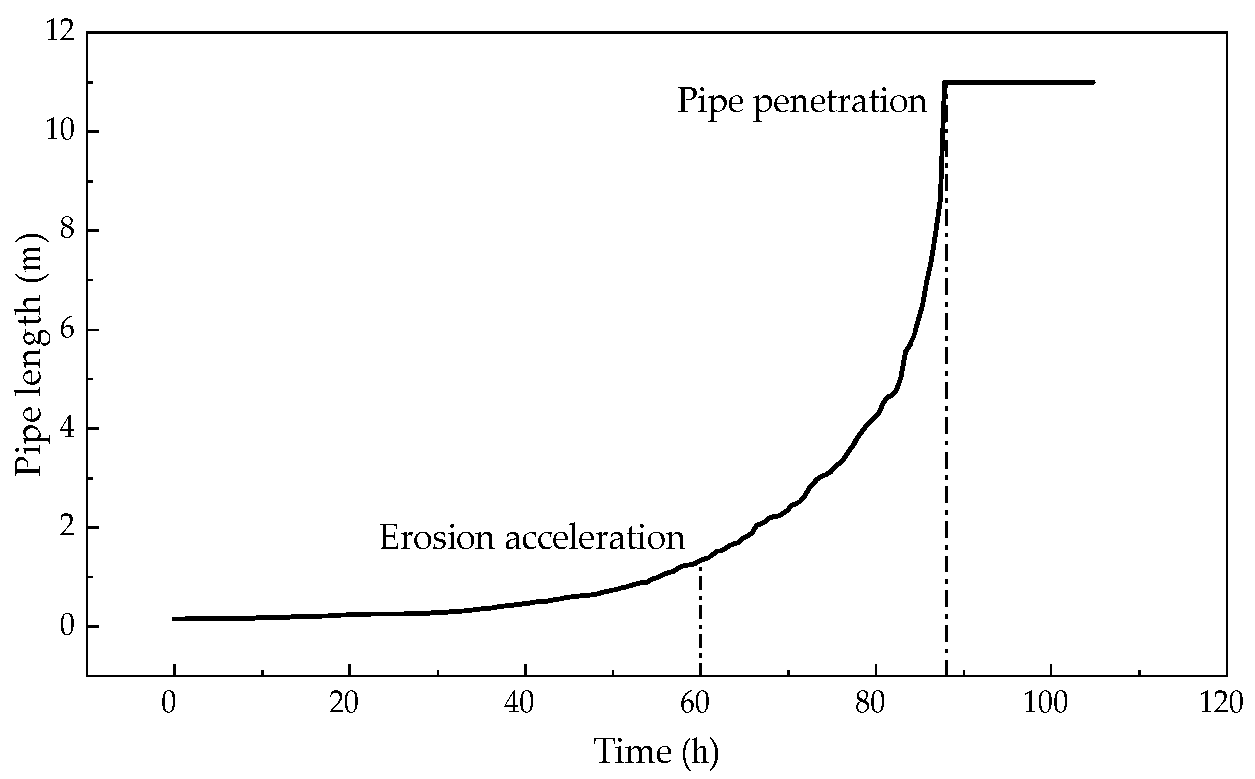
5.2. Development of Piping

Figure 6 depicts the variation in pipe length over time. As time increased, the pipe length initially showed a slowly increasing trend, followed by a significant increase in the growth rate of pipe length. In the final stage of piping, the erosion channel developed very rapidly. This phenomenon occurred due to the relatively small erosive force in the early stages of piping. However, as the erosion channel progressed upstream, the front end of the erosion channel approached the upstream boundary, resulting in larger local hydraulic gradients. These local hydraulic gradients directly influenced the erosion rate, leading to a significant increase in the rate of development of the erosion channel.

5.3. Analysis of Dike Seepage and Deformation

The formation of the erosion channel led to the emergence of easily flowing pathways in the dike base, subsequently affecting the seepage within the dike. Figure 7 illustrate the groundwater flow situation within the dike at 60 h and 82 h, respectively. It can be observed that groundwater converged at the locations where piping occurred and flowed downstream along the erosion channel. This phenomenon arose because the pressure within the erosion channel was lower than the pore pressure in the surrounding soil. As a result of this pressure difference, groundwater in the surrounding soil spontaneously flowed towards the erosion channel, creating easily flowing pathways.

The development of piping can lead to settlement at the downstream toe of the dike, causing displacement of the entire dike towards the downstream direction, as illustrated in Figure 8. This phenomenon occurs because, during the development of piping, the loss of soil particles results in the erosion of soil surrounding the erosion channel, thereby reducing the mechanical properties of the soil. Consequently, under the influence of gravity, settlement occurs in the dike. This phenomenon was particularly pronounced at the location of the piping outlet.

5.4. Analysis of dike Stability

Figure 9 shows the stability analysis results of the dike at 88 h. In this figure, (a) represents the failure slip surface of the dike slope calculated using the method of strength reduction, while (b) indicates the displacement of the dike instability failure area. It can be observed that under high-water conditions upstream, the plastic zone appeared near the downstream slope, leading to instability and failure of the downstream slope.

As shown in the Figure 10, from 87.5 h to 88 h, the erosion channel reached the upstream, and the safety factor of the dike slope dropped sharply from 1.54 to 1.488. The variation in safety factor indicates a significant change in the stability of the dike slope before and after the erosion channel penetration. As mentioned earlier, this phenomenon occurred because, after the erosion channel reached the upstream, the internal water of the pipe directly connected with the river water, causing changes in pore pressure inside the dike and consequently impacting its stability.

The above results indicate that the development of piping can cause deformation and settlement of the dike. The formation of a complete erosion channel led to a significant decrease in the stability of the slope, thereby increasing the risk of slope instability and landslides in the dike.

5.5. Analysis of Piping Development and Dike Stability under Water-Level Changes

To simulate the impact of water-level decrease after the end of the flood season on the development of piping and dike stability, modifications were made to the model boundary conditions in this section. Specifically, the upstream water head was uniformly decreased from 2.2 m to 1 m within one day, while keeping other settings unchanged. The evolution of piping in the dike foundation and the changes in the stability of dike slope during the water level decrease were computed. Figure 11 illustrates the development of the pipe length when the water level changed.

From the Figure 11, the development of piping was rapid within the first day, which was attributed to the initially high level upstream, leading to a large local hydraulic gradient within the dike. Following the decrease in water level, starting from the second day, the length of the pipe enters a phase of gradual growth, with the rate of length increase accelerating over time. The trend of erosion channel development during this phase was similar to that simulated during high water levels. By the thirteenth day, the length of piping channel reached 3.85 m and ceased to grow, indicating the cessation of piping at this point. This cessation was attributed to the reduction in hydraulic gradient caused by the low upstream water level. This led to a decrease in wall shear stress and insufficient erosive force to transport soil particles. This cessation phenomenon aligned with the piping theory proposed by Mao et al. [4], based on experimental studies. According to this theory, in certain BEPs, the erosion channel may stop developing due to the influence of hydraulic and soil conditions.

Figure 12 illustrates the displacement of dike slope instability and the distribution of plastic zones on the first day. In contrast to the high-water situation, instability and failure of the dike occurred on the water-facing side, which was attributed to the lag in the change in groundwater level within the dike. As depicted in Figure 13, the pressure head and saturation near the upstream slope were reduced due to changes in the river water level. However, the pressure head inside the dike did not decrease synchronously with the external water level. Consequently, a hydraulic gradient towards the exterior of the dike occurred due to the disparity in water levels inside and outside the dike, affecting the stress state of the dike and rendering the water-facing slope more susceptible to instability.

6. Conclusions

This paper proposes an improved model for analyzing the stability of dike slopes considering the impact of BEP. Using the improved model, the development of piping within dikes under high-water-level and water-level-drop conditions was simulated. Meanwhile, the paper also investigated the impact of BEP on pore pressure, seepage distribution, and the stability of the dike slope. The main conclusions were as follows:

(1)

After adding the seepage field of the dike body, the development trend of the piping channel became more consistent with the experimental result, proving that the seepage field of the dike body indeed affected the development of BEP. By comparing the simulation results, this study concluded that the rapid development of pipe in the final stages of BEP is related to the seepage of the dike body.

(2)

BEP will influence the seepage distribution of the dike and promote the convergence of groundwater in the piping channel. After the piping channel was penetrated, the safety factor of the dike significantly decreased, indicating that the penetration of pipe will significantly reduce the stability of the dike.

(3)

In situations where the water levels drops suddenly, BEP will stop developing due to factors such as hydraulic conditions. In this situation, due to the influence of the water level difference, the instability will occur on the upstream slope of the dike.

This study simulated the development of piping channels and the deformation of dikes, investigating the impact of BEP on the stability of the dike. In addition, we also studied the development of piping channels and the instability of the dike in conditions of water-level drop. The improved model does not consider the collapse of the soil above the pipe during BEP. Additionally, we did not comprehensively assess the impact of BEP on dike stability, ignoring changes in soil parameters such as Young’s modulus. Further research into these aspects may be conducted in future work.

References

1. Riha, J.; Petrula, L. Experimental research on backward erosion piping progression. Water 2023, 15, 2749. [Google Scholar] [CrossRef]
2. Okamura, M.; Tsuyuguchi, Y.; Izumi, N.; Maeda, K. Centrifuge modeling of scale effect on hydraulic gradient of backward erosion piping in uniform aquifer under river levees. Soils Found. 2022, 62, 101214. [Google Scholar] [CrossRef]
3. Terzaghi, K. Der Grundbruch an Stauwerken und Seine Verhutung. Wasserkraft 1922, 17, 445–449. [Google Scholar]
4. Mao, C.X.; Duan, X.B.; Cai, J.B.; Ru, J.H. Experimental study on harmless seepage piping in levee foundation. J. Hydraul. Eng. 2004, 11, 46–53+61. [Google Scholar]
5. Ojha, C.S.P.; Singh, V.P.; Adrian, D.D. Influence of Porosity on Piping Models of Levee Failure. J. Geotech. Geoenviron. Eng. 2001, 127, 1071–1074. [Google Scholar] [CrossRef]
6. Ovalle-Villamil, W.; Sasanakul, I. Centrifuge Modeling Study of Backward Erosion Piping with Variable Exit Size. J. Geotech. Geoenviron. Eng. 2021, 147, 04021114. [Google Scholar] [CrossRef]
7. Zheng, G.; Tong, J.B.; Zhang, T.; Wang, Z.W.; Li, X.; Zhang, J.Q.; Qi, C.Y.; Zhou, H.; Diao, Y. Visualizing the dynamic progression of backward erosion piping in a Hele-Shaw cell. J. Zhejiang Univ. Sci. A 2022, 23, 945–954. [Google Scholar] [CrossRef]
8. Liang, Y.; Yu, J.T.; Zhang, Q.; Xu, B.; Zhang, H.J.; Gong, S.Y. Experimental study on the effect of skeleton particle composition on piping law of cohesionless soil. J. Hohai Univ. (Nat. Sci.) 2024, 52, 63–69. [Google Scholar]
9. Ovalle-Villamil, W.; Sasanakul, I. Influence of Seepage Length on Backward Erosion Piping Behaviors in Centrifuge Model Testing. J. Geotech. Geoenviron. Eng. 2022, 148, 04022102. [Google Scholar] [CrossRef]
10. Wang, Z.; Oskay, C.; Fascetti, A. Three-dimensional numerical modeling of the temporal evolution of backward erosion piping. Comput. Geotech. 2024, 171, 106381. [Google Scholar] [CrossRef]
11. Wang, D.; Fu, X.; Jie, Y.X.; Dong, W.; Hu, D. Simulation of pipe progression in a levee foundation with coupled seepage and pipe flow domains. Soils Found. 2014, 54, 974–984. [Google Scholar] [CrossRef]
12. Rosenbrand, E.; van Beek, V.; Bezuijen, A. Numerical modelling of the resistance of the coarse sand barrier against backward erosion piping. Géotechnique 2021, 72, 522–531. [Google Scholar] [CrossRef]
13. Rotunno, A.; Callari, C.; Froiio, F. A finite element method for localized erosion in porous media with applications to backward piping in levees. Int. J. Numer. Anal. Methods Geomech. 2018, 43, 293–316. [Google Scholar] [CrossRef]
14. Froiio, F.; Callari, C.; Rotunno, A.F. A numerical experiment of backward erosion piping: Kinematics and micromechanics. Meccanica 2019, 54, 2099–2117. [Google Scholar] [CrossRef]
15. Vandenboer, K.; van Beek, V.; Bezuijen, A. 3D finite element method (FEM) simulation of groundwater flow during backward erosion piping. Front. Struct. Civ. Eng. 2014, 8, 160–166. [Google Scholar] [CrossRef]
16. Robbins, B.; Griffiths, D. A two-dimensional, adaptive finite element approach for simulation of backward erosion piping. Comput. Geotech. 2020, 129, 103820. [Google Scholar] [CrossRef]
17. Wang, Y.; Ni, X. Hydro-mechanical analysis of piping erosion based on similarity criterion at micro-level by PFC3D. Eur. J. Environ. Civ. Eng. 2013, 17, s187–s204. [Google Scholar] [CrossRef]
18. Nie, Y.P.; Sun, D.Y.; Wang, X.K. Quantitative analysis of the erosion process in horizontal cobble and gravel embankment piping via CFD-DEM coupling method. J. Braz. Soc. Mech. Sci. Eng. 2022, 44, 610. [Google Scholar] [CrossRef]
19. Lominé, F.; Scholtès, L.; Sibille, L.; Poullain, P. Modeling of fluid-solid interaction in granular media with coupled lattice Boltzmann/discrete element methods: Application to piping erosion. Int. J. Numer. Anal. Methods Geomech. 2013, 37, 577–596. [Google Scholar] [CrossRef]
20. Duc Kien, T.; Prime, N.; Froiio, F.; Callari, C.; Vincens, E. Numerical modelling of backward front propagation in piping erosion by DEM-LBM coupling. Eur. J. Environ. Civ. Eng. 2016, 21, 960–987. [Google Scholar]
21. Sibille, L.; Marot, D.; Poullain, P.; Lominé, F. Phenomenological interpretation of internal erosion in granular soils from a discrete fluid-solid numerical model. In Proceedings of the 8th International Conference on Scour and Erosion, Oxford, UK, 12–15 September 2016; CRC Press: Oxford, UK, 2016. [Google Scholar]
22. Zhang, X.; Wang, C.Y.; Wong, H.; Tong, J.; Dong, J. Modeling dam deformation in the early stage of internal seepage erosion—Application to the teton dam, Idaho, before the 1976 Incident. J. Hydrol. 2021, 605, 127378. [Google Scholar] [CrossRef]
23. Zhou, X.J.; Jie, Y.X.; Li, G.X. Numerical simulation of piping based on coupling seepage and pipe flow. Rock Soil Mech. 2009, 30, 3154–3158. [Google Scholar]
24. Zhou, X.J.; Jie, Y.X.; Li, G.X. Numerical simulation of piping in levee. J. Hydroelectr. Eng. 2011, 30, 100–106. [Google Scholar]
25. van Beek, V.; Robbins, B.; Rosenbrand, E.; Esch, J. 3D modelling of backward erosion piping experiments. Geomech. Energy Environ. 2022, 31, 100375. [Google Scholar] [CrossRef]
26. Robbins, B.; van Beek, V.; Pol, J.; Griffiths, D. Errors in finite element analysis of backward erosion piping. Geomech. Energy Environ. 2022, 31, 100331. [Google Scholar] [CrossRef]
27. van Beek, V.; Robbins, B.; Hoffmans, G.; Bezuijen, A.; Rijn, L. Use of incipient motion data for backward erosion piping models. Int. J. Sediment Res. 2019, 34, 401–408. [Google Scholar] [CrossRef]
28. Wewer, M.; Aguilar López, J.P.; Kok, M.; Bogaard, T. A transient backward erosion piping model based on laminar flow transport equations. Comput. Geotech. 2021, 132, 103992. [Google Scholar] [CrossRef]
29. Ahmed, Z.; Wang, S.; Jasim, O.H.; Xu, Y.; Wang, P. Variability effect of strength and geometric parameters on the stability factor of failure surfaces of rock slope by numerical analysis. Arab. J. Geosci. 2020, 13, 1112. [Google Scholar] [CrossRef]
30. Sarma, S.K. Stability analysis of embankments and slopes. Geotechnique 1973, 23, 423–433. [Google Scholar] [CrossRef]
31. Qi, X.; Li, D. Effect of spatial variability of shear strength parameters on critical slip surfaces of slopes. Eng. Geol. 2018, 239, 41–49. [Google Scholar] [CrossRef]
32. Clough, R.W.; Woodward, R.J. Analysis of embankment stresses and deformations. J. Soil Mech. Found. Div. 1967, 93, 529–549. [Google Scholar] [CrossRef]
33. Li, Q.D.; Xiao, T.; Cao, Z.J.; Tang, X.S.; Fang, G.G. Auxiliary slope reliability analysis using limit equilibrium method and finite element method. Chin. J. Geotech. Eng. 2016, 38, 1004–1013. [Google Scholar]
34. Ahmed, Z.; Yousuf, S.; Wang, S.; Rehman, S.U.; Gul, M.; Hanif, M.S. An Artificial Neural Network Method for Forecasting the Stability of Soil Slopes. Proc. Pak. Acad. Sci. A Phys. Comput. Sci. 2024, 61, 11–18. [Google Scholar]
35. Ke, L.; Takahashi, A. Strength reduction of cohesionless soil due to internal erosion induced by one-dimensional upward seepage flow. Soils Found. 2012, 52, 698–711. [Google Scholar] [CrossRef]
36. Liu, Q.Q.; Li, J.C. Effects of water seepage on the stability of soil-slopes. Procedia IUTAM 2015, 17, 29–39. [Google Scholar] [CrossRef]
37. Zhang, L.; Wu, F.; Zhang, H.; Zhang, L.; Zhang, J. Influences of internal erosion on infiltration and slope stability. Bull. Eng. Geol. Environ. 2019, 78, 1815–1827. [Google Scholar] [CrossRef]
38. Rahimi, M.; Shafieezadeh, A. Coupled backward erosion piping and slope instability performance model for levees. Transp. Geotech. 2020, 24, 100394. [Google Scholar] [CrossRef]
39. van Esch, J.M.; Sellmeijer, J.B.; Stolle, D. Modeling transient groundwater flow and piping under dikes and dams. In Third International Symposium on Computational Geomechanics (ComGeo III); Taylor I& Francis: Krakow, Poland, 2013. [Google Scholar]
40. Koelewijn, A.R.; Pals, N.; Sas, M.J.; Zomer, W.S. Ljkdijk Piping Experiment: Validatie van Sensor-en Meettechnologie Voor Detectie van Optreden van Piping in Waterkeringen. Stowa Rapport. 2011. Available online: https://repository.tudelft.nl/islandora/object/uuid:2d43fe32-0e1a-4543-8536-5156ab007261 (accessed on 1 June 2022.).
41. Van Genuchten, M. A closed-form equation for predicting the hydraulic conductivity of unsaturated soils. Soil Sci. Soc. Am. J. 1980, 44, 892–898. [Google Scholar] [CrossRef]
42. Yalin, M.S.; Karahan, E. Inception of Sediment Transport. J. Hydraul. Div. 1979, 105, 1433–1443. [Google Scholar] [CrossRef]
Figure 1. Methodology flow chart.
Water 16 01706 g001
Figure 2. Grid model of dike body and foundation.
Water 16 01706 g002
Figure 3. Upstream hydraulic head and comparison of pipe length development [28,40].
Water 16 01706 g003
Figure 4. Comparison of pore pressure at central detection points [28,40].
Water 16 01706 g004
Figure 5. Grid model of a typical dike.
Water 16 01706 g005
Figure 6. Pipe length development.
Water 16 01706 g006
Figure 7. The distribution of seepage inside the dike during the development of piping: (a) distribution of seepage inside the dike at 60 h and (b) distribution of seepage inside the dike at 82 h.
Water 16 01706 g007
Figure 8. Total displacement of dike during piping development (m) (amplification factor of 1500).
Water 16 01706 g008
Figure 9. The stability analysis results of dike slope at 88 h: (a) dangerous sliding surface (equivalent plastic strain) and (b) total displacement of the instability zone (m).
Water 16 01706 g009
Figure 10. Safety factor of the dike slope.
Water 16 01706 g010
Figure 11. Development of the pipe when water level drops.
Water 16 01706 g011
Figure 12. The calculation results of dike slope stability after water level drop: (a) total displacement of instability zone (m) and (b) dangerous sliding surface (equivalent plastic strain).
Water 16 01706 g012
Figure 13. The unsaturated seepage state of dike after water level drop: (a) pressure−head contour of dike (m) and (b) saturation of dike.
Water 16 01706 g013