Long-Term Stability of Low-Cost IoT System for Monitoring Water Quality in Urban Rivers

Abstract

Monitoring water quality in urban rivers is crucial for water resource management since point and non-point source pollution remain a major challenge. However, traditional water quality monitoring methods are costly and limited in frequency and spatial coverage. To optimize the monitoring, techniques such as modeling have been proposed. These methods rely on networks of low-cost multiprobes integrated with IoT networks to offer continuous real-time monitoring, with sufficient spatial coverage. But challenges persist in terms of data quality. Here, we propose a framework to verify the reliability and stability of low-cost sensors, focusing on the implementation of multiparameter probes embedding six sensors. Various tests have been developed to validate these sensors. First of all, a calibration check was carried out, indicating good accuracy. We then analyzed the influence of temperature. This revealed that for the conductivity and the oxygen sensors, a temperature compensation was required, and correction coefficients were identified. Temporal stability was verified in the laboratory and in the field (from 3 h to 3 months), which helped identify the frequency of maintenance procedures. To compensate for the sensor drift, weekly calibration and cleaning were required. This paper also explores the feasibility of LoRa technology for real-time data retrieval. However, with the LoRa gateways tested, the communication distance with the sensing device did not exceed 200 m. Based on these results, we propose a validation method to verify and to assure the performance of the low-cost sensors for water quality monitoring.

1. Introduction

Monitoring the water quality of urban rivers is one of the most important issues in water resources management [1]. However water quality degradation is still problematic, due to leaky sewers, rain runoff on contaminated surfaces, and untreated wastewater discharge in surface waters during rain events [2]. The spatial and temporal monitoring of water quality in rivers is crucial to optimize the management of freshwater resources since it provides important information to guide stakeholders [3,4,5]. However for most regulatory parameters, expensive and time-consuming field collection and laboratory analysis are necessary. For instance, for the management of bathing sites, the regulatory monitoring of the bathing waters is based on the enumeration of cultivable fecal indicator bacteria following the European Bathing directive 2006/7/EC [6,7]. Such a monitoring approach is restrictive both in terms of frequency and spatial coverage, resulting in poor comprehension of the actual water quality in a particular area at a particular time [3,8].

More effective water quality control should rely on methods that are rapid and low cost with minimum sampling required, and, ultimately, it should provide real-time results [8,9,10]. In addition, in situ sensing devices combined with machine learning could help stakeholders to detect in real time the possible contamination and to optimize the sampling effort [4,5]. Cost-effective strategies should rely on few selected parameters with available low-cost sensors that will serve as indicators of water quality. As pointed out by Zhu et al. [11], there is no consensus definition of ‘low-cost’ sensors. The cheapest sensors available on the market are usually considered “low cost”, and price ranges can depend on the parameter [11]. Several physico-chemical parameters can easily be measured in situ, with sensors. For instance, Kannel et al. [12] showed the usefulness of monitoring temperature, pH, dissolved oxygen concentrations, conductivity and turbidity to assess the spatial and temporal changes of water pollution and to classify rivers according to their water quality.

A high number of low-cost sensors could be deployed in networks at large spatial scale (Internet of Things, IoT). Each individual sensing device may present a slightly greater error margin than the precision obtained with high-cost equipment. However, the multitude of sensors should compensate by increasing the amount of information both temporally and spatially [13]. The continuous development of IoT solutions based on non-proprietary methods during the last decade allows a viable real-time measurement of the water quality for a large spectrum of applications such as monitoring drinking water resources and bathing sites [14,15,16]. Many initiatives have arisen, and the interest of the research community has tremendously increased over time [17]. Real-time water quality monitoring through IoT application is expected to help reduce costs associated with logistics and increasing the number of sites monitored. However, the energy autonomy of the monitoring devices deployed on the field needs to be considered. Usually, the sensor are powered by batteries or solar cells. Data are then transmitted either using SMS or long-range (LoRA) technology. In order to be energy-efficient, the long-range (LoRA) technology offers an interesting solution, making it suitable for devices deployed over long periods of time [17,18].

Many challenges remain and need to be covered, such as the reliability, the stability and the repeatability of the measurement, the similarity of performance between sensor units and their interoperability in order to implement in the field reliable continuous monitoring of the water quality [17]. Therefore, the general objective of this paper is to propose a framework to verify the reliability and the stability of the readings and to identify the necessary maintenance of low-cost sensors in order to optimize the quality of the acquired data to assist the stakeholders in the daily management of river water.

Indeed, few studies have focused on the long-term reliability and viability of the sensors, and were restricted to a maximum of 20–30 days despite the fact that river monitoring requires longer periods [14,17,19,20,21,22,23]. As a consequence, our first objective was to analyze the stability over a longer period of 3 months.

Moreover, previous papers highlighted the need for maintenance and cleaning routines to avoid the deposition of debris and biofouling of the sensors that would impair the measurement [24,25]. However, no best-practice guideline for the calibration and validation of low-cost sensor networks exists. As the consequence, our second objective was to propose a framework for validation of low-cost sensors.

An additional crucial issue is to consider the data loss due to the limited communication distance between the sensors and the LoRa gateway [18]. As a consequence, our third objective was to test two LoRa gateways in order to determine the maximum distance between the devices and the gateway without data loss.

In order to address these three objectives, we designed a low-cost multiparameter prototype that can monitor surface water quality using IoT technology. Several sensors such as temperature, pH, conductivity, turbidity and dissolved oxygen were embedded in this device. After the calibration of each sensor, their precision and stability were analyzed in laboratory using reference solutions. The low-cost sensing device was validated for long-term monitoring in the field by comparing it with highly accurate monitoring platforms. In order to validate the possibility of using the prototype in networks, two units were compared, and the performance of the LoRA gateways was assessed.

2. Materials and Methods

To monitor water quality, we implemented a LoRa-based wireless system network which includes a LoRa gateway and a network of low-cost sensing devices with real-time data recovery (Figure 1). Arduino technology was selected to design this multiparameter sensing device. To execute instructions, process the data, and perform data transmission, two boards can be used: the Arduino UNO R3 based on the Microchip ATmega328P, or the Arduino Mega 2560 microcontroller board based on ATmega2560. The latter was chosen for its compatibility with a high number of monitoring devices [26]. Indeed, the Arduino mega board has 8 times more memory space than the UNO R3 board [26,27].

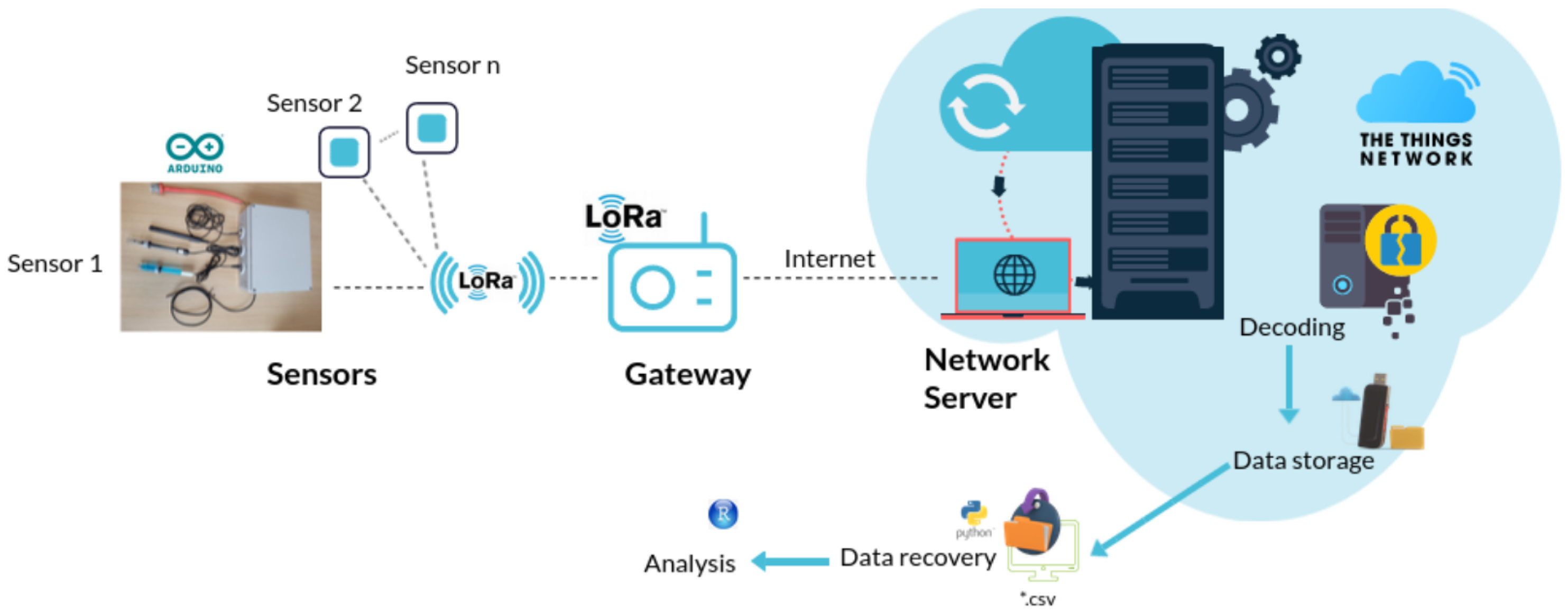
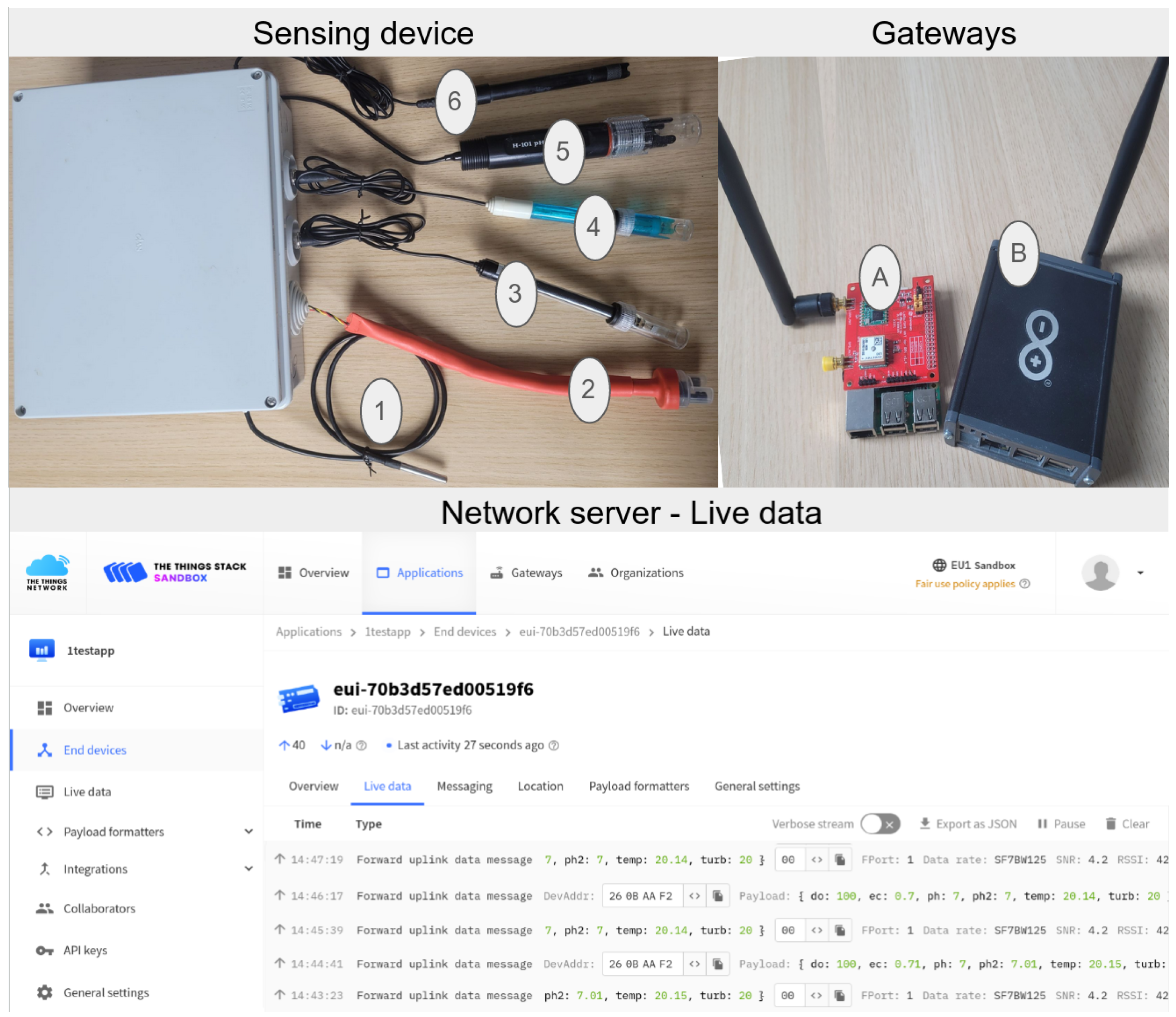
2.1. Prototype Design

Each monitoring device (called “unit”) included an external battery (20,000 mAh), 6 analog or digital sensors from DFRobot (Shanghai, China) (temperature, 2 pH, conductivity, turbidity, and dissolved oxygen), a micro SD module/card for data storage, a 16 Bit ADC module V1.0 to increase the precision of the conductivity, turbidity and dissolved oxygen sensors, and a LoRa Shield to connect to a LoRa network [28,29]. Zhu et al. [11] and Camargo et al. [17] compared a list of low-cost water quality sensors with their specifications and a summary of their performance characteristics. These studies were used to select the sensors for our device in order to have a range of reliable low-cost and medium-cost sensors [11]. No true low-cost sensors exist for monitoring nutrient concentrations, such as nitrogen and phosphorus. The cheapest from Vernier costs around EUR 300 [11]. For pH, two different types of sensors were mounted in the sensing devices in order to compare their performance, which are later named “pH-1” and “pH-2”. All parts of the system were contained in a waterproof box. Analog isolators were used to avoid any signal interference among the sensors, except for the pH sensor. The code allowing the measurement of all parameters at regular intervals was uploaded to the Arduino board and is available on GitHub (https://github.com/naloufi-manel/low_cost_sensor.git (accessed on 20 March 2024)) with the Python (version 3.8.1) and R scripts (version 4.1.1).

2.1.1. Low-Cost Sensors

The pH sensor, which measures the hydrogen ion activity in solution, comprises a pH glass electrode and a silver/silver chloride reference electrode [14]. The pH-1 sensor (SEN0161-V2, DFRobot, Shanghai, China) was cheaper than the industrial pH-2 sensor (SEN0169-V2, DFRobot, Shanghai, China).

The specific conductivity reflects the number of electrolytes dissolved in the water [30]. We selected the DFR0300 (DFRobot) sensor since it is the cheapest sensor compatible with Arduino [11]. However, its detection range may be more adapted for coastal environments than rivers (

Table 1. Characteristics and specifications of the Arduino sensors.

Parameters	Temperature [9,32] (°C)	pH-1 [33]	pH-2 [34]	Conductivity [30] (mS·cm−1)	Turbidity [35,36] (NTU)	Dissolved Oxygen [37,38] (%)
Sensor, DFRobot, Shanghai, China	DS18B20	SEN0161-V2	SEN0169-V2	DFR0300	SEN0189	SEN0237-A
Detection range	−10 to 85	0 to 14		0 to 20	0 to 1000	0 to 100
Resolution	0.010	0.010		0.001	1.000	0.050
Measurement Accuracy	±0.5	±0.5	±0.1	±1.0	±3.6	±2.0
Price (EUR)	8	39	65	70	9	148

). For the conductivity measurements, Equation (1) is commonly used to correct the measurements by comparing with a reference measurement at 25 °C:

$${\mathrm{EC}}_{25}={\displaystyle \frac{E{C}_T}{1+a(T-25)}}$$

(1)

where $E{C}_T$ is the conductivity at temperature T (°C), ${\mathrm{EC}}_{25}$ is the conductivity at 25 °C, and (°C⁻¹) is a temperature compensation factor corresponding to the percentage increase per degree [31].

For turbidity measurement, the selected sensor (SEN0189, DFRobot, Shanghai, China) measures the light transmittance and scattering rate which changes with the amount of total suspended solids [36]. The sensor uses an infrared LED as a light source and an infrared phototransistor to detect the amount of light not blocked by the water. A change in voltage is obtained and converted into unit measuring turbidity NTU (Nephelometric Turbidity unit) using Equation (2) in a range from 1 to 1000 NTU [35,36]. The upper part of the sensor is covered with a heat-shrink sheath to make it waterproof, and the sensor is shielded from external light using an opaque plastic cover [39]:

$$\mathrm{Turbidity}={\displaystyle \frac{3.9994-voltage}{0.0008}}$$

(2)

For measuring dissolved oxygen (SEN0237-A, DFRobot), we select a galvanic sensor with a filling solution and a membrane cap. Its response time stands within a few seconds. Since dissolved oxygen concentration is directly influenced by temperature, we include a temperature compensation in our code [37,38]. Equation (3) is usually used to take into account the temperature effect [37]:

$$\mathrm{DO}={\displaystyle \frac{volt+b\ast T-b\ast T_{cal}}{vol{t}_s+b\ast T-b\ast T_{cal}}}\ast 100$$

(3)

where DO is the dissolved oxygen (in saturation (%)), volt is the voltage measured at a temperature T, $vol{t}_s$ is the voltage corresponding to the saturated dissolved oxygen measured at a temperature $T_{cal}$, and b (°C⁻¹) is a temperature compensation factor [37].

2.1.2. Reference Sensors

To validate the low-cost sensors (noted Arduino sensor), we compared their readings with 2 high-end HYDROLAB Series 5 multiparameters (OTT, Aix-En-Provence, France), which embedded 4 sensors (noted OTT). For dissolved oxygen, we also compared the low-cost sensor with a MINIDOT LOGGER sensor (PME, Vista, CA, USA), which recorded data on an internal SD card [40]. The PME sensor measures dissolved oxygen concentration in water using a fluorescence method [40].

2.2. Specifications and Price

Table 1 and

Table 2. Characteristics and specifications of the Hydrolab multiprobes (OTT) [41].

Parameters	Temperature (°C)	pH	Conductivity (mS·cm−1)	Turbidity (NTU)
Detection range	−5 to 50	0 to 14	0 to 100	0 to 3000
Resolution	0.01	0.01	0.0001	0.10
Measurement Accuracy	±0.100	±0.200	±0.001	±1.000
Price (EUR)		480	380	1540

show the specifications, operating range, accuracy, and the price of each sensor. The price of the monitoring devices includes the 6 sensors prices added to EUR 159 for the total price of the other components (battery, microSD card and reader, ADC module, box, Arduino card, and isolators) and EUR 93 for the LoRa connection. The total price of each monitoring device was between EUR 285 and EUR 400. For the Hydrolab multiprobes from OTT, the price reached EUR 3050 and the PME sensor cost EUR 1775.

2.3. Cleaning and Calibration

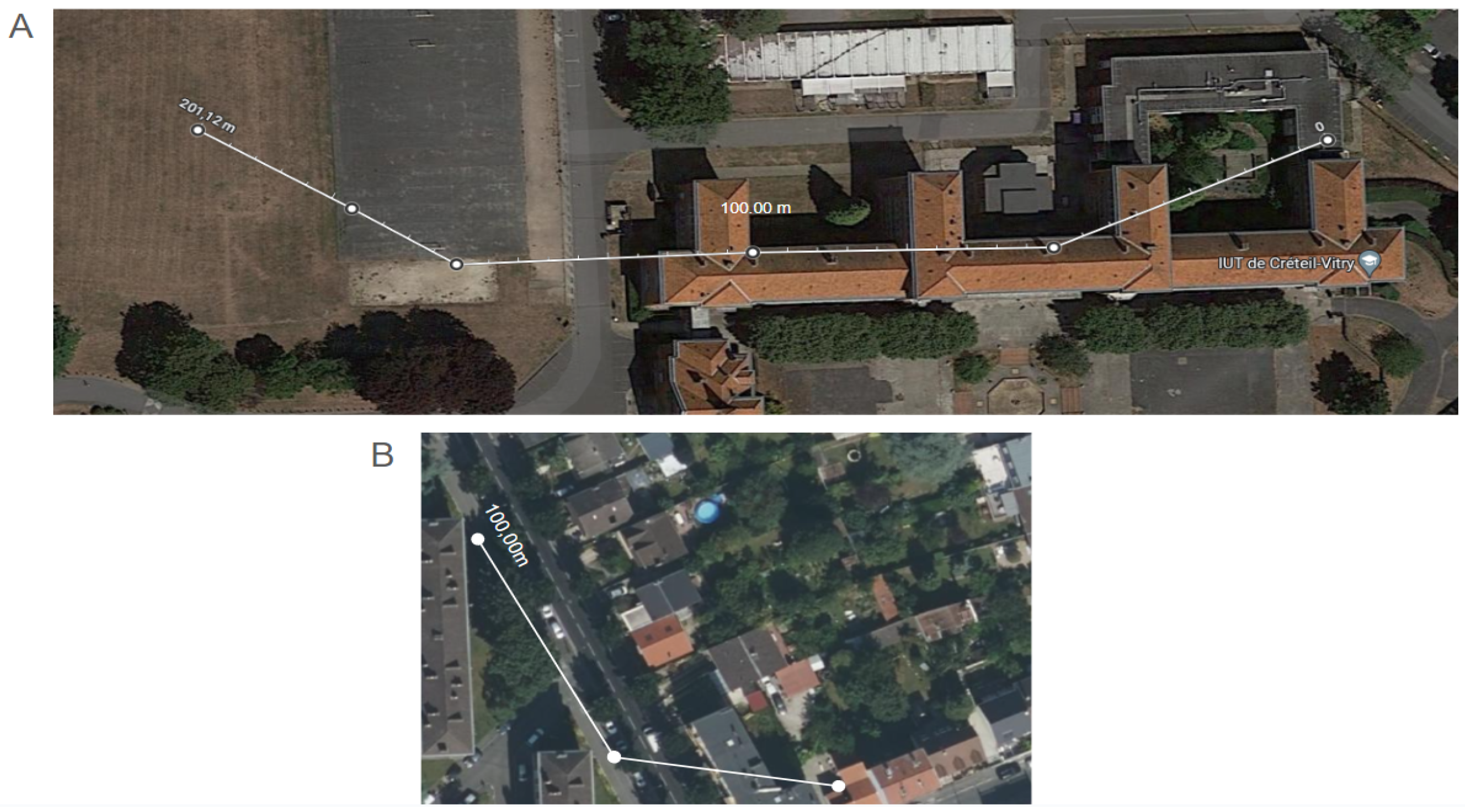
Standard solutions at different concentrations were used to calibrate each sensor except for the temperature sensor. The standard solutions were checked using an Eutech multiparameter probe for pH and conductivity, the CellOx^® 325 sensor for the dissolved oxygen and the 2100P turbidimeter (HACH) for turbidity. For the pH, we used standard buffer solutions (pH 4, 7 and 10) from VWR. To remove contamination, which leads to a reduction in slope and unstable readings, every month, the pH sensor must be immersed in 0.1 $\mathrm{mol}·{\mathrm{L}}^{-1}$ of HCL solution for a few hours then rinsed with deionized water. For conductivity, the standard solutions were prepared from a 1 M stock solution of potassium chloride. Standard solutions were diluted in deionized water to reach 0.36 $\mathrm{mS}·{\mathrm{cm}}^{-1}$, 0.72 $\mathrm{mS}·{\mathrm{cm}}^{-1}$ and 1.41 $\mathrm{mS}·{\mathrm{cm}}^{-1}$. For the turbidity sensor, we used a Formazin stock solution at 4000 NTU (prepared from dissolved hydrazine sulfate and dissolved hexamethylenetetramine). The stock solution was diluted to 0, 20 and 200 NTU in deionized water. Finally, for the dissolved oxygen sensor, a sodium sulfite solution was used for the zero point (VWR), and tapwater maintained at saturation with a bubbler served as a 100% standard solution. The oxygen sensor needed to be prepared before use by adding a filling solution into the membrane cap, which consisted of a 0.5 $\mathrm{mol}·{\mathrm{L}}^{-1}$ NaOH solution. The filling solution needed to be changed every month. Then, the sensor was calibrated at a fixed temperature (between 20 and 25 °C) in the 100% saturated water.

Each sensor was carefully washed with deionized water and wiped before calibration. The calibration took place at a fixed temperature and under agitation at 700 rpm using a magnetic stirrer. The sensor was kept in the standard solution for a few minutes to stabilize, after which the calibration point could be set. Each calibration point was measured 10 times, and the fitting regression curve (y = cx + d) was determined. For each parameter, the coefficients (c and d) were used to correct the measured values after data recovery. Calibration needed to be performed once a week.

2.4. LoRa Gateway

The LoRa Shield v1.4 from Dragino with SX1276 LoRa Chip fully compatible with Arduino models was associated with the Arduino Mega 2560, which operates at a frequency of 868 MHz (European Union) and contains an external antenna [42]. The LoRa modules were configured at a bandwidth of 125 kHz, transmit power of 14 dBm, and spread factor of 12. We tested 2 different models of the LoRa Gateway to compare their performance in terms of range coverage. The first gateway is a Raspberry gateway made of LoRa hat for RPi (Raspberry Pi) with a SX1276 LoRa Chip associated to a RPi 3 and implemented with a single-channel gateway program [43]. The second gateway is the Arduino pro Gateway LoRa connectivity. It allows up to 8 LoRa Channels in the 868 Mhz frequency (Semtech solution) and includes a microchip SX1301 with two SX1257 and an on-board UFL antenna. According to the manufacturer, LoRa gateways allow connecting devices within several kilometers [44]. For the two gateways, we estimated the spatial coverage of the gateways by measuring the distance between the end node and the gateways using a signal levels analysis. The transmission distance was tested regarding the quality of the signal by analyzing the Received Signal Strength Indicator (RSSI), the Signal-to-Noise Ratio (SNR) measured by the gateway and the time interval between the reception of 2 successive data. RSSI measures the distance between a transmitter and a receiver and SNR quantifies the strength of the signal regarding the amplitude of the ambient noise [45,46]. These indicators are commonly used for the estimation of the maximum distance [47]. The tests were performed in dense and residential urban zones (Greater Paris area), with the gateway placed at a fixed position and the end device at different positions (Figure A9).

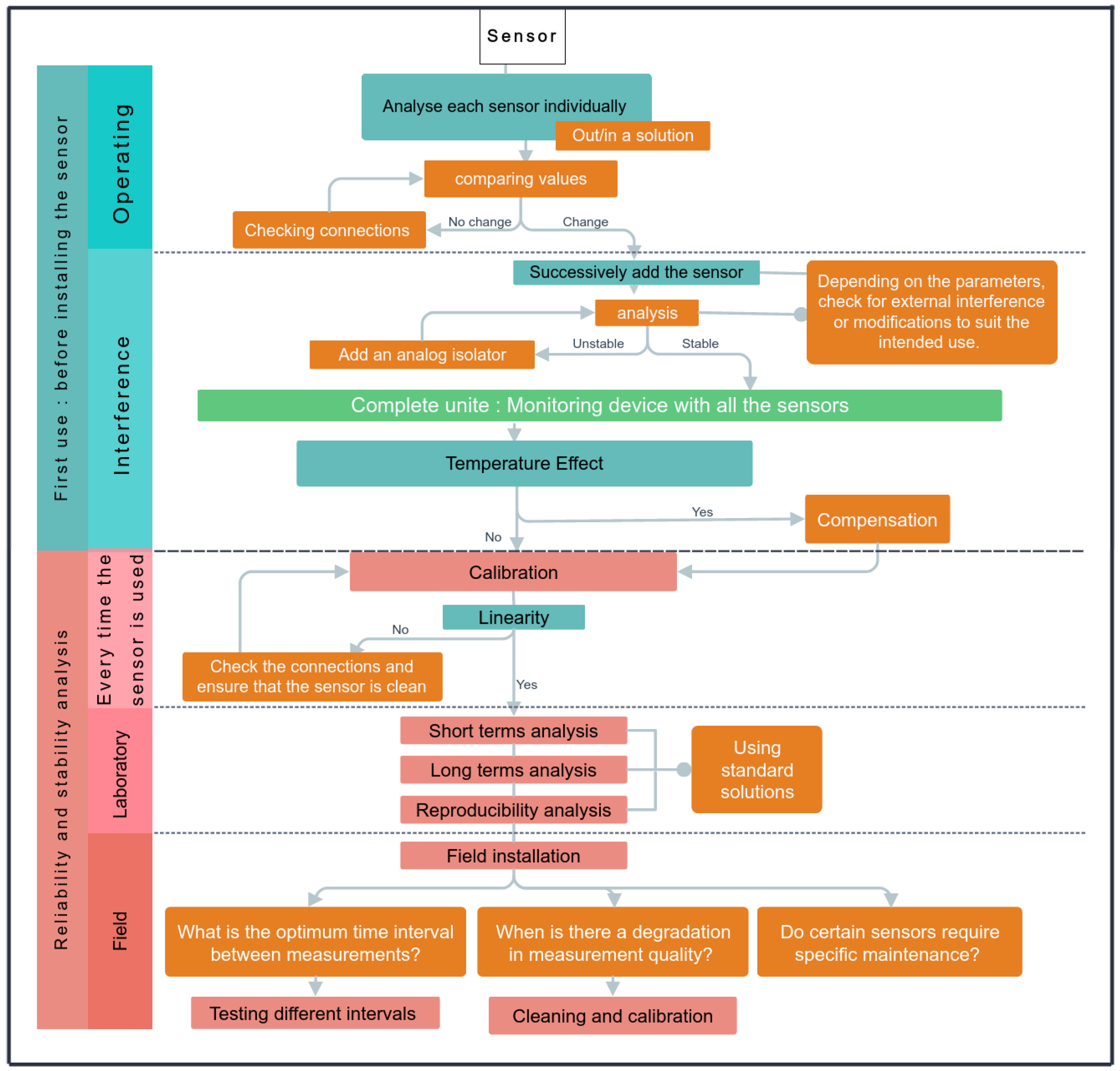
2.5. Sensor Validation

The reliability and the long-term stability of the tested low-cost sensors were checked in laboratory and in the field. The field tests were conducted in Bassin de La Villette (Paris, France), where OTT sensors were already deployed [48].

2.5.1. Accuracy

The accuracy of each sensor after a calibration was tested for 2 sensing device units in order to evaluate the linearity and the repeatability of each sensor (norm ISO 21748: 2017 and NF EN 17075 2018) [49]. The tests were performed in the laboratory at ambient temperature (20.97 ± 0.12 °C) under agitation at 700 rpm. To validate the temperature sensor, the reading was performed in a water bath with a range of temperature from 5 °C to 30 °C, incremented by 5 °C every 8 min, followed by stabilization for 15 min at the same temperature. For the other sensors, between 2 and 7 standard solutions at varying concentrations were used. For each sensors, readings were repeated 10 times for each standard solution (

Table 3. Descriptive analysis of sensors calibration for 2 units.

Parameters	Temperature (°C)	pH-1	pH-2	Conductivity (mS · cm−1)	Turbidity (NTU)	Dissolved Oxygen (%)
Number of measures (n)	368	30	30	44	77	20
Standard solutions	Temperature from 5 to 30	4, 7 and 10		4 standards from 0.22 to 1.42	7 standards from 0 to 800	0 and 100
Linearity (units 1–2)	0.999	0.999	0.999	0.998–0.993	0.998	0.999
Slope of the curve
Unit 1	0.999	0.938	0.959	1.060	0.947	1.038
Unit 2	0.999	0.950	0.984	1.083	0.916
Repeatability
Unit 1	0.01	0.02	0.01	0.02	3.66	1.74
Unit 2	0.01	0.02	0.01	0.02	3.69
Reproducibility	0.03	0.02	0.01	0.02	3.54

). Repeatability was estimated by calculating the standard deviation of the sensor’s measurements during the repeated trials. Trueness and linearity were evaluated by comparing the readings with the value of the standard solutions (true value). A linear regression was generated by plotting the low-cost sensor measurements against the known concentration of the standard solutions. Reproducibility of the sensing devices was evaluated by inter-comparison of the performance of two sensing devices. For each sensor, 2 units were tested in parallel for a week with the same standard solutions. Each parameter except for oxygen (due to high-cost of the sensor) was measured every 15 min. The temperature was maintained at around 20 °C, the pH sensors were placed in a pH 4.22 solution, the conductivity sensors were placed in a 1.42 $\mathrm{mS}·{\mathrm{cm}}^{-1}$ solution and finally, the turbidity sensors were placed in a 10 NTU solution. Reproducibility was estimated by calculating the standard deviation between 2 units.

2.5.2. Temperature Effect

In order to analyze the effect of temperature on the measurement by all the sensors and to identify the correct parameters for compensation, each sensor measured every 15 min under agitation at 700 rpm a standard solution previously cooled at 10 °C, allowing the solutions to reach an ambient temperature for 3 h (from 10 to 19 °C). The standard solutions were the following: pH 10.2; conductivity 0.72 $\mathrm{mS}·{\mathrm{cm}}^{-1}$; turbidity 20 NTU; and dissolved oxygen 100% ${\mathrm{O}}_2$ saturated water via a bubbler. For dissolved oxygen, the age of the membrane cap was also taken in consideration by using a 6-month-old membrane and a new membrane. For the new membrane, the temperature variation analyzed was between 14 and 25 °C. In order to distinguish variations due to temperature fluctuations from sensor errors, the results were compared to readings of the same standard solutions at a fixed temperature of 20.97 ± 0.12 °C for 3 h.

2.5.3. Temporal Stability in the Laboratory

Testing a probe’s stability in the laboratory, where environmental conditions are tightly regulated, provides reliable test conditions [17]. The controlled conditions of the laboratory enable the probe’s readings to be compared with known standards to verify that the measurements are accurate and consistent. The short-term and long-term stability of the sensors was tested in the laboratory at a steady ambient temperature of 19 ± 2 °C. To evaluate the short-term stability, we collected 3 replicates of 1 L water samples from Créteil Lake and from the lower Marne River (Paris area, France) in April 2022. The samples were placed under agitation, and measurements were taken continuously with the sensors every 10 s for 3 to 6 h. This short-term analysis was carried out under continuous supervision in order to immediately detect any problem or rapid variations. The pH-2 was not tested, as it was bought later.

The long-term stability was analyzed by placing each sensor in a standard solution (pH: 7; conductivity: 0.72 $\mathrm{mS}·{\mathrm{cm}}^{-1}$; turbidity: 20 NTU; and dissolved oxygen: 100% ${\mathrm{O}}_2$ saturated water via a bubbler). Measurements were taken every 3 to 5 min for approximately 3 months. For dissolved oxygen, the PME sensor was used as a reference.

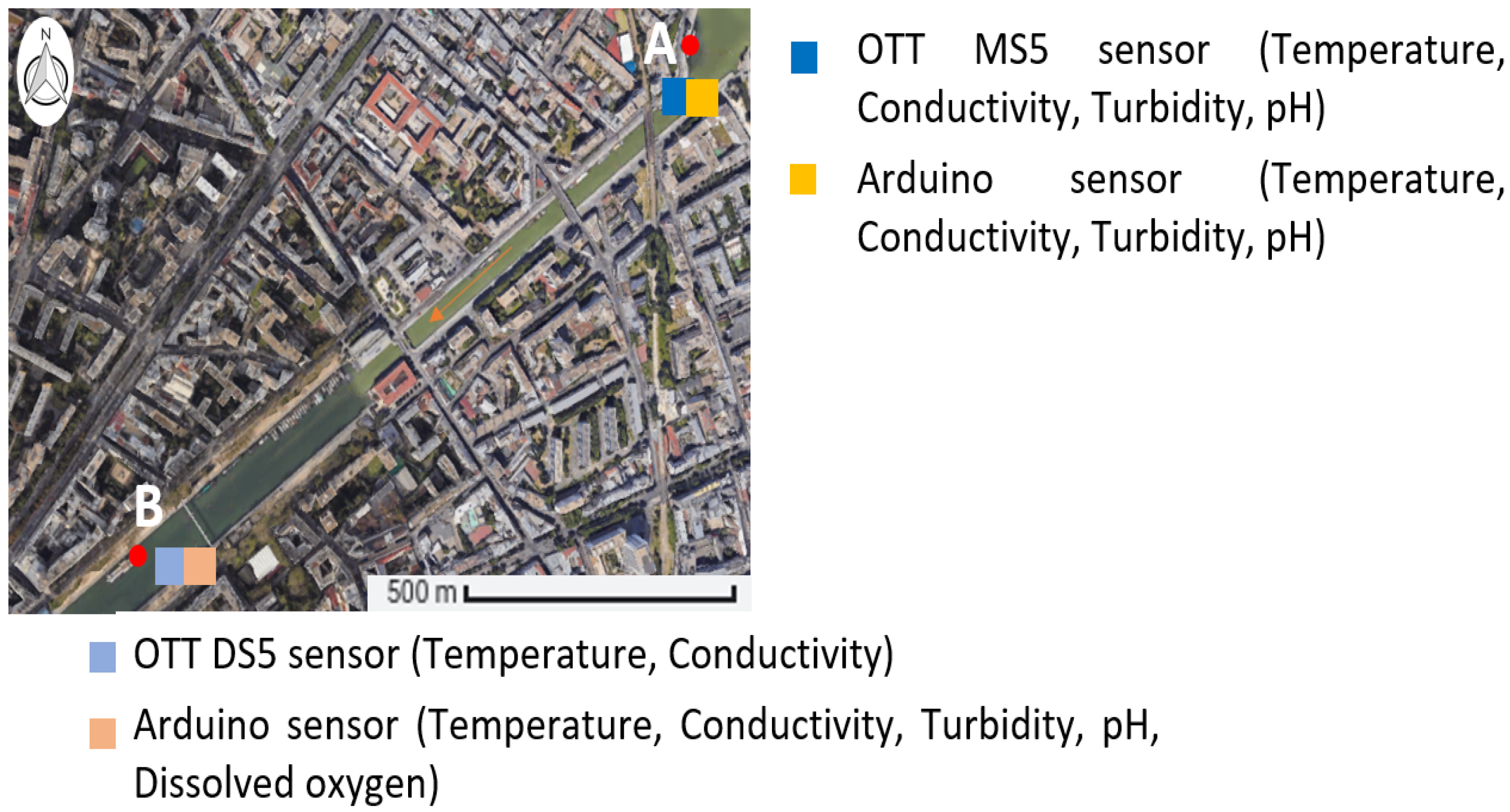
2.5.4. Temporal Stability in the Field

To test the long-term stability of the sensors in the field, we installed the low-cost monitoring devices at two sites 1 km apart from each other (A and B) at Bassin de la Villette (Paris area, France), as shown in Figure 2. Site B is in front of the bathing site of Paris Plage, and site A is upstream of site B, enabling contamination to be anticipated at the bathing site. Every year, analyses are regularly carried out by the City of Paris during the summer period (June to September) to monitor the microbiological quality in the proximity of site B. In 2022, the results indicated a good microbiological quality, with an average concentration of Escherichia coli and intestinal enterococci of 101 ± 78 MPN/100 mL and 44 ± 50 MPN/100 mL, respectively. As for the physico-chemical parameters measured, the temperature was 21.27 ± 2.83 °C, the conductivity was 0.65 ± 0.03 $\mathrm{mS}·{\mathrm{cm}}^{-1}$, and the turbidity was 7.32 ± 2.61 NTU. These 2 selected sites are part of a research project where high-precision OTT multiparameter probes have been deployed continuously since 2020. This long deployment was regularly verified and maintained in order to provide reliable data. OTT multiparameters were used as a reference. Measurements were performed in situ at site A from early September 2022 to early January 2023 and then from May 2023 to June 2023, and at site B from early September 2022 to the end of November 2022. For site B, the OTT probe only measures temperature and conductivity. Occasional loss of data occurred due to unit malfunction or installation problems on site. The installed low-cost devices were changed every week in order to clean the sensors and to check their calibration. In the beginning, cleaning and calibration were carried out directly in the field on the same unit. However, because of the length and complexity of the process starting from “15 October 2022”, the method was modified by alternating between two units each week. The sensors of device N°2 were cleaned, calibrated and stabilized for a few hours in the laboratory before replacing the device N°1 in the field, and vice versa. The measurement interval was also optimized during these stability tests.

3. Results and Discussion

Figure 3 shows a low-cost sensing device once it is completely assembled.

3.1. Accuracy of the Sensors

After calibration, the accuracy of each sensor was evaluated with the linearity and repeatability (Table 3). Correlation between measured values and the expected values of the standard solutions showed good linearity with a significant rh > 0.99 (p < 0.01) for all sensors (Figure A1). The slopes were between 0.92 and 1.08, which showed a good precision of the measure compared to the true value (Table 3). Each sensor from both devices showed high repeatability with low standard deviation values between the repeated measures, with values ranging from 0.01 to 0.02 for temperature, pH and conductivity sensors (Table 3). Turbidity and dissolved oxygen sensors showed less accuracy with higher standard deviation between repeated measures. The reproducibility between units was satisfactory for all sensors except the turbidity since measurements of the 2 sensing devices were in good agreement as demonstrated by the low standard deviation values. A recent review of Zhu et al. [11] compiled performance indicators of several low-cost sensors, including the SEN0169, DFR0300, and SEN0189 sensors selected in our study [35,39,50,51,52]. Zhu et al. [11] noticed that the information was heterogeneous and somewhat difficult to compare for trueness and linearity, and most of the time repeatability and reproducibility were not estimated.

3.2. Reproducibility of the Sensors

In order to verify if there is a difference in the accuracy of different units of the same type of sensor, a one-week experiment was carried out with two units of each sensor placed in the same standard solutions (Figure 4 and Figure A5). The temperature measurements of the two units matched almost perfectly. The average difference between the 2 units was only 0.07 °C, with a significant correlation of Spearman (Figure 4A, r = 0.98, p < 0.01, n = 434). There was fairly good reproducibility between the 2 conductivity sensors, with a mean deviation of 0.04 $\mathrm{mS}·{\mathrm{cm}}^{-1}$, a low coefficient of variation of 2.83% for unit 1 and 2.14% for unit 2 and a low but significant correlation (Figure 4B, r = 0.30, p < 0.01, n = 434).

The pH-1 sensor needed a few hours to stabilize its reading and the pH-2 meter took one day (Figure A5A,B). After stabilization, the mean deviation between the 2 units was low for both sensors (pH-1: 0.09 and pH-2: 0.02), with a low coefficient of variation for pH-1 of 0.47% for units 1 and 1.71% for unit 2 and for pH-2 0.23% for unit 1 and 0.47% for unit 2.

For the turbidity sensor, the two units differed by an average of 3.91 NTU (monitoring of a 10 NTU solution, Figure 4B). The correlation was significant but weak (r = 0.32, p < 0.01, n = 434). Figure 4B shows that the 2 units displayed the same trend over time but with a greater dispersion for the 2nd unit (coefficient of variation 29.81% for units 1 and 38.06% for units 2). The reproducibility appears rather poor for the sensor. This may be due to the difference in performance of the infrared LED and phototransistor inside the sensors [11].

3.3. Sensitivity to the Environment

Low-cost sensors are usually sensitive to the environmental conditions and need retrofit actions such as compensation equations, waterproof enclosure, or coating [11]. For instance, water temperature is known to influence the measure of some parameters and the sensitivity to sensor current [53,54]. We analyzed the effect of temperature by comparing between 3 h series of measurements under increasing temperature conditions with measurement at fixed ambient temperature. Under fixed conditions of temperature, for all of the sensors, the fluctuation over time of the measurement was low, showing a good stability of the measure. Compensation for the temperature effect was not necessary for the 2 pH meters and the turbidity sensor. The coefficients of variation of the stable temperature series for pH-1 and pH-2 meters were 0.45%, 0.22% (respectively), and 12.76% for the turbidity sensor. Under fluctuating temperature condition, the coefficients of variation were higher (0.52% and 0.47% for pH meters and 14.38% for the turbidity sensor). This slight variation as confirmed by Figure A2A,B and Figure 5A,B was rather due to random variations observed over time.

In the case of conductivity and dissolved oxygen sensors, there was a noticeable deviation in the measurement under varying temperature (3.09% and 5.88%) compared with the fixed-temperature measurements (1.60% and 0.63%) (Figure A2C,D and Figure 5C,D). This indicates that a compensation for temperature effect was required. Compensation coefficients were determined by fitting a model linear curve to the data. Several values of the ‘a’ coefficient (Equation (1)) are commonly cited in the literature. For example, Hayashi [53] reported an average a value of 0.0187 °C⁻¹ (minimum–maximum: 0.0175–0.0198 °C⁻¹), which is in accordance with the 0.019 °C⁻¹ value recommended by Clesceri and Lenore [55]. Based on the EC-temperature relation, we identified a compensation factor of 0.0265 °C⁻¹, which is comparable to the 0.025 °C⁻¹ value reported by Keller et al. [56]. After compensation of the measured values using the coefficient 0.0265 °C⁻¹, the coefficient of variation displayed a lower value (1.19%), close to the coefficient of variation obtained at a fixed temperature. The 0.0265 coefficient provided a better fit (Figure A2D) compared to the 0.0185 factor recommended by the manufacturer [30].

For the dissolved oxygen sensor, there was an effect of temperature on the readings (Figure 5C,D). This result is not surprising since the saturation of oxygen in water is dependent on the temperature and due to the change in permeability of the sensor membrane [38,57]. By fitting Equation (3) to the increasing temperature series, a factor ‘b’ of 14.48 °C⁻¹ was determined and used for the temperature compensation of the sensor signal. After compensation, the coefficient of variation decreased from 5.88% to 1.78%, which is closer to the coefficient of variation of 0.63% obtained for the reference analysis at a fixed temperature (Figure 5D). Moreover, the cap membrane should be replaced at least every 6 months since the coefficient of variation with a new membrane was 1.78%, whereas it was 7% with a membrane used for 6 months (Figure A4).

Other external factors may affect the sensing device, causing irreversible damage and reducing its lifespan. We tested if the battery was overheating the sensors housing and whether this might affect vulnerable components on the Arduino board. The manufacturer specify that Arduino boards should be operated between −25 °C and +70 °C [58]. During 3 months of monitoring temperature in the laboratory, the temperature in the box (19.97 ± 1.77 °C) and the water temperature (19.15 ± 1.91 °C) remained steady. This indicates that at ambient temperature, the battery did not overheat the waterproof box.

3.4. Temporal Stability in the Laboratory

Following calibration, a short- and long-term stability analysis was carried out with all sensors. This checking was rarely performed for the low-cost water quality sensors [11].

3.4.1. Short-Term Stability

Different surface water samples were monitored for 3 to 6 h at room temperature. The readings showed a relatively satisfactory temporal stability with average standard deviation values not significantly different from those obtained during the calibration, except for temperature (t test, n = 3, p > 0.05) (

Table 4. Short-term analysis of sensors (repeatability).

Parameters	Temperature	pH-1	pH-2	Conductivity	Turbidity	Dissolved Oxygen (%)
	(°C)			($\mathrm{mS}·{\mathrm{cm}}^{-\mathbf{1}}$)	(NTU)	Arduino Sensor	PME Sensor
Average	0.78	0.04	0.03	0.04	4.68	2.33	0.31
Min–Max	0.38–1.01	0.02–0.08	0.02–0.06	0.02–0.08	3.89–5.46	1.55–3.71	0.16–0.59

). Different studies checked the stability of DFRobot sensors using standard solutions but only for a few minutes to several hours [24,51,59,60] (and Atlas Scientific [61]). Generally speaking, in situ water measurement with low-cost sensors appears promising, with relatively satisfactory temporal stability for all parameters (temperature [59,60,61], pH [60,61], turbidity [39,59], conductivity [51,59,60,61], and dissolved oxygen [61]).

3.4.2. Detection and Removal of Outlier for Long-Term Series

The long-term stability was checked by placing each sensor in a standard solution for 3 months. The turbidity sensor showed a wide dispersion, which required rectification (Figure 6A). Indeed,the measurement of the 20 NTU standard solution gave values ranging from 0 to 1000 NTU. Filtering noise is a common pre-processing step of real-time datasets, and numerous noise-reduction methods have been used to detect and remove outliers [62,63]. A set of filtering methods was tested to identify the most optimal one: interquartile range, density-based methods K-means, DBSCAN (Density-Based Spatial Clustering of Applications with Noise) clustering, combining DBSCAN with Local Outlier Factor, Mean-shift and the ARIMA (Autoregressive Integrated Moving Average) model with the median filter approach [62,64,65,66,67].

The first five methods removed mainly extreme outliers, corresponding to 2.69% to 9.84% of the data. The ARIMA model, which can be used for data cleaning of non-stationary time series [64,67], seemed the best for cleansing this turbidity dataset (Figure 6B). With a moving window of 3, 5 and 8 points, 18.84%, 26.77% and 37.12% of the data were identified as outliers, respectively. Considering the data density and trend, the optimal window seemed to be 5, but this parameter is data-dependent [63]. The conductivity and the dissolved oxygen datasets did not require extensive cleaning since less than 0.01% and 0.001% (respectively) of the data were removed using the ARIMA approach. Time series methods are robust, and efficient data cleaning tools can process a dynamic dataset within a solid theoretical framework and detect outliers with different properties [62,68]. Since the cleaning process should be based on a minimum modification of the original data [68], for each dataset of the different sensors, different parameters were tested and retained.

3.4.3. Long-Term Stability

After cleaning of the datasets, the long-term stability was estimated using the standard deviation. Given the manufacturer’s precision values for each sensor, the calculated standard deviation values could be considered reasonable (Table 1 and

Table 5. Stability analysis of sensors: standard deviation (* without missing values during the sensor regeneration, ** values cleaned with an ARIMA method using a median filter).

Parameters	Temperature	pH-1 *	pH-2	Conductivity	Turbidity	Turbidity **	Dissolved Oxygen (%)
	(°C)			($\mathrm{mS}·{\mathrm{cm}}^{-\mathbf{1}}$)	(NTU)	(NTU)	Arduino Sensor	PME Sensor
Standard deviation	1.91	0.04	0.04	0.03	64.85	13.23	12.42	0.73

). Long-term measurements remained quite stable for most of the sensors, with the exception of turbidity and dissolved oxygen, which showed greater variability (Figure 6B and Figure 7). It could be noted that the temperature sensor correctly measured two air-conditioning incidents in the laboratory in early November and early December (Figure 7A).

Figure 7B shows that both pH meters were fairly stable (standard deviations of 0.04). However, after 3 months, the pH-1 meter drifted by 1.0 pH unit (Figure 7B). This was due to the fouling of the electrode which was removed by soaking the sensor in a 0.1 M solution of HCl for at least 8 h to a maximum of 24 h [33]. After regeneration at the end of December, the pH-1 meter was back to a stable reading (Figure 7B). The pH-2 meter is more suitable for long-term online detection due to its ring PTFE membrane that confers resistance to clogging [34].

For the conductivity sensor, only minor variations could be observed (Figure 7C). A sharp decrease in the reading happened in early December due to a sudden drop in the laboratory temperature to 11 °C (Figure 7C). The compensation equation was not sufficient to make up for this sudden temperature variation. It may have originated from a desynchronization between the water temperature variation and the optical components heat change [69]. Special care should be taken with rapid temperature variations, as the reading will not be totally reliable. Finally, at the end of the 3-month period, the sensor needed to be cleaned to restore a stable monitoring.

For the oxygen sensor, after one month of stable measurements, the percentage of oxygen decreased from 95.00 ± 4.37% to 36.87% (Figure 7D). A new calibration only helped to stabilize the reading for a few days until the measures raised to 154.93%. A change in filling solution is in fact necessary every month. Finally, for the turbidity sensor, the long-term standard deviation remains quite high 13.23 NTU, though the data cleaning tremendously improved the situation (Figure 6B). This high variability indicates a certain instability of the sensor. In fact, the study of Trevathan et al. [39] also reported low reliability and accuracy for the same sensor with values below 100 NTU. The difference in performance of the infrared LED and phototransistor of this equipment probably affects the detection limit, making the sensors more adapted for monitoring high-turbidity waters [11,24].

Overall, laboratory experiments showed that the measurements were relatively stable over the short and long term. Readings were concordant between two units of the same sensor, with the exception of turbidity, which fluctuated considerably and was not reliable. In terms of sensor maintenance, the pH-1 and the dissolved oxygen sensor needs to be maintained monthly. In addition to the oxygen sensor, the membrane should be changed twice a year. Finally, for the conductivity sensor, care must be taken when dealing with sharp temperature variations fully. The longevity of the sensors was not checked; however, the manufacturer datasheets usually indicate a lifespan > 6 months [11].

3.5. In Situ Validation

The accuracy and stability of the low-cost sensors was estimated by comparing with high-end probes at two sites in Bassin de la Villette (Paris), which were already equipped with OTT multiparameter probes [70]. Field monitoring also raised concerns about the interferences of environmental parameters (such as sunlight and temperature variation) with the reading signal of the low-cost sensors, especially with the turbidity sensor [39].

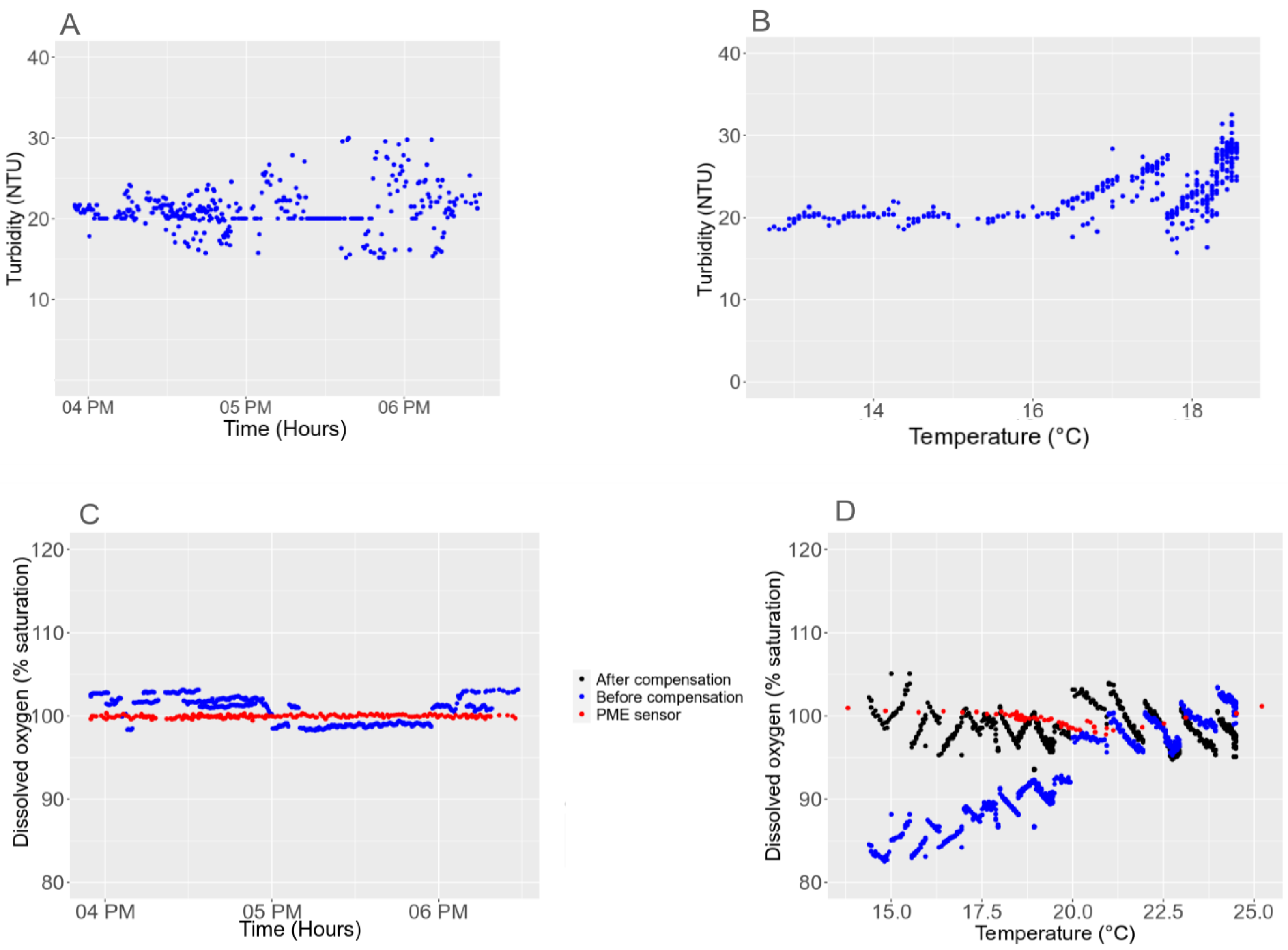
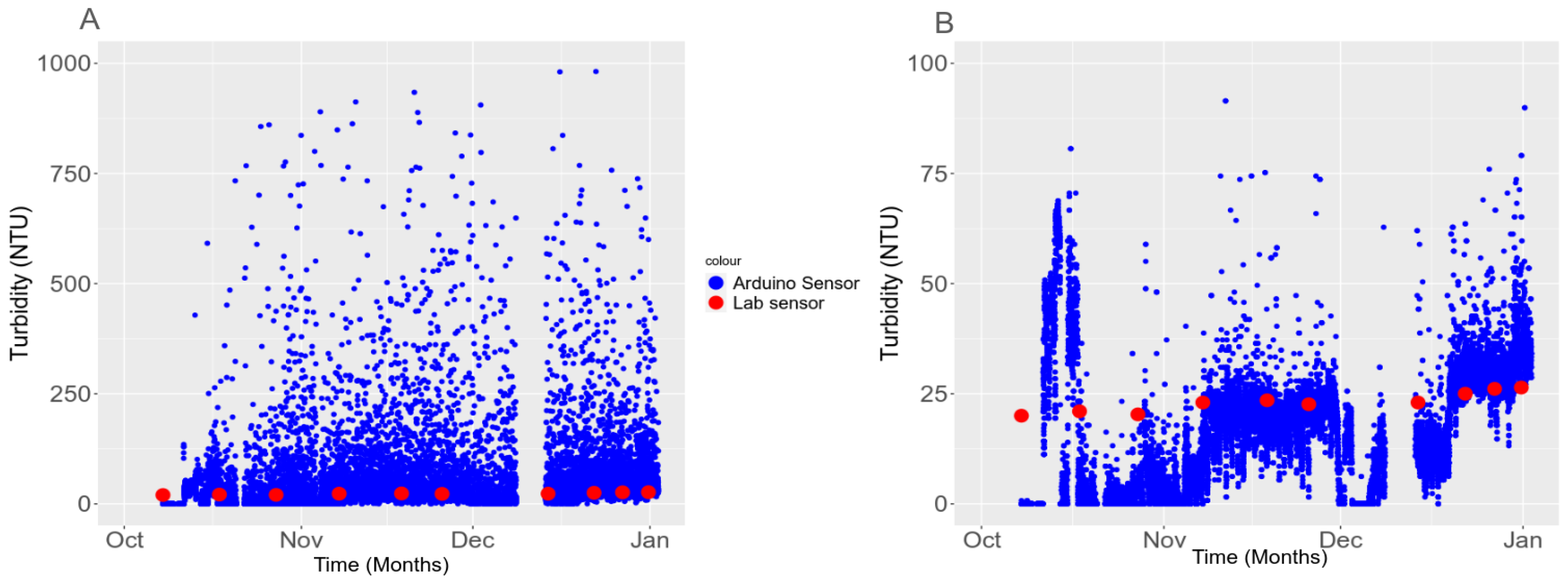
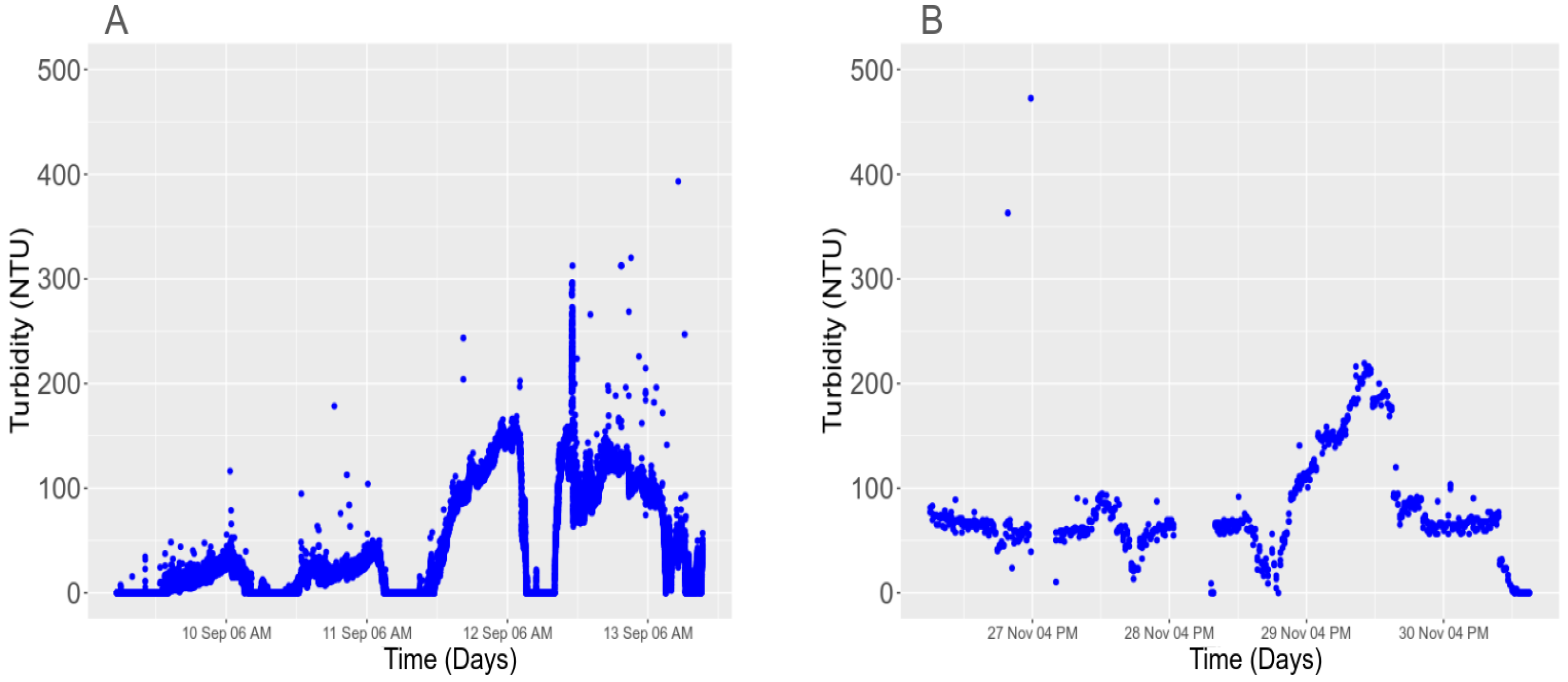
3.5.1. Light Interference with the Turbidity Sensor

The ambient infrared radiation interfered with the detection of the sensor infrared LED by the infrared photo transistor. This resulted in a daily oscillation of the turbidity readings, with a peak in the late afternoon and evening (Figure 8A). Trevathan et al. [39] also identified a degree of ambient infrared interference during the daytime using the same sensor. To avoid light interference from external light, the sensor should be shaded by a cover, an opaque box or a tubing, with the bottom open to allow water to circulate freely. Half of the bottom of the sensor with the infrared LED and the infrared phototransistor is not in the opaque box. This allows water to circulate between the two ends, without affecting the results obtained. We partly solved this light interference problem by shading the sensor using an opaque shell held with a weight above the sensor submerged in the water (Figure 8B). However, some variations were still present (Figure 8B), probably due to the inherent instability of this sensor and due to the indirect refracted light penetrating the water [39].

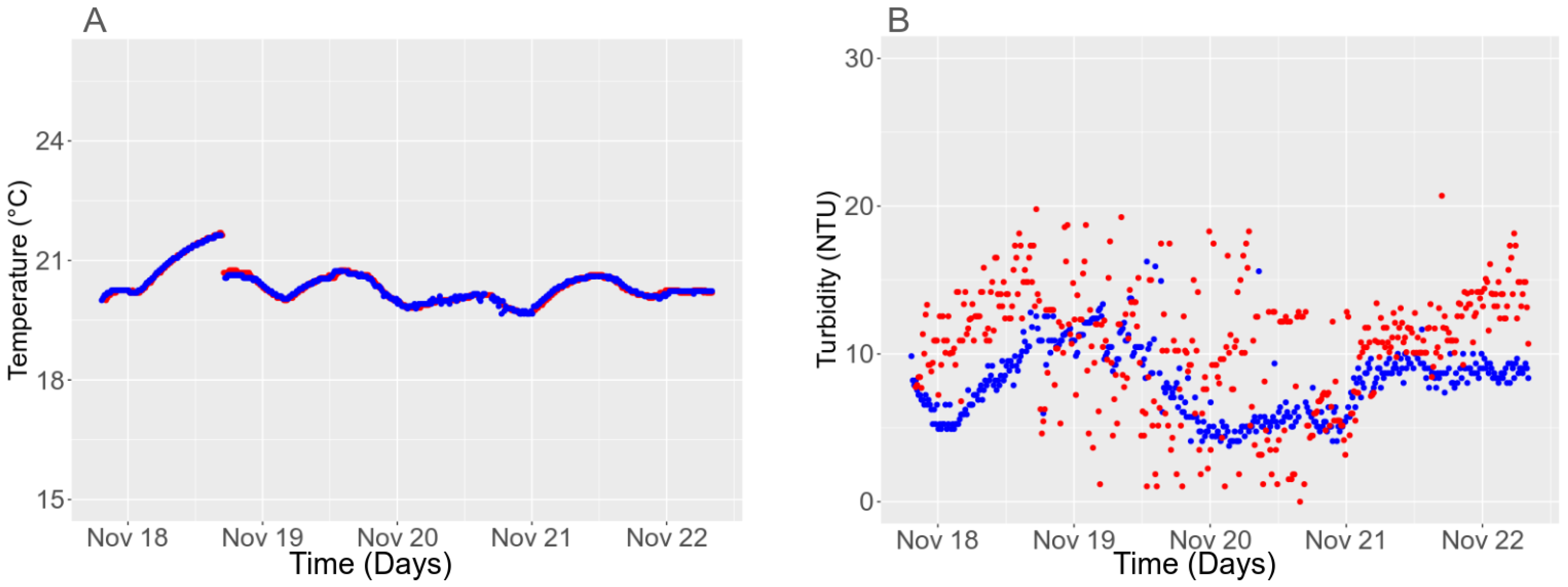
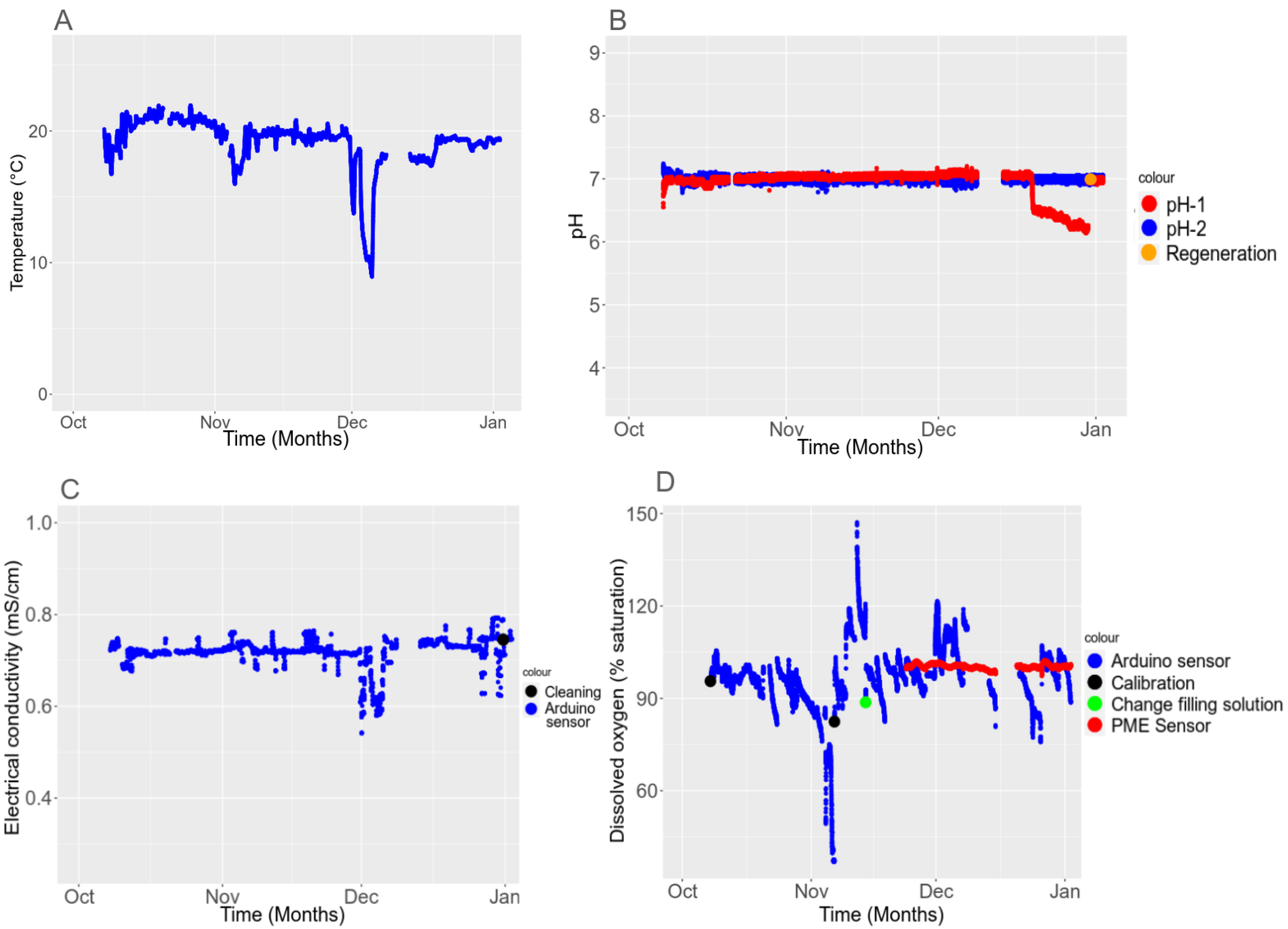
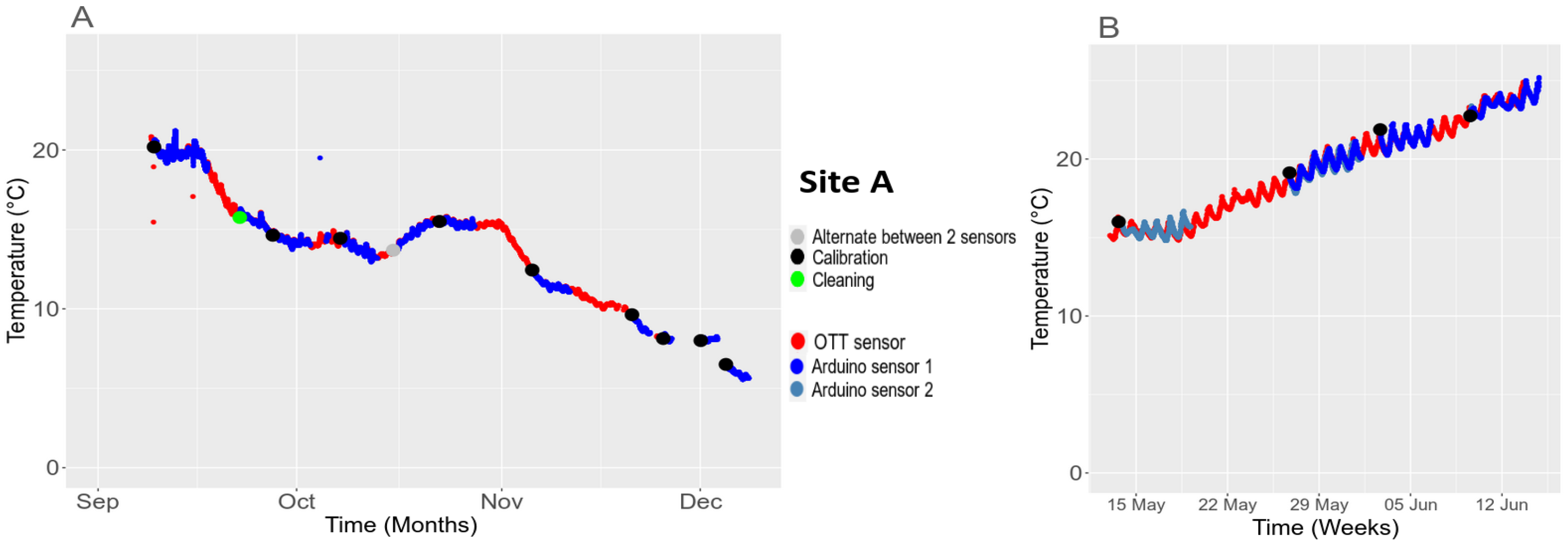
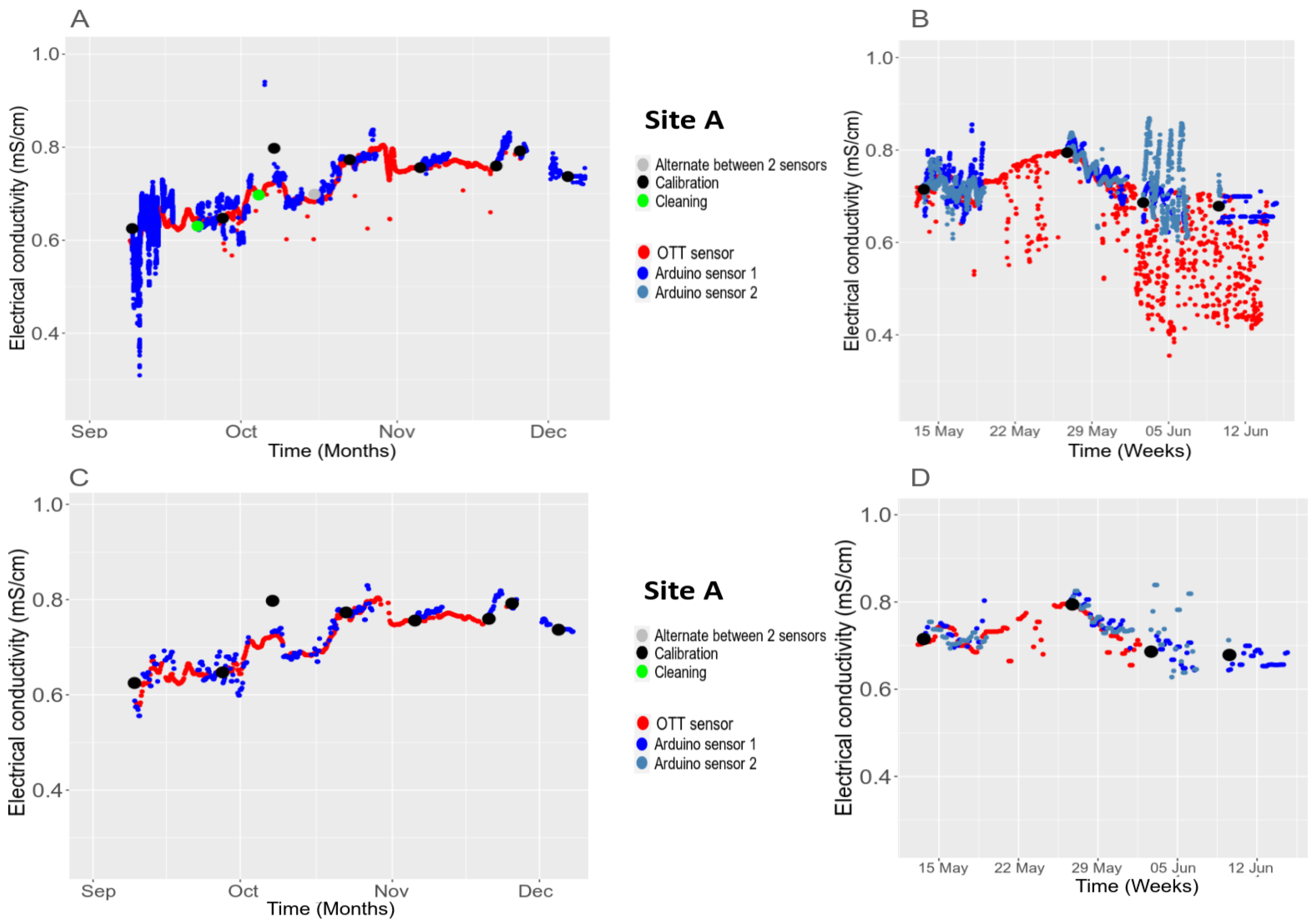
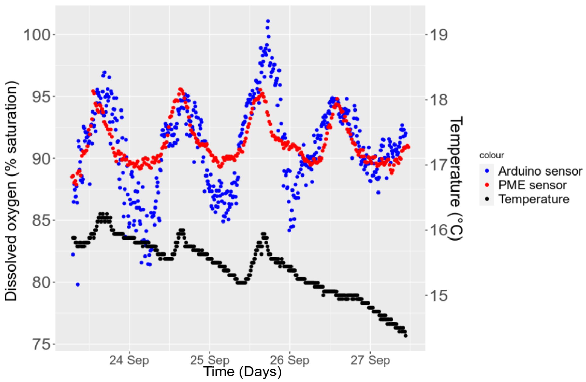
3.5.2. Temporal Stability in the Field

Although calibration with standard solutions is crucial to improve the accuracy of sensors, it is not sufficient. It is also essential to compare the results obtained from low-cost sensors with those of reference devices, such as high-resolution sensors, to ensure their validity [17].

To provide reliable data, the frequency of data acquisition should be selected to compromise between noise minimization and time resolution. During the first week of monitoring at La Villette, the time interval of 10 sec was too short and produced noised time series (Figure A6). Later, a setup of three measurements with 10-s intervals every 20 min helped in optimizing the data quality for the remaining monitoring period (Figure A6). The mean standard deviation between the three measurements was low for the temperature sensor (0.010 ± 0.004 °C), the 2 pH meters (0.028 ± 0.012 for pH-1 and 0.010 ± 0.007 for pH-2) and for the conductivity sensor (0.004 ± 0.001 $\mathrm{mS}·{\mathrm{cm}}^{-1}$). However, the difference between the repeat measurements of the turbidity sensor was high (42.4 ± 43.9 NTU), indicating low repeatability.

As already observed in the laboratory, the two units of the temperature sensor were highly reliable and accurate. The readings of the Arduino sensor were similar to the readings of the OTT sensor at both sites (A and B) (Figure 9 and Figure A8A). Similarly, Méndez-Barroso et al. [61] obtained very good performance results of the DS18b20 temperature sensor.

Field campaigns also confirmed that the pH-1 sensor, although reliable enough to enable monitoring, was less accurate and stable than the pH-2 meter (Figure A6). The standard deviation for the pH-1 meter was 0.14 (unit 1) and 0.33 (unit 2), whereas for the pH-2 meter, the deviation was slightly lower, at 0.10 and 0.22 for each unit, respectively. The OTT sensor was the most reliable, with a standard deviation of 0.09. Indeed, Demetillo et al. [71] also identified an average error of 0.18 for Atlas scientific sensors (which are slightly more costly than the pH-1 sensor) during a two-week test. This indicates the need to find the right balance between the cost and the accuracy of the sensor, which will depend on its intended use.

The Arduino conductivity sensors displayed a similar trend compared with the OTT sensors at both sites (Figure 10 and Figure A8B), although in May and June, few measurement errors could be observed due to soiling. During the spring and summer, regular maintenance is required due to biofouling as is visible for both the Arduino and the OTT sensors (Figure 10B). Data post-treatment (averaging over 4 h and removal of the outliers with ARIMA model) helped in providing time series of sufficient quality. Overall, the data obtained from the Arduino sensors agreed well with the OTT sensors, indicating that the low-cost sensors were effective in providing usable data. However, for setting an IoT of low-cost sensors, it should be kept in mind that the reproducibility of the two units of Arduino conductivity sensors was sometimes low (standard deviation of 0.17 mS·cm⁻¹ and 0.02 mS·cm⁻¹, respectively). It should not be forgotten that this sensor has low accuracy (factory certificate) since it is more suitable for monitoring water quality in mariculture [30]. Some other sensors are more accurate and more suitable for freshwater water; however, they are three times more expensive. For instance, the SEN0451 sensor from DFRobot displays an accuracy of 0.1 mS·cm⁻¹ [11,17,72].

Concerning the turbidity sensor, the readings were highly noised due to the instability of the sensor and light interference (Figure A7). Hacker et al. [23] tested for a month the same turbidity sensor and also identified an instability in the measurement. As noted by Hong et al. [19], the cable being too short, the sensor floats at the surface, leading to light interference. Fouling, as indicated by the gradual increase in NTU values (Figure A7B), triggered the requirement for regular maintenance.

Finally, the dissolved oxygen was measured over a few days, both by the Arduino sensor and the PME sensor at site B (Figure 11). The two sensors displayed similar trends, although the variation deviation was slightly greater for the Arduino sensor compared to the PME sensor (respectively 3.56% and 1.80%). Huan et al. [18] designed a low-cost dissolved oxygen sensor, which displayed an average error of 2.47%. Using this sensor, they also observed daily oscillations like we did, with peaks in the afternoon when the temperature increased. To demonstrate that low-cost sensors operate properly on site and to help in establishing their accuracy and reliability, long-term exposure in the field is a recommended procedure [17]. The low-cost temperature sensor was highly reliable, while the pH, conductivity and dissolved oxygen sensors gave relatively satisfactory results. Over time, small measurement errors tended to appear. This phenomenon was more pronounced for the Arduino sensors than for the OTT sensors. Similarly, other sensors from DFRobot or Atlas Scientific showed good stability and effectiveness with small measurement errors [17,18,71]. Considering the cost of the sensors tested in our study and their relatively low margin of error, their utilization for continuous measurement in the field was validated, given regular maintenance to ensure the reliability of the results. The results we obtained indicate that weekly cleaning and calibration of the Arduino sensors are necessary for some parameters. The labor cost associated with the weekly maintenance is hard to quantify since it depends on a variety of factors, such as the installation time, the number of sensors, and also the sites.

After each calibration, we recommend letting the sensors stabilize for a few hours in the standard solution before installation in the field. Finally, the turbidity sensor does not seem suitable for the continuous monitoring of fresh waters. In environmental conditions, the turbidity sensor quickly becomes soiled by biofilm, and the slightest particle or element that passes through, such as a leaf, may cause a variation in the readings. Trevathon et al. [39] also identified a fast negative impact of fouling (less then 48 h) on signal transmission. Zhu et al. [11] showed that even with other brands (TSD-10 and TSW-10 from Amphenol), the reproducibility appears rather poor for these low-cost turbidity sensors since they are all built on the same principle. The turbidity sensor should potentially be more suitable for detecting particular events with significantly high turbidity levels, such as wastewater [35,39]. The error rate decreased with increasing turbidity [11]. This rate was higher for turbidity levels above 100 NTU [35,73].

Based on this sensing device performance, we propose a framework to verify the reliability and stability and to identify necessary maintenance measurement intervals for each of the sensors (Figure 12). This framework can be generalized to all types of sensors other than those presented in this study so that they can be verified before installation and data processing. A more detailed synopsis of the framework is presented in Figure A10.

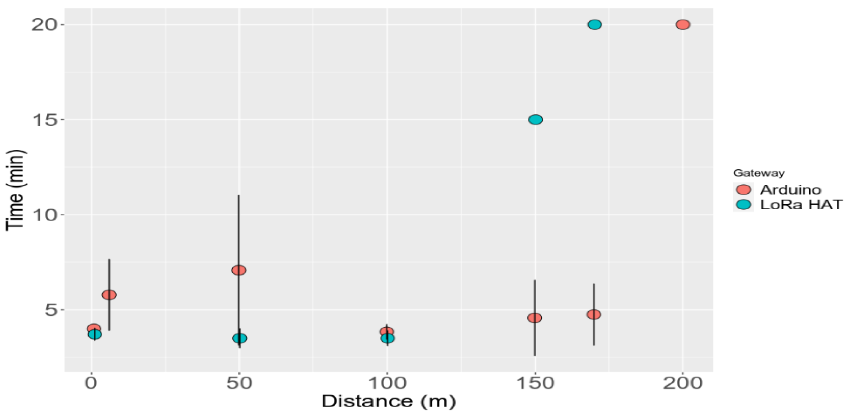
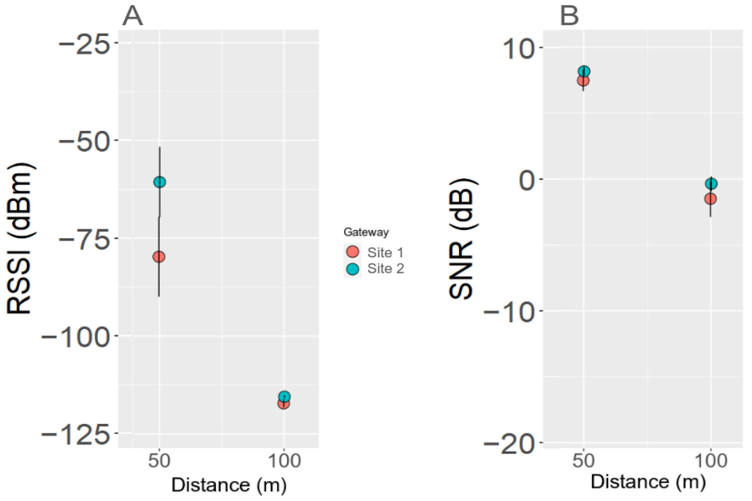
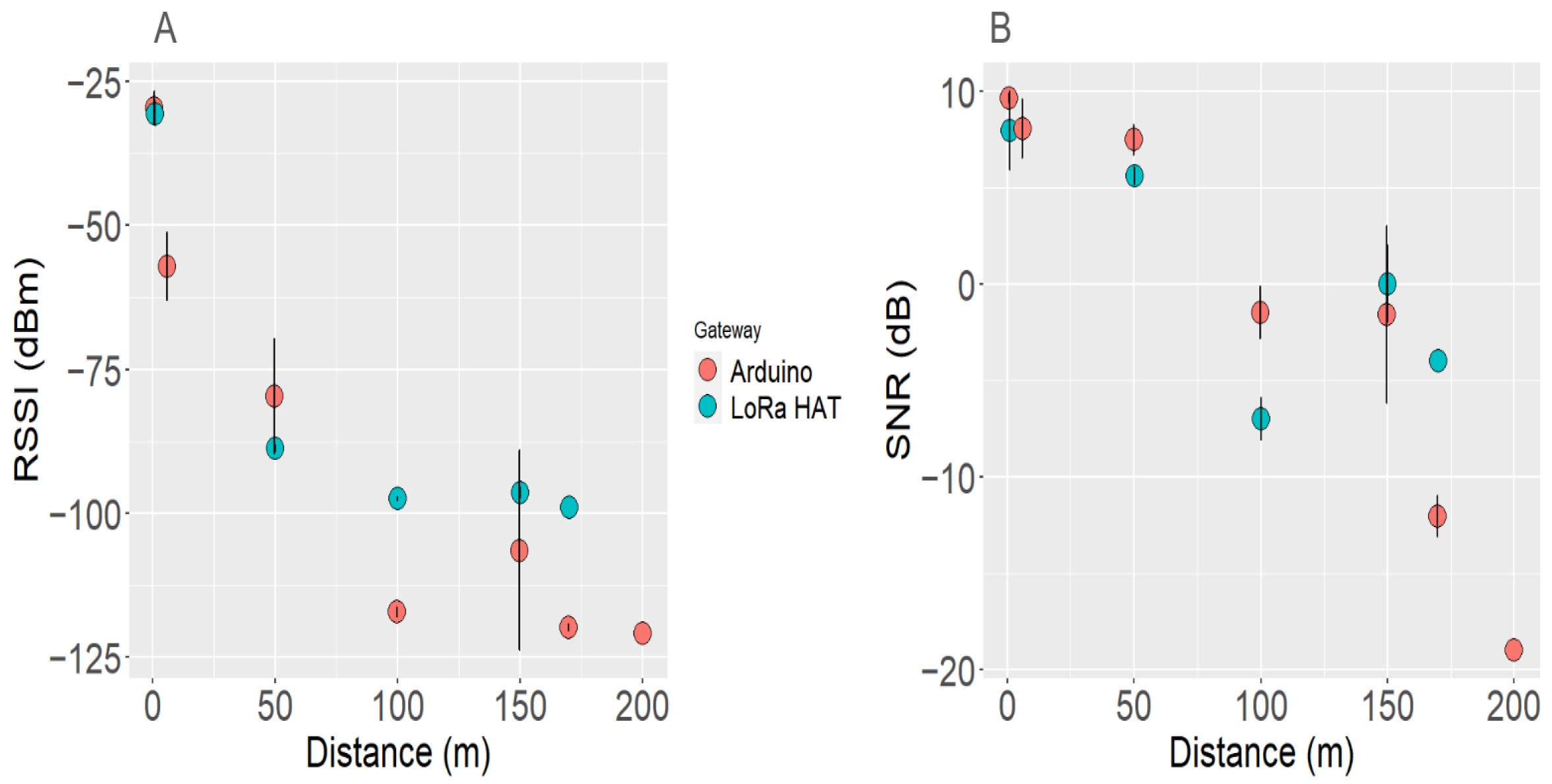
3.6. LoRa Gateway Performance

Long-range wide-area networks (LoRaWANs) were recently introduced as a promising low-power technology for several IoT applications, including networks to monitor water quality [13,74]. We analyzed the performance of two different LoRa gateways (a LoRa Arduino Pro gateway and a LoRa HAT gateway) in their ability to retrieve data from the end node device and to send them to the server without data corruption and loss. Both gateways were first tested in a dense urban area (Campus of Vitry, France). The maximum distance at which the node managed to send data was 200 m for the LoRa Arduino Pro gateway and 170 m for the LoRa HAT gateway, which is far below the potential distance announced by the manufacturer for the Arduino gateway (Figure 13).

Sendra et al. [75] similarly identified a maximum distance of 150 m with the same LoRa HAT gateway we used. Interference and path loss can occur due to structural obstacles, such as glass, metallic surfaces or walls, and due to the interference of other electronic components [47,75,76]. As a consequence, the signal propagation is obstructed, resulting in deterioration of the SNR and reduction in the RSSI levels with the increasing distance. After 100 m, we observed a rapid decline in the signal quality (RSSI levels) of both gateways, in the zone with the most obstacles. In the zone with fewer obstacles, the quality remained relatively unchanged between 100 and 200 m. Under 100 m, the LoRa HAT gateway exhibited better performance than the Arduino gateway, while it was the opposite between 100 and 200 m (Figure 13). Using a gateway combining the sx1278 (433 MHz) and ESP8266 modules, Zourmand et al. [76] also found that the quality signal decreased above 120 m from the gateway as indicated by the negative SNR (below the noise floor).

We also assessed the performance of the LoRa gateways with the time interval between the reception of two successive data (Figure A11). Up to 100 m, the interval between two measurements was short 5.25 ± 5.20 min for both gateways, though the LoRa HAT gateway displayed a better signal quality. Above 150 m, the time interval increased beyond 15 min for the LoRa HAT gateway, and over 20 min above 200 m for the LoRa Arduino gateway. However, even with a longer time reception, the quality and quantity of the data were still integral without any loss or degradation of the data collected. Beyond this distance limit, no data were received by the LoRa gateways.

The effect of the environment on the signal quality was tested with the LoRa Arduino gateway positioned in two different sites at a distance of 50 and 100 m. The first site was densely built, while the second site (residential area at Vitry, France) presented fewer buildings, and therefore fewer obstacles. Figure A12A,B show that for site 2, the signal quality was slightly better with higher RSSI at 50 m. However, there was no significant difference between the two sites (Wilcoxon test, p = 0.25, n = 72). This result is not surprising since coverage is usually much lower in urban areas than in open land such as rural areas, reaching up to several kilometers for the latter [77].

4. Conclusions

Our study demonstrated the suitability of the Arduino sensors (except the turbidity sensor) for monitoring water quality. In particular, the low-cost temperature sensor performed very well, as well as the two pH sensors, showing good repeatability and stability in the laboratory and in the field. However the pH-1 meter requires monthly maintenance, including regeneration of the sensor to remove any residue on the electrode. The low-cost conductivity sensor gave more variable results with lower accuracy. Similarly, the dissolved oxygen sensor was satisfying in terms of data acquisition and in terms of required maintenance. The filling solution should be changed every month and the membrane every 6 months (depending on frequency of use). The turbidity sensor is not recommended since it is too unstable and sensitive to external light. For a reliable low-cost sensing device, a balance has to be struck between cost and sensor reliability, depending on the sensor’s intended use.

A framework was then proposed to help characterizing and validating the sensing devices. This flexible framework makes it possible to integrate various sensors, to add or replace sensors as required, and to create a variety of devices to meet different measurement objectives and different water matrices. Finally, with a view to having a network of monitoring system, we tested two LoRa communication modules (LoRa HAT gateway and the LoRa Arduino pro gateway). Both performed well, with maximum communication distances, respectively, of 170 m and 200 m.

This low-cost monitoring device will be used in networks for the continuous acquisition of water quality data in a river. The provision of a dense multiprobes network integrated into an IoT system would enable real-time monitoring with greater precision due to the multitude of sensors. Coupling with a real-time anomaly detection system, like a nonlinear cooperative control algorithm based on game theory [78], would help in improving the continuous monitoring of surface water and reducing maintenance costs. Further studies are required to verify this hypothesis. The data collected with the devices will also feed machine learning models to predict the water quality and set up an alert system for urban bathing sites. It will also help with rationalizing the sampling strategy during the bathing season to measure bacterial indicators of fecal pollution. These combined approaches will improve sensor performance, reduce cost, and accelerate decision-making processes.

References

1. Bunsen, J.; Berger, M.; Finkbeiner, M. Planetary boundaries for water—A review. Ecol. Indic. 2021, 121, 107022. [Google Scholar] [CrossRef]
2. Whelan, M.J.; Linstead, C.; Worrall, F.; Ormerod, S.J.; Durance, I.; Johnson, A.C.; Johnson, D.; Owen, M.; Wiik, E.; Howden, N.J.; et al. Is water quality in British rivers “better than at any time since the end of the Industrial Revolution”? Sci. Total Environ. 2022, 843, 157014. [Google Scholar] [CrossRef]
3. Sutadian, A.D.; Muttil, N.; Yilmaz, A.G.; Perera, B. Development of river water quality indices—A review. Environ. Monit. Assess. 2016, 188, 58. [Google Scholar] [CrossRef]
4. Carvalho, D.V.; Pereira, E.M.; Cardoso, J.S. Machine learning interpretability: A survey on methods and metrics. Electronics 2019, 8, 832. [Google Scholar] [CrossRef]
5. Whelan, M.; Ramos, A.; Villa, R.; Guymer, I.; Jefferson, B.; Rayner, M. A new conceptual model of pesticide transfers from agricultural land to surface waters with a specific focus on metaldehyde. Environ. Sci. Process. Impacts 2020, 22, 956–972. [Google Scholar] [CrossRef]
6. WHO. World Health Organization. 2018. Available online: https://www.who.int/docs/default-source/wash-documents/who-recommendations-on-ec-bwd-august-2018.pdf (accessed on 16 July 2021).
7. Mouchel, J.M.; Lucas, F.S.; Moulin, L.; Wurtzer, S.; Euzen, A.; Haghe, J.P.; Rocher, V.; Azimi, S.; Servais, P. Bathing activities and microbiological river water quality in the Paris area: A long-term perspective. Seine River Basin Handb. Environ. Chem. 2020, 90, 323–354. [Google Scholar]
8. Yaroshenko, I.; Kirsanov, D.; Marjanovic, M.; Lieberzeit, P.A.; Korostynska, O.; Mason, A.; Frau, I.; Legin, A. Real-time water quality monitoring with chemical sensors. Sensors 2020, 20, 3432. [Google Scholar] [CrossRef]
9. Farouk, M.I.H.Z.; Latip, M.F.A.; Jamil, Z. Integrated water quality monitoring system and iot technology for surface water monitoring. AIP Conf. Proc. 2022, 2532, 050002. [Google Scholar]
10. McGrane, S.J. Impacts of urbanisation on hydrological and water quality dynamics, and urban water management: A review. Hydrol. Sci. J. 2016, 61, 2295–2311. [Google Scholar] [CrossRef]
11. Zhu, Q.; Cherqui, F.; Bertrand-Krajewski, J.L. End-user perspective of low-cost sensors for urban stormwater monitoring: A review. Water Sci. Technol. 2023, 87, 2648–2684. [Google Scholar] [CrossRef]
12. Kannel, P.R.; Lee, S.; Lee, Y.S.; Kanel, S.R.; Khan, S.P. Application of water quality indices and dissolved oxygen as indicators for river water classification and urban impact assessment. Environ. Monit. Assess. 2007, 132, 93–110. [Google Scholar] [CrossRef]
13. Wang, Z.A.; Moustahfid, H.; Mueller, A.V.; Michel, A.P.M.; Mowlem, M.; Glazer, B.T.; Mooney, T.A.; Michaels, W.; McQuillan, J.S.; Robidart, J.C.; et al. Advancing Observation of Ocean Biogeochemistry, Biology, and Ecosystems with Cost-Effective in situ Sensing Technologies. Front. Mar. Sci. 2019, 6, 519. [Google Scholar] [CrossRef]
14. Bogdan, R.; Paliuc, C.; Crisan-Vida, M.; Nimara, S.; Barmayoun, D. Low-Cost Internet-of-Things Water-Quality Monitoring System for Rural Areas. Sensors 2023, 23, 3919. [Google Scholar] [CrossRef]
15. Wuijts, S.; Friederichs, L.; Hin, J.A.; Schets, F.M.; Van Rijswick, H.F.; Driessen, P.P. Governance conditions to overcome the challenges of realizing safe urban bathing water sites. Int. J. Water Resour. Dev. 2022, 38, 554–578. [Google Scholar] [CrossRef]
16. Wuijts, S.; De Vries, M.; Zijlema, W.; Hin, J.; Elliott, L.R.; Dirven-van Breemen, L.; Scoccimarro, E.; de Roda Husman, A.M.; Külvik, M.; Frydas, I.S.; et al. The health potential of urban water: Future scenarios on local risks and opportunities. Cities 2022, 125, 103639. [Google Scholar] [CrossRef]
17. de Camargo, E.T.; Spanhol, F.A.; Slongo, J.S.; da Silva, M.V.R.; Pazinato, J.; de Lima Lobo, A.V.; Coutinho, F.R.; Pfrimer, F.W.D.; Lindino, C.A.; Oyamada, M.S.; et al. Low-Cost Water Quality Sensors for IoT: A Systematic Review. Sensors 2023, 23, 4424. [Google Scholar] [CrossRef]
18. Huan, J.; Li, H.; Wu, F.; Cao, W. Design of water quality monitoring system for aquaculture ponds based on NB-IoT. Aquac. Eng. 2020, 90, 102088. [Google Scholar] [CrossRef]
19. Hong, W.J.; Shamsuddin, N.; Abas, E.; Apong, R.A.; Masri, Z.; Suhaimi, H.; Gödeke, S.H.; Noh, M.N.A. Water quality monitoring with arduino based sensors. Environments 2021, 8, 6. [Google Scholar] [CrossRef]
20. Gowri, D.; Prasad, S.S.; Kiran, O.; Mysaiah, M.M. Water quality level monitoring system using arduino. J. Eng. Sci. 2023, 14, 226–229. [Google Scholar]
21. Sekhar, K.C.; Venkatesh, B.; Reddy, K.S.; Giridhar, G.; Nithin, K.; Eshwar, K. IoT-based Realtime Water Quality Management System using Arduino Microcontroller. Turk. J. Comput. Math. Educ. (TURCOMAT) 2023, 14, 783–792. [Google Scholar]
22. Cheniti, M.; Abdesslam, B.; Kaouthar, R. An Arduino-Based Water Quality Monitoring System Using pH, Temperature, Turbidity, and TDS Sensors. Available online: https://www.researchgate.net/profile/Cheniti-Mohamed/publication/371608557_An_Arduino-based_Water_Quality_Monitoring_System_using_pH_Temperature_Turbidity_and_TDS_Sensors/links/648c186bc41fb852dd0a0b70/An-Arduino-based-Water-Quality-Monitoring-System-using-pH-Temperature-Turbidity-and-TDS-Sensors.pdf (accessed on 13 December 2023).
23. Hacker, J. Assessing the Ability of Arduino-Based Sensor Systems to Monitor Changes in Water Quality. Ph.D. Thesis, Georgia Southern University, Statesboro, GA, USA, 2023. [Google Scholar]
24. Trevathan, J.; Schmidtke, S.; Read, W.; Sharp, T.; Sattar, A. An IoT general-purpose sensor board for enabling remote aquatic environmental monitoring. Internet Things 2021, 16, 100429. [Google Scholar] [CrossRef]
25. Wong, Y.J.; Nakayama, R.; Shimizu, Y.; Kamiya, A.; Shen, S.; Muhammad Rashid, I.Z.; Nik Sulaiman, N.M. Toward industrial revolution 4.0: Development, validation, and application of 3D-printed IoT-based water quality monitoring system. J. Clean. Prod. 2021, 324, 129230. [Google Scholar] [CrossRef]
26. Abotaleb, M. Authenticated WiFi-Based Wireless Data Transmission from Multiple Sensors through a Laboratory Stand Based on Collaboration between ATMEGA2560 and ESP32 Microcontrollers. Sci. J. Gdyn. Marit. Univ. 2023, 27–41. [Google Scholar] [CrossRef]
27. Randika, M.; Amarasooriya, A.; Weragoda, S. Development of an arduino-based low-cost turbidity and electric conductivity meter for wastewater characterization. Larhyss J. 2022, 51, 115–127. [Google Scholar]
28. Dfrobot. Available online: https://www.dfrobot.com/ (accessed on 1 September 2023).
29. I2C ADS1115 16-Bit ADC Module. Available online: https://www.dfrobot.com/product-1730.html (accessed on 25 November 2023).
30. Analog Electrical Conductivity Meter V2. Available online: https://wiki.dfrobot.com/Gravity__Analog_Electrical_Conductivity_Sensor___Meter_V2__K=1__SKU_DFR0300 (accessed on 11 November 2023).
31. Hem, J.D. Study and Interpretation of the Chemical Characteristics of Natural Water; Department of the Interior, US Geological Survey: Reston, VA, USA, 1985; Volume 2254.
32. DS18B20 Arduino Temperature Sensor. Available online: https://wiki.dfrobot.com/Waterproof_DS18B20_Digital_Temperature_Sensor__SKU_DFR0198_ (accessed on 25 November 2023).
33. pH Meter V2. Available online: https://wiki.dfrobot.com/Gravity__Analog_pH_Sensor_Meter_Kit_V2_SKU_SEN0161-V2 (accessed on 24 November 2023).
34. pH Meter 2 V2. Available online: https://wiki.dfrobot.com/Analog_pH_Meter_Pro_SKU_SEN0169 (accessed on 24 November 2023).
35. Hakim, W.; Hasanah, L.; Mulyanti, B.; Aminudin, A. Characterization of turbidity water sensor SEN0189 on the changes of total suspended solids in the water. J. Phys. Conf. Ser. 2019, 1280, 022064. [Google Scholar] [CrossRef]
36. For Arduino. A.T.S. Available online: https://www.dfrobot.com/product-1394.html (accessed on 15 November 2023).
37. Analog Disslved Oxygen Sensor. Available online: https://wiki.dfrobot.com/Gravity__Analog_Dissolved_Oxygen_Sensor_SKU_SEN0237 (accessed on 20 November 2023).
38. Villeneuve, V.; Légaré, S.; Painchaud, J.; Vincent, W. Dynamique et modélisation de l’oxygène dissous en rivière. Rev. Des. Sci. De L’eau 2006, 19, 259–274. [Google Scholar] [CrossRef]
39. Trevathan, J.; Read, W.; Schmidtke, S. Towards the Development of an Affordable and Practical Light Attenuation Turbidity Sensor for Remote Near Real-Time Aquatic Monitoring. Sensors 2020, 20, 1993. [Google Scholar] [CrossRef]
40. Arduino Pro Gateway. Available online: https://www.cascoantiguopro.com/fr/oceanographie/capteurs-oceanographie/minidot-logger.html (accessed on 3 May 2023).
41. Hydrolab DS5X, D. M.W.Q.M. Available online: https://www.ott.com/download/user-manual-hydrolab-ds5x-ds5-and-ms5-water-quality-multiprobes-1/ (accessed on 4 January 2024).
42. D.L.S. Available online: https://wiki1.dragino.com/index.php/Lora_Shield (accessed on 4 November 2023).
43. R.P.L.H. Available online: https://fr.farnell.com/seeed-studio/113990254/gps-lora-hat-for-raspberry-pi/dp/3498581?gad_source=5&cjevent=6c2f6bd47f0811ee816c1cda0a18ba74&cjdata=MXxZfDB8WXww&CMP=AFC-CJ-FR-1765328&gross_price=true&source=CJ (accessed on 1 November 2023).
44. A.P.G.D. Available online: https://docs.arduino.cc/retired/kits/pro-gateway (accessed on 1 November 2023).
45. Tsanousa, A.; Xefteris, V.R.; Meditskos, G.; Vrochidis, S.; Kompatsiaris, I. Combining RSSI and Accelerometer Features for Room-Level Localization. Sensors 2021, 21, 2723. [Google Scholar] [CrossRef]
46. Audéoud, H.J.; Heusse, M.; Duda, A. Single reception estimation of wireless link quality. In Proceedings of the 2020 IEEE 31st Annual International Symposium on Personal, Indoor and Mobile Radio Communications, London, UK, 31 August–3 September 2020; IEEE: Piscataway, NJ, USA, 2020; pp. 1–7. [Google Scholar]
47. Guidara, A.; Fersi, G.; Jemaa, M.B.; Derbel, F. A new deep learning-based distance and position estimation model for range-based indoor localization systems. Ad Hoc Netw. 2021, 114, 102445. [Google Scholar] [CrossRef]
48. Guillot-Le Goff, A.; Angelotti, N.; Carmigniani, R.; Souza, G.C.; Saad, M.; Dubois, P.; Vinçon-Leite, B. Prévision de la qualité Microbiologique des Milieux Aquatiques: Modélisation Hydrodynamique Pour Anticiper des Épisodes de Contamination Microbiologique sur des Sites de Baignade Urbaine. In Proceedings of the Novatech 2023: 11e Conférence Internationale sur l’Eau dans la Ville; 2023. Available online: https://hal.science/hal-04176992/ (accessed on 5 December 2023).
49. Venelinov, T. Comparison of ISO 21748 and ISO 11352 standards for measurement uncertainty estimation in water analysis. Ovidius Univ. Ann. Ser. Civ. Eng. 2016, 18, 187–192. [Google Scholar]
50. Moyón Rivera, C.W.; Ordóñez Berrones, D.K. Construcción de un Prototipo de Red de Nodos Inteligentes Para Supervisar la Calidad y Niveles del Agua Potable en los Tanques de Reserva de EP-EMAPAR. Bachelor’s Thesis, Escuela Superior Politécnica de Chimborazo, Riobamba, Ecuador, 2019. [Google Scholar]
51. Saputra, R.E.; Irawan, B.; Nugraha, Y.E. System design and implementation automation system of expert system on hydroponics nutrients control using forward chaining method. In Proceedings of the 2017 IEEE Asia Pacific Conference on Wireless and Mobile (APWiMob), Bandung, Indonesia, 28–29 November 2017; IEEE: Piscataway, NJ, USA, 2017; pp. 41–46. [Google Scholar]
52. Rozaq, I.A.; Setyaningsih, N.Y.D.; Gunawan, B. Pengkondisian Sinyal Sensor Salinitas Dfr0300 Menggunakan Arduino Due. 2020. Available online: https://www.unisbank.ac.id/ojs/index.php/sendi_u/article/view/8022 (accessed on 10 April 2023).
53. Hayashi, M. Temperature-electrical conductivity relation of water for environmental monitoring and geophysical data inversion. Environ. Monit. Assess. 2004, 96, 119–128. [Google Scholar] [CrossRef]
54. Jeroschewski, P.; Zur Linden, D. A flow system for calibration of dissolved oxygen sensors. Fresenius’ J. Anal. Chem. 1997, 358, 677–682. [Google Scholar] [CrossRef]
55. Clesceri, L.S. Standard Methods for Examination of Water and Wastewater; American Public Health Association: Washington, DC, USA, 1998; Volume 9. [Google Scholar]
56. Keller, G.V.; Frank, C. Electrical Methods in Geophysical Prospecting; Pergamon Press: Oxford, UK, 1966. [Google Scholar]
57. Hitchman, M.L. Measurement of Dissolved Oxygen; Wiley: New York, NY, USA, 1978. [Google Scholar]
58. Boards. Available online: https://support.arduino.cc/hc/en-us/articles/360016076980-What-is-the-operating-temperature-range-for-Arduino-boards (accessed on 10 April 2023).
59. Alimorong, F.M.L.S.; Apacionado, H.A.D.; Villaverde, J.F. Arduino-based multiple aquatic parameter sensor device for evaluating pH, turbidity, conductivity and temperature. In Proceedings of the 2020 IEEE 12th International Conference on Humanoid, Nanotechnology, Information Technology, Communication and Control, Environment, and Management (HNICEM), Manila, Philippines, 3–7 December 2020; IEEE: Piscataway, NJ, USA, 2020; pp. 1–5. [Google Scholar]
60. Saha, S.; Rajib, R.H.; Kabir, S. IoT based automated fish farm aquaculture monitoring system. In Proceedings of the 2018 International Conference on Innovations in Science, Engineering and Technology (ICISET), Chittagong, Bangladesh, 27–28 October 2018; IEEE: Piscataway, NJ, USA, 2018; pp. 201–206. [Google Scholar]
61. Méndez-Barroso, L.; Rivas-Márquez, J.; Sosa-Tinoco, I.; Robles-Morúa, A. Design and implementation of a low-cost multiparameter probe to evaluate the temporal variations of water quality conditions on an estuarine lagoon system. Environ. Monit. Assess. 2020, 192, 710. [Google Scholar] [CrossRef]
62. Xu, S.; Lu, B.; Baldea, M.; Edgar, T.F.; Wojsznis, W.; Blevins, T.; Nixon, M. Data cleaning in the process industries. Rev. Chem. Eng. 2015, 31, 453–490. [Google Scholar] [CrossRef]
63. Le Deunf, J.; Debese, N.; Schmitt, T.; Billot, R. A review of data cleaning approaches in a hydrographic framework with a focus on bathymetric multibeam echosounder datasets. Geosciences 2020, 10, 254. [Google Scholar] [CrossRef]
64. Wang, X.; Wang, C. Time series data cleaning: A survey. IEEE Access 2019, 8, 1866–1881. [Google Scholar] [CrossRef]
65. Sedaghat, L.; Hersey, J.; McGuire, M.P. Detecting spatio-temporal outliers in crowdsourced bathymetry data. In Proceedings of the Second ACM SIGSPATIAL International Workshop on Crowdsourced and Volunteered Geographic Information, Orlando, FL, USA, 5 November 2013; pp. 55–62. [Google Scholar]
66. Yang, J.; Rahardja, S.; Fränti, P. Mean-shift outlier detection and filtering. Pattern Recognit. 2021, 115, 107874. [Google Scholar] [CrossRef]
67. Bianco, A.M.; Garcia Ben, M.; Martinez, E.; Yohai, V.J. Outlier detection in regression models with arima errors using robust estimates. J. Forecast. 2001, 20, 565–579. [Google Scholar] [CrossRef]
68. Liu, H.; Shah, S.; Jiang, W. On-line outlier detection and data cleaning. Comput. Chem. Eng. 2004, 28, 1635–1647. [Google Scholar] [CrossRef]
69. Shi, M.; Ma, J.; Zhang, K. The Impact of Water Temperature on In-Line Turbidity Detection. Water 2022, 14, 3720. [Google Scholar] [CrossRef]
70. Sensor. Available online: https://www.hemmis.com/docs/hydrolab/MS5_DS5_DS5X_low_F.pdf (accessed on 5 January 2024).
71. Demetillo, A.T.; Japitana, M.V.; Taboada, E.B. A system for monitoring water quality in a large aquatic area using wireless sensor network technology. Sustain. Environ. Res. 2019, 29, 12. [Google Scholar] [CrossRef]
72. Analog Electrical Conductivity Meter Pro. Available online: https://wiki.dfrobot.com/SKU_SEN0451_Gravity_Analog_Electrical_Conductivity_Sensor_PRO_K_1 (accessed on 24 May 2024).
73. Gusri, A.J.; Harmadi, H. Rancang Bangun Alat Penguras Air pada Wadah Penampungan Berbasis Turbidity Sensor SEN0189. J. Fis. Unand 2021, 10, 330–336. [Google Scholar] [CrossRef]
74. Jiang, J.; Tang, S.; Han, D.; Fu, G.; Solomatine, D.; Zheng, Y. A comprehensive review on the design and optimization of surface water quality monitoring networks. Environ. Model. Softw. Environ. Data News 2020, 132, 104792. [Google Scholar] [CrossRef]
75. Sendra, S.; Parra, L.; Jimenez, J.M.; Garcia, L.; Lloret, J. LoRa-based network for water quality monitoring in coastal areas. Mob. Netw. Appl. 2023, 28, 65–81. [Google Scholar] [CrossRef]
76. Zourmand, A.; Hing, A.L.K.; Hung, C.W.; AbdulRehman, M. Internet of things (IoT) using LoRa technology. In Proceedings of the 2019 IEEE International Conference on Automatic Control and Intelligent Systems (I2CACIS), Selangor, Malaysia, 29 June 2019; IEEE: Piscataway, NJ, USA, 2019; pp. 324–330. [Google Scholar]
77. Petrariu, A.I.; Lavric, A.; Coca, E. Lorawan gateway: Design, implementation and testing in real environment. In Proceedings of the 2019 IEEE 25th International Symposium for Design and Technology in Electronic Packaging (SIITME), Cluj-Napoca, Romania, 23–26 October 2019; IEEE: Piscataway, NJ, USA, 2019; pp. 49–53. [Google Scholar]
78. Casado-Vara, R.; Prieto-Castrillo, F.; Corchado, J.M. A game theory approach for cooperative control to improve data quality and false data detection in WSN. Int. J. Robust Nonlinear Control 2018, 28, 5087–5102. [Google Scholar] [CrossRef]
Figure 1. Synoptic view of the low-cost system for water quality monitoring in real time.
Water 16 01708 g001
Figure 2. Installation sites (A,B) and parameters measured by each type of sensor (source: Google Maps).
Water 16 01708 g002
Figure 3. Hardware components involved in the field experiment: 1: temperature, 2: turbidity, 3: conductivity, 4: pH-1, 5: pH-2, 6: dissolved oxygen, A: LoRa HAT gateway, B: LoRa Arduino Pro gateway.
Water 16 01708 g003
Figure 4. Comparison of two unit sensors placed simultaneously in the same solution. In blue unit 1, and in red unit 2. (A) Temperature, (B) turbidity.
Water 16 01708 g004
Figure 5. Temperature effect on the turbidity and dissolved oxygen. (AC) Fixed temperature analysis, (B) turbidity measurement at different temperatures, (D) Dissolved oxygen before compensation in blue, after compensation in black and the PME sensor in red.
Water 16 01708 g005
Figure 6. Long-term turbidity analysis. The blue dots correspond to measurements taken by the sensors and the red dots to measurements taken by the laboratory turbidimeter. (A) Raw data, and (B) after removal of outlier using ARIMA with a median filter (width of 5).
Water 16 01708 g006
Figure 7. Long-term stability of sensors reading standard solutions. (A) Temperature, (B) pH, (C) conductivity measurement cleaned with an ARIMA model and median filter (width of 11), and (D) dissolved oxygen measurement cleaned with an ARIMA model and median filter (width of 5).
Water 16 01708 g007
Figure 8. Effect of the ambient light on the reading of the turbidity sensor. (A) Before shading, and (B) after shading.
Water 16 01708 g008
Figure 9. Temperature analysis at Site A at Bassin de La Villette. Values from OTT sensors are displayed in red, Arduino sensors in blue. Black dots indicate that the sensor has been calibrated, green dots that it has been cleaned, and gray dots that the sensor has been replaced. Replacements were carried out by alternating the two units of the same sensor every week. (A) From early September 2022 to early January 2023, and (B) from May to June 2023.
Water 16 01708 g009
Figure 10. Conductivity measurement at site A at Bassin de la Villette. Values of the OTT sensors are displayed in red, and Arduino sensors in blue. Black dots indicate that the sensor has been calibrated, green dots that it has been cleaned, and gray dots that the unit has been replaced. Replacements were carried out by alternating the two units of the same sensor every week. (A) From early September 2022 to early January 2023, (B) from May to June 2023, and (C,D) data from (A,B) averaged over 4 h and cleaned by ARIMA.
Water 16 01708 g010
Figure 11. Dissolved oxygen measurements at site B at Bassin de la Villette. Values of the PME sensor are displayed in red, Arduino sensors in blue, and Arduino temperature sensors in black.
Water 16 01708 g011
Figure 12. Framework for testing the reliability of sensors.
Water 16 01708 g012
Figure 13. LoRa gateway performance. Arduino LoRa gateway in pink, LoRa HAT gateway in blue light. (A) Received signal strength indicator (RSSI), (B) Signal-to-Noise Ratio (SNR).
Water 16 01708 g013