Using MODFLOW to Model Riparian Wetland Shallow Groundwater and Nutrient Dynamics in an Appalachian Watershed

Abstract

Simulating shallow groundwater (SGW) flow dynamics and stream–SGW interactions using numerical modeling tools is necessary to develop a mechanistic understanding of water flow systems and improve confidence in water resource management practices. A three-dimensional (3D) SGW flow model was developed for a riparian wetland in a mixed forest and agricultural catchment in West Virginia (WV), Appalachia, USA, using a Modular 3D Groundwater Model (MODFLOW). The MODFLOW simulation was calibrated in steady (R² = 0.98, ME = −0.21, and RMSE = 0.77), transient state (R² = 0.97, ME = −0.41, and RMSE = 1.28) and validated (R² = 0.97, ME = −0.28, and RMSE = 1.05) using observed SGW levels from thirteen nested piezometers under steady and transient states. An experimental MT3D transport scenario was developed to show the lateral transport of NO₃-N from the aquifer to stream cells. Relatively stable SGW head distribution was observed. In the downstream reach, SGW discharge varied from 948 m³/day to 907 m³/day in 2020, with creek seepage ranging from 802 m³/day to 790 m³/day. Similarly, SGW input to the stream ranged from 891 m³/day to 978 m³/day, while creek seepage ranged from 796 m³/day to 800 m³/day in 2021. In upstream reaches, losing stream conditions were observed in January, June, and September 2020 and January to April 2021, while gaining stream conditions prevailed during other months. Thus, an approximately monthly alternating gaining–losing stream condition was observed in the upstream area. An experimental MT3D transport scenario resulted in an advection–dispersion scenario, showing a cumulative loss of 947 g of NO₃-N from SGW to the stream. Denitrification accounted for the cumulative loss of 1406 g of NO₃-N from SGW, surpassing 639 g of nitrate from the SGW to the stream during the study period. Additionally, particle tracking using MODPATH indicated a long residence time for SGW nutrients, affirming the efficiency of nitrogen transformation through denitrification. This study is among the first to simulate hydrologic and nutrient interactions in riparian wetlands of a mixed land use catchment in the Appalachian region of the northeastern United States. The results better inform water resource management decisions and modeling efforts in the Appalachian region and similar physiographic regions globally.

1. Introduction

Shallow groundwater (SGW) is generally defined as groundwater in aquifers less than six meters below the soil surface and is typically unrestricted by confining layers [1]. Due to proximity to the land surface, SGW is more sensitive to surface fluctuations and perturbations, such as precipitation, surface recharge rates, land use practices, and nutrient leaching [1,2,3,4]. Approximately half of the streams in the continental USA are estimated to include SGW flow processes, including discharge, contributing to streamflow [1]. As SGW discharges influence water quality and quantity in the stream network, effective watershed management requires a mechanistic understanding of SGW flow dynamics and related interactions with surface-receiving waters. For example, SGW can discharge to stream water (SW) if the SGW table is elevated relative to the stream stage (i.e., gaining stream) [5,6,7]. Conversely, if the SW level is higher than the SGW head, SW contributes to subsurface water volume and flow (i.e., losing stream) [6,7]. Generally, dynamic stream-SGW hydrologic connectivity is established in SGW discharge zones through advective water exchange [1]. Such mechanistic processes affect both environments’ nutrient transport dynamics, water quantity, and quality [1,6,8]. Therefore, understanding the relationship between SW and SGW flow regimes is vital to optimizing their conjunctive use [1,2,9,10].

Shallow groundwater–stream water hydrologic exchange processes greatly influence NO₃-N transport processes, a major nutrient affecting aquifer and stream water quality [11,12]. NO₃-N can be a concern in water resources due to its high solubility, susceptibility to leaching, and low sorption capacity. However, NO₃-N can undergo chemical reduction (i.e., denitrification) under anaerobic and redox conditions [13]. SGW tables in riparian wetlands primarily determine redox conditions and denitrification [14,15]. During high-precipitation events, N accumulated in wetland soil can leach to SGW, be delivered to the stream via SGW discharge, and increase the NO₃-N loading in SW [5,16,17]. For example, Kwon et al. [18] demonstrated that elevated SW nitrogen (N) concentrations were linked to SGW flow to the stream during gaining stream conditions. While studying nutrient loading in SGW, Ouyang et al. [17] observed that SGW discharge was the primary contributor of nitrate load in the Lower St. Johns River, Florida, suggesting that a seasonal SGW level change and higher SGW nitrate concentrations were the driving forces for NO₃-N loading in the stream. Ruiz et al. [19] supported this argument, emphasizing the role of SGW mixing with stream water in governing nutrient fate and transport. Previous studies clearly show the relevance of understanding SGW-SW processes to delineate NO₃-N transport pathways and dynamics [14,20].

Three-dimensional (3D) numerical simulation models are valuable tools to accurately quantify SW-SGW interaction and nutrient transport [21,22,23]. The Modular 3D Groundwater Model (MODFLOW) is an international standard for estimating groundwater flow [24,25]. For example, Colombo et al. [23] applied MODFLOW in the NW Milano Functional Urban Area to reconstruct the long-term GW flow trend (1980–2018) and suggested that nutrient transport pathways can be predicted as a transient GW flow variation function. The authors developed a predictive scenario using the MODFLOW- nutrient transport subroutine Model Transport Three-Dimensional Model Simulator (MT3DMS) [26] to simulate the potential evolution of contaminants in GW. Similarly, Chinnasamy and Hubbart [9] adapted MODFLOW-MT3DMS to simulate SW-SGW hydrologic and nutrient interaction in the Ozark border forest in the central USA. Karlovi’c et al. [21] used MODFLOW-MT3DMS to simulate steady-state GW flow and nitrate transport in the alluvial aquifer of the Varazdin region of NW Croatia. Additionally, the authors performed a scenario analysis to investigate the response of NO₃-N concentration in the aquifer based on a change in NO₃-N input from nonpoint sources. Their analysis indicated that NO₃-N attenuation in GW is low; reducing nitrate input from agricultural areas was necessary to reduce NO3-N loadings significantly. Rajaeian et al. [22] used MODFLOW-MT3DMS to observe the NO₃-N change in GW resources in Iran under different management scenarios and suggested that the artificial recharge of GW helped decrease NO₃-N concentrations. Previous studies clearly show the value of using numerical simulation models and nutrient transport scenario analysis to predict nutrient transport processes under different conditions to make better-informed management decisions.

Despite the progress of previous research regarding GW flow dynamics and SW-GW interactions using numerical models, there is a lack of such studies in the Appalachian region of the United States [27,28]. As water is a primary natural resource commodity of Appalachia, it is imperative to maintain the quality of surface and subsurface water [29]. Thus, the main aim of this research was to examine the SGW flow dynamics and SGW interaction with stream water in the riparian wetlands of a mixed land use watershed in the Appalachian region of West Virginia (WV), USA. Sub-objectives included (a) calibrating and validating the SGW flow model MODFLOW using observed SGW data from 13 piezometers in a steady and transient state, (b) performing an experimental scenario analysis of NO₃-N transport under advection, dispersion, and chemical reaction scenario using MT3D-USGS, and (c) quantifying the amount of NO₃-N loss due to SGW discharge to stream and due to denitrification. The results provide new information on water management strategies and science-based information about the SGW environment, SW-SGW mixing, and NO₃-N transport in riparian wetlands of mixed land use watersheds.

2. Materials and Methods

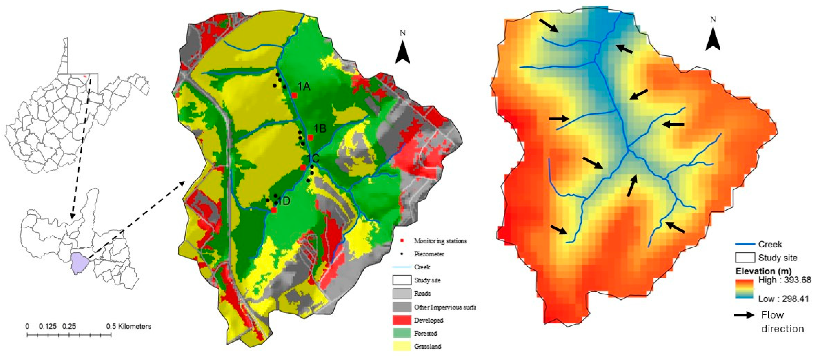
2.1. Study Area

The current research was conducted in periodically flooded riparian wetlands of a second-order reach in the mixed land use West Run Watershed (WRW) located in northeastern Morgantown, West Virginia (WV), USA (Figure 1). The study reach drains into the third-order West Run Creek, a Monongahela River tributary [30,31,32]. This study used a scale-nested and paired experimental design described in previous investigations [15,30,31,33,34,35]. The study reach was instrumented with four stream-stage monitoring sites designated 1A, 1B, 1C, and 1D, along with co-located piezometers (Figure 1). Site 1A had four co-located piezometers, and all other sites had three co-located piezometers, resulting in 13 total piezometers. The distances of piezometers from stream at sites 1A to 1D ranged from 16 m to 55 m, 18 m to 28 m, 24 m to 40 m, and 8 m to 43 m, respectively [31]. The study reach represented complex topography with elevation decreasing from approximately 328 m to 310 m from site 1D to site 1A (Figure 1). The study area had a mixed land use distribution, with 33% residential, 41% forest, and 25% grassland (Figure 1). Forested areas were classified as primarily oak-dominated [31,32]. Apart from occasional cattle grazing during the summer and fall seasons, there were no agricultural practices or fertilizer applications in the study catchment [31,32]. Consequently, most of the area remained undeveloped during the research period, although noticeable residential growth was observed primarily on the northeastern side, as verified through field inspections [31]. Monitoring site soils were mainly Lobdell–Holly silt loam, with smaller portions of Clarksburg silt loam and Buchanan–Ernest very stony soil based on NRCS observation [36,37]. Lobdell–Holly silt loam is characterized by moderate permeability (0.6–2.0 in) and slow runoff, while the Clarksburg silt loam and Buchanan–Ernest stony soils have low permeability (0.06–0.20 in) and rapid runoff [34]. However, a recent study analyzing the soil cores of the study reach differed from NRCS observation, suggesting a sandy soil texture [30]. The central hydrologic units in Morgantown are Upper Pennsylvanian, Permian, and Lower Pennsylvanian age [38]. The Conemaugh group of Pennsylvanian age, with the lithology of siltstone, sandstone, limestone, and coal, dominates the primary aquifer in the area [38].

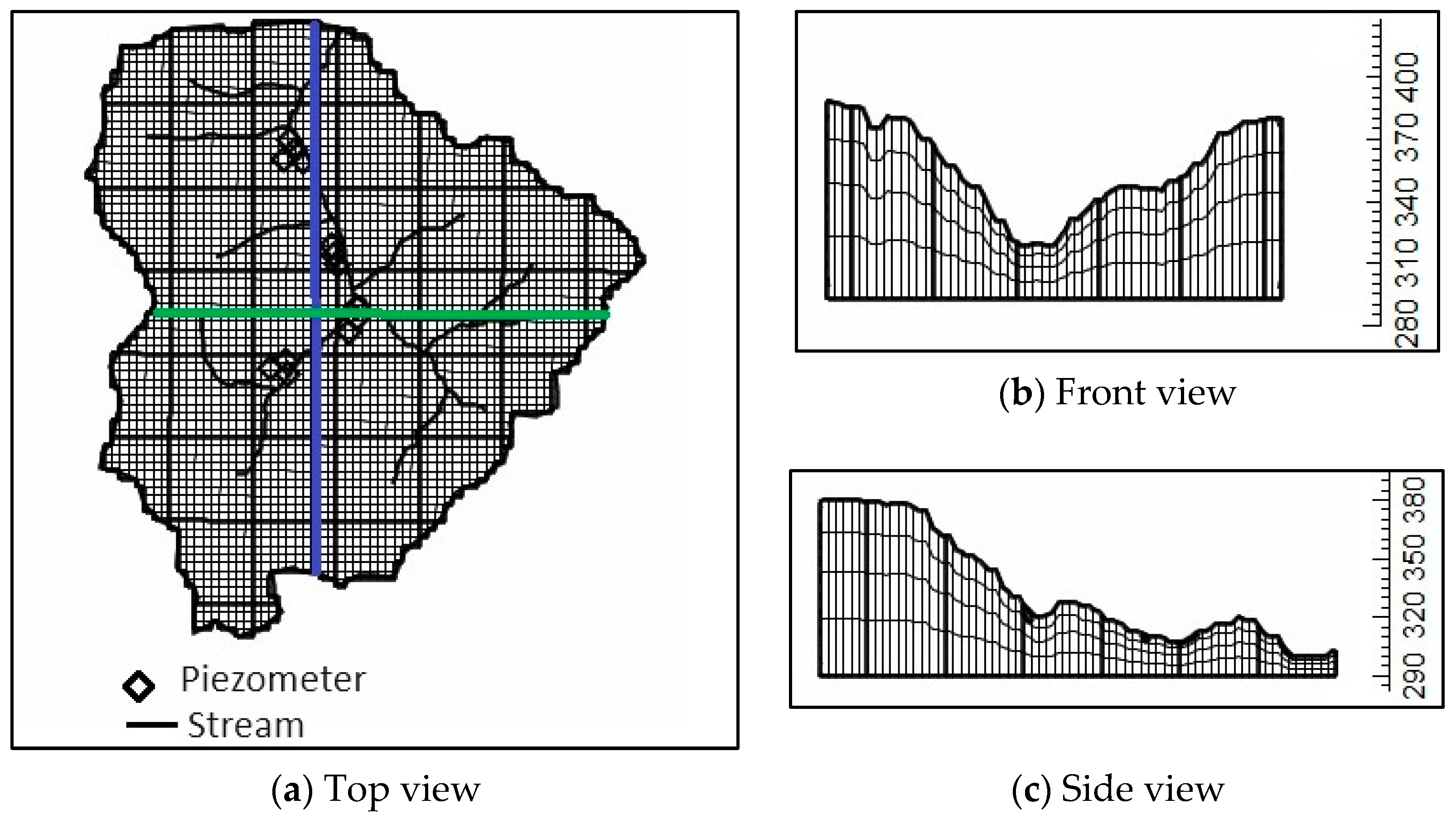
2.2. SGW Flow Model Description and Parameterization

For the current study, an SGW flow model was conceptualized in MODFLOW-2005 [24] for the study reach using ModelMuse (Version 5.1.1.0) [39]. MODFLOW is an international standard for estimating 3D groundwater flow and has been extensively used to understand SW-GW interactions [9,22,25,40]. The 3D flow of GW through porous and permeable media is solved using the following equation [24]:

$$\frac{\partial }{{\partial }_{\mathrm{x}}}\left({\mathrm{K}\mathrm{s}\mathrm{a}\mathrm{t}}_{\mathrm{x}\mathrm{x}}\frac{\partial \mathrm{h}}{\partial \mathrm{x}}\right)+\frac{\partial }{{\partial }_{\mathrm{y}}}\left({\mathrm{K}\mathrm{s}\mathrm{a}\mathrm{t}}_{\mathrm{y}\mathrm{y}}\frac{\partial \mathrm{h}}{\partial \mathrm{y}}\right)+\frac{\partial }{{\partial }_{\mathrm{z}}}\left({\mathrm{K}\mathrm{s}\mathrm{a}\mathrm{t}}_{\mathrm{z}\mathrm{z}}\frac{\partial \mathrm{h}}{\partial \mathrm{z}}\right)-\mathrm{W}={\mathrm{S}}_{\mathrm{s}}\frac{\partial \mathrm{h}}{\partial \mathrm{t}}$$

(1)

where ${\mathrm{K}\mathrm{s}\mathrm{a}\mathrm{t}}_{\mathrm{x}\mathrm{x}},{\mathrm{K}\mathrm{s}\mathrm{a}\mathrm{t}}_{\mathrm{y}\mathrm{y}},$ and ${\mathrm{K}\mathrm{s}\mathrm{a}\mathrm{t}}_{\mathrm{z}\mathrm{z}}$ represent saturated hydraulic conductivities along x, y, and z axes, respectively; h represents the hydraulic head; W represents the volumetric flux per unit volume through the sources and/or sinks of water; S_s represents specific storage of the porous material; and t is time. MODFLOW uses a finite difference approach to solve the GW flow equation (Equation (1)) as, except for simple systems, analytical solutions of Equation (1) are impractical [24]. In the finite difference approach, the aquifer is discretized into 3D grids, and the aquifer properties are considered uniform within each grid cell [24,25].

The study grid comprised 74 rows and 67 columns with uniform cell dimensions of 12 m × 12 m (Figure 2,

Table 1. Model parameter values to simulate shallow groundwater (SGW) flow model using MODFLOW in the study area, West Virginia (WV), USA. The “Range” and “Fitted Value” columns indicate the range of values used in calibration and the best-fit values, respectively. “,” indicates fitted parameter values for vertical SGW layers 1, 2, 3, 4. “—” Indicates values that were not adjusted during calibration.

	Model Parameters	Range	Fitted Value
Grid properties	Rows	—	74
	Columns	—	67
	Layers	—	4
	Cell width along rows	—	12
	Cell width along columns	—	12
Hydrological properties	Hydraulic conductivity (m/d)	0.0038–38	0.38, 0.38, 0.58, 1.28
	Specific Storage	1 × 10−3–9.5 × 10−4	0.013, 0.001, 0.001, 0.001
	Specific yield (m−1)	0.01–0.46	0.02, 0.01, 0.01, 0.01
	Recharge rate (m/d)	5–20% of Precipitation	20% of precipitation
	Stream-bed hydraulic conductivity (m/d)	0.038–50	10
	Stream width (m)	—	2
	Stream-bed thickness (m)	—	1

) and 12,388 active cells. The cell dimension was chosen to provide the needed resolution and computational efficiency [9,25,39,40]. The top elevation was assigned by performing the nearest-neighbor interpolating elevation data collected from the USGS National Elevation Dataset (Figure 1). Given that the study primarily focused on SGW hydrology analysis, the bottom elevation was set at 290 m to ensure stream cells remained above the aquifer bottom. However, to obtain proper resolution for SGW flow, the shallow aquifer was discretized into four vertical layers, the thickness of which increased downwards (Figure 2). The layers were bounded by critical modeling parameters, including saturated hydraulic conductivity (Ksat), specific yield, and specific storage [38]. The hydraulic conductivity of the study area ranged from 0.78 m/d (0.18–0.86 m depth) to 1.98 m/d (1.52 m depth) according to NRCS [37]. However, Abesh and Hubbart [30] estimated Ksat values ranging from a minimum value of 0.62 m/d to a maximum value of 7.29 m/d using the pedotransfer functions [30]. In addition, the soil texture observed by Abesh et al. [25] was sandy, which differed from the NRCS-predicted soil texture of silty loam [37]. Thus, during calibration, a range of Ksat, specific yield, and storage values from the literature [41] were tested for sandy and silty soil textures (Table 1). In addition, previous researchers have empirically estimated GW recharge using precipitation data and suggested that recharge can be around 20–25% for sandy areas and 10–20% for areas more than 40% clay [42]. Thus, 5–20% of precipitation values were tested during calibration as SGW recharge (Table 1). Precipitation data were obtained from a National Oceanic and Atmospheric Administration (NOAA) weather station, approximately five kilometers from the study reach at Morgantown Municipal Airport [43]. The average annual precipitation for 2020–2021 was 1117 mm, with 2021 (1202 mm) experiencing a 16% increase over 2020 (1031 mm). Based on monthly averages, April was the wettest month of 2020 (119 mm), while August was the wettest month of 2021 (183 mm). September (35 mm) and November (29 mm) were the driest months of 2020 and 2021, respectively [31,43].

The creek in the study area was simulated using the “River (RIV)” package of MODFLOW [24]. RIV package is a head-dependent flux boundary, and exchanging flux between the stream and aquifer can be calculated based on the following equation [24].

$${\mathrm{Q}}_{\mathrm{r}\mathrm{i}\mathrm{v}}={\mathrm{C}}_{\mathrm{r}\mathrm{i}\mathrm{v}}({\mathrm{H}}_{\mathrm{r}\mathrm{i}\mathrm{v}}-{\mathrm{H}}_{\mathrm{a}\mathrm{q}\mathrm{u}})$$

(2)

$${\mathrm{C}}_{\mathrm{r}\mathrm{i}\mathrm{v}}=\frac{\mathrm{K}\mathrm{r}\times \mathrm{L}\mathrm{r}\times \mathrm{W}\mathrm{r}}{\mathrm{M}\mathrm{r}}$$

(3)

where ${\mathrm{Q}}_{\mathrm{r}\mathrm{i}\mathrm{v}}$ is the river exchange flux (L/T), ${\mathrm{C}}_{\mathrm{r}\mathrm{i}\mathrm{v}}$ is the streambed conductance (L²/T), ${\mathrm{H}}_{\mathrm{r}\mathrm{i}\mathrm{v}}$ and ${\mathrm{H}}_{\mathrm{a}\mathrm{q}\mathrm{u}}$ are the stream stage and GW head, $\mathrm{K}\mathrm{r},\mathrm{L}\mathrm{r},\mathrm{W}\mathrm{r}$, and Mr are the stream bed conductivity, reach length, width, and streambed thickness. However, the conductance interpretation in ModelMuse was set to “calculated” [39]. Thus, Equation (3) was modified to $(\mathrm{K}\mathrm{r}\times \mathrm{W}\mathrm{r})/\mathrm{M}\mathrm{r}$, the conductance is automatically interpreted for polyline object (stream), and the units are (L/T) [39]. The average observed creek width was 2 m, and depth was a maximum of 0.7 m [32]. The stage value in the RIV package was assigned by interpolation using the monthly stage values from four stream-stage monitoring stations in the study reach. The stream stage was monitored from 2020 to 2021 using Solinst Levelogger pressure transducers (Solinst Canada Ltd., Georgetown, ON, Canada) [44] installed in 5 cm polyvinyl chloride (PVC) stilling wells. A detailed discussion of stream-stage observed values can be found in Abesh et al. [31]. The simulation time of the model was three years, out of which one year of spin-up (2019) and two years (2020–2021) of the period of interest, which was discretized into monthly periods (i.e., stress periods). In addition, the MODFLOW Zonebudget (ZONBUD) (Version 3.01) [45] was used to calculate the SGW and SW interaction separately for downstream (zone 1) and upstream (zone 2) areas (Figure A1).

2.3. SGW Flow Model Calibration and Validation Procedures

The SGW flow model was calibrated in both steady and transient states using observed SGW levels from 13 piezometers of the study reach. The SGW level was monitored using Solinist Levelogger Junior Edge pressure transducers (Solinst Canada Ltd., Georgetown, ON, Canada) [46] placed at the bottom of each piezometer that sensed and stored water depth data. The SGW depth was converted to SGW head (water level elevation above the WGS 1984 datum) by subtracting water depth from land elevation [31]. The average observed SGW values for the study area ranged from 308 m to 330 m between downstream and upstream sites. The standard deviation of SGW levels among co-located piezometers was 1.44 m, 0.67 m, 2.51 m, and 2.26 m, respectively, for sites 1A, 1B, 1C, and 1D. A detailed discussion of the observed SGW level can be found in Abesh et al. [31]. During the steady-state calibration, the simulated SGW head was calibrated using the observed SGW head from 13 piezometers at steady state for January 2020. However, for transient-state calibration, the model was calibrated at a monthly time step for 2020 for 13 piezometers. The hydraulic parameters, including saturated hydraulic conductivity, recharge rate, stream bed conductivity, specific yield, and specific storage, were manually adjusted using a trial-and-error process during calibration [47,48]. The goodness of fit of the observed and simulated SGW head was assessed by the coefficient of determination (R²), root mean square error (RMSE), and mean error (ME). RMSE and ME values near zero indicate better model performance [23,41,48,49]. R² values range from 0 to 1, where close to 1 represents a good fit between observed data and model-simulated output [41,48,49]. After satisfactory goodness of fit was achieved for calibration, the simulated SGW head was validated monthly for 2021. The MODFLOW “Head-Observation package (HOB)” [50] was used to calibrate the model manually.

$$\mathrm{ME}={\sum }_{\mathrm{i}=1}^{\mathrm{n}}\frac{{\mathrm{Y}}_{\mathrm{O}\mathrm{B}\mathrm{S}}-{\mathrm{Y}}_{\mathrm{S}\mathrm{I}\mathrm{M}}}{\mathrm{n}}$$

(4)

$$\mathrm{RMSE}=\sqrt{\frac{\sum _{\mathrm{i}=1}^{\mathrm{N}}{\left[{\mathrm{Y}}_{\mathrm{O}\mathrm{B}\mathrm{S}}-{\mathrm{Y}}_{\mathrm{S}\mathrm{I}\mathrm{M}}\right]}^2}{\mathrm{n}}}$$

(5)

$${\mathrm{R}}^2=\frac{\sum _{\mathrm{i}}{\left[\left({\mathrm{Y}}_{\mathrm{O}\mathrm{B}\mathrm{S}}-{\mathrm{Y}}_{\mathrm{M}\mathrm{E}\mathrm{A}\mathrm{N}}^{\mathrm{O}}\right)\left({\mathrm{Y}}_{\mathrm{S}\mathrm{I}\mathrm{M}}-{\mathrm{Y}}_{\mathrm{M}\mathrm{E}\mathrm{A}\mathrm{N}}^{\mathrm{S}}\right)\right]}^2}{\sum _{\mathrm{i}}{\left({\mathrm{Y}}_{\mathrm{O}\mathrm{B}\mathrm{S}}-{\mathrm{Y}}_{\mathrm{M}\mathrm{E}\mathrm{A}\mathrm{N}}^{\mathrm{O}}\right)}^2\sum {\left({\mathrm{Y}}_{\mathrm{S}\mathrm{I}\mathrm{M}}-{\mathrm{Y}}_{\mathrm{M}\mathrm{E}\mathrm{A}\mathrm{N}}^{\mathrm{S}}\right)}^2}$$

(6)

where ${\mathrm{Y}}_{\mathrm{O}\mathrm{B}\mathrm{S}}$ is the observed data, ${\mathrm{Y}}_{\mathrm{S}\mathrm{I}\mathrm{M}}$ is the simulated data, ${\mathrm{Y}}_{\mathrm{M}\mathrm{E}\mathrm{A}\mathrm{N}}^{\mathrm{S}}$ is mean of simulated data, ${\mathrm{Y}}_{\mathrm{M}\mathrm{E}\mathrm{A}\mathrm{N}}^{\mathrm{O}}$ is the mean of observed data, $\mathrm{i}$ is the $\mathrm{i}$th measured or simulated data, and n is the number of observation data points.

2.4. Nutrient Transport Scenario

After the SGW flow model was calibrated and validated, an experimental contaminant transport scenario was carried out in MT3D-USGS (Version 1.1.0) [51]. MT3D-USGS is an updated version of the solute transport simulator Model Transport Three-Dimensional Model Simulator (MT3DMS) [26,51]. Using the MODFLOW head simulations, MT3D-USGS simulates the nutrient transport using the following equation [51]:

$$\frac{\partial \left(\mathsf{\theta }{\mathrm{C}}^{\mathrm{k}}\right)}{\partial \mathrm{t}}=\frac{\partial }{\partial \mathrm{x}}\left(\mathsf{\theta }{\mathrm{D}}_{\mathrm{i}\mathrm{j}}\frac{\partial {\mathrm{C}}^{\mathrm{k}}}{\partial {\mathrm{x}}_{\mathrm{j}}}\right)-\frac{\partial }{\partial {\mathrm{x}}_{\mathrm{i}}}\left(\mathsf{\theta }{\mathrm{v}}_{\mathrm{i}}{\mathrm{C}}^{\mathrm{k}}\right)+{\mathrm{q}}_{\mathrm{s}}{\mathrm{C}}_{\mathrm{s}}^{\mathrm{k}}+\left(\frac{\partial {\mathrm{C}}^{\mathrm{k}}}{\partial \mathrm{t}}\right)\mathrm{r}\mathrm{x}\mathrm{n}$$

(7)

$$\left(\frac{\partial {\mathrm{C}}^{\mathrm{k}}}{\partial \mathrm{t}}\right)\mathrm{r}\mathrm{x}\mathrm{n}=-\mathrm{K}{\mathrm{C}}^{\mathrm{k}}$$

(8)

where ${\mathrm{C}}^{\mathrm{k}}$ represents the dissolved concentration of species $\mathrm{k}$, $\mathsf{\theta }$ represents the porosity of the subsurface medium, t represents time, x_i,j represents the distance along the respective cartesian coordinate axis, D_ij represents hydrodynamic dispersion coefficient tensor, v_i represents seepage or linear pore water velocity; it is related to the specific discharge or Darcy flux through the relationship. q_s represents the volumetric flow rate per unit volume of aquifer representing fluid sources (positive) and sinks (negative), rxn represents the chemical reaction term, ${\mathrm{C}}_{\mathrm{s}}^{\mathrm{k}}$ represents the concentration of the source or sink flux for species k, and K represents the first-order reaction rate constant.

The soil data analysis showed that the study area’s porosity increased with depth, and the range of porosity was 0.8 to 0.4 [30]. Thus, the model’s porosity was set by layer 1 having a higher porosity (0.8) and layer 4 having a lower porosity (0.4) (

Table 2. List of model parameter values for MT3D_USGS simulation scenario for the study reach, West Virginia (WV), USA. TVD = (third-order total-variation-diminishing method).

	Parameter (Unit)	Values
Advection	Simulation type	Third Order TVD
Dispersion	Longitudinal dispersivity (m)	5
	Horizontal transverse dispersivity ratio	0.5
	Vertical transverse dispersivity ratio	0.05
Porosity	Layer 1, 2, 3, 4	0.8, 0.5, 0.4, 0.4
Chemical reaction	Reaction rate (day−1)	0.07

). For the simulation of advection, third-order Total Variation Diminishing (TVD) was used as this scheme diminishes both numerical dispersion (smearing of concentration fronts) and artificial oscillation (overshoot or undershoot of contaminant transport) [26] (Table 2). NO₃-N has a low sorption capacity. Therefore, the delay factor is set to 1.0 to indicate no sorption following previous studies [52,53,54,55]. The denitrification rate law was specified using first-order kinetic expression [54]. The reaction rate constant was specified as 0.07 day⁻¹. This value is approximately the average rate of denitrification found in soils and aquifers worldwide and represents a half-life of 10 days [12,54,55,56].

Generally, water flow from the aquifer to the stream (gaining stream) was observed in the study area, specifically for the piezometers close to the stream [31]. Thus, to set up an experimental NO₃-N transport scenario, the closest piezometers PA_1A (17 m), PC_1B (18 m), PD_1C (24 m), and PB_1D (8 m) were selected as specific concentration nodes for sites 1A-1D, respectively. The NO₃-N transport scenario was first simulated using advection–dispersion (scenario 1), and the second transport scenario (scenario 2) chemical reaction package was activated to observe the nitrate loss due to denitrification. The specific concentration nodes were forced with the observed nitrate concentration from January 2020 to December 2021, per Abesh et al. [31]. A DR 3900 Laboratory Spectrophotometer [57] and HACH TNTPlus^TM [58] analytes were used to analyze NO₃-N concentrations in monthly SGW grab samples following the standard HACH analytical methods [59]. The observed concentration illustrated an increase in nitrate to 890 µg/L in August 2020 from 110 µg/L in July 2020. From November 2020 to June 2021, a decreasing NO₃-N trend was observed, with high NO₃-N in July 2021 (709 µg/L) [31]. The output concentrations were extracted from the stream cells next to the piezometer from 2020 to 2021 using GW_Chart (Version 4) [60]. The nutrient transport scenario explained NO₃-N loading to stream due to SGW discharge and NO₃-N loss due to denitrification. Thus, this scenario is helpful to strategize future NO₃-N management decisions. In addition, a particle-tracking post-processing MODPATH [61] analysis was performed to analyze the water particle movement and travel time from SGW to stream for the simulation period.

3. Results and Discussion

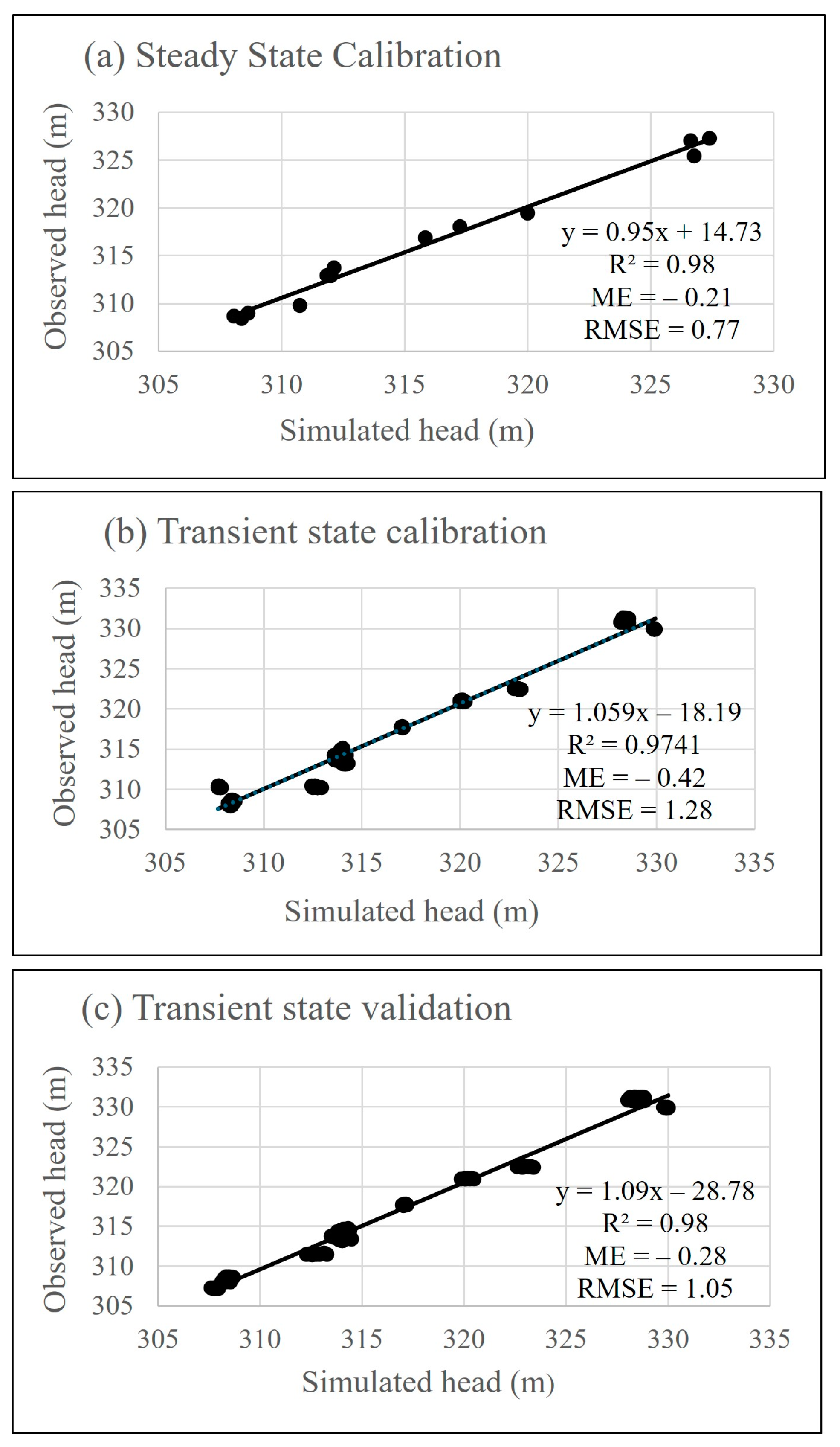
3.1. Calibration and Validation

The SGW MODFLOW simulation was manually calibrated in both steady and transient states. The parameters were fine-tuned during calibration using trial-and-error methods to replicate observations. The best parameter values are represented in Table 1. After a good (as per goodness-of-fit assessments, Section 2.3) agreement between the simulated and observed heads was established, the model was validated for 2021 (Figure 3). Before calibration, the default (uncalibrated) model showed a moderate fit with the observed data, with an RMSE of 10 m. However, the error metric analyses, including reach-scale RMSE and ME after steady- and transient-state calibration, were 0.77 m, −0.21 m, and 1.28 m, −0.41 m, respectively (

Table 3. Error metrics including mean error (ME), root mean square error (RMSE), correlation coefficient (R²), and Nash-Sutcliffe Efficiency (NSE) for steady-state calibration, transient-state calibration, and validation for 13 piezometers in study reach, West Run Watershed, Morgantown, West Virginia (WV).

Model	ME	RMSE	R2
Steady state calibration	−0.21	0.77	0.98
Transient state calibration	−0.42	1.28	0.97
Transient state validation	−0.28	1.05	0.98

). Due to added temporal complexity, the residuals increased from a steady to a transient state. The ME and RMSE values for the validation period were −0.28 and 1.05, respectively (Table 3). The correlation coefficients (R²) for steady- and transient-state-calibrated and -validated models were 0.98, 0.97, and 0.98, indicating good agreement between simulated and observed SGW heads (Table 3). The simulated heads were averaged for piezometer clusters at each monitoring site and compared with the average observed head to analyze the monthly SGW level change per site (Figure 4). All the sites agreed well with the observed data, and the RMSE values ranged from 0.04 m at site 1A to 0.77 at site 1D during calibration (Figure 4). The area’s complex topography contributed to changes in SGW levels, making the calibration process challenging on upstream sites, as corroborated in previous work [23]. However, all the sites responded with greater certainty during validation relative to calibration, with the RMSE ranging from 0.07 for sites 1A and 1D to 0.21 for site 1D (Figure 4).

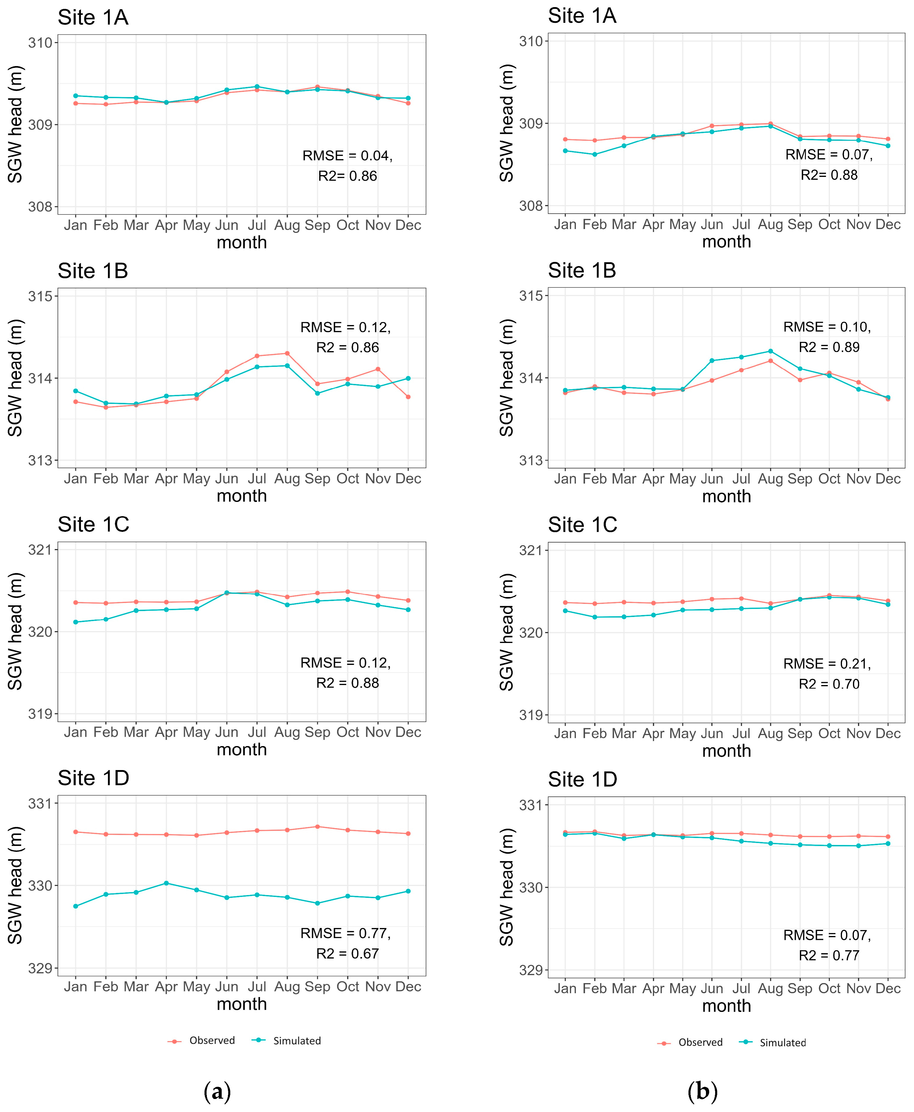
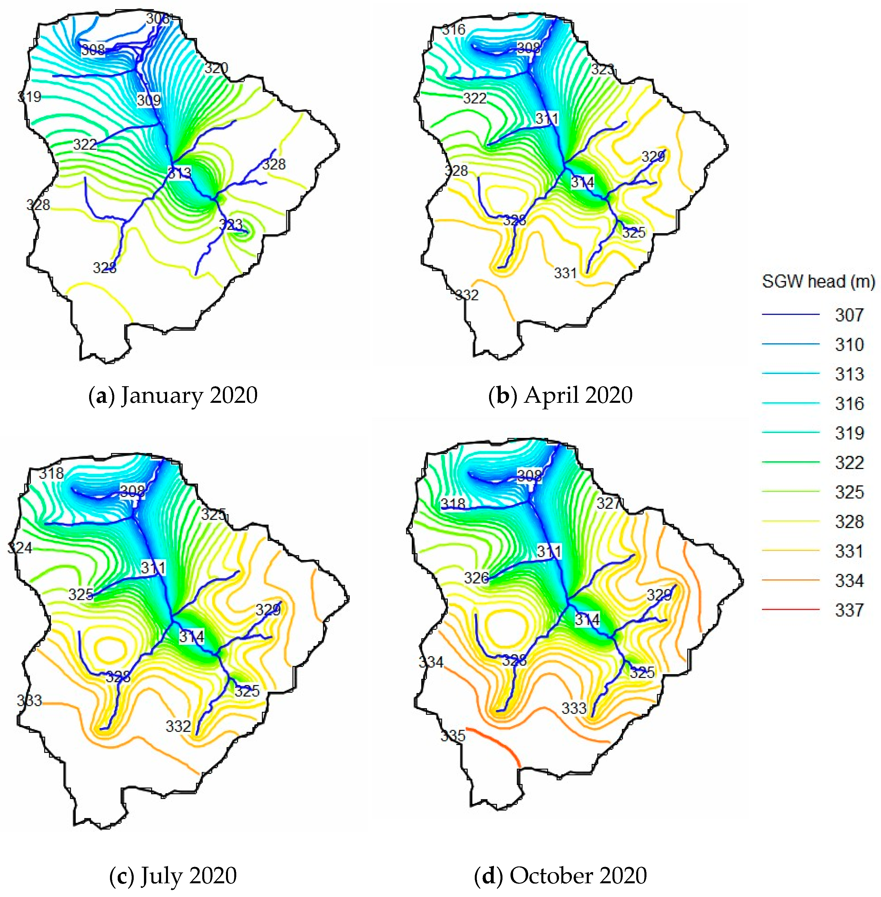
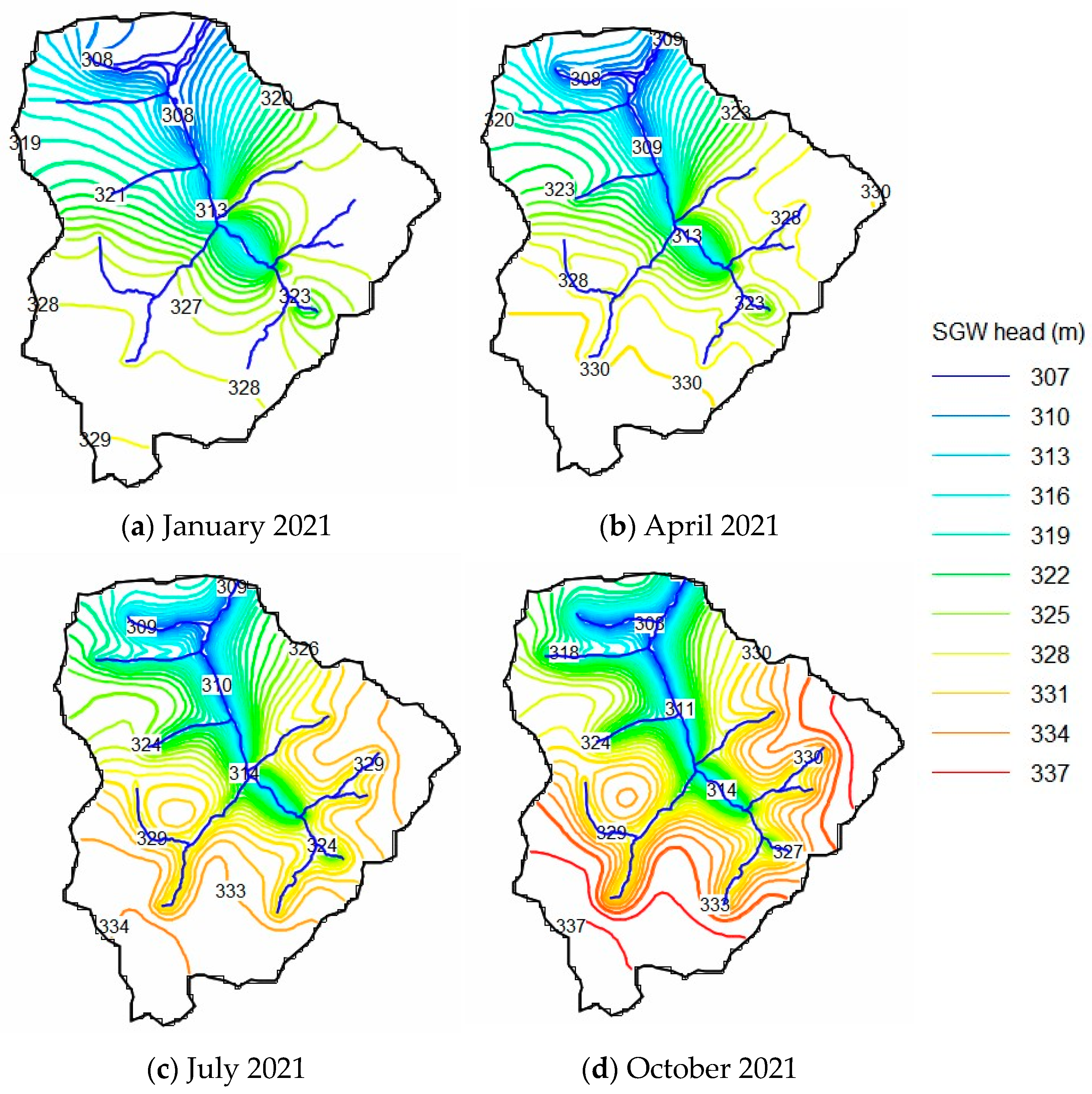
3.2. SGW Simulated Head and Stream-SGW Interaction

The simulated head for the years 2020 and 2021 is represented in Figure 5 and Figure 6. The spatial pattern of head distribution followed the ground surface elevation, with elevated areas exhibiting higher SGW heads and low-elevation areas exhibiting lower SGW heads (Figure 5 and Figure 6). In both years, the lowest groundwater levels were observed near the creek, while higher levels were seen in the northeastern and southern parts of the study area (Figure 5 and Figure 6). In addition, the SGW flow model was forced with a monthly recharge rate due to high precipitation from January to April 2020, ranging from 98 mm in January to 140 mm in April. Consequently, the SGW head was high in January and April 2020, ranging from 332 m to 309 m (Figure 5). Maintaining a similar water level as in July, in October 2020, the water table showed a minor increase, ranging from 335 m to 309 m (Figure 5). With high precipitation from June to August 2021, groundwater heads gradually rose from July to October, reaching a range of 337 m to 308 m in October 2021 (Figure 6). Such results indicated that the SGW head distribution and groundwater flow pattern were relatively stable, with slight monthly fluctuations due to the recharge rates.

From the upstream and downstream zone analysis, a gaining stream condition was observed in the downstream area, with SGW discharge to the creek averaging 16% higher in 2020 and 18% higher in 2021 compared to the creek seepage. The downstream area exhibited SGW discharge ranging from 948 m³/day to 907 m³/day and creek seepage ranging from 802 m³/day to 790 m³/day in 2020 (Figure 7). Additionally, in 2021, SGW input to the creek in the downstream area ranged from 891 m³/day to 978 m³/day, while creek seepage ranged from 796 m³/day to 800 m³/day (Figure 7). However, a monthly gaining–losing stream condition was observed in the upstream area. For example, stream seepage to the aquifer was higher in January, June, and September 2020, and a losing stream condition was observed. For all the other months in 2020, a gaining stream condition prevailed. In 2021, January to April and May to December exhibited losing and gaining stream conditions, respectively. The monthly fluctuations between gaining and losing stream conditions in the upstream reach were influenced by precipitation events and recharge rates. Generally, the capillary fringe zone (where GW is held under tension) above the water table is disrupted during high-precipitation events, and GW rises on top of the fringe [6,7,62]. Thus, the rapid increase in GW head near the stream can contribute substantially to the stream [6,7,62]. In addition, if the water table depth is shallow (SGW), a minimal amount of percolated water could trigger the gaining stream condition [6,7,62]. This continuous water transfer between the aquifer and stream indicates a well-connected SW and SGW system [6,7,9,62,63]. Similarly, Sisay et al. [63] concluded that MODFLOW successfully simulated lateral fluxes between the river and GW, demonstrating a connected gaining and losing system due to a shallow water table. The authors reported groundwater discharge to the streams of 4940 m³/day, while stream seepage was lower, up to 675 m³/day. During their study, Chinnasamy and Hubbart [9] also observed alternating gaining and losing stream conditions. They suggested that stream water lost to the aquifer (losing stream) may reemerge in the stream during high-recharge periods (precipitation events) depending on flow path and residence time. The interconnected SW-SGW system in the study area allows highly dissolved nutrients from SGW to be transported to SW, as corroborated by [18,19]. For example, Kwon et al. [18] identified gaining stream conditions in the upland, high-elevation areas, suggesting that elevated SW nitrogen (N) and phosphorus (P) concentrations were associated with SGW flow into the stream during gaining stream conditions. Therefore, quantifying SGW and SW exchange can assist water resource management and environmental conservation efforts by delineating nutrient transport pathways and analyzing nutrient dilution and attenuation capacities [6,7,18].

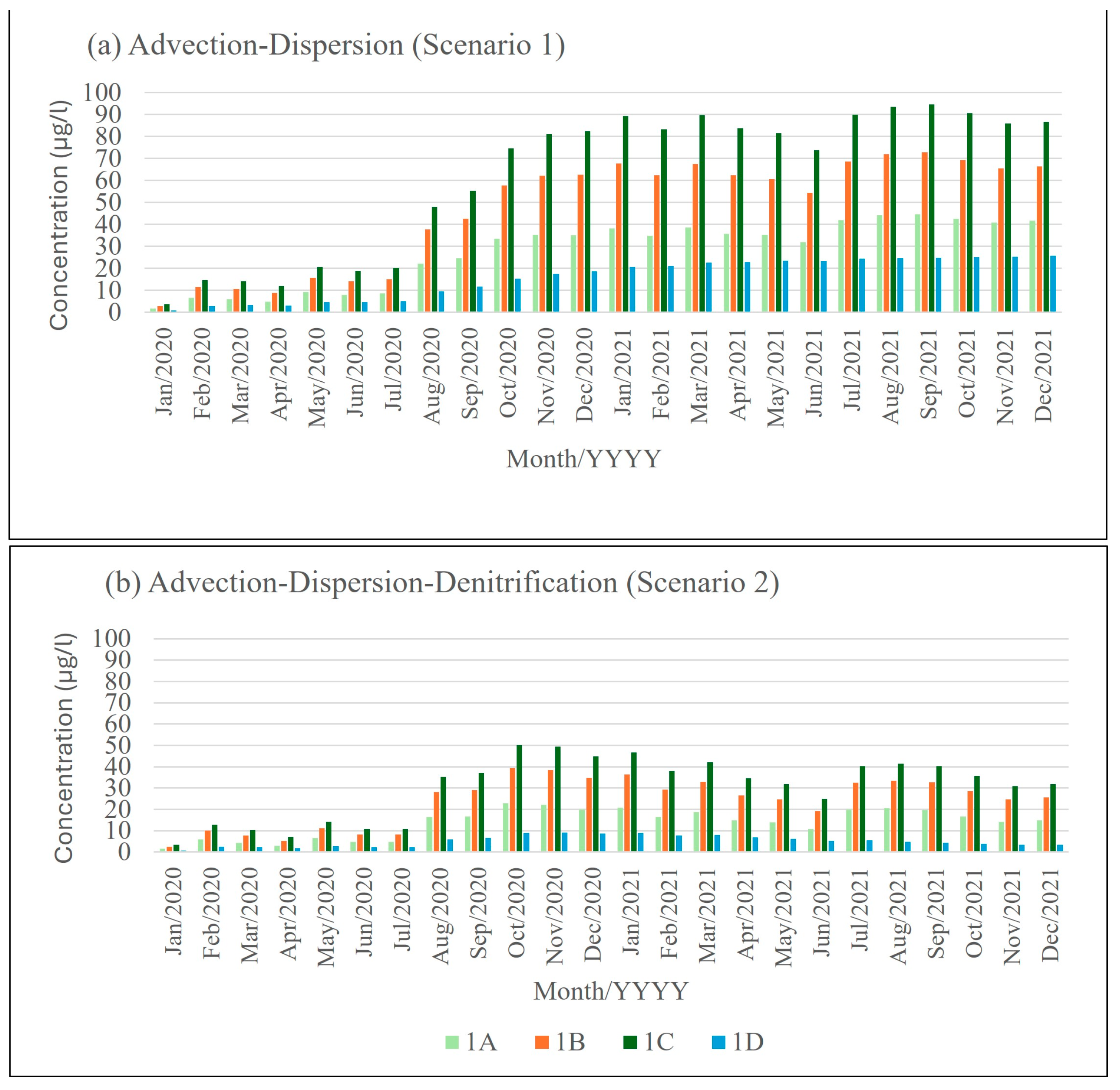
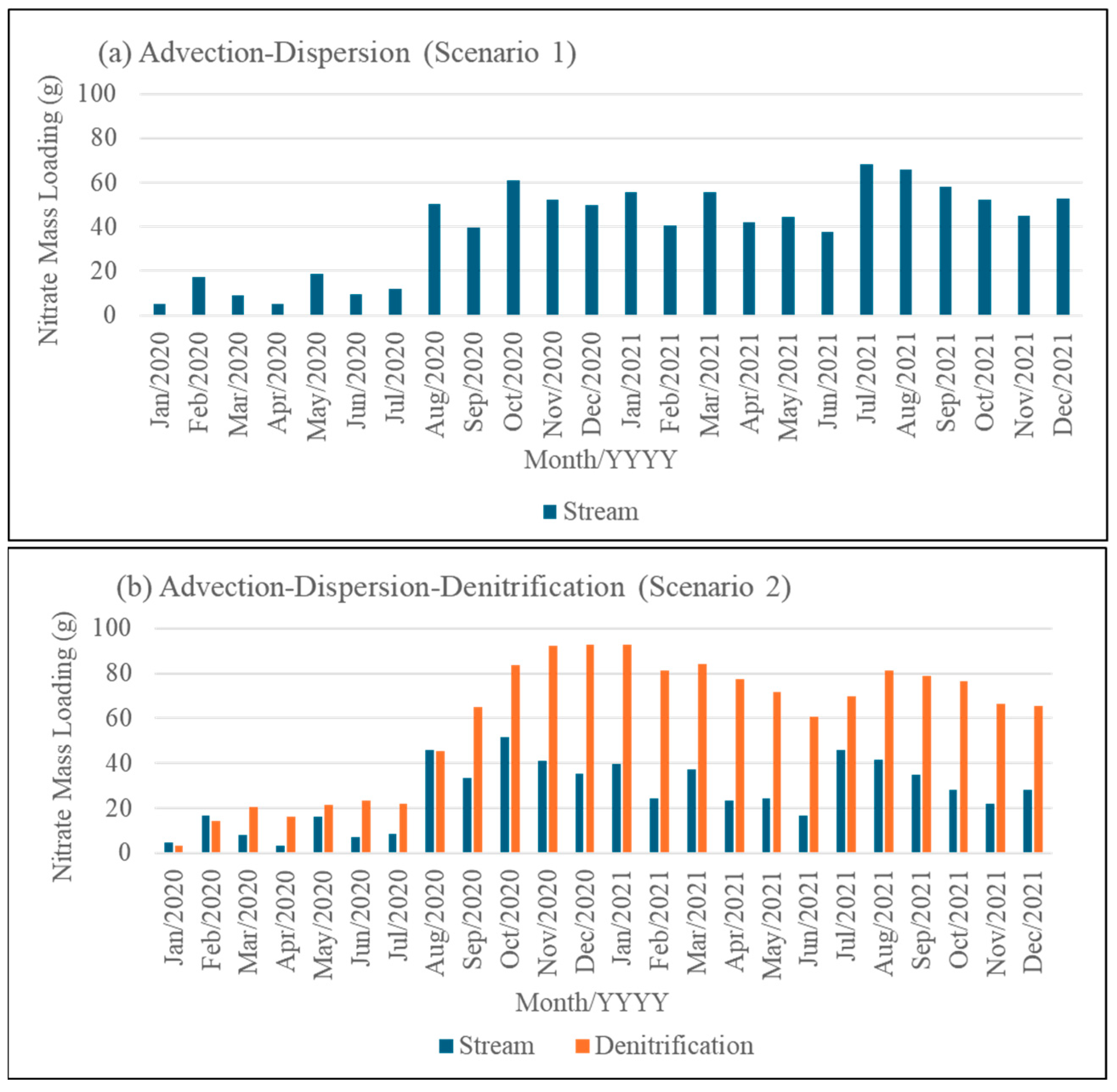
3.3. Nutrient Transport

The MT3D simulation revealed lateral transport of NO₃-N from the shallow aquifer to stream cells in the model, with the highest nitrate concentrations observed in stream cells in 1C, followed by 1B, 1A, and 1D (Figure 8). The variation in NO₃-N transport between sites is attributed to differences in SGW flow velocities, as MT3D utilizes velocity values from MODFLOW SGW simulation to solve nutrient transport routines [26,51]. In Scenario 1, representing advection–dispersion, stream NO₃-N concentrations remained low from January 2020 to July 2020, ranging from 0.8 µg/L for 1D in January to 20 µg/L for 1C in July (Figure 8a). Concentrations increased from August 2020 for all sites, with notably high values observed during the fall months (August to November) in both years (Figure 8a). In Scenario 2, accounting for chemical reactions, similar transport trends were observed with elevated NO₃-N in the fall months (October and November) (Figure 8b). However, NO₃-N transport to the stream was lower than Scenario 1 due to NO₃-N loss to denitrification, resulting in peak concentrations of 50 µg/L in October 2020 and 41 µg/L in August 2021 (Figure 8b). Sun et al. [64] similarly identified decreased NO₃-N transport in SW due to SGW denitrification while studying a riparian floodplain area, and the reduction of NO₃-N was in a range of 5 mg/L to 10 mg/L.

From Scenario 1, a cumulative nitrate loss of 947 g was observed from the shallow aquifer to the stream between 2020 and 2021. In the upstream areas (zone 2), 464 g of nitrate was transferred from the SGW to the stream, while in the downstream sites (zone 1), the cumulative transfer was 483 g. The monthly average nitrate loss from the aquifer to the stream was 39 g for 2020–2021, with the average monthly nitrate loss in 2021 (51 g) higher than in 2020 (27 g). For 2020, elevated NO₃-N loading to the stream occurred in August, October, and November (60 g), while in 2021, July showed high NO₃-N loading of 69 g (Figure 9a). Considering chemical reactions (Scenario 2), a total of 639 g of nitrate was lost from the SGW to the stream from 2020 to 2021; however, 1406 g of nitrate was lost due to denitrification (Figure 9b). These findings align with previous research [52,53,54], where denitrification was identified as the primary nitrogen sink. In January and February 2020, NO₃-N loss from SGW to the stream initially exceeded denitrification (Figure 9b). However, starting in March 2020, denitrification surpassed the NO₃-N loss to stream, except for August 2020 (Figure 9b). The NO₃-N loss by denitrification was highest during the fall of 2020 (October–December) and late summer and fall of 2021 (August–October) (Figure 9b). Moreover, particle tracking using MODPATH revealed a long travel time (70 to 1095 days) for particles released from SGW piezometers to the stream (

Table 4. MODPATH particle travel time (days) from piezometers to stream cells for the study reach West Virginia (WV), USA, for the simulation period (spin up (2019) + 2020–2021). Notes: The values in parentheses represent the piezometer distance from the creek. “>” = more than.

Site	Piezometer	Travel Time (Days)
1A	PA_1A (19 m)	820
	PB_1A (21 m)	680
	PC_1A (55 m)	>1095
	PD_1A (16 m)	80
1B	PA_1B (28 m)	780
	PB_1B (27 m)	770
	PC_1B (18 m)	730
1C	PA_1C (40 m)	1080
	PB_1C (80 m)	>1095
	PD_1C (24 m)	840
1D	PA_1D (43 m)	>1095
	PC_1D (31 m)	>1095
	PB_1D (8 m)	70

), indicating a low velocity and long residence time for SGW nutrients. This prolonged residence time would allow SGW nutrients to transform, such as denitrification [9,13,53], further supporting the high NO₃-N loss by denitrification. In addition, Wang et al. [54] observed from lab analysis and MT3D modeling that denitrification played a significant role in NO₃-N attenuation, primarily due to low water velocity and high NO₃-N residence time. The authors noted that under high velocity, the denitrification rate decreased by approximately 30% due to the reduced contact of NO₃-N with sediments. Overall, particles released from piezometers near the stream reached nearby cells within three years (including spin-up and simulation time) (Table 4). Conversely, particles from piezometers farther from the stream did not reach the stream cells within the same timeframe, so they remained in the aquifer (Table 4). At downstream site 1B, particles from all piezometers reached stream cells with travel times of 730, 770, and 780 days to cover distances of 18 m, 27 m, and 28 m, respectively. Conversely, at upstream site 1C, particles traveled 24 m in 840 days, while 40 m was covered in 1080 days (Table 4).

3.4. Limitations and Implications

The simulated SGW flow model in MODFLOW provided essential insights into SGW flow dynamics and the interaction between SGW and the stream water in riparian wetlands of a mixed land use catchment in West Virginia. Notably, the current study offers an opportunity to understand the NO₃-N transport and loading from SGW to the stream and NO₃-N loss due to denitrification. This SGW simulation and NO₃-N scenario analysis will affect water and land management strategies by identifying SW-SGW interconnections, volumetric transfer between stream and SGW, and nutrient transport pathways. However, the current study has several limitations that are important to acknowledge in order to motivate future studies. For example, evapotranspiration (ET) is an important water balance component, specifically when analyzing SGW, which is close to the land surface [1]. However, there exists no record of ET during the study period (2020–2021) for the study area; therefore, ET was not used in the current model. The estimated recharge rate during model construction was predicted to be low to compensate for the absence of ET. In addition, the absence of bore log data to indicate subsurface geological information and textural change could also introduce simulation uncertainties. Despite these limitations, the uncertainties were addressed by calibrating and validating simulated and observed SGW levels with good agreement. In addition, the NO₃-N transport scenario was experimental and limited due to the absence of proper input properties and observed analysis of source and sink subsurface characteristics. For example, the reaction rate is an essential input parameter to estimate NO₃-N loss by denitrification, estimated from previous studies and not validated.

Given that denitrification is a complex biochemical reaction influenced by various factors, such as the presence of microbial population and organic carbon, redox potential, and sediment texture, additional lab experiments, including soil column experiments or isotope analysis, are needed to validate denitrification rates [13,54,65]. Moreover, stable isotopes may offer more reliable insights into the source and sink behavior of SGW NO₃-N [66], validating the MT3D transport of SGW NO₃-N to SW. Currently, integrated models, such as the Soil Water Assessment Tool (SWAT)-MODFLOW [12] and SWAT-LUD [64] models, hold promise for quantifying denitrification in the soil profile and SGW, allowing for the estimation of water exchange and nitrate attenuation in wetland areas on a catchment scale. Therefore, future research endeavors should prioritize employing fully integrated models to quantify the rate of soil nutrient mobilization, denitrification, and delivery to surface water.

4. Conclusions

A study on shallow groundwater (SGW) flow dynamics and the hydrologic interaction between SGW and stream water (SW) was conducted using MODFLOW in the riparian wetland of a mixed land use catchment in the Appalachian region of West Virginia, USA. SGW levels from 13 piezometers were calibrated and validated by the SGW head under steady and transient states. The calibration and validation error metrics (steady state: R² = 0.98, ME = −0.21, RMSE = 0.77; transient state: R² = 0.97, ME = −0.41, RMSE = 1.28; validation: R² = 0.97, ME = −0.28, RMSE = 1.05) indicated good agreement between observed and simulated SGW head. The SGW head distribution was relatively stable, with slight monthly fluctuations due to recharge rate variations. A losing stream condition was observed downstream, with SGW discharge ranging from 948 to 907 m³/day and creek seepage from 802 to 790 m³/day in 2020, and SGW input to the stream ranging from 891 to 978 m³/day and creek seepage from 796 to 800 m³/day in 2021. Upstream areas showed a monthly alternating gaining–losing stream condition. An experimental MT3D transport scenario revealed the lateral transport of NO₃-N from the aquifer to stream cells, with the highest concentrations in stream cells 1C, followed by 1B, 1A, and 1D. The advection–dispersion scenario simulated a cumulative nitrate loss of 947 g from the SGW to the stream between 2020 and 2021, while denitrification accounted for 1406 g of NO₃-N loss, indicating its importance as a nitrogen sink. Particle tracking with MODPATH suggested a longer residence time for SGW nutrients, supporting efficient nitrogen transformation through denitrification. This research, a pioneering effort in numerically modeling hydrologic and nutrient interactions in riparian wetlands within the Appalachian area, provides baseline modeling predictions to enhance future SW-SGW-integrated models and water management strategies.

References

1. Hare, D.K.; Helton, A.M.; Johnson, Z.C.; Lane, J.W.; Briggs, M.A. Continental-Scale Analysis of Shallow and Deep Groundwater Contributions to Streams. Nat. Commun. 2021, 12, 1450. [Google Scholar] [CrossRef] [PubMed]
2. Chen, S.; Wu, W.; Hu, K.; Li, W. The Effects of Land Use Change and Irrigation Water Resource on Nitrate Contamination in Shallow Groundwater at County Scale. Ecol. Complex. 2010, 7, 131–138. [Google Scholar] [CrossRef]
3. Taylor, C.A.; Stefan, H.G. Shallow Groundwater Temperature Response to Climate Change and Urbanization. J. Hydrol. 2009, 375, 601–612. [Google Scholar] [CrossRef]
4. Barron, O.V.; Barr, A.D.; Donn, M.J. Effect of Urbanisation on the Water Balance of a Catchment with Shallow Groundwater. J. Hydrol. 2013, 485, 162–176. [Google Scholar] [CrossRef]
5. Robinson, C. Review on Groundwater as a Source of Nutrients to the Great Lakes and Their Tributaries. J. Great Lakes Res. 2015, 41, 1. [Google Scholar] [CrossRef]
6. Sophocleous, M. Interactions between Groundwater and Surface Water: The State of the Science. Hydrogeol. J. 2002, 10, 52–67. [Google Scholar] [CrossRef]
7. Banerjee, D.; Ganguly, S. A Review on the Research Advances in Groundwater–Surface Water Interaction with an Overview of the Phenomenon. Water 2023, 15, 1552. [Google Scholar] [CrossRef]
8. Fleckenstein, J.H.; Krause, S.; Hannah, D.M.; Boano, F. Groundwater-Surface Water Interactions: New Methods and Models to Improve Understanding of Processes and Dynamics. Adv. Water Resour. 2010, 33, 1291–1295. [Google Scholar] [CrossRef]
9. Chinnasamy, P.; Hubbart, J.A. Potential of MODFLOW to Model Hydrological Interactions in a Semikarst Floodplain of the Ozark Border Forest in the Central United States. Earth Interact. 2014, 18, 1–24. [Google Scholar] [CrossRef]
10. Kurylyk, B.L.; MacQuarrie, K.T.B.; Caissie, D.; McKenzie, J.M. Shallow Groundwater Thermal Sensitivity to Climate Change and Land Cover Disturbances: Derivation of Analytical Expressions and Implications for Stream Temperature Modeling. Hydrol. Earth Syst. Sci. 2015, 19, 2469–2489. [Google Scholar] [CrossRef]
11. Donner, S.D.; Kucharik, C.J.; Foley, J.A. Impact of Changing Land Use Practices on Nitrate Export by the Mississippi River. Glob. Biogeochem. Cycles 2004, 18. [Google Scholar] [CrossRef]
12. Wei, X.; Bailey, R.T.; Records, R.M.; Wible, T.C.; Arabi, M. Comprehensive Simulation of Nitrate Transport in Coupled Surface-Subsurface Hydrologic Systems Using the Linked SWAT-MODFLOW-RT3D Model. Environ. Model. Softw. 2019, 122, 104242. [Google Scholar] [CrossRef]
13. White, J.R.; Reddy, K.R. Biogeochemical Dynamics I: Nitrogen Cycling in Wetlands. In The Wetlands Handbook; Maltby, E., Barker, T., Eds.; Wiley: Hoboken, NJ, USA, 2009; pp. 213–227. ISBN 978-0-632-05255-4. [Google Scholar]
14. Hefting, M.M.; Clement, J.-C.; Bienkowski, P.; Dowrick, D.; Guenat, C.; Butturini, A.; Topa, S.; Pinay, G.; Verhoeven, J.T.A. The Role of Vegetation and Litter in the Nitrogen Dynamics of Riparian Buffer Zones in Europe. Ecol. Eng. 2005, 24, 465–482. [Google Scholar] [CrossRef]
15. Chinnasamy, P.; Hubbart, J.A. Stream and Shallow Groundwater Nutrient Concentrations in an Ozark Forested Riparian Zone of the Central USA. Environ. Earth Sci. 2015, 73, 6577–6590. [Google Scholar] [CrossRef]
16. Reay, W.G.; Gallagher, D.L.; Simmons, G.M. Groundwater discharge and its impact ON surface water quality IN a chesapeake bay inlet 1. J. Am. Water Resour. Assoc. 1992, 28, 1121–1134. [Google Scholar] [CrossRef]
17. Ouyang, Y. Estimation of Shallow Groundwater Discharge and Nutrient Load into a River. Ecol. Eng. 2012, 38, 101–104. [Google Scholar] [CrossRef]
18. Kwon, H.-I.; Koh, D.-C.; Cho, B.-W.; Jung, Y.-Y. Nutrient Dynamics in Stream Water and Groundwater in Riparian Zones of a Mesoscale Agricultural Catchment with Intense Seasonal Pumping. Agric. Water Manag. 2022, 261, 107336. [Google Scholar] [CrossRef]
19. Ruiz, L.; Abiven, S.; Martin, C.; Durand, P.; Beaujouan, V.; Molénat, J. Effect on Nitrate Concentration in Stream Water of Agricultural Practices in Small Catchments in Brittany: II. Temporal Variations and Mixing Processes. Hydrol. Earth Syst. Sci. 2002, 6, 507–514. [Google Scholar] [CrossRef]
20. Schmalz, B.; Springer, P.; Fohrer, N. Variability of Water Quality in a Riparian Wetland with Interacting Shallow Groundwater and Surface Water. Z. Pflanzenernähr. Bodenk. 2009, 172, 757–768. [Google Scholar] [CrossRef]
21. Karlović, I.; Posavec, K.; Larva, O.; Marković, T. Numerical Groundwater Flow and Nitrate Transport Assessment in Alluvial Aquifer of Varaždin Region, NW Croatia. J. Hydrol. Reg. Stud. 2022, 41, 101084. [Google Scholar] [CrossRef]
22. Rajaeian, S.; Ketabchi, H.; Ebadi, T. Investigation on Quantitative and Qualitative Changes of Groundwater Resources Using MODFLOW and MT3DMS: A Case Study of Hashtgerd Aquifer, Iran. Environ. Dev. Sustain. 2023, 26, 4679–4704. [Google Scholar] [CrossRef]
23. Colombo, L.; Alberti, L.; Mazzon, P.; Formentin, G. Transient Flow and Transport Modelling of an Historical CHC Source in North-West Milano. Water 2019, 11, 1745. [Google Scholar] [CrossRef]
24. Harbaugh, A.W. MODFLOW-2005: The U.S. Geological Survey Modular Ground-Water Model—The Ground-Water Flow Process. 2005. Available online: https://pubs.usgs.gov/publication/tm6A16 (accessed on 1 January 2024).
25. Brunner, P.; Simmons, C.T.; Cook, P.G.; Therrien, R. Modeling Surface Water-Groundwater Interaction with MODFLOW: Some Considerations. Ground Water 2010, 48, 174–180. [Google Scholar] [CrossRef] [PubMed]
26. Zheng, C.; Wang, P.P. MT3DMS: A Modular Three-Dimensional Multispecies Transport Model for Simulation of Advection, Dispersion, and Chemical Reactions of Contaminants in Groundwater Systems; Strategic Environmental Research and Development Program; Documentation and User’s Guide; U.S. Army Corps of Engineers: Washington, DC, USA, 1999; pp. 1–40.
27. Jazi, R.S.; Eckstein, Y. Simulation of Groundwater Flow System in Alluvium and Fractured Weathered Bedrock Zone: Sand Lick Watershed, Boone County, West Virginia, USA. Environ. Earth Sci. 2015, 74, 2247–2258. [Google Scholar] [CrossRef]
28. U.S. Geological Survey, Washington Water Science Center; Kozar, M.D.; McCoy, K.J. Use of modflow drain package for simulating inter-basin transfer of groundwater in abandoned coal mines. JASMR 2012, 1, 27–43. [Google Scholar] [CrossRef]
29. Boettner, F.; Clingerman, J.; McIlmoil, R.; Hansen, E.; Hartz, L.; Hereford, A.; Vanderberg, M.; Arano, K.; Deng, J.; Strager, J.; et al. An Assessment of Natural Assets in the Appalachian Region: Water Resources; Appalachian Regional Commission: Washington, DC, USA, 2014; 76p.
30. Abesh, B.F.; Hubbart, J.A. A Comparison of Saturated Hydraulic Conductivity (Ksat) Estimations from Pedotransfer Functions (PTFs) and Field Observations in Riparian Seasonal Wetlands. Water 2023, 15, 2711. [Google Scholar] [CrossRef]
31. Abesh, B.F.; Anderson, J.T.; Hubbart, J.A. Surface Water (SW) and Shallow Groundwater (SGW) Nutrient Concentrations in Riparian Wetlands of a Mixed Land-Use Catchment. Land 2024, 13, 409. [Google Scholar] [CrossRef]
32. Heck, Z.A. Development of Multi-Catchment Rating Curves for Streams of Appalachian Mixed-Land-Use Watersheds: Preliminary Results; West Virginia University Libraries: Morgantown, WV, USA, 2021. [Google Scholar]
33. Gootman, K.S.; Hubbart, J.A. Characterization of Sub-Catchment Stream and Shallow Groundwater Nutrients and Suspended Sediment in a Mixed Land Use, Agro-Forested Watershed. Water 2023, 15, 233. [Google Scholar] [CrossRef]
34. Hubbart, J.A.; Kellner, E.; Zeiger, S.J. A Case-Study Application of the Experimental Watershed Study Design to Advance Adaptive Management of Contemporary Watersheds. Water 2019, 11, 2355. [Google Scholar] [CrossRef]
35. Kellner, E.; Hubbart, J.; Stephan, K.; Morrissey, E.; Freedman, Z.; Kutta, E.; Kelly, C. Characterization of Sub-Watershed-Scale Stream Chemistry Regimes in an Appalachian Mixed-Land-Use Watershed. Environ. Monit. Assess. 2018, 190, 586. [Google Scholar] [CrossRef]
36. Wright, E.L.; Charles, H.D.; Sponaugle, K.; Cole, C.; Ammons, J.T.; Gorman, J.; Childs, F.D.; Soil Conservation Service. Soil Survey of Marion and Monongalia Counties, West Virginia. 1982. Available online: https://www.govinfo.gov/content/pkg/GOVPUB-A57-PURL-LPS105834/pdf/GOVPUB-A57-PURL-LPS105834.pdf (accessed on 15 March 2022).
37. Soil Survey Staff, Natural Resources Conservation Service, United States Department of Agriculture. Soil Survey Geographic Database (SSURGO). Available online: https://www.nrcs.usda.gov/resources/data-and-reports/soil-survey-geographic-database-ssurgo (accessed on 28 January 2023).
38. Kozar, B.M.D.; Mathes, M.V. Aquifer-Characteristics Data for West Virginia; Water Investigations Report 01-4036; U.S. Geological Survey: Reston, VA, USA, 2001.
39. Winston, R.B. ModelMuse: A Graphical User Interface for MODFLOW-2005 and PHAST; Techniques and Methods 6—A29; U.S. Geological Survey: Reston, VA, USA, 2009; 52p.
40. Abesh, B.; Liu, G.; Vázquez-Ortega, A.; Gomezdelcampo, E.; Roberts, S. Cyanotoxin Transport from Surface Water to Groundwater: Simulation Scenarios for Lake Erie. J. Great Lakes Res. 2022, 48, 695–706. [Google Scholar] [CrossRef]
41. Anderson, M.P.; Woessner, W.W.; Hunt, R.J. Applied Groundwater Modeling: Simulation of Flow and Advective Transport; Academic Press: Cambridge, MA, USA, 2015. [Google Scholar]
42. Andualem, T.G.; Demeke, G.G.; Ahmed, I.; Dar, M.A.; Yibeltal, M. Groundwater Recharge Estimation Using Empirical Methods from Rainfall and Streamflow Records. J. Hydrol. Reg. Stud. 2021, 37, 100917. [Google Scholar] [CrossRef]
43. NOAA National Centers for Environmental Information. Local Climatological Data (LCD). 2010. Available online: https://www.ncei.noaa.gov/products/land-based-station/local-climatological-data (accessed on 1 January 2024).
44. Solinst. Solnist Levelogger Pressure Transducer. 2020. Available online: https://www.solinst.com/products/products-dataloggers.php (accessed on 8 August 2021).
45. Harbaugh, A.W. A Computer Program for Calculating Subregional Water Budgets Using Results from the U.S. Geological Survey Modular Three-Dimensional Finite-Difference Ground-Water Flow Model; Open-File Report 90-392; U.S. Geological Survey: Reston, VA, USA, 1990.
46. Solinst. Solinist Levelogger Junior Edge Pressure Transducers. 2020. Available online: https://www.solinst.com/onthelevel-news/water-level-monitoring/water-level-datalogging/levelogger-data-critical-for-water-and-leachate-management-at-a-queensland-landfill/ (accessed on 8 August 2021).
47. Behera, A.K.; Pradhan, R.M.; Kumar, S.; Chakrapani, G.J.; Kumar, P. Assessment of Groundwater Flow Dynamics Using MODFLOW in Shallow Aquifer System of Mahanadi Delta (East Coast), India. Water 2022, 14, 611. [Google Scholar] [CrossRef]
48. Shakeri, R.; Nassery, H.R.; Ebadi, T. Numerical Modeling of Groundwater Flow and Nitrate Transport Using MODFLOW and MT3DMS in the Karaj Alluvial Aquifer, Iran. Environ. Monit. Assess. 2023, 195, 242. [Google Scholar] [CrossRef]
49. Moriasi, D.N.; Wilson, B.N.; Douglas-Mankin, K.R.; Arnold, J.G.; Gowda, P.H. Hydrologic and Water Quality Models: Use, Calibration, and Validation. Lebensversicherungsmedizin 2012, 55, 1241–1247. [Google Scholar]
50. Hill, M.C.; Banta, E.R.; Harbaugh, A.W.; Anderman, E.R. MODFLOW-2000, the U.S. Geological Survey Modular Ground-Water Model; User Guide to the Observation, Sensitivity, and Parameter-Estimation Processes and Three Post-Processing Programs; Open-File Report 2000-184; U.S. Geological Survey: Reston, VA, USA, 2000; 209p.
51. Bedekar, V.; Morway, E.D.; Langevin, C.D.; Tonkin, M.J. MT3D-USGS Version 1: A U.S. Geological Survey Release of MT3DMS Updated with New and Expanded Transport Capabilities for Use with MODFLOW; Techniques and Methods 6—A53; U.S. Geological Survey: Reston, VA, USA, 2016.
52. Wang, Y.; Shao, M.; Liu, Z.; Horton, R. Regional-Scale Variation and Distribution Patterns of Soil Saturated Hydraulic Conductivities in Surface and Subsurface Layers in the Loessial Soils of China. J. Hydrol. 2013, 487, 13–23. [Google Scholar] [CrossRef]
53. Zhang, L.; Li, X.; Han, J.; Lin, J.; Dai, Y.; Liu, P. Identification of Surface Water—Groundwater Nitrate Governing Factors in Jianghuai Hilly Area Based on Coupled SWAT-MODFLOW-RT3D Modeling Approach. Sci. Total Environ. 2024, 912, 168830. [Google Scholar] [CrossRef]
54. Wang, S.; Wu, B.; Wang, Y.; Wang, X. Nitrate Migration and Transformation in Low Permeability Sediments: Laboratory Experiments and Modeling. Water 2023, 15, 2528. [Google Scholar] [CrossRef]
55. Conan, C.; Bouraoui, F.; Turpin, N.; de Marsily, G.; Bidoglio, G. Modeling Flow and Nitrate Fate at Catchment Scale in Brittany (France). J. Environ. Qual. 2003, 32, 2026–2032. [Google Scholar] [CrossRef]
56. Bailey, R.T.; Baù, D.A.; Gates, T.K. Estimating Spatially-Variable Rate Constants of Denitrification in Irrigated Agricultural Groundwater Systems Using an Ensemble Smoother. J. Hydrol. 2012, 468, 188–202. [Google Scholar] [CrossRef]
57. HACH. DR3900 Laboratory Spectrophotometer for Water Analysis|Hach USA. 2020. Available online: https://au.hach.com/spectrophotometers/dr3900-laboratory-spectrophotometer-for-water-analysis/family?productCategoryId=22218653565 (accessed on 8 August 2021).
58. HACH. TNTplus Vial Chemistries. 2020. Available online: https://www.hach.com/products/chemistries/tntplus (accessed on 8 August 2021).
59. HACH. Hach Company TNTplus 835/836 Nitrate Method 10206 Spectrophotometric Measurement of Nitrate in Water and Wastewater. 2013. Available online: https://cdn.bfldr.com/7FYZVWYB/at/wv5rq9452s3bkwxh28xbwjm/EPA_Method_10206_Hach_Nitrate_TNTplus_835_836_for_Water___WW.pdf (accessed on 8 August 2021).
60. Winston, R.B. GW_Chart Version 1.30; Software Release; U.S. Geological Survey: Reston, VA, USA, 2020. [CrossRef]
61. Pollock, D.W. User Guide for MODPATH Version 7—A Particle-Tracking Model for MODFLOW; Open-File Report 2016-1086; U.S. Geological Survey: Reston, VA, USA, 2016.
62. Tripathi, M.; Yadav, P.K.; Chahar, B.R.; Dietrich, P. A Review on Groundwater–Surface Water Interaction Highlighting the Significance of Streambed and Aquifer Properties on the Exchanging Flux. Environ. Earth Sci. 2021, 80, 604. [Google Scholar] [CrossRef]
63. Sisay, B.M.; Nedaw, D.; Birhanu, B.; Gigar, A.G. Application of SWAT and MODFLOW Models for Characterization of Surface–Groundwater Interaction in the Modjo River Catchment, Central Ethiopia. Environ. Earth Sci. 2023, 82, 341. [Google Scholar] [CrossRef]
64. Sun, X.; Bernard-jannin, L.; Grusson, Y.; Sauvage, S.; Arnold, J.; Id, R.S.; Miguel, S. Using SWAT-LUD Model to Estimate the Influence of Water Exchange and Shallow Aquifer Denitrification on Water and Nitrate Flux. Water 2018, 10, 528. [Google Scholar] [CrossRef]
65. Korom, S.F. Natural Denitrification in the Saturated Zone: A Review. Water Resour. Res. 1992, 28, 1657–1668. [Google Scholar] [CrossRef]
66. Triska, F.J.; Kennedy, V.C.; Avanzino, R.J.; Zellweger, G.W.; Bencala, K.E. Retention and Transport of Nutrients in a Third-order Stream in Northwestern California: Hyporheic Processes. Ecology 1989, 70, 1893–1905. [Google Scholar] [CrossRef]
Figure 1. The project study reaches within the larger West Run Watershed (WRW) with four stream stage monitoring sites (1A, 1B, 1C, and 1D) and thirteen nested piezometers in Morgantown, West Virginia (WV; latitude and longitude coordinates: 39.649422, −79.965622), USA (left panel), elevation and water flow direction (right panel). Elevation data were obtained from the USGS National Elevation Dataset (datum: WGS_1984) (https://www.usgs.gov (accessed on 25 April 2023)).
Water 16 01772 g001
Figure 2. Three-dimensional (3D) MODFLOW simulation domain for the study area, WV, USA. (a) Top view of the model domain; (b) front view of the model domain along the green line; (c) side view of the model domain along the blue line.
Water 16 01772 g002
Figure 3. The model simulated shallow groundwater (SGW) head (m) versus observed SGW levels (m) for (a) steady-state calibration, (b) transient-state calibration, and (c) transient-state validation for 13 piezometers in the study reach in West Run Watershed, Morgantown, West Virginia (WV). The transient state calibration and validation were performed at a monthly timestep for each piezometer.
Water 16 01772 g003
Figure 4. The model simulated average shallow groundwater (SGW) head (m) versus observed SGW head (m) at monthly time steps at sites 1A, 1B, 1C, and 1D (a) calibration (2020), (b) validation (2021) for 13 piezometers in the study reach, West Run Watershed, Morgantown, West Virginia (WV). SGW levels were averaged for piezometer clusters at each monitoring site.
Water 16 01772 g004
Figure 5. MODFLOW simulated shallow groundwater (SGW) hydraulic head in the study area, West Virginia (WV), USA, for (a) January (winter season), (b) April (spring), (c) July (summer), and (d) October (fall) of 2020.
Water 16 01772 g005
Figure 6. MODFLOW simulated shallow groundwater (SGW) hydraulic head in the study area, West Virginia (WV), USA, for (a) January (winter season), (b) April (spring), (c) July (summer), and (d) October (fall) of 2021.
Water 16 01772 g006
Figure 7. Stream seepage to shallow groundwater (SGW) and SGW discharge to the river in the upstream and downstream zones of the study catchment, West Run Watershed, West Virginia (WV), USA, with (a) downstream in 2020, (b) upstream in 2020, (c) downstream in 2021, (d) upstream in 2021.
Water 16 01772 g007
Figure 8. Nitrate (NO3-N) concentration in stream cells adjacent to piezometer for sites 1A, 1B, 1C, and 1D under NO3-N transport scenarios (a) advection–dispersion (Scenario 1), (b) advection–dispersion and denitrification (Scenario 2).
Water 16 01772 g008
Figure 9. Nitrate (NO3-N) mass transfer for the study period (2020–2021) in the study area, West Virginia (WV), USA, for (a) nitrate loss from SGW to stream under scenario 1 (advection–dispersion) (b) nitrate loss from SGW to stream and due to denitrification under scenario 2 (advection–dispersion chemical reaction).
Water 16 01772 g009