Multi-Objective Ecological Long-Term Operation of Cascade Reservoirs Considering Hydrological Regime Alteration

Abstract

Constructing and operating cascade reservoirs significantly contribute to comprehensive basin water resource management, while altering natural hydrological regimes of rivers, which imposes negative impacts on riverine ecology. The main aim of this study is to synergistically optimize the objectives of increasing hydropower generation and alleviating hydrological regime alteration for cascade reservoirs. This study first proposed a dynamic time warping scenario backward reduction (DTW-SBR) framework to extract streamflow scenarios from the historical streamflow series regarded as benchmarks for calculating deviation degrees of hydrological regimes. Then a multi-objective long-term operation model considering the hydrological regime and hydroelectricity was formed for minimizing the deviation degrees of hydrological regimes at the downstream section (O1) and maximizing the hydropower generation of cascade reservoirs (O2). The non-dominated sorting genetic algorithm-II (NSGA-II) combined with the long-term conventional operation (CO) rules of cascade reservoirs was adopted to produce the Pareto-front solutions to derive the recommended policies for guiding the long-term operation of cascade reservoirs. The six large reservoirs in the middle reaches of the Jinsha River, China with a 10-day runoff dataset spanning from 1953 to 2015 constitute a case study. The results showed that nine streamflow scenarios were extracted for calculating the O1 by the DTW-SBR framework, which could reflect the intra- and inter- annual variability of hydrological regimes at the Panzhihua hydrological station. The Pareto-front solutions obtained by the NSGA-II revealed competitive relationships between the O1 and O2. As compared to the long-term CO rules of cascade reservoirs, the O1 value could be reduced by up to 42,312 (corresponding rate of 10.51%) and the O2 value could be improved by up to 1752 × 10⁸ kW·h (corresponding rate of 5.14%). Based on the inclination to be dominated by different objectives, three typical operation schemes, A, B and C, were chosen from the Pareto-front solutions; Scheme A could be considered as the recommended solution, which simultaneously reduced the O1 value by 23,965 with the rate of 5.95% and increased the O2 value by 1752 × 10⁸ kW·h with the rate of 5.14%, as compared to the long-term CO rules. This study can provide references on boosting the synergies of hydropower production and hydrological regime restoration for the long-term ecological operation of cascade reservoirs.

1. Introduction

Climate change and human activities are two factors influencing variations in streamflow [1]. The Budyko hypothesis has been adopted to conduct an attribution analysis of the streamflow variability [2]. With the development of the social economy, human activities seem to have a greater impact on streamflow. More and more reservoirs (representing human activities) have been constructed for basin water resources management, including meeting the comprehensive needs of mitigating disaster risks and producing clean energy, forming numerous cascade-reservoir systems globally [3,4,5]. Reservoirs are crucial for basin water resource utilization, and cause an adverse impact on the riverine ecosystem by dramatically altering natural hydrological regimes through runoff regulation, which has attracted increasing concerns in recent years [6,7,8]. Affected by the reservoir operation, the streamflow during the dry and flood seasons may be increased and declined, respectively, which is different from the natural hydrological regimes in the aspects of magnitude, timing, duration, frequency and rate of water condition changes [9]. Therefore, many studies have been carried out for the ecological operation of cascade reservoirs [10,11].

The existing studies on the ecological operation of cascade reservoirs can be divided into two categories [12]. The first category is the restrictive mode, in which the ecological water demands are regarded as the constraints of the optimal operation model. Castelletti et al. [13] established a general operation model of reservoirs considering economic, social and ecological constraints, which was solved by the stochastic dynamic programming to derive general policies for water resource management. Yin et al. [14] integrated operation rule curves of reservoirs with the ecological water demands to derive the optimal reservoir operation strategies for balancing the human and environmental requirements in the Tang River, China. Zhang et al. [4] adopted comprehensive ecological water demands calculated by multiple hydrological methods into the ecological operation model of the cascade reservoirs for exploring the impact of ensuring ecological water demands on hydropower generation. Li et al. [15] developed refined reservoir operation policies integrated with fish water requirements to improve hydrological conditions for promoting the spawning of representative fish species in the downstream of the Three Gorge Reservoir, China. Lu et al. [16] established a multi-objective ecological operation system including the rainfall–runoff and hydrodynamic models with the consideration of ecological water demands and evaluated its adaptability to future climate change. Although the restrictive mode can satisfy the ecological requirement, especially for the occurrence of drought disasters in the basin, it cannot synergistically optimize the comprehensive benefits of hydropower generation, water supply and ecology for cascade-reservoir systems [17].

The second category is the objective mode, in which the ecological water demand is incorporated as one of the objectives to be optimized for realizing the synergistic benefits of the comprehensive purposes of cascade reservoirs [18]. Given the competitive relationships of different objectives, which means that it is not feasible to simultaneously optimize all the objectives, multi-objective models are commonly formulated and solved to obtain the Pareto-front solutions by using muti-objective intelligent algorithms. For instance, Jager et al. [19] proposed a multi-objective operation approach for balancing the conflicts of hydroelectricity and riverine ecosystem health to achieve the goal of ecological sustainability. Cioffi et al. [20] established a multi-objective programming model coupled with the 2D hydraulic model and habitat assessment model, which was solved for synergistically boosting the benefits of hydropower generation and fish habitat protection by the non-dominant sorting genetic algorithm (NSGA-II). Chen et al. [21] configured a multi-objective framework including the fish–flow relationship model and the reservoir operation model to balance tradeoffs between meeting human water needs and conserving riverine ecological health. Saadatpour et al. [22] developed a novel multi-objective optimization approach combined with the surrogate model and the evolutionary algorithm to derive reservoir release strategies for improving water quality in the downstream areas of the reservoir (ecological objective) as well as maximizing hydropower generation and water supply (society-economy objective). Yu et al. [23] developed a decision-making support framework including the ecological flow calculation, the multi-objective operation model and the optimal operation solution evaluation, which balanced the conflicts between hydropower production and the assurance rate of ecological flow for cascade reservoirs in the Yalong River, China. Jordan et al. [24] incorporated the multi-objective reservoir operation model into the Soil and Water Assessment Tool (SWAT) and implemented the evolutionary multi-objective direct policy search algorithm to obtain the Pareto-front solutions for balancing socio-ecological tradeoffs. Compared to the restrictive mode, the objective mode achieves maximizing synergistic benefits of multiple objectives, which is more realistic for the reservoir ecological operation and basin water resource management.

The previous studies on the ecological operation of cascade reservoirs have provided insightful ideas on mathematical model establishment and solving methods. In addition, it has been widely acknowledged that the hydrological regime is one of the crucial factors affecting the riverine structure, function and ecology [25,26,27]. Poff et al. [28] thought that the riverine structure and function were the best under the natural hydrological regime and proposed the Indicators of Hydro logical Alteration (IHA), consisting of 33 parameters, which has been widely used to assess the alteration of hydrological regimes caused by the construction and operation of reservoirs [29,30,31]. However, because of complexities and interdependences among these 33 IHA parameters, it is difficult to adopt IHA parameters into reservoir ecological operation for hydrological regimes restoration. Hydrological regime restoration is a long-term (multiple decades) continuous process, which means that it is essential to optimize long-term reservoir operation policies spanning multiple decades. Some studies have carried out research on the short-term (daily) and mid-term (seasonal) optimal reservoir operation concerning hydropower generation [32,33]. Yet, none of the studies have sought to optimize the long-term ecological operation of cascade reservoirs from the perspective of restoring hydrological regimes. How to find long-term ecological operation policies of cascade reservoirs is of significance for making tradeoffs between the socio-economy and riverine ecosystem.

The novelty of this study is characterized by proposing a multi-objective optimal model of cascade reservoirs to optimize the long-term operation of hydroelectricity and hydrological regimes by using the intelligent optimization algorithm. Furthermore, its application for the first time is intended to facilitate synergies of hydropower generation and hydrological regime mitigation. This study explores three main aspects: proposing a framework coupled with dynamic time warping (DTW) and scenario backward reduction (SBR) to extract reduced streamflow scenarios from the historical streamflow series undisturbed by human activities; establishing a hydroregime-hydroelectricity model for maximizing hydropower generation and minimizing the deviation degrees of hydrological regimes based on reduced streamflow scenarios; searching the Pareto-front solutions to these two objectives by using the non-dominated sorting genetic algorithm-II (NSGA-II) integrated with the long-term conventional operation (CO) rules of cascade reservoirs to derive long-term optimal operation policies of cascade reservoirs. The cascade reservoirs in the middle Jinsha River, China constitute a case study with a dataset comprising 10-day runoff from 1953 to 2015.

2. Methodology

This study formulates an innovative multi-objective optimization methodology for promoting the synergies of two objectives of the hydrological regime and hydropower generation in the cascade reservoirs. The kernel of the framework of the methodology is illustrated in Figure 1. The streamflow scenario reduction module integrated with the DTW-SBR framework and evaluation indicators was established at first to reduce the historical streamflow scenarios for extracting typical processes to represent the natural hydrological regime (Figure 1a). Then the hydroregime-hydroelectricity operation model was established to deal with two objectives and relevant constraints for minimizing the deviation degrees of the hydrological regime at the downstream section (O1) and maximizing the hydropower power generation (O2) (Figure 1b). Lastly, the multi-objective optimization method combined with the long-term CO rules of reservoirs and the NSGA-II was proposed to acquire the Pareto-front solutions for enhancing the benefits of O1-O2 (Figure 1c).

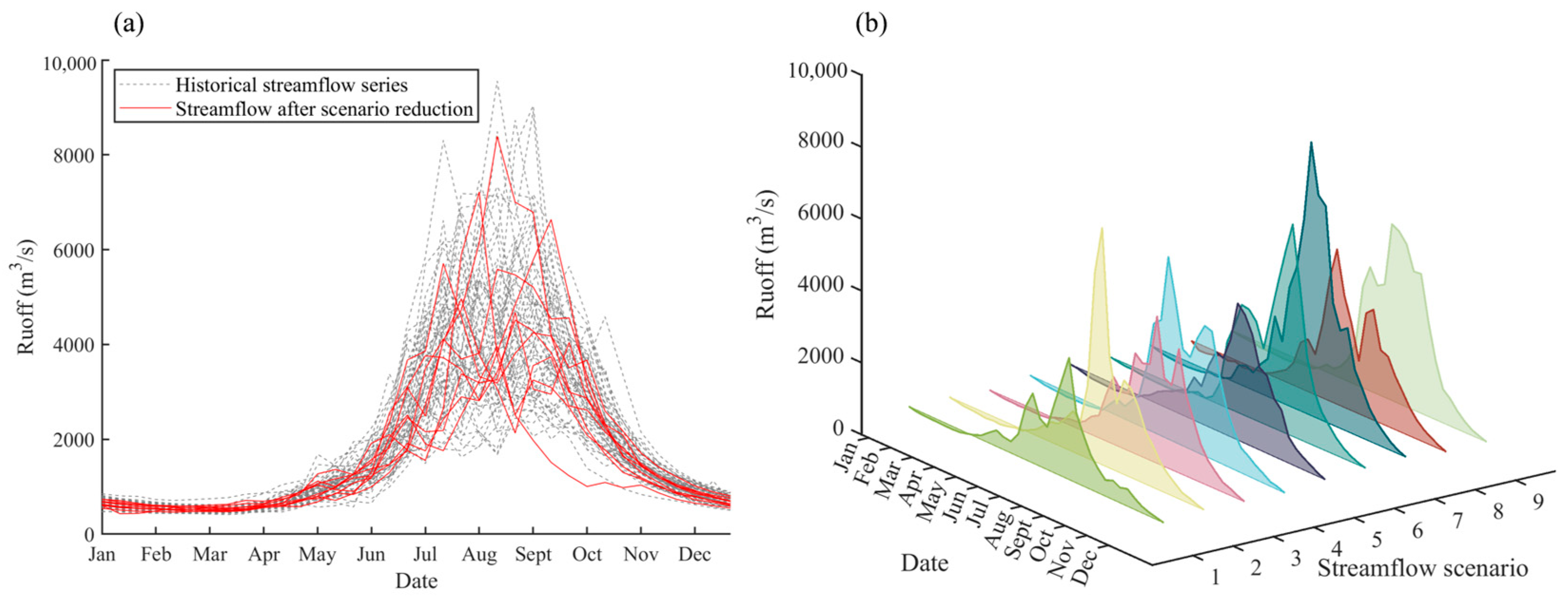
2.1. Streamflow and Scenario Reduction Module

The streamflow scenario reduction module including the DTW-SBR framework and evaluation indicators, is applied to acquire typical streamflow processes representing the natural hydrological regimes based on historical streamflow.

2.1.1. DTW-SBR Framework

The scenario reduction algorithm, named “backward reduction and forward selection”, was first proposed by Dupačová et al. [34] and then its computational efficiency was improved by Heitsch and Römisch [35]. By virtue of extracting processes with representative statistical characteristics, scenario reduction algorithms have been widely used in stochastic programming and generating time series of streamflow and hydro-wind-photovoltaic load [36,37,38,39]. Most scenario reduction algorithms generate reduced scenarios by minimizing Kantorovich or Euclidean distance among initial and reduced sequences, lacking matching accuracy [40]. Therefore, this study proposes a dynamic time warping scenario backward reduction (DTW-SBR) framework in which DTW, a well-known similarity measurement method for two sequences [41], is introduced to measure the similarity of scenarios in the scenario backward reduction (SBR). The processes of the DTW-SBR framework are as follows:

Step 1: Setting initial conditions. The initial scenarios of streamflow series with the total number of S are described as X = [X₁, X₂, …, X_s, …, X_S] with the corresponding probability P = [p₁, p₂, …, p_S], where the sth scenario X_s = [x(1)^s, x(2)^s, …, x(t)^s, …, x(T)^s]. Set the deleted number and scenarios as L and J, respectively, so the reserved scenarios are (X − J). Set the reduction iteration k = 1.

Step 2: Calculate the probabilistic DTW distance between X_i and X_j of the kth iteration as follows:

$$\left\{\begin{array}{l}{d}_{i,j}^{(k)}=\underset{{\mathit{X}}_j\notin {\mathit{J}}^{(k-1)}\cup \left({\mathit{X}}_i^k\right)}{\min }d\left({\mathit{X}}_i,{\mathit{X}}_j\right)\\ D_{i,j}^{(k)}=p_i^{(k)}\times d_{i,j}^{(k)}\end{array}\right.$$

(1)

where p_i^(k) represents the corresponding probability of the reduced scenario X_i in the kth iteration; D_i,j^(k) represents the probabilistic DTW distance between the reduced scenario X_i and the initial scenario X_j in the kth iteration; d_i,j^(k) represents the DTW distance, which can be calculated as follows:

Step 2.1: For two time series A = [a₁, a₂, …, a_i, …, a_m] and B = [b₁, b₂, …, b_j, …, b_n], where m and n are the lengths of two time series, respectively, the distance matrix W(i, j) can be calculated as follows:

$$W\left(i,j\right)=\left|a_i-b_j\right|$$

(2)

Step 2.2: Calculate the minimum accumulative distance from W(1, 1) to W(m, n), which is displayed in Figure 2 as follows:

$$\theta \left(i,j\right)=W\left(i,j\right)+\min \left[\theta \left(i-1,j\right),\theta \left(i,j-1\right),\theta \left(i-1,j-1\right)\right]$$

(3)

where θ(i, j) represents minimum accumulative distance, which can be calculated according to dynamic programing [42].

Step 3: Scenario reduction. Delete the scenario X_i^(k) with the minimum D_i,j^(k) from the reserved scenarios (X − J) and merge into J^(k−1), then J^(k) = J^(k−1) ∪ {X_i^(k)}. The probability p_i^k−1 of X_i^(k) is added to the probability p_j^k−1 of X_j^(k−1) among scenarios (X − J^(k−1)) with the corresponding minimum DTW distance, which can be calculated as follows:

$$p_j^k=p_j^{k-1}+p_i^{k-1}$$

(4)

Step 4: k = k + 1, then repeat Steps 2 and 3 until obtaining the streamflow scenarios X* = [X₁*, X₂*, …, X_s*, …, X_S−L*] with the corresponding probability P* = [p₁*, p₂*, …, p_S−L*].

2.1.2. Evaluation Indicators

This study adopts three evaluation indicators to measure the difference in degrees between streamflow scenarios and historical series for determining the appropriate number of scenario reduction, which are as follows: total mean deviation squared (TMDS), mean squared error (MSE) and total deviation of standard deviation (TDSD) [38].

(1) TMDS describes the deviation in the reduced streamflow scenarios’ weighted mean values from the historical streamflow series’ mean values. A low TMDS indicates the reduced streamflow scenarios have a good match with the historical streamflow series on mean values at different time periods. The TMDS for the kth streamflow scenario and historical streamflow series can be calculated as follows:

$$TMD{S}_k={\displaystyle \sum _{t=1}^T{\left[{\mu }_t^k-{\mu }_t^{\ast }\right]}^2}$$

(5)

$$\left\{\begin{array}{l}{\mu }_t^k={\displaystyle {\sum }_{m=1}^k{Q}^m\left(t\right)p^m}\\ {\mu }_t^{\ast }=\frac{{\displaystyle {\sum }_{y=1}^Y{R}_y\left(t\right)}}{Y}\end{array}\right.$$

(6)

where TMDS_k is the value of TMDS when the number of scenario reduction is k; μ_t^k and μ_t* are the weighted mean value of scenario streamflow and mean value of historical streamflow series at time t, respectively; Q^m(t) and p^m are the value of the mth streamflow scenario at time t and corresponding probability, respectively; R_y(t) is the value of historical streamflow of year y at time t; Y and T denote the total years and operation time periods, respectively.

(2) MSE is a common indicator for measuring the difference between two series using the Euclidean distance. The lower the MSE means the higher approaching degree between reduced streamflow scenarios and historical streamflow series. The MSE for the kth streamflow scenario and historical streamflow series can be calculated as follows:

$$MS{E}_k=\raisebox{1ex}{${\displaystyle {\sum }_{y=1}^Y\left\{{\displaystyle {\sum }_{t=1}^T{\left[R_y\left(t\right)-{\mu }_t^k\right]}^2}\right\}}$}\!\left/ \!\raisebox{-1ex}{$Y$}\right.$$

(7)

where MSE_k is the value of MSE when the number of scenario reduction is k.

(3) TDSD estimates the deviation in reduced streamflow scenarios’ standard deviation from the historical streamflow series’ standard deviation. The lower the TDSD means the reduced streamflow scenarios reproduce the features of extreme values of historical streamflow series. The TDSD for the kth streamflow scenario and historical streamflow series can be calculated as follows:

$$TDS{D}_k={\displaystyle {\sum }_{t=1}^T\left|{\sigma }_t^k-{\sigma }_y^{\ast }\right|}$$

(8)

$$\left\{\begin{array}{l}{\sigma }_t^k=\sqrt{{\displaystyle {\sum }_{m=1}^k{\left[Q^m\left(t\right)-{\mu }_t^k\right]}^2{p}^m}}\\ {\sigma }_y^{\ast }=\sqrt{\frac{{\displaystyle {\sum }_{y=1}^Y{\left[R_y\left(t\right)-{\mu }_t^{\ast }\right]}^2}}{Y-1}}\end{array}\right.$$

(9)

where, TDSD_k is the value of TDSD when the number of scenario reduction is k; σ_t^k and σ_y* represent standard deviation of the mth streamflow scenario and historical streamflow of year y, respectively.

The appropriate number of reduced streamflow scenarios can be determined through plotting curves of evaluation indicators with different ks.

2.2. Hydroregime-Hydroelectricity Operation Mode

2.2.1. Multi-Objective Functions

A hydroregime-hydroelectricity operation model is established to deal with two objectives: to minimize the deviation degrees of the hydrological regime at the downstream section (O1); to maximize the hydropower generation of reservoirs (O2). The multi-objective functions are formulated below.

O1: to minimize the deviation degrees of hydrological regimes at the downstream section,

$$f_1=\min {\displaystyle \sum _{y=1}^Y{\displaystyle \sum _{m=1}^k{\displaystyle \sum _{t=1}^T{\left[q^m\left(t\right)-q_y^{\ast }\left(t\right)\right]}^2{p}^m}}}$$

(10)

where q^m(t) represents the streamflow of the downstream section at time t of the mth reduced streamflow scenario; q_y*(t) represents the streamflow of the downstream section at time t of year y after the operation of reservoirs.

O2: to maximize the hydropower generation of reservoirs,

$$f_2=\max {\displaystyle \sum _{y=1}^Y{\displaystyle \sum _{t=1}^T{N}_{i,y}\left(t\right)\Delta t}}$$

(11)

where N_i,y(t) represents the hydropower output of the ith reservoir at time t of year y; Δt is the time interval of the operation period.

2.2.2. Constraints

(1) Water balance equation of reservoirs:

$$\left[Q_{i,y}^{\mathrm{in}}\left(t\right)-Q_{i,y}^{\mathrm{out}}\left(t\right)\right]\Delta t=V_{i,y}\left(t+1\right)-V_{i,y}\left(t\right)$$

(12)

where Q_i,yⁱⁿ(t) and Q_i,y^out(t) represent the inflow and outflow of the ith reservoir at time t of year y, respectively; V_i,y(t) represents the water storage of the ith reservoir at time t of year y.

(2) Water level limitation of reservoirs:

$$Z_{i,y}^{\min }\left(t\right)\le Z_{i,y}\left(t\right)\le Z_{i,y}^{\max }\left(t\right)$$

(13)

where Z_i,y(t) represents the water level of the ith reservoir at time t of year y; Z_i,y^min(t) and Z_i,y^max(t) represent the lower and upper water level limits of the ith reservoir at time t of year y, respectively.

(3) Hydropower output limitation:

$$N_{i,y}^{\min }\left(t\right)\le N_{i,y}\left(t\right)\le N_{i,y}^{\max }\left(t\right)$$

(14)

where N_i,y^min(t) and N_i,y^max(t) represent the lower and upper hydropower output limits of the ith reservoir at time t of year y, respectively.

(4) Outflow limitations of reservoirs:

$$Q_{i,y}^{\min }\left(t\right)\le Q_{i,y}^{\mathrm{out}}\left(t\right)\le Q_{i,y}^{\max }\left(t\right)$$

(15)

where Q_i,y^min(t) and Q_i,y^max(t) represent the minimum and maximum outflow of the ith reservoir at time t of year y, respectively.

(5) Start and end-of-operation water level limitation:

$$Z_{i,y}\left(1\right)=Z_{i,y}^{\mathrm{start}}{Z}_{i,y}\left(T+1\right)=Z_{i,y}^{\mathrm{end}}$$

(16)

where Z_i,y^start and Z_i,y^end represent the initial and end-of-operation water level of the ith reservoir of year y, respectively.

(6) Hydraulic connections:

$$Q_{i+1,y}^{\mathrm{in}}\left(t\right)=Q_{i,y}^{\mathrm{out}}\left(t\right)+\Delta q_{i+1,y}\left(t\right)$$

(17)

where Δq_i+1,y(t) represents the lateral inflow of the (i + 1)th reservoir at time t of year y.

2.3. Multi-Objective Optimization Method for Long-Term Operation

Generally, the outflow or water levels of each reservoir at each operation time period are selected as decision variables for solving the multi-objective operation model by multi-objective optimization algorithms [43]. However, for the long-term multi-objective operation problems of cascade reservoirs, the number of decision variables and solving difficulty increase greatly with the number of operation time periods and reservoirs rising [44]. For example, for a cascade-reservoirs system with M number of reservoirs and 10-day runoff of Y years, the number of decision variables can reach 36 (operation time periods of 10-day runoff for a year) × M × Y. It is hard for a single multi-objective optimization algorithm to solve the model if the number of reservoirs and years is too large.

Aimed at multi-objective optimization for the long-term operation of cascade reservoirs, this study proposes a “simulation-optimization” method which combines the long-term CO rules of reservoirs with the multi-objective optimization algorithm. The illustration of the reservoir’s long-term CO curve is shown in Figure 3. In Figure 3, the long-term CO curve of the reservoir is represented as time versus water level. The phases of long-term CO of reservoirs can be divided into four stages: the benefit-operation period (before t₁ and after t₄), drawdown-operation period (t₁~t₂), flood-control-operation period (t₂~t₃) and impoundment-operation period (t₃~t₄). In the benefit-operation period, the reservoir water levels are close to the normal water level for more hydropower generation. In the drawdown-operation period, the reservoir water levels decrease from the normal water level to the flood-limited one. In the flood-control-operation period, the reservoir water level maintains the flood-limited water level for reserving enough flood control capacity. In the impoundment-operation period, the reservoir water level increases gradually to the normal water level for meeting various purposes, including hydropower production, water supply and irrigation. When the long-term CO rule curve of the reservoir is determined, the reservoir outflow can be calculated according to the reservoir storage capacity curve and the water balance equation, which are listed below.

$$\left\{\begin{array}{l}V\left(t\right)=f_{zv}\left[Z\left(t\right)\right]\\ V\left(t+1\right)=f_{zv}\left[Z\left(t+1\right)\right]\\ Q^{\mathrm{out}}\left(t\right)=Q^{\mathrm{in}}\left(t\right)+\left[V\left(t\right)-V\left(t+1\right)\right]/\Delta t\end{array}\right.$$

(18)

where f_zv(*) is the reservoir storage capacity curve; V(t) and Z(t) are reservoir capacity and water level at time t, respectively; Qⁱⁿ(t) and Q^out(t) are the inflow and outflow of the reservoir at time t, respectively. The reservoir water level Z(t) can be determined according to the long-term CO curve of the reservoir and the reservoir inflow is the given value. So, the reservoir outflow can be calculated to obtain reservoir processes according to (18). That is to say, the reservoir outflow for each year can be simulated and the fitness values of multi-objectives can be calculated through the hydroregime-hydroelectricity operation model.

As for the multi-objective optimization algorithms, considering the fast convergence in obtaining the Pareto-front solutions with uniform distribution, the NSGA-II proposed by Deb et al. [45] has been widely applied in tackling the multi-objective operation of reservoirs, including hydropower production, flood defense, agricultural irrigation and water allocation [46,47,48], which has the ability to incorporate the simulation model of reservoir operation [49,50,51]. Therefore, this study incorporates the NSGA-II based on the multi-objective toolbox of MATLAB (MATLAB R2022b) into the long-term CO rule curves of reservoirs to acquire the Pareto-front solutions for synergistically optimizing the regulation of the cascade reservoirs from the perspectives of hydrological regimes and hydropower generation. The structure of long-term CO rule curves and NSGA-II is executed according to the following steps.

Step 1: Set up the NSGA-II parameters, including the population size NP, the maximum iteration K, the crossover rate p₁ and the mutation rate p₂.

Step 2: Set the iteration number k = 1 and randomly initialize the parent population P_k. Simulate the operation of cascade reservoirs according to the decision variables (reservoir outflow of each time period) and constraints (12)~(17), and calculate the fitness values of O1 and O2 by using the functions (10) and (11). Subsequently, sort each solution set of P_k using the fast non-dominated sorting method.

Step 3: Generate offspring population Q_k of size NP through the operators of selection, crossover and mutation.

Step 4: Integrate the P_k with Q_k to obtain R_k with the size of 2NP. Sort each solution set of R_k by the fast non-dominated sorting method, and calculate their crowding distances.

Step 5: Choose the new parent population P_k+1 from R_k. Then the offspring population Q_k+1 is also produced. Calculate the fitness values of O1 and O2 by using the functions (10) and (11). Then k = k + 1.

Step 6: Repeat Steps 4 and 5 until achieving termination conditions. Then the Pareto-front solutions are generated.

3. Materials

The Jinsha River Basin, which spans five provinces of China including Qinghai, Tibet, Sichuan, Yunnan and Guizhou, is located in the upper reach of the Yangtze River with a length of about 3500 km and a drainage area of over 45 × 10⁴ km². The upstream, midstream and downstream of the Jinsha River are demarcated by two hydrological stations, Shigu and Panzhihua, with mean annual runoffs of 444 × 10⁸ m³ and 538 × 10⁸ m³, respectively. The mean annual 10-day runoff at the Panzhihua hydrological station is displayed in Figure 4. The flood season of the midstream of the Jinsha River is from June to October, accounting for over 75% of the annual runoff.

Six large reservoirs (the characteristic information listed in

Table 1. Characteristic parameters of reservoirs in the middle reaches of the Jinsha River.

Reservoir	Dam Height (m)	Dead Water Level (m)	Flood-Limited Water Level (m)	Normal Water Level (m)	Minimum Outflow * (m3/s)	Regulating Storage (108 m3)	Total Storage (108 m3)	Installed Capacity (MW)
LY	155	1605	1605	1618	300	1.73	8.05	2400
AH	130	1492	1493.3	1504	350	2.38	8.85	2000
JAQ	160	1398	1410	1418	350	3.46	9.13	2400
LKK	119	1290	1289	1298	380	1.13	5.58	1800
LDL	140	1216	1212	1223	400	3.76	17.18	2160
GYY	159	1122.3	1122.3/1128.8	1134	439	5.55	22.50	3000

Note: * The reservoir minimum outflow is an indicator considering the maintenance environmental flow and the discharge corresponding to minimum hydropower output.

), Liyuan (LY), Ahai (AH), Jinanqiao (JAQ), Longkaikou (LKK), Ludila (LDL) and Guanyinyan (GYY), have been constructed in the middle reaches of the Jinsha River with a length of 563 km and a drainage area of 4.5 × 10⁴ km², which is displayed in Figure 5. The main purpose of these six reservoirs is hydropower generation, with also considering flood defense. According to Joint Operation Plan of Water Engineering in the Yangtze River Basin [52], the CO rule curves (shown in Figure 6) are used to guide the long-term operation of these six reservoirs. In Figure 6, for the LY, AH, JAQ, LKK and LDL reservoirs, during the periods from January to June and August to December, the reservoirs maintain the normal water levels to generate more hydropower and decline to the flood-limited water level in July to reserve flood control storage capacity for flood defense. For the GYY reservoir, except for reserving flood storage capacity in July, its water level also maintains at 1128.8 m from August to September for flood defense of the Panzhihua hydrological station.

A total of 13,608 datasets (=6 variables (inflows of 6 reservoirs) × 2268 time intervals (10-days runoff data of each reservoir from 1953 to 2015), 13,608 decision variables (=6 variables (outflow of 6 reservoirs) × 2268 time intervals)) and 13,608 constraints (=6 constraints in Equations (12)–(17) × 2268 time intervals) were collected for streamflow scenario reduction and the multi-objective operation of cascade reservoirs.

4. Results and Discussion

4.1. Streamflow Scenario Reduction

Three evaluation indicators (in Equations (5), (7) and (8)) are adopted to assess the proper number of scenario reduction. The results of TMDS, MSE and TDSD are shown in Figure 7. Figure 8 displays the historical and streamflow series and reduced streamflow scenarios of the Panzhihua hydrological station.

According to Figure 7, the values of TMDS, MSE and TDSD exhibit a downward trend in correlation with the increase in the number of scenario reduction. This indicates that the differences between the historical streamflow series and reduced streamflow scenarios become small. As the number of scenario reduction is gradually increased to nine, the values of TMDS, MSE and TDSD decline quickly. When the number of scenario reduction exceeds nine, the downward trends of these evaluation indicators increase slowly. This means the number nine can be considered as an abrupt point in trends of TMDS, MSE and TDSD for scenarios reduction. Therefore, the appropriate number of scenario reduction is set to nine.

Figure 8 shows nine streamflow scenarios are selected from the historical streamflow series of the Panzhihua hydrological station through the SBR-DTW framework. In Figure 8a, there are seasonal characteristics in the nine reduced scenarios. During the dry season (from January to April), the streamflow of the reduced scenarios is less than 1000 m³/s, while it increases quickly to over 4000 m³/s from May to September (the flood season) and then declines to less than 2000 m³/s after October. That is to say, the processes of the nine streamflow scenarios reflect intra-annual variability characteristics of the historical streamflow. In Figure 8b, for different streamflow scenarios, the flow processes during the period from January to April are similar, which are less than 1000 m³/s, while during the flood season (from May to September), the differences in flow processes are great. For some streamflow scenarios, such as Scenarios 2 and 7, the streamflow quickly rises to over 7000 m³/s in July. For some streamflow scenarios, such as Scenarios 1 and 3, the annual maximum streamflow occurring in August is less than 5000 m³/s.

Characteristic indicators including the annual maximum 10-day flow, annual minimum 10-day flow, time of annual maximum 10-day flow, annual runoff and probability (calculated by Equations (1)–(4)) are adopted to illustrate the differences in these nine streamflow scenarios in

Table 2. The characteristic indicators of the reduced streamflow scenarios.

Streamflow Scenario	Annual Maximum 10-Day Flow (m3/s)	Time of Annual Maximum 10-Day Flow	Annual Minimum 10-Day Flow (m3/s)	Annual Runoff (108 m3)	Probability (%)
1	3959	Mid-August	514	384	12.70
2	7219	Early August	475	500	6.35
3	4677	Late August	465	487	14.29
4	5709	Mid-July	550	566	14.29
5	4515	Late August	572	513	7.94
6	6636	Mid-September	531	610	11.11
7	8388	Mid-August	592	712	12.70
8	4965	Late July	431	515	9.52
9	5587	Mid-August	490	585	11.11

. Considering that the mean annual runoff of the Panzhihua hydrological station is 440 × 10⁸ m³, Scenario 1, with an annual runoff of 384 × 10⁸ m³, represents the dry flow year and its annual maximum flow is also obviously less than other scenarios. Scenarios 2, 3, 5 and 8, with annual runoffs ranging from 487 × 10⁸ m³ to 515 × 10⁸ m³, represent the normal flow years. It is noted that the annual maximum 10-day flow of Scenarios 3, 5 and 8 is no more than 5000 m³/s, but for Scenario 2, the annual maximum 10-day flow is over 7200 m³/s. This means more water volume is distributed in early August (occurrence time of the annual maximum 10-day flow) for Scenario 2. In addition, the annual runoff of Scenarios 4, 6, 7 and 9 ranges from 566 × 10⁸ m³ to 712 × 10⁸ m³, representing the wet flow years.

Overall, the nine reduced streamflow scenarios, including dry, normal and wet flow years, reflect the intra- and inter-annual variability of hydrological regimes at the Panzhihua hydrological station, which can be used for calculating the fitness values of O1 (as shown in Equation (10)) in the hydroregime-hydroelectricity operation model.

4.2. Optimization of the Two Objectives by NSGA-II

Based on the long-term 10-day runoff data from 1953 to 2015, the Pareto-front solutions of the hydroregime-hydroelectricity operation model obtained from the NSGA-II concerning the minimum deviation degrees of the hydrological regime at the Panzhihua hydrological station (O1) and the maximum hydropower generation of reservoirs (O2) are shown in Figure 9. Additionally, the values of these two objectives are calculated by the long-term CO rules, which are displayed in Figure 9 for comparison with the Pareto-front solutions.

In Figure 9, the O1 and O2 values of the long-term CO rules are 402,638 and 34,089 × 10⁸ kW·h, respectively. It is found that there is a competitive relationship between O1 and O2. O1 shows an increasing trend with the growth of O2, indicating that the improvement of O2 can diminish the benefit of O1 because runoff regulation of cascade reservoirs can increase hydropower generation while altering the natural hydrological regimes of the Panzhihua hydrological station. The point of the long-term CO rules stays far away from the Pareto-front solutions. This indicates that the Pareto-front solutions can synergistically boost the benefits of O1 and O2 compared to the long-term CO rules. According to the relative position of the point of the long-term CO rules and Pareto-front points in Figure 9, the distribution of the Pareto-front points can be partitioned into two zones, Zones I and II, and three typical schemes are acquired from the Pareto-front solutions, which are schemes A, B and C.

Table 3. The fitness values of O1 (the minimum deviation degrees of hydrological regime at the Panzhihua hydrological station) and O2 (the maximum hydropower generation of reservoirs) obtained from the long-term CO rules and typical schemes of the Pareto-front solutions.

Scheme	O1	O2 (108 kW·h)	Improvement rate of O1 (%) *	Improvement rate of O2 (%) **
Long-term CO rules (Benchmark)	402,638	34,089	/	/
Scheme A	378,673	35,841	5.95	5.14
Scheme B	361,678	34,083	10.17	0.00
Scheme C	360,326	32,837	10.51	−3.67

Note: * Improvement rate of O1 (%) = $\frac{\mathrm{O}1 \mathrm{value}\left\{\mathrm{Long}\text{-}\mathrm{term} \mathrm{CO} \mathrm{rules}\right\}-\mathrm{O}1 \mathrm{value}\left\{\mathrm{Parto}\text{-}\mathrm{front} \mathrm{solution}\right\}}{\mathrm{O}1 \mathrm{value}\left\{\mathrm{Long}\text{-}\mathrm{term} \mathrm{CO} \mathrm{rules}\right\}}\times 100\%$; ** Improvement rate of O2 (%) = $\frac{\mathrm{O}2 \mathrm{value}\left\{\mathrm{Parto}\text{-}\mathrm{front} \mathrm{solution}\right\}-\mathrm{O}2 \mathrm{value}\left\{\mathrm{Long}\text{-}\mathrm{term} \mathrm{CO} \mathrm{rules}\right\}}{\mathrm{Fitness} \mathrm{value}\left\{\mathrm{Long}\text{-}\mathrm{term} \mathrm{CO} \mathrm{rules}\right\}}\times 100\%.$

lists the values of O1 and O2 from both the long-term CO rules and the three typical schemes of the Pareto-front solutions.

In Zone I of Figure 9, the O1 and O2 values of the Pareto-front solutions are both smaller than those of the long-term CO rules, which means that the streamflow processes at the Panzhihua hydrological station using the operation schemes from Zone I of the Pareto-front solutions are closer to the natural hydrological regimes compared to the long-term CO rules, but the hydropower generation of six reservoirs is diminished. In Zone II of Figure 9, the O1 (O2) values of the Pareto-front solutions are smaller (larger) than those of the long-term CO rule, which implies that the operation schemes from Zone II can simultaneously optimize the benefits of O1 and O2, as compared to the long-term CO rules.

The three typical schemes, A, B and C, in Figure 9 represent the inclination to be the situation dominated by different objectives. Scheme A, with the largest hydropower generation of 35,841 × 10⁸ kw·h (as listed in Table 3), tends to be the Pareto-front solution completely dominated by O2. Compared to the long-term CO rules, O1 and O2 using the Scheme A are improved by 5.94% and 5.14%, respectively. Scheme B, with the hydropower generation of 34,083 kw·h (as listed in Table 3), equal to the long-term CO rules, is inclined to be the Pareto-front solution decreasing the deviation degrees of the hydrological regime at the Panzhihua hydrological station without reducing the benefits of the hydropower generation. For O1, Scheme B offers a deviation degree of 10.17% less than that of the long-term CO rules. Scheme C, with the minimum deviation degrees of the hydrological regime at the Panzhihua hydrological station (360,326 as listed in Table 3), seems to be the Pareto-front solution completely dominated by O1. Scheme C can improve O1 by 10.51%, while reducing O2 by 3.67%, as compared to the long-term CO rules.

All in all, the Pareto-front solutions, especially in Zone II of Figure 9, can synergistically optimize O1 and O2, as compared to the long-term CO rules. The smaller O1 represents that the reservoir outflow processes are similar to the natural streamflow, which means mitigating the alteration of the reservoir operation on the natural hydrological regimes.

4.3. Analysis of Reservoir Operation Schemes

The long-term CO rules and Schemes A to C for each reservoir in the middle reaches of the Jinsha River are displayed in Figure 10. The total hydropower generation of different operation schemes from 1953 to 2015 for each reservoir is listed in

Table 4. The total hydropower generation of the long-term CO rules and Schemes A to C from 1953 to 2015 for each reservoir in the middle reaches of the Jinsha River.

Reservoir	Long-Term CO Rule (108 kw·h)	Scheme A		Scheme B		Scheme C
		Hydropower Generation (108 kw·h)	Increase Rate (%) *	Hydropower Generation (108 kw·h)	Increase Rate (%) *	Hydropower Generation (108 kw·h)	Increase Rate (%) *
LY	5742	5910	2.93	5426	−5.51	5271	−8.21
AH	5414	5420	0.10	5211	−3.75	5161	−4.68
JAQ	6328	6690	5.72	6295	−0.53	5914	−6.55
LKK	4470	4700	5.14	4361	−2.45	4043	−9.56
LDL	5156	5480	6.29	5428	5.28	5274	2.29
GYY	6979	7641	9.48	7362	5.49	7176	2.82

Note: * Increase rate (%) = $\frac{\mathrm{Hydropower} \mathrm{generation}\left\{\mathrm{Schemes} \mathrm{A} \mathrm{to} \mathrm{C}\right\}-\mathrm{Hydropower} \mathrm{generation}\left\{\mathrm{long}\text{-}\mathrm{term} \mathrm{CO} \mathrm{rules}\right\}}{\mathrm{Hydropower} \mathrm{generation}\left\{\mathrm{long}\text{-}\mathrm{term} \mathrm{CO} \mathrm{rules}\right\}}\times 100\%.$

.

In Figure 10a–d, when using Scheme C, the water levels of the LY, AH, JAQ and LKK reservoirs decline to near reservoir dead water levels before late April and maintain low water levels until late September. In addition, the changing characteristics of water levels of these reservoirs using Scheme B are similar to those using Scheme C. This is because the implementation of the concentrated drawdown or impoundment-operation of cascade reservoirs may induce notable alterations in the hydrological regimes of the Panzhihua hydrological station from June to September, which is averse to the O1 benefit. The operation processes of these six cascade reservoirs using Scheme A show fluctuation trends during the periods from January to June. Since the inflow of the reservoirs before May is not very large, the fluctuation of reservoir water levels means properly increasing the reservoir outflow to enhance hydropower generation. In addition, the operation processes of the LY, AH, LKK and GYY reservoirs during periods from August to December (shown in Figure 10a,b,d,f) are the same as those of these reservoirs using the long-term CO rules.

In Table 4, the LDL and GYY reservoirs’ total hydropower generation of Schemes A to C from 1953 to 2015 is 2.29%~9.48% larger than that of the long-term CO rules. When using Schemes B and C, the hydropower generation of the LY, AH, JAQ and LKK reservoirs is 0.53%~9.56% less than that of the long-term CO rules since their water levels are lower than those using the long-term CO rules during the periods from April to September.

On the whole, Scheme A seems to be a recommended operation solution for simultaneously improving O1 and O2 by over 5% (listed in Table 3). The total hydropower generation of each reservoir using Scheme A from 1953 to 2015 is 0.1%~9.48% (listed in Table 4) larger than that using the long-term CO rules. According to Schemes B and C, in order to mitigate the deviation in the hydrological regime at the Panzhihua hydrological station, the water levels of the LY, AH, JAQ and LKK reservoirs should be reduced to the low values prior to July and the reservoir filling time should be postponed until after the end of September.

5. Conclusions

The construction and operation of cascade reservoirs is one of efficient measures for meeting socio-economic needs and resisting natural hazards, while altering the natural hydrological regimes. This study proposes the DTW-SBR framework for the purpose of streamflow scenario reduction to offer the ecological optimization objective, and develops a multi-objective ecological long-term operation model that is solved by the NSGA-II based on the reservoir long-term CO rules to achieve the maximum hydropower generation of cascade reservoirs (O1) and the minimum deviation degrees of hydrological regimes at the Panzhihua hydrological station (O2). The main findings are summarized below.

(1) Nine streamflow scenarios are extracted from the historical streamflow series through the DTW-SBR framework. These nine streamflow scenarios, including dry, normal and wet flow years, reflect the intra- and inter-annual variability of natural hydrological regimes at the Panzhihua hydrological station. They are regarded as benchmarks for calculating O1 values in the multi-objective optimal operation model.

(2) There is a competitive relationship between O1 and O2, which indicates that enhancing O2 leads to increasing O1, and vice vera. Compared to the long-term CO rules, the operation schemes in Zone II of Pareto-front solutions can simultaneously optimize O1 (with improvement rates from 5.95% to 10.17%) and O2 (with improvement rates from 0% to 5.14%).

(3) Three operation schemes, A, B and C, from the Pareto-front solutions represent an inclination to be the situation dominated by different objectives. Compared to the long-term CO rules, Scheme A increases the hydropower generation of each reservoir by 6 × 10⁸ kw·h to 662 × 10⁸ kw·h (corresponding improvement rate of 0.1% to 9.48%), while reducing O1 by 5.95%. Scheme B reduces O1 by 10.17% without decreasing O2, while Scheme C achieves the minimum O1 of 360,326 (corresponding improvement rate of 10.51%) with diminishing O2 by 3.67%, as compared to the long-term CO rules. Overall, Scheme A is a recommended operation solution for simultaneously improving O1 and O2.

The results indicate that the proposed multi-objective ecological long-term operation model could boost the synergistic benefits of two objectives in cascade reservoirs in the middle reaches of the Jinsha River. Schemes A, B and C, obtained from the Pareto-front solutions, could reveal the patterns of reservoir water levels for the long-term operation of improving hydropower generation and restoring hydrological regimes. Since the established model consists of the deterministic objective functions and constraints and the streamflow are historical observed data, the limitation of this study lies in its failure to consider uncertainty. In addition, the riverine water quality is also an indicator relating to riverine ecology. Therefore, there must be research on exploring relationships between the water quality and the riverine ecology in the future. The multi-objective ecological long-term operation model can be integrated with hydrologic forecasting information to explore the impact of the uncertainty of reservoir inflow on multi-objective operation.

References

1. Zhang, X.; Dong, Q.; Costa, V.; Wang, X. A hierarchical Bayesian model for decomposing the impacts of human activities and climate change on water resources in China. Sci. Total Environ. 2019, 665, 836–847. [Google Scholar] [CrossRef] [PubMed]
2. Wu, Z.; Mei, Y.; Chen, J.; Hu, T.; Xiao, W. Attribution analysis of dry season runoff in the Lhasa River using an extended hydrological sensitivity method and a hydrological model. Water 2019, 11, 1187. [Google Scholar] [CrossRef]
3. Xiong, F.; Guo, S.; Liu, P.; Xu, C.Y.; Zhong, Y.; Yin, J.; He, S. A general framework of design flood estimation for cascade reservoirs in operation period. J. Hydrol. 2019, 577, 124003. [Google Scholar] [CrossRef]
4. Zhang, H.; Chang, J.; Gao, C.; Wu, H.; Wang, Y.; Lei, K.; Long, R.; Zhang, L. Cascade hydropower plants operation considering comprehensive ecological water demands. Energy Convers. Manag. 2019, 180, 119–133. [Google Scholar] [CrossRef]
5. Javadinejad, S.; Ostad-Ali-Askari, K.; Jafary, F. Using simulation model to determine the regulation and to optimize the quantity of chlorine injection in water distribution networks. Model. Earth Syst. Environ. 2019, 5, 1015–1023. [Google Scholar] [CrossRef]
6. Ding, Z.; Fang, G.; Wen, X.; Tan, Q.; Huang, X.; Lei, X.; Tian, Y.; Quan, J. A novel operation chart for cascade hydropower system to alleviate ecological degradation in hydrological extremes. Ecol. Model. 2018, 384, 10–22. [Google Scholar] [CrossRef]
7. Ding, Z.; Fang, G.; Wen, X.; Tan, Q.; Lei, X.; Liu, Z.; Huang, X. Cascaded hydropower operation chart optimization balancing overall ecological benefits and ecological conservation in hydrological extremes under climate change. Water Resour. Manag. 2020, 34, 1231–1246. [Google Scholar] [CrossRef]
8. Nafchi, R.F.; Vanani, H.R.; Pashaee, K.N.; Brojeni, H.S.; Ostad-Ali-Askari, K. Investigation on the effect of inclined crest step pool on scouring protection in erodible river beds. Nat. Hazards 2022, 110, 1495–1505. [Google Scholar] [CrossRef]
9. Zhu, D.; Mei, Y.; Ben, Y.; Xu, X. Inter-and intra-annual trend analysis of water level and flow in the middle and lower reaches of the Ganjiang River, China. Hydrol. Sci. J. 2020, 65, 2128–2141. [Google Scholar] [CrossRef]
10. Ostad-Ali-Askari, K.; Ghorbanizadeh Kharazi, H.; Shayannejad, M.; Zareian, M.J. Effect of management strategies on reducing negative impacts of climate change on water resources of the Isfahan–Borkhar aquifer using MODFLOW. River Res. Appl. 2019, 35, 611–631. [Google Scholar] [CrossRef]
11. Yazdian, H.; Zahraie, B.; Jaafarzadeh, N. Multi—Objective Reservoir Operation Optimization by Considering Ecosystem Sustainability and Ecological Targets. Water Resour. Manag. 2024, 38, 881–892. [Google Scholar] [CrossRef]
12. Zhu, D.; Zhou, Y.; Guo, S.; Chang, F.J.; Lin, K.; Deng, Z. Exploring a multi-objective optimization operation model of water projects for boosting synergies and water quality improvement in big river systems. J. Environ. Manag. 2023, 345, 118673. [Google Scholar] [CrossRef] [PubMed]
13. Castelletti, A.; Pianosi, F.; Soncini-Sessa, R. Water reservoir control under economic, social and environmental constraints. Automatica 2008, 44, 1595–1607. [Google Scholar] [CrossRef]
14. Yin, X.; Yang, Z.; Yang, W.; Zhao, Y.; Chen, H. Optimized reservoir operation to balance human and riverine ecosystem needs: Model development, and a case study for the Tanghe reservoir, Tang river basin, China. Hydrol. Process. 2010, 24, 461–471. [Google Scholar] [CrossRef]
15. Li, Y.; Lin, J.; Liu, Y.; Yao, W.; Zhang, D.; Peng, Q.; Qian, S. Refined operation of cascade reservoirs considering fish ecological demand. J. Hydrol. 2022, 607, 127559. [Google Scholar] [CrossRef]
16. Lu, X.; Wang, X.; Ban, X.; Singh, V.P. Considering ecological flow in multi-objective operation of cascade reservoir systems under climate variability with different hydrological periods. J. Environ. Manag. 2022, 309, 114690. [Google Scholar] [CrossRef] [PubMed]
17. Ai, Y.; Ma, Z.; Xie, X.; Huang, T.; Cheng, H. Optimization of ecological reservoir operation rules for a northern river in China: Balancing ecological and socio-economic water use. Ecol. Indic. 2022, 138, 108822. [Google Scholar] [CrossRef]
18. Feng, Z.K.; Niu, W.J.; Cheng, C.T. Optimization of hydropower reservoirs operation balancing generation benefit and ecological requirement with parallel multi-objective genetic algorithm. Energy 2018, 153, 706–718. [Google Scholar] [CrossRef]
19. Jager, H.I.; Smith, B.T. Sustainable reservoir operation: Can we generate hydropower and preserve ecosystem values? River Res. Appl. 2008, 24, 340–352. [Google Scholar] [CrossRef]
20. Cioffi, F.; Gallerano, F. Multi-objective analysis of dam release flows in rivers downstream from hydropower reservoirs. Appl. Math. Model. 2012, 36, 2868–2889. [Google Scholar] [CrossRef]
21. Chen, W.; Olden, J.D. Designing flows to resolve human and environmental water needs in a dam-regulated river. Nat. Commun. 2017, 8, 2158. [Google Scholar] [CrossRef] [PubMed]
22. Saadatpour, M.; Afshar, A.; Solis, S.S. Surrogate-based multiperiod, multiobjective reservoir operation optimization for quality and quantity management. J. Water Resour. Plan. Manag. ASCE 2020, 146, 04020053. [Google Scholar] [CrossRef]
23. Yu, L.; Wu, X.; Wu, S.; Jia, B.; Han, G.; Xu, P.; Dai, J.; Zhang, Y.; Wang, F.; Yang, Q.; et al. Multi-objective optimal operation of cascade hydropower plants considering ecological flow under different ecological conditions. J. Hydrol. 2021, 601, 126599. [Google Scholar] [CrossRef]
24. Jordan, S.; Quinn, J.; Zaniolo, M.; Giuliani, M.; Castelletti, A. Advancing reservoir operations modelling in SWAT to reduce socio-ecological tradeoffs. Environ. Modell. Softw. 2022, 157, 105527. [Google Scholar] [CrossRef]
25. Richter, B.D.; Baumgartner, J.V.; Powell, J.; Braun, D.P. A method for assessing hydrologic alteration within ecosystems. Conserv. Biol. 1996, 10, 1163–1174. [Google Scholar] [CrossRef]
26. Bunn, S.E.; Arthington, A.H. Basic principles and ecological consequences of altered flow regimes for aquatic biodiversity. Environ. Manag. 2002, 30, 492–507. [Google Scholar] [CrossRef]
27. Yan, M.; Fang, G.H.; Dai, L.H.; Tan, Q.F.; Huang, X.F. Optimizing reservoir operation considering downstream ecological demands of water quantity and fluctuation based on IHA parameters. J. Hydrol. 2021, 600, 126647. [Google Scholar] [CrossRef]
28. Poff, N.L.; Allan, J.D.; Bain, M.B.; Karr, J.R.; Prestegaard, K.L.; Richter, B.D.; Sparks, R.E.; Stromberg, J.C. The natural flow regime. Bioscience 1997, 47, 769–784. [Google Scholar] [CrossRef]
29. Gao, Y.; Vogel, R.M.; Kroll, C.N.; Poff, N.L.; Olden, J.D. Development of representative indicators of hydrologic alteration. J. Hydrol. 2009, 374, 136–147. [Google Scholar] [CrossRef]
30. Zhang, Q.; Gu, X.; Singh, V.P.; Chen, X. Evaluation of ecological instream flow using multiple ecological indicators with consideration of hydrological alterations. J. Hydrol. 2015, 529, 711–722. [Google Scholar] [CrossRef]
31. Mohammed, H.; Hansen, A.T. Spatial heterogeneity of low flow hydrological alterations in response to climate and land use within the Upper Mississippi River basin. J. Hydrol. 2024, 632, 130872. [Google Scholar] [CrossRef]
32. Avesani, D.; Zanfei, A.; Di Marco, N.; Galletti, A.; Ravazzolo, F.; Righetti, M.; Majone, B. Short-term hydropower optimization driven by innovative time-adapting econometric model. Appl. Energy 2022, 310, 118510. [Google Scholar] [CrossRef]
33. Ahmad, S.K.; Hossain, F. Forecast-informed hydropower optimization at long and short-time scales for a multiple dam network. J. Renew. Sustain. Energy 2020, 12, 014501. [Google Scholar] [CrossRef]
34. Dupačová, J.; Gröwe-Kuska, N.; Römisch, W. Scenario reduction in stochastic programming. Math. Program. 2003, 95, 493–511. [Google Scholar] [CrossRef]
35. Heitsch, H.; Römisch, W. Scenario reduction algorithms in stochastic programming. Comput. Optim. Appl. 2003, 24, 187–206. [Google Scholar] [CrossRef]
36. Heitsch, H.; Römisch, W. Scenario tree modeling for multistage stochastic programs. Math. Program. 2009, 118, 371–406. [Google Scholar] [CrossRef]
37. Li, J.; Lan, F.; Wei, H. A scenario optimal reduction method for wind power time series. IEEE Trans. Power Syst. 2015, 31, 1657–1658. [Google Scholar] [CrossRef]
38. Li, J.; Zhu, F.; Xu, B.; Yeh, W.W.G. Streamflow scenario tree reduction based on conditional Monte Carlo sampling and regularized optimization. J. Hydrol. 2019, 577, 123943. [Google Scholar] [CrossRef]
39. Yin, Y.; Liu, T.; He, C. Day-ahead stochastic coordinated scheduling for thermal-hydro-wind-photovoltaic systems. Energy 2019, 187, 115944. [Google Scholar] [CrossRef]
40. Li, Z.; Zhang, F.; Nie, F.; Li, H.; Wang, J. Speed up dynamic time warping of multivariate time series. J. Intell. Fuzzy Syst. 2019, 36, 2593–2603. [Google Scholar] [CrossRef]
41. Berndt, D.J.; Clifford, J. Using dynamic time warping to find patterns in time series. In Proceedings of the 3rd International Conference on Knowledge Discovery and Data Mining, Seattle, WA, USA, 31 July–1 August 1994; pp. 359–370. [Google Scholar]
42. Yakowitz, S. Dynamic programming applications in water resources. Water Resour. Res. 1982, 18, 673–696. [Google Scholar] [CrossRef]
43. Yang, Z.; Yang, K.; Wang, Y.; Su, L.; Hu, H. Long-term multi-objective power generation operation for cascade reservoirs and risk decision making under stochastic uncertainties. Renew. Energy 2021, 164, 313–330. [Google Scholar] [CrossRef]
44. Zhang, W.; Liu, P.; Chen, X.; Wang, L.; Ai, X.; Feng, M.; Liu, D.; Liu, Y. Optimal operation of multi-reservoir systems considering time-lags of flood routing. Water Resour. Manag. 2016, 30, 523–540. [Google Scholar] [CrossRef]
45. Deb, K.; Agrawal, S.; Pratap, A.; Meyarivan, T. A fast elitist non-dominated sorting genetic algorithm for multi-objective optimization: NSGA-II. In Parallel Problem Solving from Nature PPSN VI, Proceedings of the 6th International Conference, Paris, France, 18–20 September 2000; Springer: Berlin/Heidelberg, Germany, 2000; Proceedings 6. [Google Scholar]
46. Hojjati, A.; Monadi, M.; Faridhosseini, A.; Mohammadi, M. Application and comparison of NSGA-II and MOPSO in multi-objective optimization of water resources systems. J. Hydrol. Hydromech. 2018, 66, 323–329. [Google Scholar] [CrossRef]
47. Wu, L.; Bai, T.; Huang, Q.; Wei, J.; Liu, X. Multi-objective optimal operations based on improved NSGA-II for Hanjiang to Wei River Water Diversion Project, China. Water 2019, 11, 1159. [Google Scholar] [CrossRef]
48. He, W.; Ma, C.; Zhang, J.; Lian, J.; Wang, S.; Zhao, W. Multi-objective optimal operation of a large deep reservoir during storage period considering the outflow-temperature demand based on NSGA-II. J. Hydrol. 2020, 586, 124919. [Google Scholar] [CrossRef]
49. Gonzalez, J.M.; Tomlinson, J.E.; Harou, J.J.; Ceseña, E.A.M.; Panteli, M.; Bottacin-Busolin, A.; Hurford, A.; Olivares, M.A.; Siddiqui, A.; Erfani, T.; et al. Spatial and sectoral benefit distribution in water-energy system design. Appl. Energy 2020, 269, 114794. [Google Scholar] [CrossRef]
50. He, Y.; Guo, S.; Zhou, Y.; Zhu, D.; Chen, H.; Xiong, L.; Liu, J.; Xu, C.Y. Boosting hydropower generation of mixed reservoirs for reducing carbon emissions by using a simulation–optimization framework. Hydrol. Res. 2024, 55, 144–160. [Google Scholar] [CrossRef]
51. Zhu, D.; Chen, H.; Zhou, Y.; Xu, X.; Guo, S.; Chang, F.J.; Xu, C.Y. Exploring a multi-objective cluster-decomposition framework for optimizing flood control operation rules of cascade reservoirs in a river basin. J. Hydrol. 2022, 614, 128602. [Google Scholar] [CrossRef]
52. Joint Operation Plan of Water Engineering in the Yangtze River Basin. Changjiang Water Resources Commission of the Ministry of Water Resources; Joint Operation Plan of Water Engineering in the Yangtze River Basin: Wuhan, China, 2023. [Google Scholar]
Figure 1. Flowchart of the synergistic optimization of hydrological regime and hydroelectricity including (a) streamflow scenario reduction module; (b) hydroregime-hydroelectricity operation model; (c) multi-objective optimization method for long-term operation.
Water 16 01849 g001
Figure 2. The sketch of warping path of two time series.
Water 16 01849 g002
Figure 3. The sketch of long-term CO rule curves of reservoirs.
Water 16 01849 g003
Figure 4. The mean annual 10-day runoff at the Panzhihua hydrological station.
Water 16 01849 g004
Figure 5. Locations and generalized diagram of reservoirs in the middle reaches of the Jinsha River.
Water 16 01849 g005
Figure 6. Conventional operation rule curves of the six reservoirs in the middle reaches of the Jinsha River.
Water 16 01849 g006
Figure 7. The changes in TMDS, MSE and TDSD with increase in the number of scenario reduction.
Water 16 01849 g007
Figure 8. The historical streamflow series and reduced streamflow scenarios at the Panzhihua hydrological station. (a) the comparison of historical streamflow series and reduced streamflow scenarios with 10-day runoff; (b) the streamflow series of 9 scenarios after scenario reduction.
Water 16 01849 g008
Figure 9. The Pareto-front concerning the minimum deviation degrees of hydrological regime at the Panzhihua hydrological station (O1) and the maximum hydropower generation of reservoirs (O2).
Water 16 01849 g009
Figure 10. The operation processes of the long-term CO rules and Schemes A to C of six reservoirs in the middle reaches of the Jinsha River. (a) The operation schemes of the LY reservoir. (b) The operation schemes of the AH reservoir. (c) The operation schemes of the JAQ reservoir. (d) The operation schemes of the LKK reservoir. (e) The operation schemes of the LDL reservoir. (f) The operation schemes of the GYY reservoir.
Water 16 01849 g010