Predicting Water Inflow in Tunnel Construction: A Fracture Network Model with Non-Darcy Flow Considerations

Abstract

Fractures are widely distributed in karst areas, and when flow rates are high, they exhibit complex nonlinear behavior that cannot be accurately described by Darcy’s law. In this work, a hydro-mechanical coupling model based on a discrete fracture network is proposed to predict tunnel water inflow, accounting for the impact of non-Darcy flow. The model’s feasibility has been validated by comparing it with experimental results and the field measurements of flow rates at the Bodaoling Tunnel in Guizhou, China. The results show that Darcy flow tends to overestimate water inflow by approximately 25% compared to non-Darcy flow. The non-Darcy effect grows with the increase in initial fracture width and empirical constant q. When q exceeds 8.77 × 10⁻⁶, the growth rate of the Forchheimer number along the fracture width slowed down, and the inhibitory effect of non-Darcy flow on flow became gentle. Additionally, in a complex fracture network, the inflow rate limited by non-Darcy flow at one point drives the water flow through a connect fracture to another point, which increases the difficulty in water inflow prediction. This work highlights the importance of non-Darcy flow and fracture networks when accurately predicting water inflow in tunnels.

1. Introduction

Diverse structures in karst areas, such as fractures, karrens, and karst caves, provide abundant access for groundwater to tunnel. This heightened connectivity increases the risk of water inflow and mud outbursts during tunnel construction, potentially threating the safety of on-site personnel [1,2,3,4,5]. The water inflow is a significant issue for tunnel construction in water-rich karst regions. Overestimating water inflow can lead to overly conservative drainage plans [6], whereas underestimation may lead to seepage, mud, and water inrush [7,8,9]. Therefore, an accurate estimation of water inflow into the tunnel is indispensable for tunnel construction in water-rich karst regions [10,11,12].

The prediction of water inflow during tunnel construction has been extensively researched using theoretical, experimental, and numerical methods [1]. Goodman initially derived a steady-state analytical equation to predict water inflow into circular tunnels [13]. Building upon this, Moon and Fernandez proposed an estimation method for groundwater inflow that accounts for water table drawdown in fractured rock masses [14]. In addition, various analytic formulas such as the mirror method [15], the shaft method [16], and the conformal transformation method [17] have been consistently proposed based on Darcy’s Law. These formulas are user-friendly, allowing for quick calculations and reduced reliance on parameters. They can be flexibly applied to a variety of geological conditions. However, the assumptions and simple boundaries of these theoretical solutions limit their application to addressing complex engineering problems. Based on model experiment data, Sato and Iizawa established an unsteady flow formula for predicting stable water inflow [18]. Shi et al. experimentally studied the non-Darcy flow behavior in granular limestone with different porosities, concluding that greater porosity leads to higher Forchheimer numbers, representing non-Darcy flow effects [19]. However, the model size of these experiments may not be completely consistent with the actual engineering scenarios.

In comparison with theoretical and experimental methods, numerical methods show obvious advantages in addressing complex field-scale problems. A large number of numerical methods have been used to predict water inflow into tunnels with higher precision. Nikvar Hassani et al. applied an equivalent porous media model to study the influence of model dimensions on water inflow into a tunnel, finding that larger model sizes yield more accurate predictions [20]. Zhang et al. applied a dual-permeability numerical model to investigate the influence of water pressure while considering anisotropic features, including fracture dip angle, and the results showed that increasing water pressure and decreasing fracture spacing led to increased water inflow [21].

Empirical formulas are commonly utilized in engineering specifications for predicting water inflow [22]. Based on geological and hydrological data within the project, the empirical formula can efficiently calculate water inflow in a wide range of tunnels. This calculation provides a foundation for the design and construction of drainage facilities. Based on the geological and hydrological conditions of Nanshan Tunnel, Jin et al. calculated water inflow using three empirical formulas: the groundwater runoff modulus method, the atmosphere precipitation infiltration method, and the groundwater dynamics method. After comparing the monitoring data, it was concluded that the groundwater dynamics method is the most suitable for the Nanshan Tunnel [23]. Zhang et al. compared the advantages and disadvantages of the groundwater runoff modulus method and the water balance method. They utilized an empirical formula and a support vector regression model to successfully forecast the distribution of a wide range of karst regions [24].

These studies have primarily focused on the mechanism and prediction methods of water inflow based on Darcy’s law, which is not sufficient to describe the nonlinear flow behavior of fluids with inertia effects. Notably, studies by Quinn et al., Lee et al., and Chen et al. have experimentally demonstrated strong nonlinear flow characteristics in rough fractures at specific velocities [25,26,27]. Zhou et al. developed a semi-empirical model based on numerical results and a parameter integration method to analytically predict water inflow in tunnels under non-Darcy flow regimes [28]. Their research highlighted the idea that ignoring the non-Darcy effect leads to increased errors in proportion to the inflow rate. Liu et al. introduced a nonlinear Forchheimer law to develop a semi-empirical model to predict the inflow under a stationary state, and a statistical analysis of 59 practical engineering cases found that ignoring the non-Darcy effect exaggerates the water inflow and influences the radius [29].

In karst areas, fractures serve as predominant channels for groundwater flow [30,31]. Huang et al. studied the impact of different fracture connectivity rates on groundwater flow, indicating that groundwater primarily flows through fractures with higher permeability [32]. Li et al. have proved that the fracture network has an important effect on the water inflow in a tunnel, and they analyzed the impact of factors such as fracture density, incline angle, stress anisotropy, and initial fracture width on inflow rates during tunnel construction [1]. Farhadian et al. have evaluated the impact of different model parameters, such as tunnel radius, groundwater level, joint spacing, joint dip/dip direction, and fracture width on the optimum model extent [33]. They presented an optimum model extent chart about the tunnel depth under the groundwater level, tunnel radius, and joint spacing. Based on the structural plane detection data of the study area, Shi et al. constructed a three-dimensional fracture network seepage model using the Monte Carlo algorithm and verified the model’s usability in the water surge simulation of Yue Long Men Tunnel [34]. These studies demonstrate that taking non-Darcy flow into account can lead to more accurate predictions of water inflow in tunnels. Meanwhile, the impact of non-Darcy flow on water utilization is more intricate. The current formula describing fluid nonlinearity needs to be expanded in order to achieve more stable and reliable calculation results.

The preceding studies on water inflow prediction in fractured aquifer tunnels have shown limited exploration of fracture distribution in the surrounding rock and the impact of the non-Darcy effect on tunnel water inflow. Further research in this area is essential.

This study introduces an equivalent fracture network model that incorporates non-Darcy flow and fracture network considerations, with the aim of enhancing the accuracy of tunnel water inflow predictions. An important advancement from previous models is the inclusion of fracture deformation and non-Darcy flow within fractures as part of the hydro-mechanical coupling framework [12,32,35]. In order to comprehensively depict the relationship between fractures and water inflow, the fracture network is reconstructed as realistically as possible according to the observed distribution of fractures at the engineering site. The validity of this model has been confirmed using data from the Bodaoling Tunnel in Guizhou Province, China. The subsequent sections are organized as follows: The theoretical background of the HM coupling model is introduced in the “Governing Equation” Section, and the engineering geology is given in the “Engineering Geology” Section. The setup of the numerical model and results and findings are given in the “Numerical Model” Section.

2. Governing Equation

Referring to the framework of Xie et al. [36] and Liao et al. [37], the popular hydro-mechanical coupling (HM) framework of TOUGH2MP-FLAC3D combined with the Forchheimer formula is used to simulate non-Darcy flow in a fractured rock mass. Some important equations relating to constitutive models of fracture and fluid flow are introduced in this section.

2.1. Constitutive Model of Fracture

The variation in fracture width under a contact state is characterized using the hyperbolic function proposed by Bandis et al. [38]:

$$w=w_{ini}-\frac{a\stackrel{`}{{\sigma }_n}}{b+\stackrel{`}{{\sigma }_n}}$$

(1)

where w_ini is the fracture width when the normal stress is zero (m); $\stackrel{`}{{\sigma }_n}$ is the normal effective stress of the fracture surface (Pa); $a$ is the maximum closure of fracture (m) when the effective stress reaches infinity; b is a fitting parameter (Pa).

Then, under normal stress, the fracture width increments were estimated based on Equation (2):

$$\mathsf{\Delta }{w}_n=\{\begin{array}{c}\hfill \frac{\stackrel{`}{\mathsf{\Delta }{\sigma }_n}}{k_n}, \stackrel{`}{{\sigma }_n}>0\\ \hfill -\frac{ab\mathsf{\Delta }\stackrel{`}{{\sigma }_n}}{{\left(b+\stackrel{`}{{\sigma }_n}\right)}^2}, \stackrel{`}{{\sigma }_n}\le 0\end{array}$$

(2)

where $k_n=\frac{\partial \stackrel{`}{{\sigma }_n}}{\partial w}=-\frac{{\left(b+\stackrel{`}{{\sigma }_n}\right)}^2}{ab}$ is the normal stiffness of the fracture in contact (Pa).

The shear failure criterion, following the classic Mohr–Coulomb model by Itasca [39], was used to determine the shear failure:

$$f=abs\left({\rm T}\right)-\left(C-\stackrel{`}{{\sigma }_n}tan\phi \right)$$

(3)

where T is the maximum shear stress on the fracture plane (Pa); C is the cohesion (Pa); φ is the friction angle (°).

The slip-induced fracture width increment was evaluated by Equation (4):

$$\mathsf{\Delta }{w}_{dil}=\mathsf{\Delta }{u}_{plas}tan\psi$$

(4)

where ∆w_dil is the fracture width increment due to slippage; ψ is the dilation angle (°); $\mathsf{\Delta }{u}_{plas}$ is the shear displacement.

The total fracture width increment is obtained with the following equation:

$$\mathsf{\Delta }w=\mathsf{\Delta }{w}_n+\mathsf{\Delta }{w}_{dil}$$

(5)

2.2. Mechanical Response Fractured Mass

The deformation behavior of a rock matrix complies with liner elasticity theory, in which the equilibrium equation, the geometrical equation, and mechanical constitutive equations are expressed as follows:

$${\sigma }_{ij,j}+\rho \left(g_i-\frac{\partial v_i}{\partial t}\right)=0$$

(6)

$$\mathsf{\Delta }{\epsilon }_{ij}=\frac{1}{2}\left(u_{i,j}+u_{j,i}\right)$$

(7)

$$\mathsf{\Delta }{\epsilon }_{ij}=C_{ijkl}\mathsf{\Delta }\stackrel{`}{{\sigma }_{kl}}$$

(8)

where v_i is the velocity (m/s); ε_ij is the component of the mechanical elastic strain tensor [dimensionless]; σ_ij is the component of the stress tensor (Pa); ρ is the density (kg/m³); g is the gravity (m/kg); u_i is the displacement (m); C_klij is a 4th-order compliance tensor (1/Pa).

The corresponding stiffness of the fractured rock mass can be written as follows:

$$C_{ijkl}=C_{ijkl}^I+C_{ijkl}^f$$

(9)

The elastic compliance tensor for intact rock and fractured rock can calculated as follows:

$$C_{ijkl}^I=\frac{\left[\left(1+v\right){\delta }_{ik}{\delta }_{jl}-v{\delta }_{ij}{\delta }_{kl}\right]}{E}$$

(10)

$$C_{ijkl}^f={{\displaystyle \sum }}_{n=1}^m\frac{n_k^n{L}_{lJ}^n{D}_{JL}{L}_{Li}^n{n}_j^n}{S_f}$$

(11)

where v is the Poisson ratio (dimensionless); E is the Young’s modulus (Pa); $C_{ijkl}^I$ is the Kronecker delta (dimensionless); S_f = A/V is the spacing between adjacent fractures (m); i,j,k,l denote subscripts in the global system; J, L denote subscripts in the local system; n is the normal direction vector; L is the cosine of the angle between the global and local direction; $D_{JL}$ is the stiffness tensor.

2.3. Fluid Flow

The fluid flow in pores and fractures is often governed by the classic linear Darcy law as follows:

$$\stackrel{\rightharpoonup }{\mathit{v}}=-\frac{K\left(\nabla p-{\rho }_w·\stackrel{\rightharpoonup }{\mathit{g}}\right)}{\mu }$$

(12)

where $\stackrel{\rightharpoonup }{\mathit{v}}$ is the fluid velocity (m/s); $\mathbf{\nabla }p$ is the pressure gradient (Pa/m); ${\rho }_w$ is the fluid density (kg/m³); $g$ is the gravity (N/kg); $\mu$ is the fluid viscosity (Pa · s); $K$ is the permeability (m²); $K=\frac{w^2}{12}$.

As the velocity reaches a certain level, the fluid flow exhibits a strong non-linear behavior due to significant inertial effects, for which the Darcy law is no longer valid. Therefore, the popular Forchheimer formula was used to describe the momentum conservation of fluid in this study [40]:

$$-\left(\nabla p-{\rho }_w·\stackrel{\rightharpoonup }{\mathit{g}}\right)=A\stackrel{\rightharpoonup }{\mathit{v}}+B\stackrel{\rightharpoonup }{\mathit{v}}·\stackrel{\rightharpoonup }{\mathit{v}}$$

(13)

where $A\stackrel{\rightharpoonup }{\mathit{v}}$ represents the Darcy flow part; $B\stackrel{\rightharpoonup }{\mathit{v}}·\stackrel{\rightharpoonup }{\mathit{v}}$ represents the non-Darcy flow part; A and B are two parameters for the Forchheimer formula, which can be calculated according to Equation (14):

$$\{\begin{array}{c}A=\mu K^{-1}\\ B=\rho \beta \end{array}$$

(14)

Here, β is the non-Darcy coefficient (m⁻¹). The non-Darcy effect can be quantified by the Forchheimer number F_o, defined as the ratio between the non-Darcy term and the Darcy term in Equation (15):

$$\beta =\frac{q\tau }{\varphi K}$$

(15)

$$F_{\mathrm{o}}=\frac{Bv}{A}=\frac{\rho \beta Kv}{\mu }$$

(16)

where τ is the tortuosity, and τ = 1.91 referring to Ref. [41]; ϕ is the effective porosity (dimensionless); q is an empirical constant related to the rock mass [42], which shows positive linear correlation with the non-Darcy coefficient.

Substituting Equation (14) into Equation (12), the Forchheimer formula is reformulated in terms of Darcy flow and F_o. Clearly, the non-Darcy effect shows a negative correlation with the current velocity, and Equation (17) degenerates to the Darcy law when the velocity is equal to zero:

$$\stackrel{\rightharpoonup }{v}=-\frac{K\left(\nabla p-{\rho }_w·\stackrel{\rightharpoonup }{\mathit{g}}\right)}{\mu }\frac{1}{1+F_{\mathrm{o}}}$$

(17)

As the expression of F_o in Equation (16) contains the velocity variable, Equation (17) cannot be solved explicitly. In this work, F_o is updated by the velocity from the previous step to simplify the process. In the calculation, the fractured rock is considered equivalent to a continuous porous medium, and its fluid flow can be controlled by the general equation of motion and the mass conservation equation [43].

$$\frac{\partial \left(\varphi \rho \right)}{\partial t}=-\stackrel{\rightharpoonup }{\nabla }·\left(\stackrel{\rightharpoonup }{v}\rho \right)+q_s$$

(18)

Since fractures are the primary conduits for fluid flow, the permeability of equivalent porous media mainly depends on the fracture width. Referring to Zhou et al. [44], the permeability was estimated according to Equation (19):

$$K=K^I+K^f=K^I+{{\displaystyle \sum }}_{n=1}^m\frac{w^2}{12S_f}\left({\delta }_{ij}-n_i{n}_j\right)$$

(19)

Here, K^I is the permeability of an intact rock mass (m²); $K^f$ is the permeability of the fracture (m²), which is calculated according to the power law; $S_f$ is the fracture spacing (m).

At the same time, the change in fracture width will change the equivalent porosity of the fractured rock mass:

$$\varphi ={\varphi }^I+\frac{1}{V}{\sum }_{n=1}^{m}wA$$

(20)

Here, ${\varphi }^I$ is the porosity of an intact rock mass (dimensionless).

However, if convergence can be achieved within a certain number of iterations, the pressure in both rock and fracture from the last iteration step, are treated as the variables at the new time step.

$$\left|\frac{R_i}{M_i}\right|\le Ct$$

(21)

Here, Ct is the relative convergence tolerance (dimensionless).

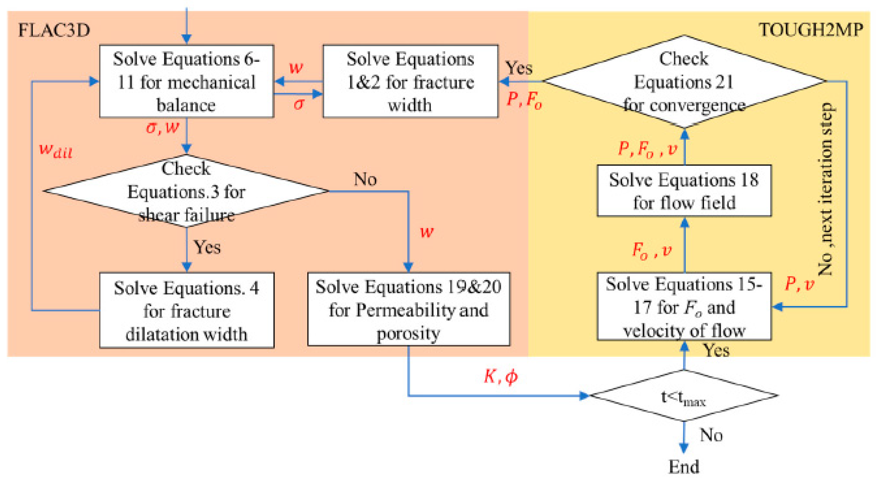
2.4. Hydro-Mechanical (HM) Coupling Framework

The coupling mode is shown in Figure 1. In each time step, TOUGH2MP collects variables from each processor and then sends them to FLAC3D for updates to permeability, porosity, and volume strain within the fractured rock. The newly obtained values of each element are transferred back to TOUGH2MP and distributed on each processor to calculate the corresponding changes in hydraulic properties. For more detailed information, refer to the literature by Liao et al. [45].

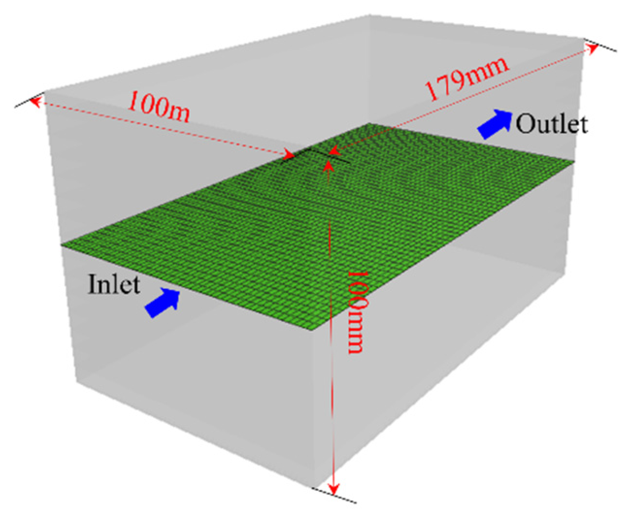
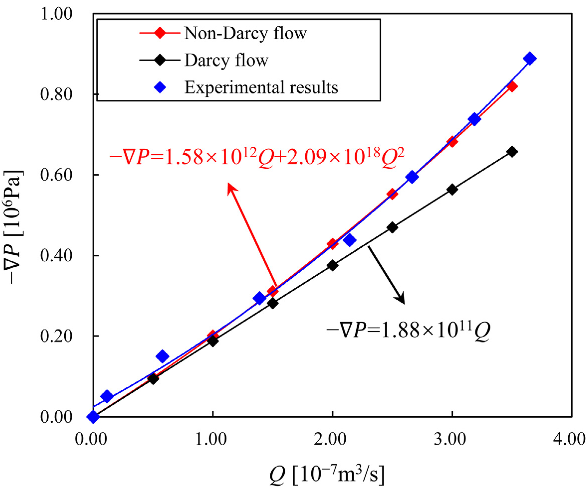
2.5. Model Validation

To validate the HM coupling model, a cubic model is generated with dimensions of 179 mm × 100 mm × 100 mm, following similar settings as in the experiments by Rong et al. [46]. As shown in Figure 2, a fracture with an initial width of 1.39 mm is embedded in the middle. A normal stress of 3.0 MPa was applied to the top side, and the normal displacement on the bottom boundary was fixed. The empirical constant q = 1.46 × 10⁻⁶ was adopted. Water was injected at the left side at a constant rate, the right side was left for free outflow, and the inlet pressure was recorded under different injection rates.

As shown in Figure 3, the pressure gradient, converted from inlet pressure, is plotted against the injection rate under different flow rates. An obvious non-linear behavior was observed on the fluid flow in the fracture, with this behavior becoming more pronounced as the flow rate increases. The linear fitting of Forchheimer’s law on the experimental results from Rong et al. and the simulated results are presented in Figure 3 as well. The simulated non-Darcy curve shows a good agreement with experimental results, confirming the feasibility of this approach in capturing the non-linear flow behavior in fractures.

To validate the plausibility of fluid velocity calculated by a simplified Equation (17), the results are compared to the results calculated by a precise Equation (22), including the injection pressure and the pressure along the fracture after 10 days. The numerical model settings and applied parameters are the same as in the experiments by Rong et al. [46], with a constant injection rate of 3.5 × 10⁻⁷ m³/s. As shown in Figure 4, the injection pressure and fracture pressure match very well in the two calculated methods, which validates the plausibility of the fluid velocity calculated the simplified Equation (17). In additional, the fracture deformation and stress state variation of this model have been previously verified, with more detailed information available in the work by Li et al. [1].

$$\stackrel{\rightharpoonup }{v}=\frac{-A+\sqrt{A^2-4B\left(\nabla p-{\rho }_w·\stackrel{\rightharpoonup }{g}\right)}}{2B}$$

(22)

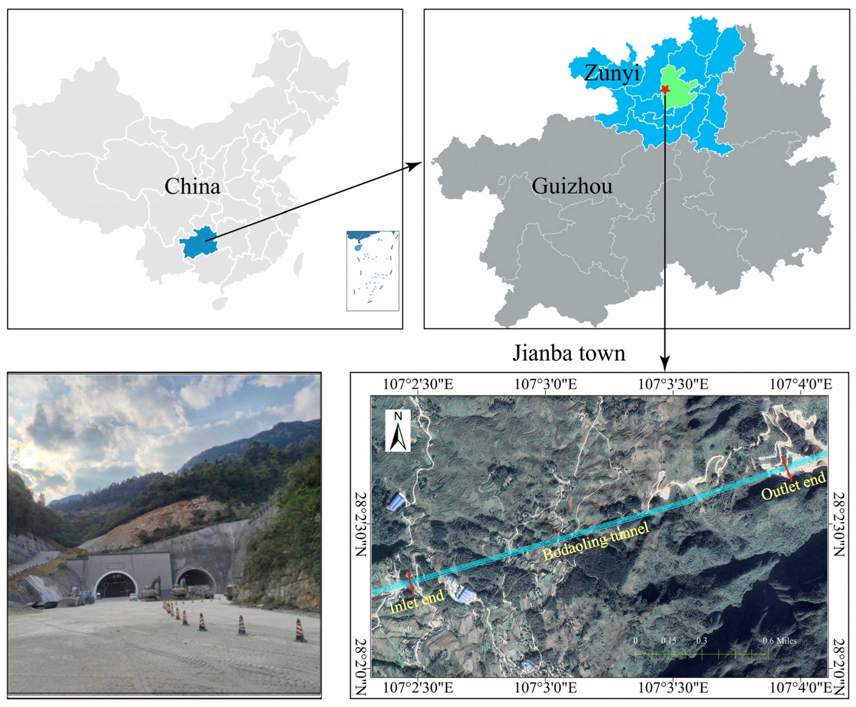
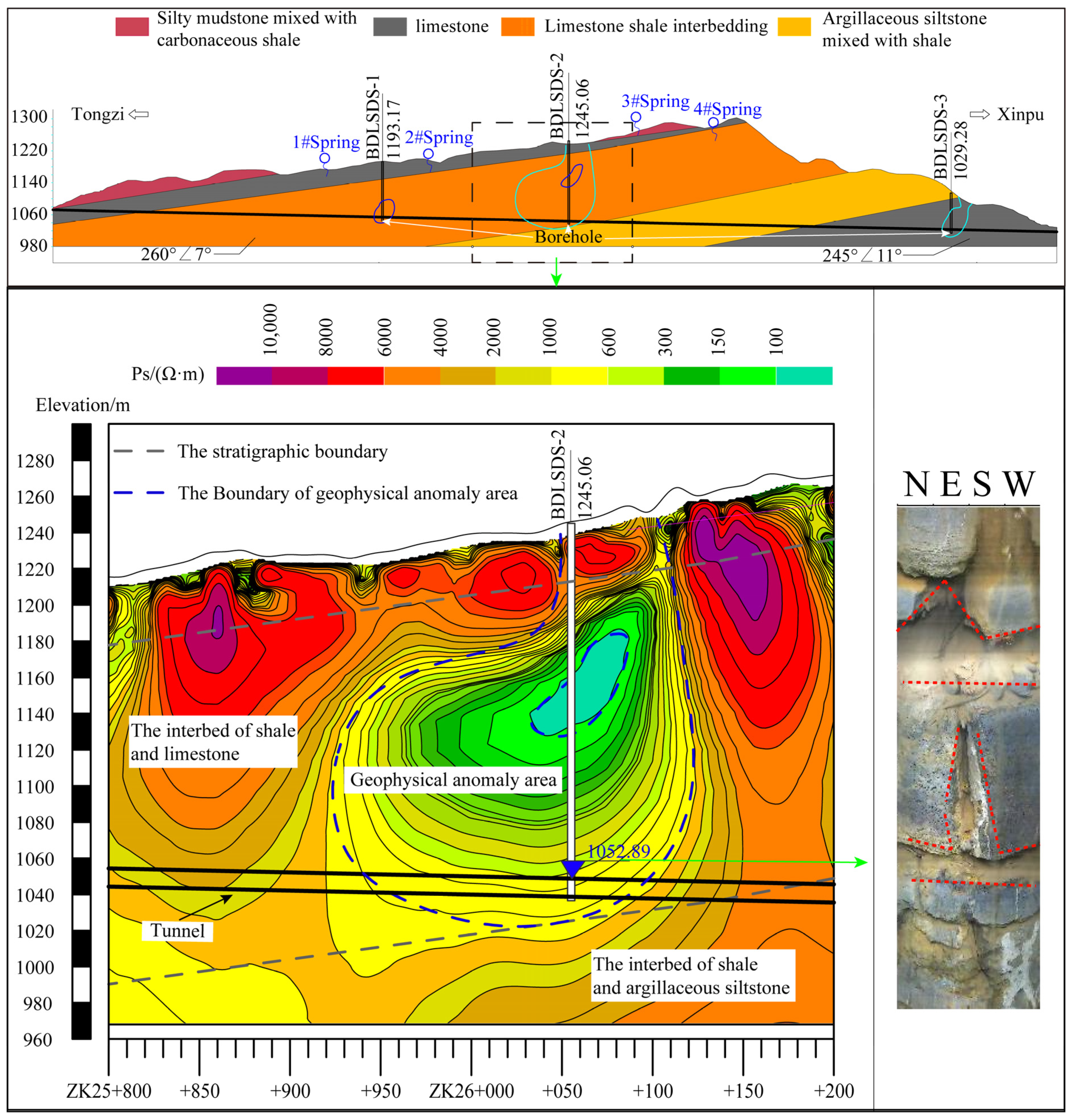
3. Engineering Geology

The project is situated in the northern Guizhou plateau region of China and characterized by an erosive karst landform. As shown in Figure 5, the entrance side features sloping terrain with a natural slope ranging from 15° to 25°. The tunnel section traverses a mountain ridge, with the highest point at an elevation of 1288.3 m. On the exit side, the terrain transitions into a river valley landscape with natural slopes ranging from 25° to 65°.

In the site area, the surrounding rock is mainly limestone shale interbedding and argillaceous siltstone mixed with shale. As shown in Figure 6, within the influence range of the tunnel route, there are four springs. These springs are the source of drinking water for local residents and have a consistent, year-round flow rate of Q = 1~10 L/s. From rock samples taken from the borehole, BDSLDS-2 reveals a relatively fractured surrounding rock mass, making water inflow likely during excavation, as shown in Figure 7. Based on field observation, the flow rate ranges from 1 to 10 L/s when there is no rainfall and can reach 100 L/s in the rainy season, posing significant challenges to the construction safety and potential danger to personnel and property. The alteration in groundwater distribution due to tunnel excavation may have an impact on the water safety of local residents. Therefore, it is essential to estimate the water inflow during tunnel excavation in order to develop appropriate countermeasures.

4. Numerical Model

The main objective of this study was to investigate water inflow in a specific tunnel section during its construction phase. In the survey report and palm face photos, it is observed that the surrounding rock in the study area exhibits a layered structure close to horizontal, with no fault passing through. The distribution of fractures shows little variation along the tunnel axis over a short distance. Therefore, we have chosen to select the tunnel section numbered ZK26 + 023 and simplify it into a two-dimensional plane, with the tunnel having a depth of 190 m, a span of 12.5 m, and a height of 10 m. To minimize the impact of boundary effects on tunnel stress, it is recommended that the model size should be at least five times larger than the tunnel size. Therefore, the horizontal dimension of the model is set to 80 m, and the vertical dimension is set to 60 m, comprising 20,042 cells and 40,646 grid points.

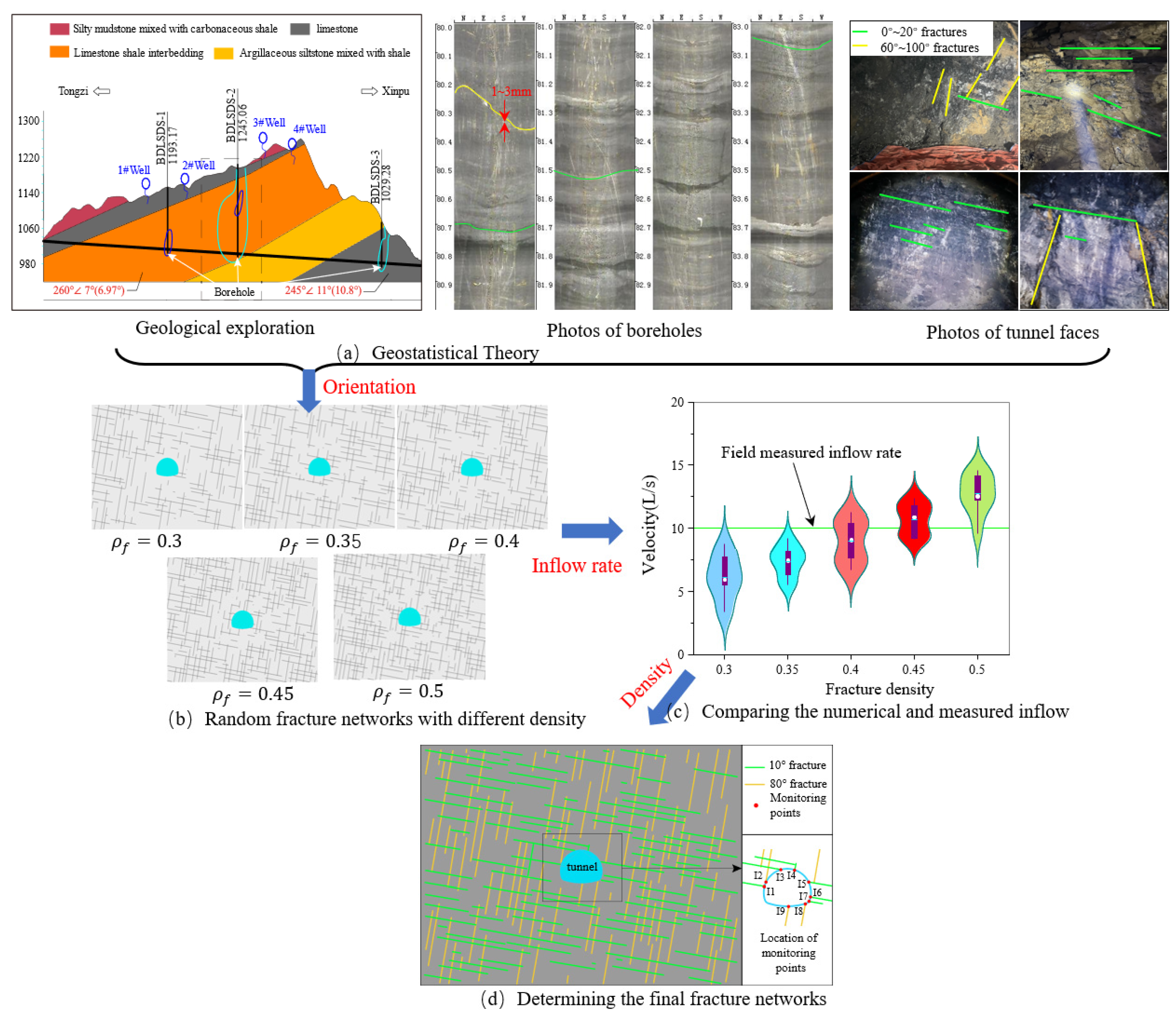
4.1. Determination of Fracture Networks

The control parameters for fracture distribution in the model include orientation, length, width, and fracture density (parameter). Since underground fractures are not fully visible, the generation of fracture networks is facilitated through geological data, numerical simulations, and field observations.

The evidence from geological exploration, borehole photos, and tunnel face images from the target site (Figure 8a) reveal abundant densely distributed natural fractures. Based on geological statistics, the natural fractures in the strata are roughly classified into two dominant clusters. One cluster’s orientation ranges from 260°∠7° to 245°∠11°, and the other cluster’s orientation is 55°∠80°. The inclination of fractures, confirmed by borehole and tunnel face photos, ranges from 60°~100° to 0°~20°, respectively. Consequently, two cluster fractures with inclinations of 10° and 80° were considered in this work. Fracture width, mainly between 0 mm and 3 mm, is also determined from borehole photos. The fracture spacing is approximately 3 m in the survey report. In geological exploration, there is no clear rule regarding the length and location of fractures. Therefore, the fracture length follows a random distribution within the range of (0, 80). Additionally, both the horizontal and vertical positions of fractures also follow random distributions within the ranges of (0, 80) and (0, 60), respectively.

The fracture density, defined as the ratio between the fracture length of the target area (Equation (23)), is a key parameter in controlling the properties of the fracture network. However, existing geological information does not fully reveal underground fracture density. To determine an appropriate fracture density, 10 random fracture networks for each fracture density were generated, totaling 50 fracture networks for five fracture densities. Samples of fracture networks for different densities are shown in Figure 8b.

$${\rho }_f=\frac{L}{A_m}$$

(23)

Here, ρ_f is the fracture density (m⁻¹), L is the total length of fractures in the model (m), and Am is the model area (m²).

As shown in Figure 8c, the simulated inflow rates on the tunnel section were compared with the field-measured value of 10 L/s. This measurement is based on the difference in temporary drain flow at the inlet and outlet of the target sections during clear or light rain conditions. It is evident that the simulated inflow rates fall within a narrow range and increase with fracture density, suggesting a clear linear correlation between inflow rate and fracture density. By comparing the average inflow rate with the field-measured value, a fracture density of 0.45 was determined in this work. Therefore, the final fracture network is established as shown in Figure 8d.

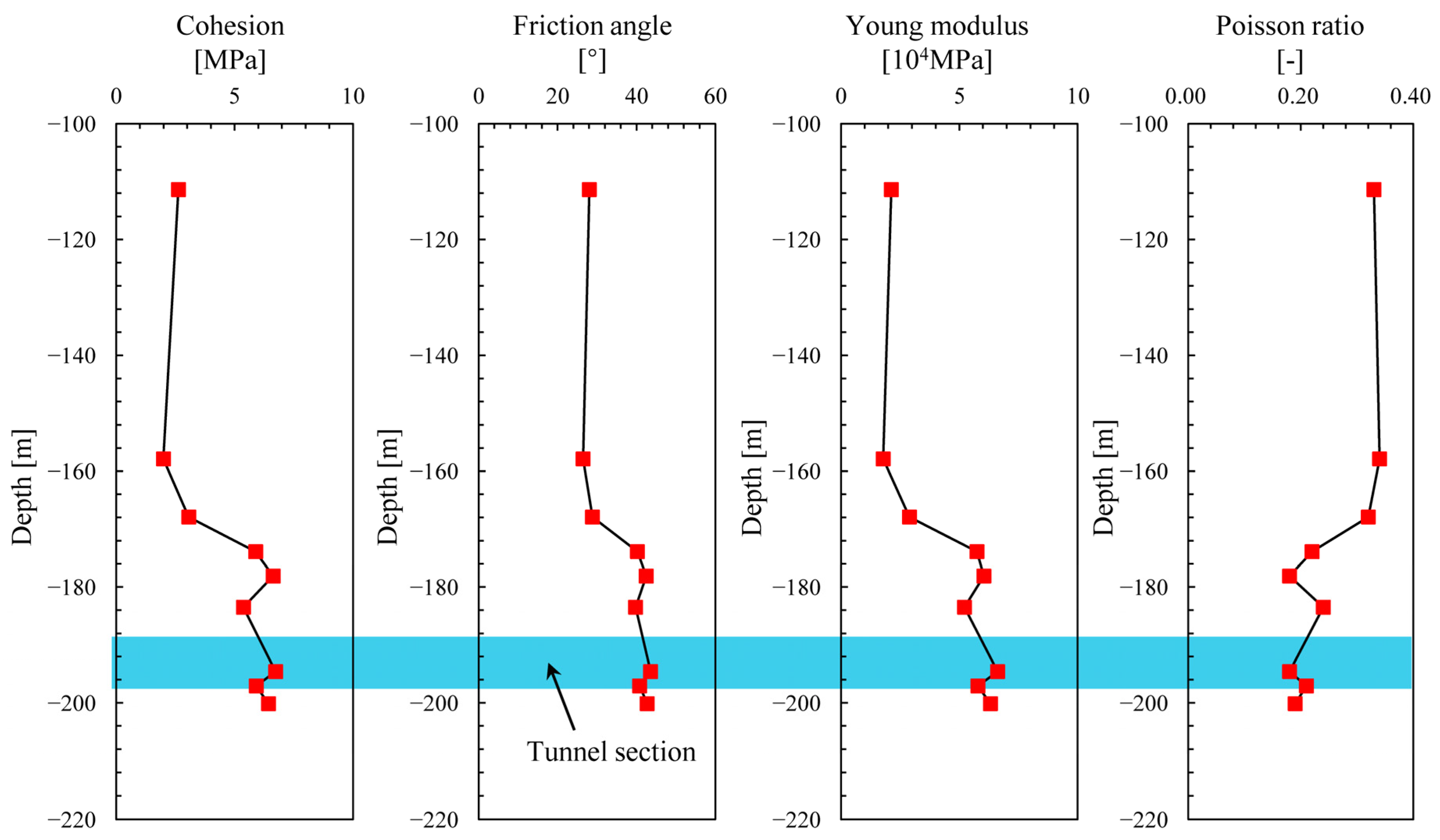
4.2. Parameter Determination

The uniaxial and direct shear tests were conducted on the intact cores from BDSDS-2 at nine different depths. The corresponding Young’s modulus, Poisson’s ratio, cohesion, and friction angle along depth are plotted in Figure 9. Young’s modulus, cohesion, and friction angle increase with depth, whereas Poisson’s ratio decreases with depth. Since the target tunnel section for water inflow is approximately 25 m away from the BDSDS-2 borehole, the corresponding mechanical properties of intact rock (Young’s modulus, Poisson’s ratio, cohesion, and friction angle) were derived from the lab result of BDSDS-2 at the depth of the tunnel section. Due to the restoration of ground stress influence on mechanical parameters and the damage to the fractured core during drilling, the mechanical properties of the fractured rock mass are referenced from literature sources. Additionally, hydraulic parameters, such as permeability and porosity, were determined based on empirical data from previous studies on limestone [12,41,47,48,49].

All calculation parameters are shown in

Table 1. Applied parameters in numerical model.

Parameter	Unit	Value	Data Source and Note
Young’s modulus E	GPa	60	Testing report of BDSDS-2
Poisson ratio v	-	0.2	Testing report of BDSDS-2
Friction angle of intact rock fI	°	44	Testing report of BDSDS-2
Cohesion of intact rock cI	kPa	6000	Testing report of BDSDS-2
Initial permeability of intact rock kI	m2	10−15	From Huang et al. [49]
Initial porosity of intact rock φI	%	2.5	From Huang et al. [49]
Friction angle of fractured rock ff	°	30	From Guo et al. [50]
Cohesion of fractured rock cf	kPa	860	From Guo et al. [50]
Initial fracture width wini	mm	1	Sensitive analysis
Tortuosity τ	-	1.91	From Ahmadi et al. [40]
Empirical constant q0	-	1.46 × 10−6	From data matching

. The fracture width varies from 1 to 3 mm, which is measured from borehole photos (see in Figure 8a). However, in deeper surrounding rock, the fracture width cannot be directly measured. Yet, the fracture width significantly influences tunnel inflow, as it serves as the primary flow channel. Consequently, the fracture width is initiated as 1 mm, and its influence is studied by sensitive analysis in the range of 1~3 mm in this work. The tortuosity τ of 1.91 is taken after Ahmadi, Abbasian Arani, and Lasseux [40]. The empirical constant q₀ = 1.46 × 10⁻⁶ is taken from data matching during model validation, and its influence is discussed by sensitive analysis within the typical range of 8.79 × 10⁻⁷ to 2.93 × 10⁻⁵, as reported in references [12,40,42].

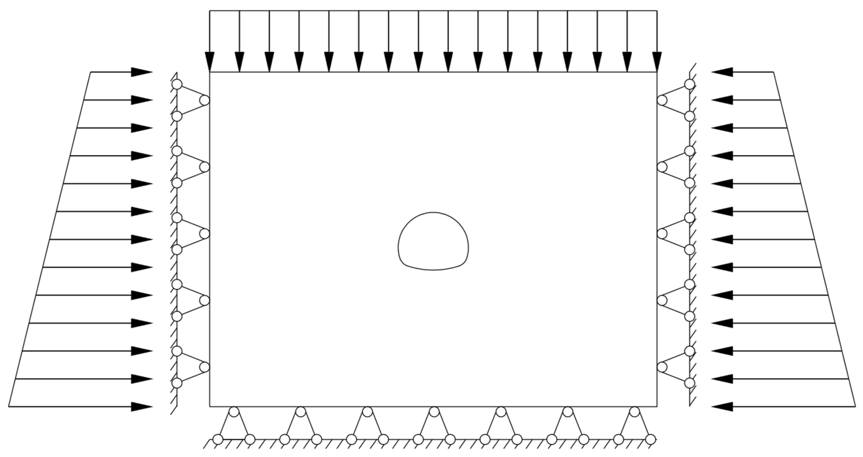
4.3. Initial and Boundary Conditions

The model’s upper boundary is situated at a depth of 190 m. The initial vertical stress is derived from a density of 2200 kg/m³, and the ratio of initial lateral pressure to initial vertical pressure is set to 0.75. As shown in Figure 10, the displacement in the normal direction at the bottom and both sides are fixed, and a constant external stress of 4.18 MPa is applied to the top boundary. The pressure on the left, right, and bottom is kept constant, and the upper boundary is designated as the free boundary and is in contact with the free water table. The horizontal plane is simultaneously positioned at the boundary of the model, precisely at an elevation of 130 m. A stable water pressure layer with a water pressure of 1.3 MPa is positioned at the top of the model. The water pressure below the top of the model is increased based on the water’s own weight base on 1.3 MPa. The total water inflow rate on the tunnel section and the individual flow rate at the intersection point (I1–I9) are recorded for evaluation of the results.

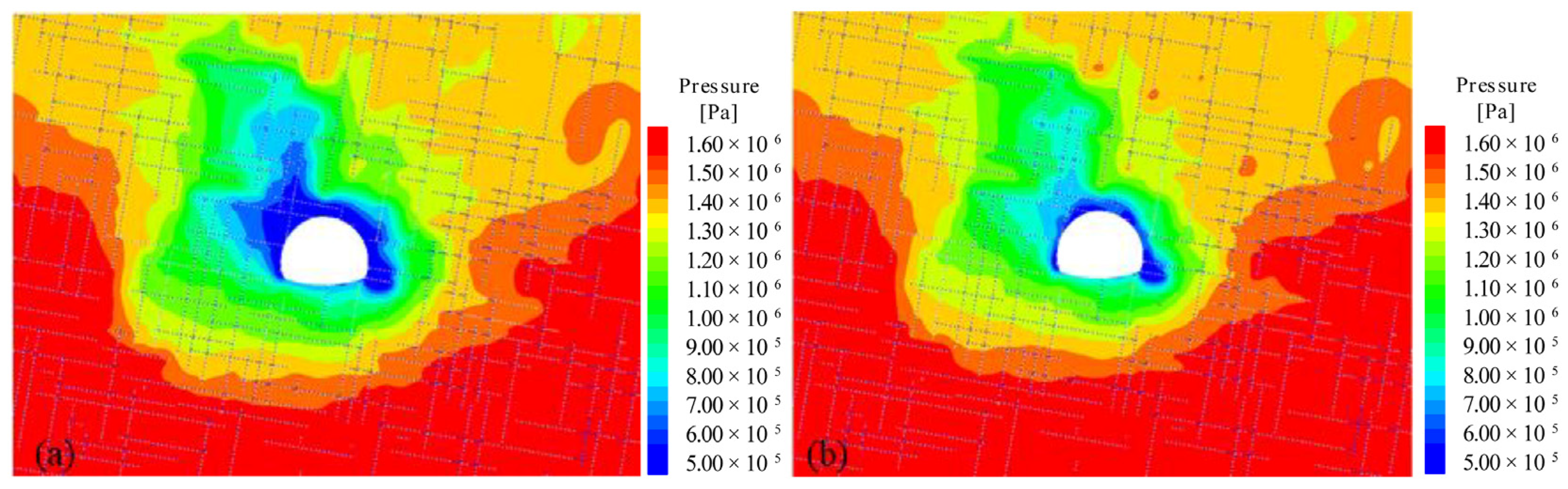
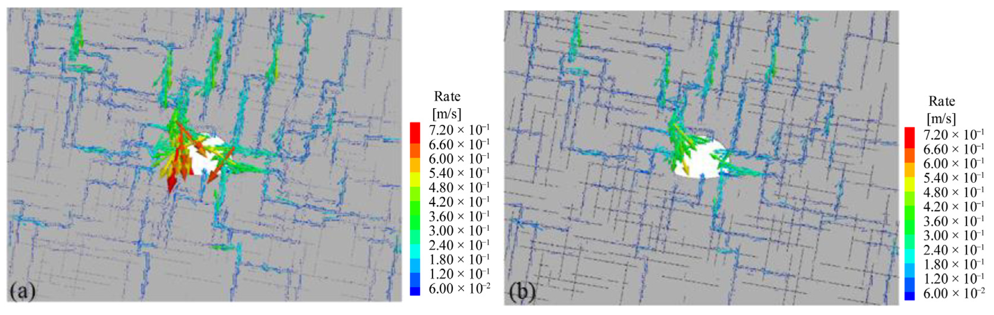
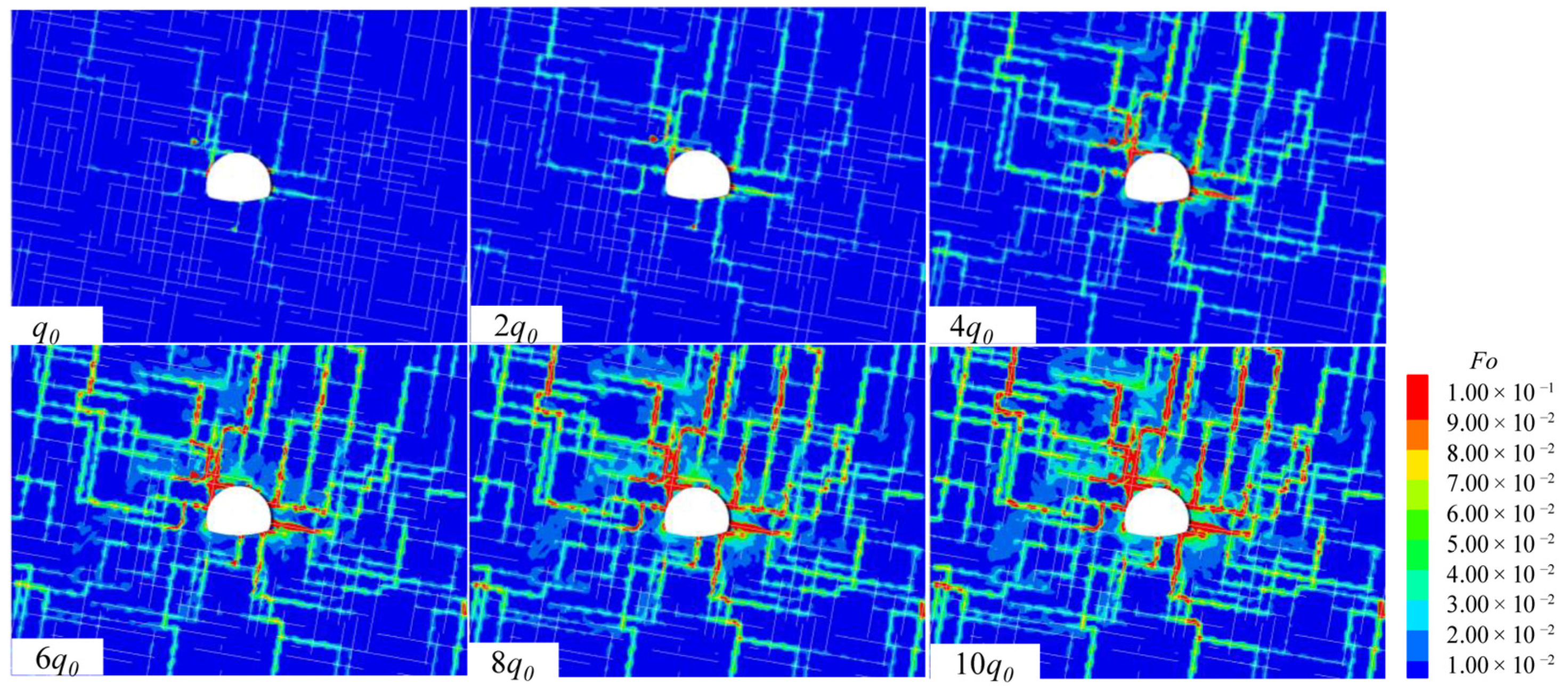
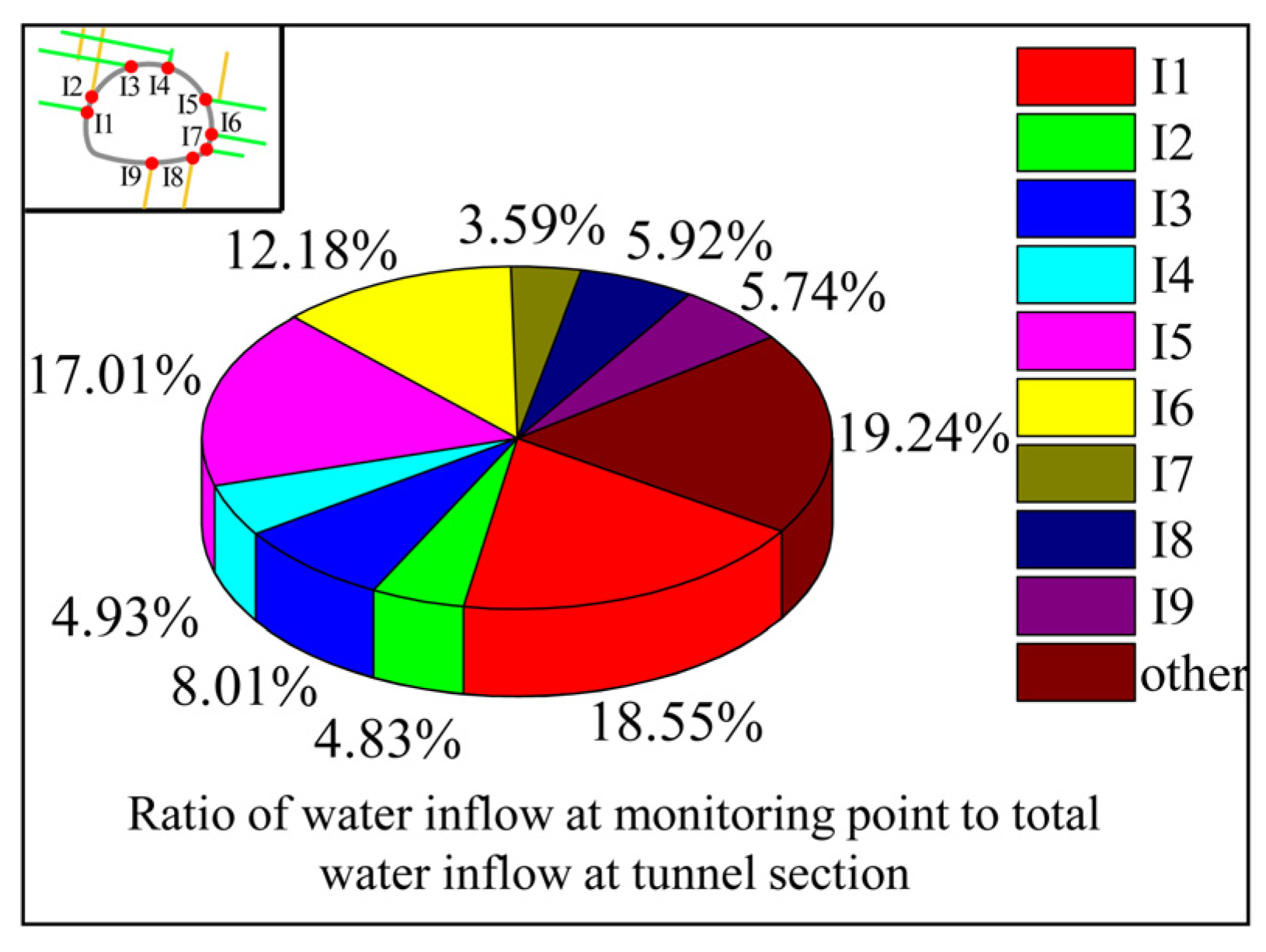
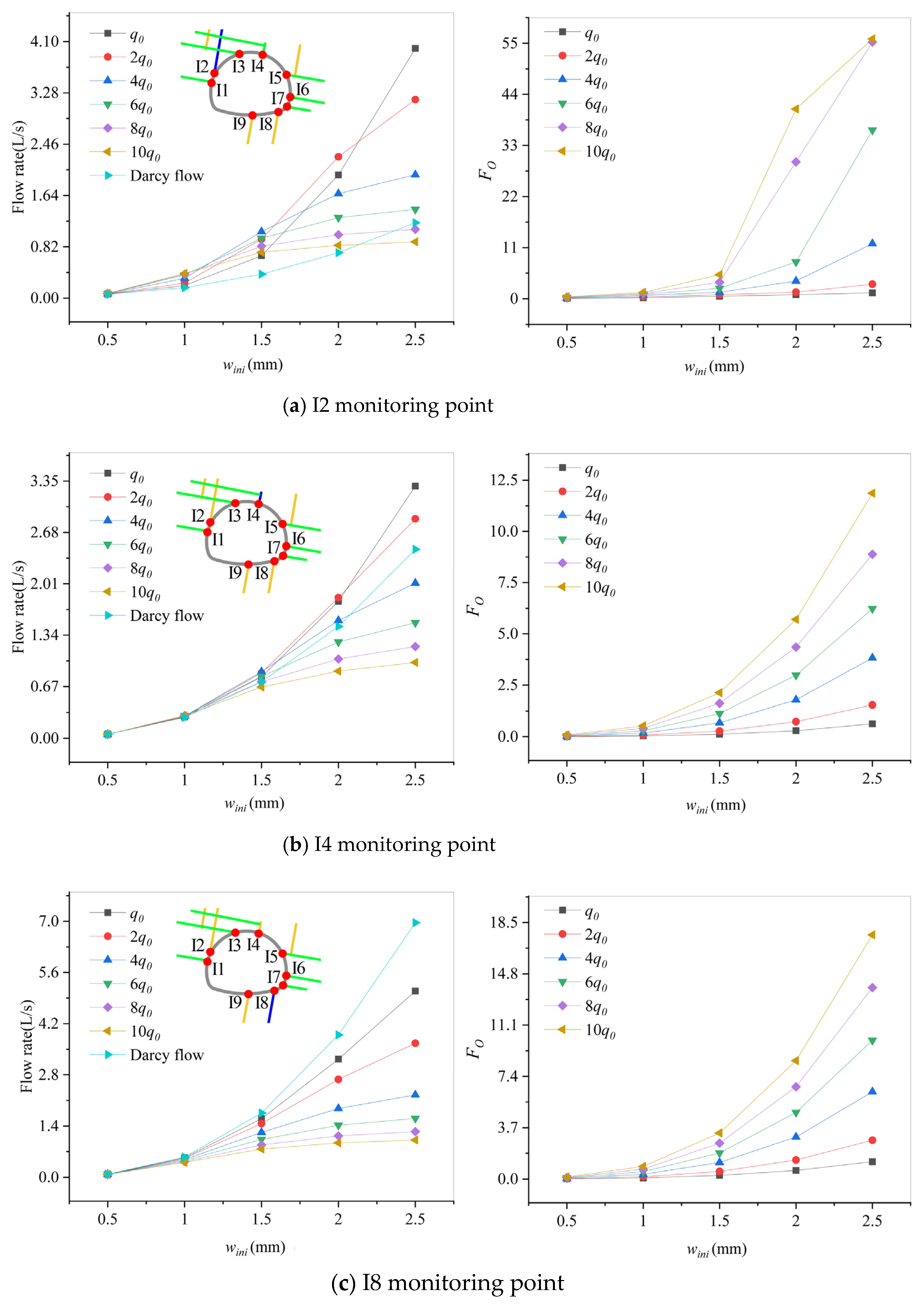
4.4. Numerical Results

The temporal total inflow rate of non-Darcy and Darcy flow along the entire tunnel section are compared in Figure 11. The inflow rate is very high during the initial stage and rapidly decreased to a stationary inflow rate within roughly 2 s. In the stationary state, the total inflow rate of Darcy flow along the entire tunnel section was 25% lower than that of non-Darcy flow, highlighting the importance of the non-Darcy effect in predicting tunnel inflow. The pressure contour of Darcy flow and non-Darcy flow in a stationary state are compared in Figure 12 and Figure 13. The low-pressure region significantly infiltrates the upper-left corner along the fractures, and the extent of infiltration in Darcy flow is much greater than that in non-Darcy flow. This is because the high flow rate is attenuated by the non-Darcy effect, which limits the extension of the low-pressure area.

The fluid velocities of Darcy flow and non-Darcy flow are shown in Figure 14a,b, respectively. As the permeability of fracture is extremely high compared to the rock matrix, evident channeling flow is observed in this fractured rock mass. Notably, the maximum flow velocity of Darcy flow was higher than that of non-Darcy flow, consistent with the inflow rate shown in Figure 11. In both cases, the maximum flow velocity was found at the intersection points of fractures and the tunnel section, which are crucial for evaluating water inflow. Therefore, the inflow rate at these intersection points in the stationary flow stage are presented in Figure 15 and

Table 2. Comparison between Darcy flow and non-Darcy flow.

Number	Velocity/(L/s)		Decrease Rate (%)	Fo
	Darcy Flow	Non-Darcy Flow
I2	0.17	0.39	−137	1.37
I4	0.27	0.29	−7	0.53
I7	0.49	0.57	−16	1.67
I3	0.53	0.66	−25	2.35
I8	0.55	0.41	26	0.91
I9	0.56	0.42	25	0.92
I6	1.19	0.87	27	5.33
I5	1.92	1.01	47	15.45
I1	3.17	0.99	69	12.87

. There was a notable difference in inflow rate between Darcy flow and non-Darcy flow when the flow rate at intersection points exceeded 0.55 L/s. Conversely, the difference in inflow rate was not sizeable between Darcy flow and non-Darcy flow. At intersection point I5, the difference reached 69%, and the F_o value reached 12.87. This phenomenon is attributed to the non-Darcy effect. Higher flow rates lead to greater resistance, resulting in large deviations of non-Darcy flow from Darcy flow, whereas lower flow rates reduce such effects. However, there is an exception at intersection point I2, where the inflow rate of Darcy flow is lower than that of non-Darcy flow, because the intersection points I1, I2, I3, and I4 are connected with each other through the fracture network. When the inflow rate at intersection point I1 is significantly limited by the non-Darcy effect, the fluid is redirected to neighboring intersection points, such as I2, I3, and I4. It is clear that non-Darcy flow substantially reduces water inflow relative to Darcy flow for flow velocities above a certain threshold. However, the variation in inflow rate at each intersection point within connected fracture networks is often uneven. In general, the inflow rate at intersection points of fractures and tunnel sections is higher than that at other locations in the tunnel section, and different intersection points react differently to the non-Darcy effect. In summary, when predicting water inflow into tunnels, it is necessary to consider the combined effect of non-Darcy flow and complex fracture networks.

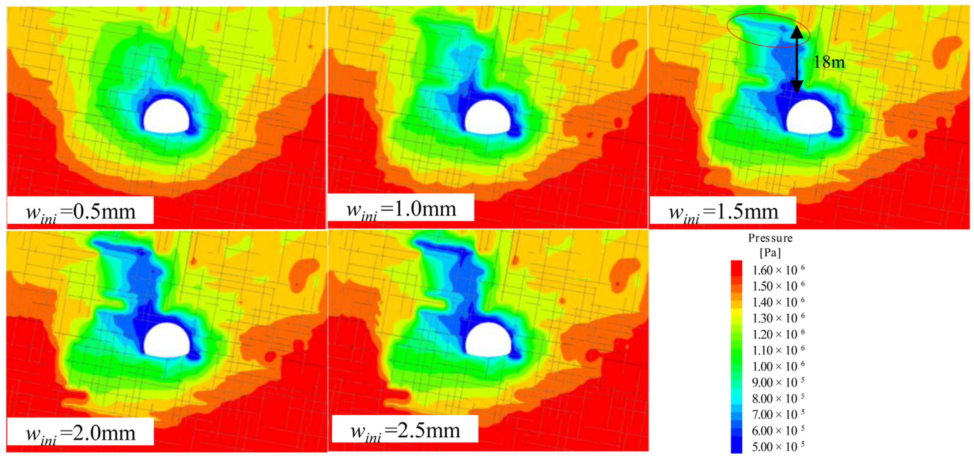
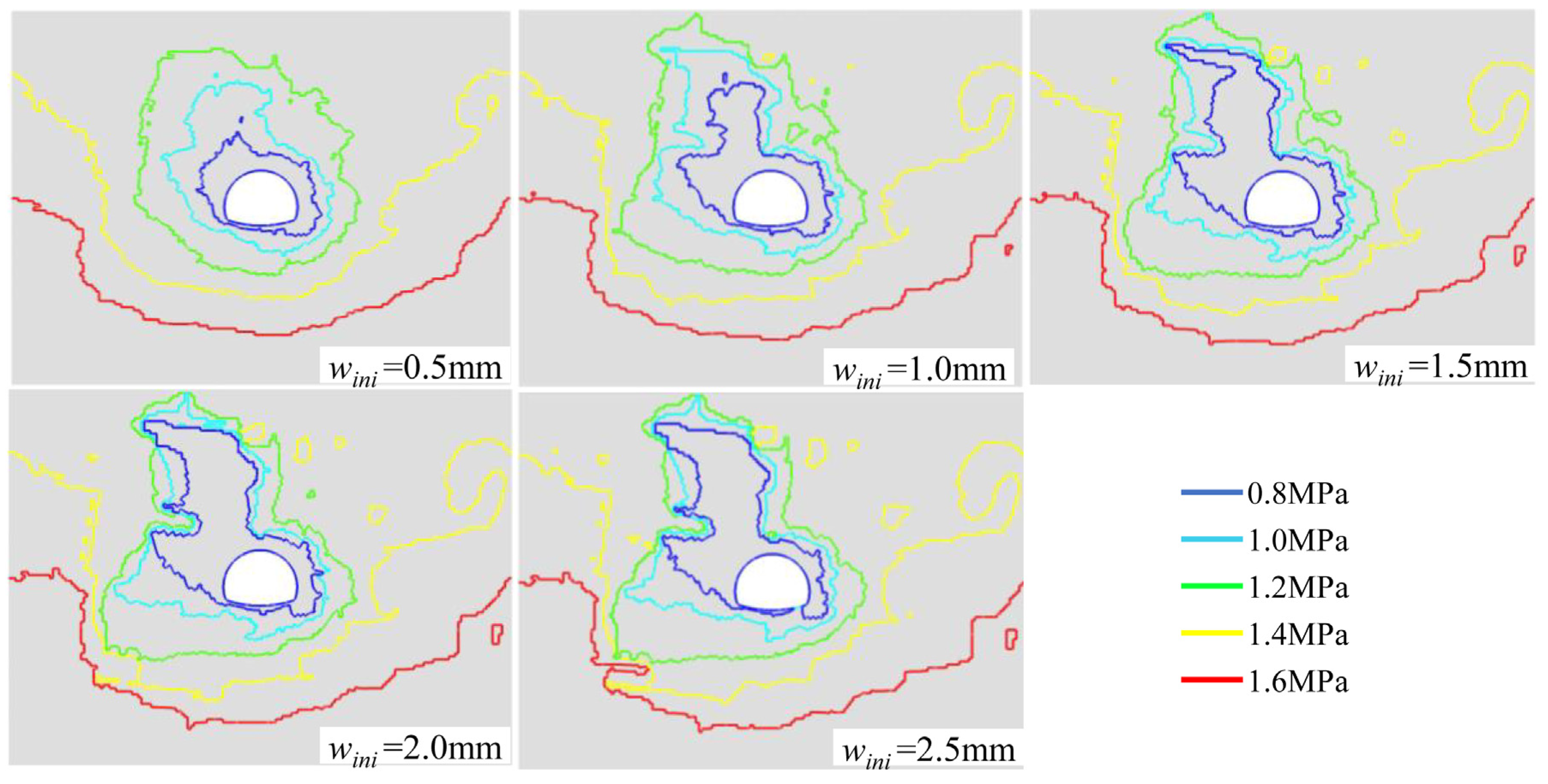
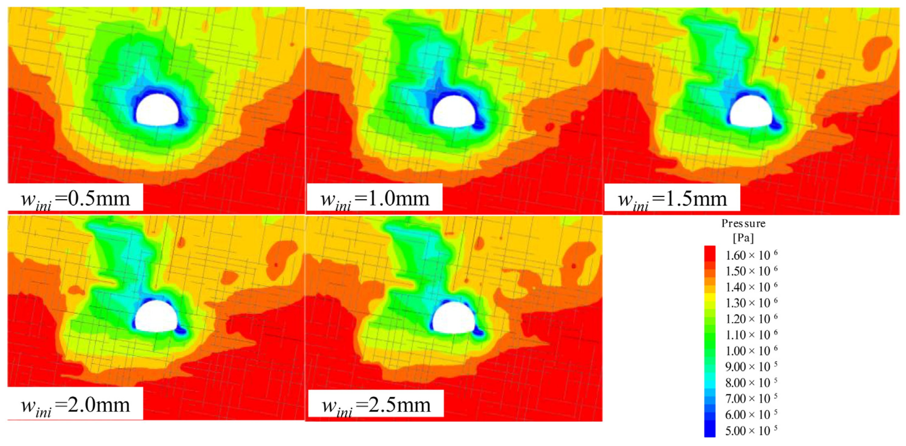
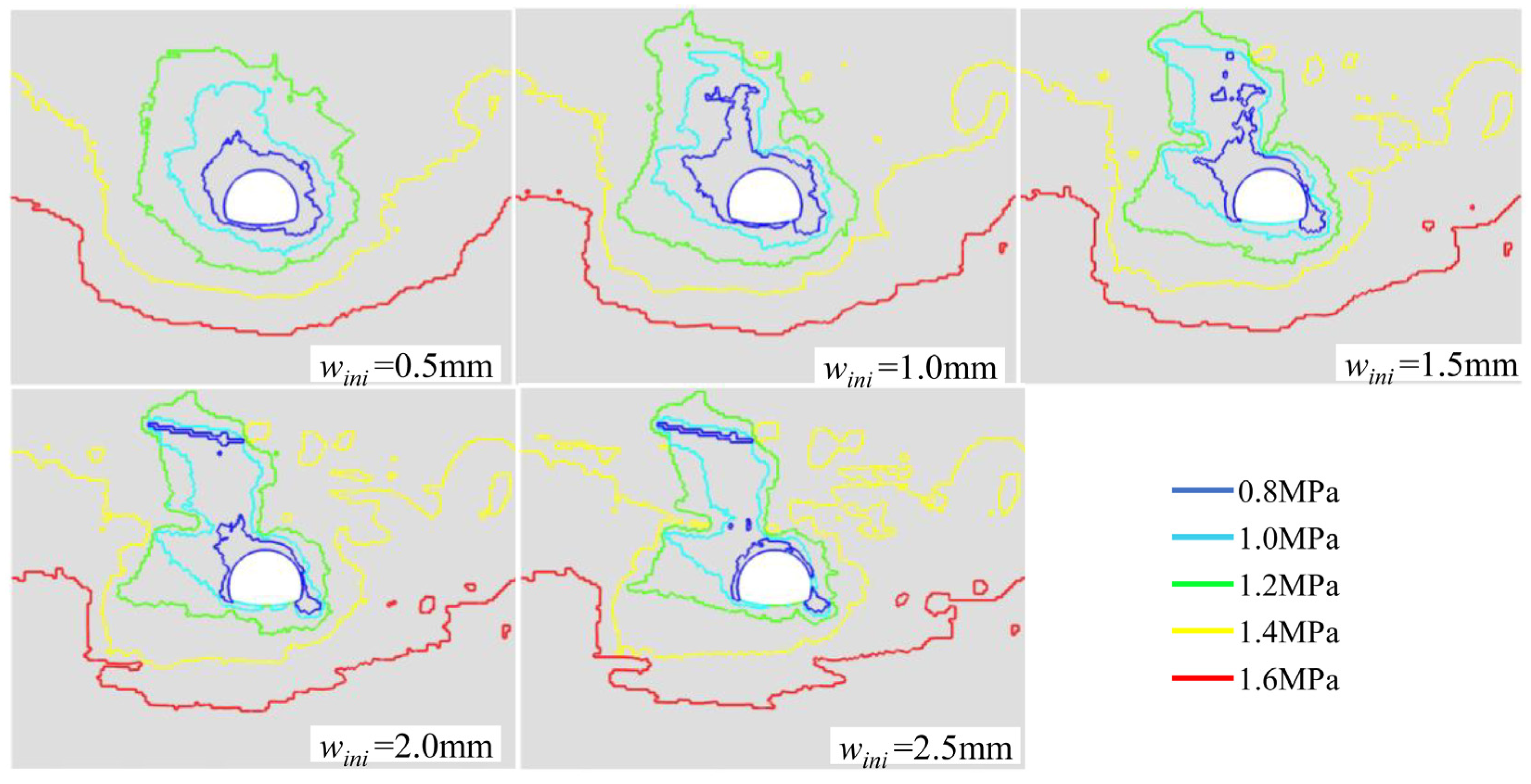
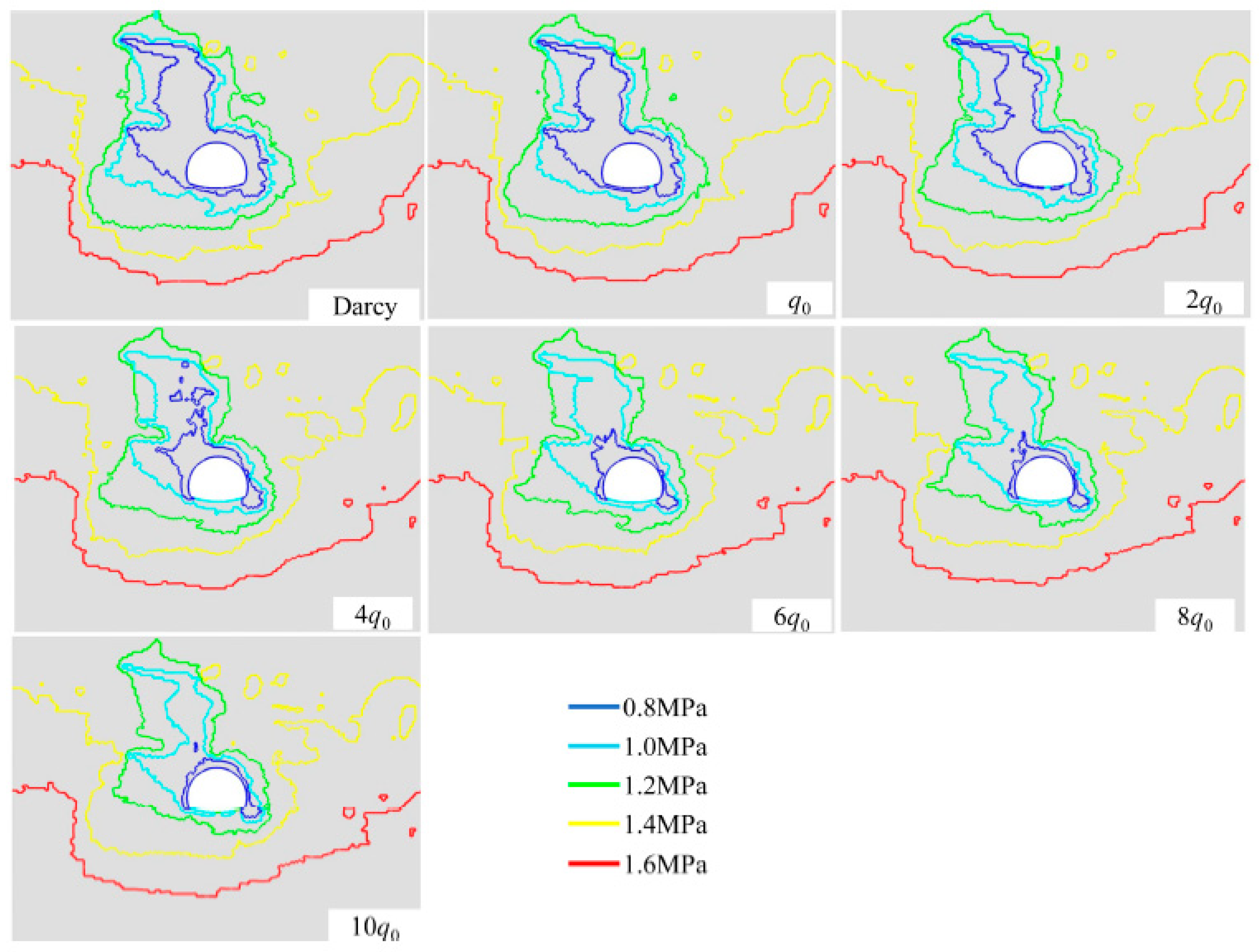
4.5. The Effect of Fracture Features and Non-Darcy Effect

This work primarily focuses on the combined effects of fracture networks and non-Darcy flow. As the fractures features and non-Darcy effect cannot be directly measured in the field, the influence of fracture features and non-Darcy flow is discussed for various initial fracture widths (w_ini) and empirical constants (q), as defined in Equation (20). In this sensitivity analysis, simulations are conducted with the initial fracture widths w_ini of 0.5 mm, 1.0 mm, 1.5 mm, 2.0 mm, and 2.5 mm and empirical constants q of q₀ (1.46 × 10⁻⁶), 2q₀, 4q₀, 6q₀, 8q₀, and 10q₀.

As shown in Figure 16a, the total water inflow rate along the entire tunnel section increases with initial fracture widths under different empirical constants q. When w_ini = 0.5 mm, the differences in water inflow rates between different q values and Darcy flow are not significant, as the non-Darcy effect is minimal with smaller fracture widths. However, the non-Darcy effect significantly increases with rising fracture widths, leading to noticeable differences between different q values and Darcy flow. Overall, the inflow rate decreases from Darcy flow to the case with higher q values. When w_ini = 2.5 mm and q = q₀, the difference between Darcy flow and non-Darcy flow is about 31%, and for q = 10q₀, it increases to 73%.

To quantify the contribution of fractures to the inflow rate, a parameter $\eta$ is defined as the ratio of inflow rate from fractures and total inflow rate along the entire tunnel section (Equation (24)). The parameter η for different initial fracture widths and empirical constants is compared in Figure 16b. Under Darcy flow conditions, the contribution of fractures on the water inflow rate increases continuously from 65% to over 90% with w_ini rising from 0.5 mm to 2.5 mm. Meanwhile, the increasing rate slows down with increasing initial fracture width. Considering the non-Darcy effect, the contribution of fractures to the water inflow rate gradually grows at lower w_ini values, since wider fractures can provide highly conductive channels for fluid. Once the initial fracture width w_ini exceeds a certain threshold, the contribution of fractures to the water inflow rate generally decreases compared to Darcy flow. This is because the non-Darcy effect occupies the dominant position for controlling fluid flow. In this case, the q values have no significant impact on the contribution of fractures on water inflow when q ≥ 4q₀ and w_ini ≥ 1.5 mm.

$$\eta =\frac{\mathrm{inflow} \mathrm{rate} \mathrm{from} \mathrm{fracture}}{\mathrm{total} \mathrm{inflow} \mathrm{rate}}$$

(24)

As discussed above, when q ≥ 4q₀ and w_ini ≥ 1.5 mm, the influence of the non-Darcy effect on water flow rates becomes significant. Therefore, in the sensitivity analysis of w_ini, we set q = 4q₀, and in the sensitivity analysis of q values, we set w_ini = 1.5 mm. The pressure contours of Darcy flow under different initial fracture widths are illustrated in Figure 17 and Figure 18. A non-symmetric drawdown of groundwater was observed from the numerical results. The height of the groundwater drawdown along the fractures on the upper-left corner of the tunnel section increases with fracture width, as a wider fracture width provides a much more conductive channel for fluid, and most of the flow concentrates in these fractures. When w_ini = 1.5 mm, a new low-pressure zone is formed at the intersection of a 10° inclined fracture and an 80° fracture, about 18 m above the tunnel arch. As w_ini further increases from 1.5 mm to 2.0 mm, this low-pressure zone continuously expands.

In Figure 19 and Figure 20, when q = 4q₀, the low-pressure zone, indicated by blue, expands as the initial fracture width w_ini increases from 0.5 mm to 1.0 mm and contracts with the decrease in initial fracture width w_ini from 1.0 mm to 2.5 mm. This contraction occurs because the significant non-Darcy effect under a high fracture width limits the propagation of the low-pressure area. Overall, the groundwater drawdown, shown in green, gradually contracts with increasing initial fractures w_ini, since the channeling flow is strengthened in the fracture network with a higher fracture width, causing the fluid flow to concentrate in certain fractures. Notably, the variation in low-pressure zones at intersections of fractures with tunnel sections is relatively small.

In Figure 21, the F_o value gradually increases within fractures with the growing initial fracture width w_ini, confirming the tendency of the non-Darcy effect shown in Figure 14a. Specifically, this variation in F_o is more significant in fractures close to the tunnel section, where the high-pressure gradient intensifies the non-Darcy effect. In addition to this, the variation in F_o in fractures with an incline angle of 80° was significant as well, wherein the fluid velocity is much higher than that in other fractures (see in Figure 12). When the value of F_o exceeds 0.11, the non-Darcy effect is significant [51,52,53,54,55]. In the case with w_ini = 1.5 mm, the F_o value reaches 0.11 at several locations along the excavation face fractures, with fracture flow dominating the water inflow rate.

The pressure contours under different q values are compared in Figure 22 and Figure 23. Interestingly, the channeling flow is alleviated with increasing q, as indicated by the gradually contracted low-pressure zone (colored blue). This is observed because the flow rate is significantly limited under higher q values. Meanwhile, the groundwater drawdown (colored green) is almost unaffected by different q values.

In Figure 24, the F_o of the whole model continues to rise with the increase in q. In this process, the growth in F_o is most pronounced at intersections of fractures and tunnel sections, followed by intersections of fractures, and then some 80° fractures. This order was consistent with the pattern observed in Figure 17. Additionally, when q ≥ 4q₀, the region around the tunnel section where F_o reaches 0.11 noticeably expands. However, for q values of 8 q₀ and 10 q₀, there was no significant change in the F_o value around the tunnel section. Therefore, it is concluded that when q is greater than or equal to 6 q₀, the influence of the q value on non-Darcy flow tends to stabilize.

The contribution of each intersection point to the total water inflow was calculated. As depicted in Figure 25, the I1, I3, and I5 points account for 43.57% of the total water inflow. Notably, these three points are associated with 10° fractures. Therefore, these three points are studied as representatives of the 10° fracture. To provide a basis for contrasting the non-Darcy flow characteristics with 80° fractures, I2, I4, and I8 were selected as reference points. Consequently, the two groups of intersection points were selected as the main research objects in the following discussion.

As shown in Figure 26a, I1 is located on the left side of the tunnel section, adjacent to I2. Its flow rate rises with increase in w_ini and a decrease in q. Furthermore, when w_ini ≥ 1.5 mm, the non-Darcy flow effect significantly influences the flow rate. If q ≥ 4q₀, the flow rates for various q values are relatively close. This pattern aligns with the observations in Figure 14 and Figure 15. Notably, the flow rate tends to 2.3 L/s, and F_o tends to 26 when w_ini = 1.5 mm and q ≥ 6q₀.

As shown in Figure 26b, I3 belongs to the fracture network connecting I2 and I4. The overall flow rate is lower than I1. When w_ini ≤ 2.0 mm and q ≤ 4q₀, the flow rate of non-Darcy flow is higher than that of Darcy flow. Additionally, when w_ini ≥ 2.0 mm and q ≥ 6q₀, the increase in flow rate and F_o is less than 0.7 L/s and less than 2, respectively. The non-Darcy flow effect tends to stabilize.

In Figure 26c, I5 intersects with a single 80° fracture. When q ≥ 4q₀ and w_ini = 1.5 mm, the flow rate tends to 2.3 L/s, and F_o tends to 25, which is similar to point I1. However, no matter how q changes, F_o always tends to 25 as w_ini increases. The flow rate and the non-Darcy flow effect of I5 are stable.

Comparing the three monitoring points associated with 10° fractures, the non-Darcy flow significantly impacts the flow rate when w_ini ≥ 1.5 mm. Furthermore, when q ≥ 6q₀ and w_ini ≥ 1.5 mm, the F_o tends to stabilize in I3 and I5. Within this stable range, the flow rate increases gradually from 1.9 to 2.3 L/s. Notably, though the maximum F_o of I1 is twice that of I5, the flow rate gap between I1 and I5 is smaller.

As shown in Figure 27a–c, the flow rate curves in I2, I4, and I8 follow a pattern similar as the total flow rate curves. F_o, however, does not exhibit a tendency to stabilize. Furthermore, I2 and I4 exhibit behavior similar to that of I3, where non-Darcy flow rates exceed Darcy flow rates. When w_ini ≥ 2 mm and q ≥ 6q₀, the value of F_o is close to that of I1, but their flow rates differ.

5. Discussion

A comprehensive comparison of the flow rate and F_o curves at various intersection points reveals that changes in w_ini and q have a significant impact on the inflow from fractures. As w_ini increases, the flow rate also increases, and the non-Darcy effect becomes stronger. This phenomenon occurs because inertial pressure drops are controlled by the flow rate [56,57,58], and the permeability increases simultaneously with the increase in fracture width. According to Equations (16) and (21), an increase in permeability leads to a higher flow rate and F_o value, which is consistent with the findings of Cao et al. [59], Xue et al. [60], and Cherubini et al. [61]. Similarly, higher q values result in a stronger non-Darcy effect and reduced flow rates, as observed in the results of Gattinoni et al. [62] and Nikakhtar and Zare [63]. This occurs because the non-Darcy coefficient β increases with the q value, directly enhancing the non-Darcy effect. In cases where flow velocity reaches a certain level with minimal interference from other fractures, the non-Darcy flow effect within fractures tends to stabilize when q ≥ 6q₀. This phenomenon is also evident in the relationship curve between the non-Darcian effect factor f and the non-Darcian coefficient β, as observed by Zhou, Liu, Li, He, Tang, and Zhao [28] and Liu, Zhou, Li, Tan, and Hou [29]. This aligns closely with the results obtained from the overall tunnel section analysis discussed earlier.

Additionally, the angle of fractures also influences the non-Darcy flow effect [64]. In the entire model, the flow rate in the 80° fracture was faster than that in the 10° fracture due to the larger water pressure gradient in the vertical direction. However, in the tunnel section, the largest water inflow occurs at I1 and I5, which contain 10° fractures. This is because the fixed hydraulic boundaries maintain a horizontal water pressure gradient on both sides. In contrast, the 80° fractures often connect to variable head boundaries above, leading to a reduction in flow velocity as water pressure changes. Unlike the general rule in other research that Darcy flow is higher than the non-Darcy flow under equal conditions, as in Lee, Lee, and Yeo [26], Geng et al. [65], and Jia et al. [66], a portion of the flow with higher velocity, such as I1, is diverted through the fracture network to regions with lower velocity (I2, I3, I4) because of the obstruction of the non-Darcy effect. As a result, non-Darcy flow exceeds the Darcy flow, highlighting the influence of complex fracture networks and the non-Darcy flow effect on water flow.

6. Conclusions

In this work, a hydro-mechanical coupling model based on a discrete fracture network was proposed to predict tunnel water inflow, considering the impact of non-Darcy flow. The model’s effectiveness was confirmed through comparison with experimental data and field measurements from the Baduoling Tunnel in Guizhou, China. The following important conclusions can be drawn:

(1)

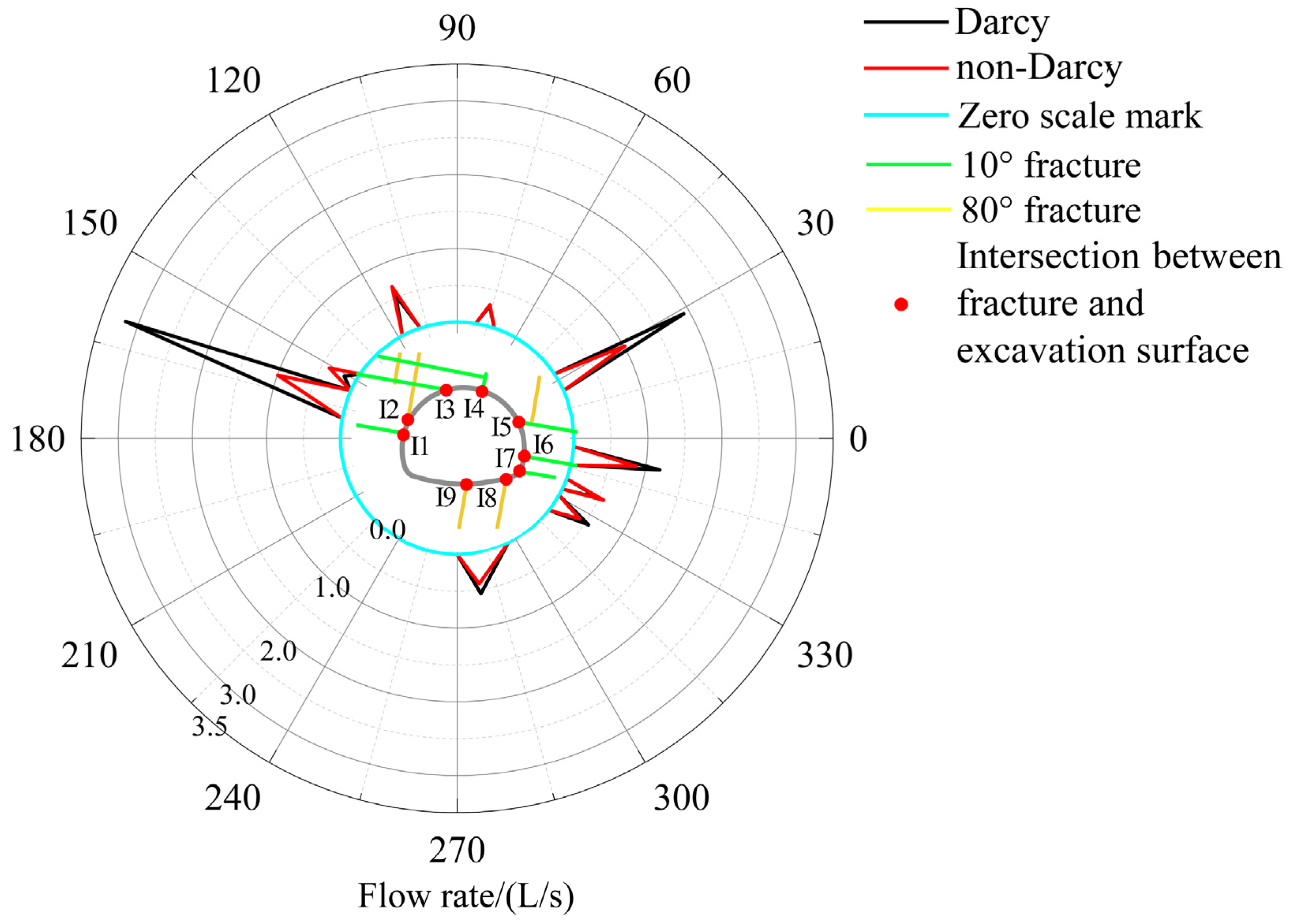
Darcy flow tends to overestimate water inflow, especially when fracture widths range from 0 to 3 mm, with Darcy flow exceeding non-Darcy flow by up to 25%, consistent with previous research by Chen, Liao, Zhou, Hu, Yang, Zhao, Wu, and Yang [12] in karst tunnels of Guizhou.

(2)

Increasing initial fracture width results in higher flow rates and stronger non-Darcy effects. Additionally, raising the q value further intensifies the non-Darcy effects and reduces flow rates. However, there is a threshold value at which the impact of non-Darcy effects slows down, and this threshold value is approximately 8.77 × 10⁻⁶ for the Bodaoling Tunnel.

(3)

The interaction of non-Darcy flow and complex fracture networks results in intricate flow patterns. Non-Darcy flow obstruction can redirect flow through the fracture network to adjacent inflow points, causing non-Darcy flow to be faster than Darcy flow at specific locations. This underscores the necessity of considering the non-Darcy effect in predicting water inflow in complex fractured rock masses.

The research primarily focuses on the fracture characteristics in two-dimensional space and the impact of non-Darcy flow on water inflow. Due to the inherent complexity of geological environments in practical engineering, such as fracture characteristics and the evolution of geological conditions in three dimensions, the accuracy of model generation methods may be limited. Additionally, during the excavation of the Badaoling Tunnel, various karst structures were observed, including fractures, caves, and underground rivers. Though these factors were not fully addressed in this study, they will be incorporated into future research to enhance the model’s engineering applicability.

References

1. Li, G.; Li, C.; Liao, J.; Wang, H. A New Hydro-Mechanical Coupling Numerical Model for Predicting Water Inflow in Karst Tunnels Considering Deformable Fracture. Sustainability 2023, 15, 14703. [Google Scholar] [CrossRef]
2. Qin, Y.; Lai, J.; Gao, G.; Yang, T.; Zan, W.; Feng, Z.; Liu, T. Failure analysis and countermeasures of a tunnel constructed in loose granular stratum by shallow tunnelling method. Eng. Fail. Anal. 2022, 141, 106667. [Google Scholar] [CrossRef]
3. Shahriar, K.; Sharifzadeh, M.; Hamidi, J.K. Geotechnical risk assessment based approach for rock TBM selection in difficult ground conditions. Tunn. Undergr. Space Technol. 2008, 23, 318–325. [Google Scholar] [CrossRef]
4. Li, L.; Lei, T.; Li, S.; Zhang, Q.; Xu, Z.; Shi, S.; Zhou, Z. Risk assessment of water inrush in karst tunnels and software development. Arab. J. Geosci. 2015, 8, 1843–1854. [Google Scholar] [CrossRef]
5. Peng, L.J. Existing Operational Railway Tunnel Water Leakage Causes and Remediation Technologies. Adv. Mater. Res. 2014, 1004–1005, 1444–1449. [Google Scholar] [CrossRef]
6. Zhang, Y.; Zhang, D.; Fang, Q.; Xiong, L.; Yu, L.; Zhou, M. Analytical solutions of non-Darcy seepage of grouted subsea tunnels. Tunn. Undergr. Space Technol. 2020, 96, 103182. [Google Scholar] [CrossRef]
7. Wu, Q.; Wang, M.; Wu, X. Investigations of groundwater bursting into coal mine seam floors from fault zones. Int. J. Rock Mech. Min. Sci. 2004, 41, 557–571. [Google Scholar] [CrossRef]
8. Jeannin, P.-Y.; Malard, A.; Rickerl, D.; Weber, E. Assessing karst-hydraulic hazards in tunneling—The Brunnmühle spring system—Bernese Jura, Switzerland. Environ. Earth Sci. 2015, 74, 7655–7670. [Google Scholar] [CrossRef]
9. Apaydin, A.; Korkmaz, N.; Ciftci, D. Water inflow into tunnels: Assessment of the Gerede water transmission tunnel (Turkey) with complex hydrogeology. Q. J. Eng. Geol. Hydrogeol. 2018, 52, 346–359. [Google Scholar] [CrossRef]
10. Li, S.-C.; Zhou, Z.-Q.; Li, L.-P.; Xu, Z.-H.; Zhang, Q.-Q.; Shi, S.-S. Risk assessment of water inrush in karst tunnels based on attribute synthetic evaluation system. Tunn. Undergr. Space Technol. 2013, 38, 50–58. [Google Scholar] [CrossRef]
11. Chen, T.; Yin, H.; Zhai, Y.; Xu, L.; Zhao, C.; Zhang, L. Numerical Simulation of Mine Water Inflow with an Embedded Discrete Fracture Model: Application to the 16112 Working Face in the Binhu Coal Mine, China. Mine Water Environ. 2022, 41, 156–167. [Google Scholar] [CrossRef]
12. Chen, Y.-F.; Liao, Z.; Zhou, J.-Q.; Hu, R.; Yang, Z.; Zhao, X.-J.; Wu, X.-L.; Yang, X.-L. Non-Darcian flow effect on discharge into a tunnel in karst aquifers. Int. J. Rock Mech. Min. Sci. 2020, 130, 104319. [Google Scholar] [CrossRef]
13. Goodman, R.E. Ground Water Inflows during Tunnels Driving; College of Engineering, University of California: Berkeley, CA, USA, 1964. [Google Scholar]
14. Moon, J.; Fernandez, G. Effect of Excavation-Induced Groundwater Level Drawdown on Tunnel Inflow in a Jointed Rock Mass. Eng. Geol. 2010, 110, 33–42. [Google Scholar] [CrossRef]
15. Kolymbas, D.; Wagner, P. Groundwater ingress to tunnels—The exact analytical solution. Tunn. Undergr. Space Technol. 2007, 22, 23–27. [Google Scholar] [CrossRef]
16. Perrochet, P. Confined Flow into a Tunnel during Progressive Drilling: An Analytical Solution. Groundwater 2005, 43, 943–946. [Google Scholar] [CrossRef]
17. Park, K.-H.; Owatsiriwong, A.; Lee, J.-G. Analytical solution for steady-state groundwater inflow into a drained circular tunnel in a semi-infinite aquifer: A revisit. Tunn. Undergr. Space Technol. 2008, 23, 206–209. [Google Scholar] [CrossRef]
18. Sato, K.; Iizawa, M. Fundamental study on unsteady flow around underground cavern in unconfined groundwater. Proc. Jpn. Soc. Civ. Eng. 1983, 1983, 213–221. [Google Scholar] [CrossRef]
19. Shi, W.; Yang, T.; Yu, S. Experimental Investigation on Non-Darcy Flow Behavior of Granular Limestone with Different Porosity. J. Hydrol. Eng. 2020, 25, 06020004. [Google Scholar] [CrossRef]
20. Hassani, A.N.; Katibeh, H.; Farhadian, H. Numerical analysis of steady-state groundwater inflow into Tabriz line 2 metro tunnel, northwestern Iran, with special consideration of model dimensions. Bull. Eng. Geol. Environ. 2016, 75, 1617–1627. [Google Scholar] [CrossRef]
21. Zhang, K.; Xue, Y.; Xu, Z.; Su, M.; Qiu, D.; Li, Z. Numerical study of water inflow into tunnels in stratified rock masses with a dual permeability model. Environ. Earth Sci. 2021, 80, 260. [Google Scholar] [CrossRef]
22. Chen, Z.; Su, Z.; Li, M.; Shen, Q.; Fan, L.; Zhang, Y. Investigation of the Tunnel Water Inflow Prediction Method Based on the MODFLOW-DRAIN Module. Water 2024, 16, 1078. [Google Scholar] [CrossRef]
23. Jin, X.; Li, Y.; Luo, Y.; Liu, H. Prediction of city tunnel water inflow and its influence on overlain lakes in karst valley. Environ. Earth Sci. 2016, 75, 1162. [Google Scholar] [CrossRef]
24. Zhang, X.; Wang, M.; Feng, D.; Wang, J. Water Inflow Amount Prediction for Karst Tunnel with Steady Seepage Conditions. Sustainability 2023, 15, 10638. [Google Scholar] [CrossRef]
25. Quinn, P.M.; Cherry, J.A.; Parker, B.L. Quantification of non-Darcian flow observed during packer testing in fractured sedimentary rock. Water Resour. Res. 2011, 47, W09533. [Google Scholar] [CrossRef]
26. Lee, S.H.; Lee, K.; Yeo, I.W. Assessment of the validity of Stokes and Reynolds equations for fluid flow through a rough-walled fracture with flow imaging. Geophys. Res. Lett. 2014, 41, 4578–4585. [Google Scholar] [CrossRef]
27. Chen, Y.-F.; Zhou, J.-Q.; Hu, S.-H.; Hu, R.; Zhou, C.-B. Evaluation of Forchheimer equation coefficients for non-Darcy flow in deformable rough-walled fractures. J. Hydrol. 2015, 529, 993–1006. [Google Scholar] [CrossRef]
28. Zhou, J.-Q.; Liu, H.-B.; Li, C.; He, X.-L.; Tang, H.; Zhao, X.-J. A semi-empirical model for water inflow into a tunnel in fractured-rock aquifers considering non-Darcian flow. J. Hydrol. 2021, 597, 126149. [Google Scholar] [CrossRef]
29. Liu, H.-B.; Zhou, J.-Q.; Li, C.; Tan, J.; Hou, D. Semi-empirical models for predicting stable water inflow and influence radius of a tunnel considering non-Darcian effect. J. Hydrol. 2023, 621, 129574. [Google Scholar] [CrossRef]
30. Rui, X.; Yu, T. An efficient karst fracture seepage path construction algorithm based on a generalized disk model. Arab. J. Geosci. 2019, 12, 262. [Google Scholar] [CrossRef]
31. Zhou, J.-Q.; Gan, F.-S.; Li, C.; Tang, H. A global inertial permeability for fluid flow in rock fractures: Criterion and significance. Eng. Geol. 2023, 322, 107167. [Google Scholar] [CrossRef]
32. Huang, Z.; Zhao, K.; Li, X.; Zhong, W.; Wu, Y. Numerical characterization of groundwater flow and fracture-induced water inrush in tunnels. Tunn. Undergr. Space Technol. 2021, 116, 104119. [Google Scholar] [CrossRef]
33. Farhadian, H.; Katibeh, H.; Huggenberger, P.; Butscher, C. Optimum model extent for numerical simulation of tunnel inflow in fractured rock. Tunn. Undergr. Space Technol. 2016, 60, 21–29. [Google Scholar] [CrossRef]
34. Shi, S.; Guo, W.; Li, S.; Xie, X.; Li, X.; Zhao, R.; Xue, Y.; Lu, J. Prediction of tunnel water inflow based on stochastic deterministic three-dimensional fracture network. Tunn. Undergr. Space Technol. 2023, 135, 104997. [Google Scholar] [CrossRef]
35. Zhang, R.-H.; Zhang, L.-H.; Luo, J.-X.; Yang, Z.-D.; Xu, M.-Y. Numerical simulation of water flooding in natural fractured reservoirs based on control volume finite element method. J. Pet. Sci. Eng. 2016, 146, 1211–1225. [Google Scholar] [CrossRef]
36. Xie, Y.; Liao, J.; Zhao, P.; Xia, K.; Li, C. Effects of fracture evolution and non-Darcy flow on the thermal performance of enhanced geothermal system in 3D complex fractured rock. Int. J. Min. Sci. Technol. 2024, 34, 443–459. [Google Scholar] [CrossRef]
37. Liao, J.; Xu, B.; Mehmood, F.; Hu, K.; Wang, H.; Hou, Z.; Xie, Y. Numerical study of the long-term performance of EGS based on discrete fracture network with consideration of fracture deformation. Renew. Energy 2023, 216, 119045. [Google Scholar] [CrossRef]
38. Bandis, S.; Lumsden, A.; Barton, N. Fundamentals of rock joint deformation. Int. J. Rock Mech. Min. Sci. Geomech. Abstr. 1983, 20, 249–268. [Google Scholar] [CrossRef]
39. Itasca. Manual of FLAC3D; Itasca Consulting Group: Minneapolis, MN, USA, 2015. [Google Scholar]
40. Ahmadi, A.; Arani, A.A.A.; Lasseux, D. Numerical Simulation of Two-Phase Inertial Flow in Heterogeneous Porous Media. Transp. Porous Media 2010, 84, 177–200. [Google Scholar] [CrossRef]
41. Muljadi, B.P.; Blunt, M.J.; Raeini, A.Q.; Bijeljic, B. The impact of porous media heterogeneity on non-Darcy flow behaviour from pore-scale simulation. Adv. Water Resour. 2016, 95, 329–340. [Google Scholar] [CrossRef]
42. Ma, D.; Li, Q.; Cai, K.-C.; Zhang, J.-X.; Li, Z.-H.; Hou, W.-T.; Sun, Q.; Li, M.; Du, F. Understanding water inrush hazard of weak geological structure in deep mine engineering: A seepage-induced erosion model considering tortuosity. J. Central South Univ. 2023, 30, 517–529. [Google Scholar] [CrossRef]
43. Zhang, K.; Yamamoto, H.; Pruess, K. TMVOC-MP: A Parallel Numerical Simulator for Three-PhaseNon-Isothermal Flows of Multicomponent Hydrocarbon Mixtures Inporous/Fractured Media; Lawrence Berkeley National Laboratory Report 2007, LBNL-63827; Lawrence Berkeley National Lab. (LBNL): Berkeley, CA, USA, 2008. [Google Scholar] [CrossRef]
44. Zhou, L.; Su, X.; Lu, Y.; Ge, Z.; Zhang, Z.; Shen, Z. A New Three-Dimensional Numerical Model Based on the Equivalent Continuum Method to Simulate Hydraulic Fracture Propagation in an Underground Coal Mine. Rock Mech. Rock Eng. 2019, 52, 2871–2887. [Google Scholar] [CrossRef]
45. Liao, J.; Wang, H.; Mehmood, F.; Cheng, C.; Hou, Z. An anisotropic damage-permeability model for hydraulic fracturing in hard rock. Acta Geotech. 2023, 18, 3661–3681. [Google Scholar] [CrossRef]
46. Rong, G.; Yang, J.; Cheng, L.; Tan, J.; Peng, J.; Zhou, C. A Forchheimer equation-based flow model for fluid flow through rock fracture during shear. Rock Mech. Rock Eng. 2018, 51, 2777–2790. [Google Scholar] [CrossRef]
47. Geertsma, J. Estimating the Coefficient of Inertial Resistance in Fluid Flow Through Porous Media. Soc. Pet. Eng. J. 1974, 14, 445–450. [Google Scholar] [CrossRef]
48. de Castro, A.R.; Radilla, G. Non-Darcian flow of shear-thinning fluids through packed beads: Experiments and predictions using Forchheimer’s law and Ergun’s equation. Adv. Water Resour. 2017, 100, 35–47. [Google Scholar] [CrossRef]
49. Huang, T.; Du, P.; Peng, X.; Wang, P.; Zou, G. Pressure drop and fractal non-Darcy coefficient model for fluid flow through porous media. J. Pet. Sci. Eng. 2020, 184, 106579. [Google Scholar] [CrossRef]
50. Guo, J.; Qian, Y.; Chen, J.; Chen, F. The Minimum Safe Thickness and Catastrophe Process for Water Inrush of a Karst Tunnel Face with Multi Fractures. Processes 2019, 7, 686. [Google Scholar] [CrossRef]
51. Javadi, M.; Sharifzadeh, M.; Shahriar, K.; Mitani, Y. Critical Reynolds number for nonlinear flow through rough-walled fractures: The role of shear processes. Water Resour. Res. 2014, 50, 1789–1804. [Google Scholar] [CrossRef]
52. Zhou, J.-Q.; Hu, S.-H.; Fang, S.; Chen, Y.-F.; Zhou, C.-B. Nonlinear flow behavior at low Reynolds numbers through rough-walled fractures subjected to normal compressive loading. Int. J. Rock Mech. Min. Sci. 2015, 80, 202–218. [Google Scholar] [CrossRef]
53. Zeng, Z.; Grigg, R. A Criterion for Non-Darcy Flow in Porous Media. Transp. Porous Media 2006, 63, 57–69. [Google Scholar] [CrossRef]
54. Zhang, Z.; Nemcik, J. Fluid flow regimes and nonlinear flow characteristics in deformable rock fractures. J. Hydrol. 2013, 477, 139–151. [Google Scholar] [CrossRef]
55. Zimmerman, R.W.; Al-Yaarubi, A.; Pain, C.C.; Grattoni, C.A. Non-linear regimes of fluid flow in rock fractures. Int. J. Rock Mech. Min. Sci. 2004, 41, 163–169. [Google Scholar] [CrossRef]
56. Moutsopoulos, K.N.; Papaspyros, I.N.; Tsihrintzis, V.A. Experimental investigation of inertial flow processes in porous media. J. Hydrol. 2009, 374, 242–254. [Google Scholar] [CrossRef]
57. Tzelepis, V.; Moutsopoulos, K.N.; Papaspyros, J.N.; Tsihrintzis, V.A. Experimental investigation of flow behavior in smooth and rough artificial fractures. J. Hydrol. 2015, 521, 108–118. [Google Scholar] [CrossRef]
58. Yao, C.; Shao, Y.; Yang, J.; Huang, F.; He, C.; Jiang, Q.; Zhou, C. Effects of non-darcy flow on heat-flow coupling process in complex fractured rock masses. J. Nat. Gas Sci. Eng. 2020, 83, 103536. [Google Scholar] [CrossRef]
59. Cao, Z.-Z.; Xue, Y.-F.; Wang, H.; Chen, J.-R.; Ren, Y.-L. The non-Darcy characteristics of fault water inrush in karst tunnel based on flow state conversion theory. Therm. Sci. 2021, 25, 4415–4421. [Google Scholar] [CrossRef]
60. Xue, Y.; Teng, T.; Zhu, L.; He, M.; Ren, J.; Dong, X.; Liu, F. Evaluation of the Non-Darcy Effect of Water Inrush from Karst Collapse Columns by Means of a Nonlinear Flow Model. Water 2018, 10, 1234. [Google Scholar] [CrossRef]
61. Cherubini, C.; Giasi, C.I.; Pastore, N. Bench scale laboratory tests to analyze non-linear flow in fractured media. Hydrol. Earth Syst. Sci. 2012, 16, 2511–2522. [Google Scholar] [CrossRef]
62. Gattinoni, P.; Consonni, M.; Francani, V.; Leonelli, G.; Lorenzo, C. Tunnelling in landslide areas connected to deep seated gravitational deformations: An example in Central Alps (northern Italy). Tunn. Undergr. Space Technol. 2019, 93, 103100. [Google Scholar] [CrossRef]
63. Nikakhtar, L.; Zare, S. Evaluation of Underground Water Flow into Tabriz Metro Tunnel First Line by Hydro-Mechanical Coupling Analysis. Int. J. Geotech. Eng. 2020, 157, 1–7. [Google Scholar] [CrossRef]
64. Zhao, X.; Yang, B.; Niu, Y.; Yang, C. Seepage-Fractal Characteristics of Fractured Media Rock Materials Due to High-Velocity Non-Darcy Flow. Fractal Fract. 2022, 6, 685. [Google Scholar] [CrossRef]
65. Geng, S.; He, X.; Zhu, R.; Li, C. A new permeability model for smooth fractures filled with spherical proppants. J. Hydrol. 2023, 626, 130220. [Google Scholar] [CrossRef]
66. Jia, J.; Chen, Y.; Luo, H.; Ma, G. Seepage stability analysis of a deep-buried tunnel in fractured rocks based on a non-Darcy hydro-mechanical coupled method. Tunn. Undergr. Space Technol. 2023, 142, 105393. [Google Scholar] [CrossRef]
Figure 1. Schematic diagram of the coupling pattern.
Water 16 01885 g001
Figure 2. Demonstration of fracture model.
Water 16 01885 g002
Figure 3. Comparing the Darcy flow and non-Darcy flow results.
Water 16 01885 g003
Figure 4. Comparing the results calculated by Equations (17) and (22): (a) injection pressure, (b) pressure along the fracture after 10 days.
Water 16 01885 g004
Figure 5. Geographical situation.
Water 16 01885 g005
Figure 6. Geological settings of Bodaoling tunnel.
Water 16 01885 g006
Figure 7. Water and mud inrush scene from a disaster.
Water 16 01885 g007
Figure 8. Determining process for fracture networks: (a) inference evidence for the fracture orientation in target site; (b) randomly generated fracture network with different densities; (c) comparing the numerical results of different dense fracture networks with field-measured inflow rate; (d) determining the final fracture networks for simulation.
Water 16 01885 g008
Figure 9. The lab results of core from BDSDS-2.
Water 16 01885 g009
Figure 10. Schematic diagram of the mechanical model.
Water 16 01885 g010
Figure 11. Flow curve over time.
Water 16 01885 g011
Figure 12. Pressure contours after 1440 s: (a) Darcy flow, (b) non-Darcy flow.
Water 16 01885 g012
Figure 13. Contours maps after 1440 s: (a) Darcy flow, (b) non-Darcy flow.
Water 16 01885 g013
Figure 14. Flow vectors after 1440 s: (a) Darcy flow, (b) non-Darcy flow.
Water 16 01885 g014
Figure 15. Comparison of flow rates between Darcy flow and non-Darcy flow.
Water 16 01885 g015
Figure 16. (a) Flow rate curves with different wini values. (b) Water inflow from fracture ratio curve.
Water 16 01885 g016
Figure 17. Comparison of pressure contours for different wini (q = 0, time = 1440 s).
Water 16 01885 g017
Figure 18. Comparison of contour maps for different wini (q = 0, time = 1440 s).
Water 16 01885 g018
Figure 19. Comparison of pressure contours for different wini (q = 4q0, time = 1440 s).
Water 16 01885 g019
Figure 20. Comparison of contour maps for different wini (q = 4q0, time = 1440 s).
Water 16 01885 g020
Figure 21. Comparison of Fo contours for different wini (q = 4q0, time = 1440 s).
Water 16 01885 g021
Figure 22. Comparison of pressure contours for different q values (wini = 1.5 mm, time = 1440 s).
Water 16 01885 g022
Figure 23. Comparison of contour maps for different q values (wini = 1.5 mm, time = 1440 s).
Water 16 01885 g023
Figure 24. Comparison of Fo for different q values (wini = 1.5 mm, time = 1440 s).
Water 16 01885 g024
Figure 25. Percentage of water inflow distribution.
Water 16 01885 g025
Figure 26. Rate curve and the Forchheimer number curve for different initial fracture widths at 10° fracture monitoring points (time = 1440 s).
Water 16 01885 g026
Figure 27. Rate curve and the Forchheimer number curve for different initial fracture widths at 80° fracture monitoring points (time = 1440 s).
Water 16 01885 g027