Assessment of Soil Wind Erosion and Population Exposure Risk in Central Asia’s Terminal Lake Basins

Abstract

In the face of climate change and human activities, Central Asia’s (CA) terminal lake basins (TLBs) are shrinking, leading to deteriorating natural environments and serious soil wind erosion (SWE), which threatens regional socio-economic development, human health, and safety. Limited research on SWE and population exposure risk (PER) in these areas prompted this study, which applied the RWEQ and a PER model to assess the spatiotemporal changes in SWE and PER in TLBs in CA, including the Ili River Basin (IRB), Tarim River Basin (TRB), Syr Darya River Basin (SRB), and Amu Darya River Basin (ARB), from 2000 to 2020. We analyzed the driving factors of SWE and used the Hybrid Single-Particle Lagrangian Integrated Trajectory (HYSPLIT) model to simulate dust event trajectories. The findings from 2000 to 2020 show a spatial reduction trend in SWE and PER, with primary SWE areas in the Taklamakan Desert, Aral Sea Basin, and Lake Balkhash. Significant PER was observed along the Tarim River, near Lake Balkhash, and in the middle and lower reaches of the ARB and SRB. Over the past 21 years, temporal trends in SWE have occurred across basins, decreasing in the IRB, but increasing in the TRB, SRB, and ARB. Dust movement trajectories indicate that dust from the lower reaches of the SRB and ARB could affect Europe, while dust from the TRB could impact northern China and Japan. Correlations between SWE, NDVI, temperature, and precipitation revealed a negative correlation between precipitation and NDVI, suggesting an inhibitory impact of precipitation and vegetation cover on SWE. SWE also varied significantly under different LUCCs, with increases in cropland, forestland, and desert land, and decreases in grassland and wetland. These insights are vital for understanding SWE and PER in TLBs and offer theoretical support for emergency mitigation in arid regions.

1. Introduction

Soil wind erosion (SWE) is the process of detachment and displacement of surface soil particles by wind [1]. SWE is a worldwide environmental problem that affects land degradation and air quality [2], which reduces agricultural productivity, jeopardizes human health and, more seriously, leads to land desertification [3]. The SWE migration process leads to the loss of the most fertile topsoil layer [4], thus increasing land degradation [5,6]. Land degradation due to SWE accounts for about 28% of global land degradation [7]. A study indicated that land degradation, including SWE, resulted in a 4.8-fold reduction in net profits during the agricultural growing season in Central Asia (CA) [8]. In addition, SWE produces dusty weather [9], which leads to human respiratory and infectious diseases [10]. Specifically, PM2.5 particles produced by sand and dust can penetrate human bronchial tubes and cause lung cancer [11]. Therefore, the implementation of effective SWE prevention is crucial for ecological environment improvement, sustainable regional economic development, and human health and safety.

SWE has been assessed using various methods, such as direct field measurements of SWE [12], wind tunnel experiments [13], and isotope tracing techniques [14]. However, the applications of SWE monitoring equipment or wind tunnel simulation experiments have certain limitations, which can be challenging to quantitatively evaluate SWE at larger scales [15]. The aforementioned methods are unsuitable for conducting extensive quantitative spatial analyses. Owing to the continuous development and advancement of remote sensing technology, researchers have designed various SWE models, including the Wind Erosion Equation (WEQ) [16], the Revised Wind Erosion Equation (RWEQ) [17], the Wind Erosion Prediction System (WEPS) [18], the Texas Erosion Analysis Model (TEAM) [19], and the Wind Erosion Stochastic Simulator (WESS) [20]. The RWEQ model is one of the most commonly used methods among the abovementioned models. It is characterized by high computational efficiency, a large spatial and temporal span, easy access to data, simple model operation, etc., and has been widely used in the study of SWE in arid zones [3,21]. Additionally, a meta-analysis on global soil erosion conducted by Ma et al. [22] revealed that the RWEQ exhibited higher evaluation accuracy than other common wind erosion models.

CA, at the heart of the Eurasian continent, is one of the global arid regions [23]. Terminal lake basins (TLBs), also known as endorheic lakes, represent a significant category of lakes in this region [24,25]. These lakes constitute a vital component of the natural system in arid regions and are highly sensitive to both natural changes and human activities [26,27]. However, owing to the rapid expansion of oasis agriculture and the effects of climate change, TLBs in this area are experiencing severe shrinkage, contributing to a continuous deterioration of the surrounding ecological environment [26,28,29]. It is noteworthy that the shrinkage of TLBs can lead to large expanses of the lakebed drying up and the surface being exposed, making them susceptible to SWE and resulting in the formation of dust storms [30]. The Aral Sea in CA is a prime example. The gradual shrinkage of the Aral Sea has led to the formation of a new desert on the exposed lake bed, the Aral Sea Desert, which is subjected to frequent SWE, and has become a major source area of sand and dust in CA [31,32]. Reports have indicated that this disaster in the Aral Sea region has severely impacted human health in the area [33]. The occurrence of dust storms not only presents significant health risks to local residents and areas through which they pass, but also poses substantial environmental hazards downwind [34]. Population exposure risk (PER) refers to the potential adverse impacts or harm that individuals or groups may experience in their environments [35]. The PER model is used to assess the degree of risk to which a population is exposed to adverse environmental conditions [36], and the model is widely applicable and easy to operate, making it extensively used for evaluating various types of pollution and natural disasters [37,38]. The TLBs in CA are facing severe SWE problems. Formulating reasonable sand control measures is of significant importance for improving the ecological environment, agricultural productivity, and human health in this area. However, previous studies have mainly focused on the characterization of temporal and spatial changes in SWE and the analysis of drivers. The impact of human activities on SWE has been mainly explored, while the impact of SWE on humans has been neglected.

In view of this, a quantitative assessment of SWE and PER was conducted using the RWEQ model and a PER model in the TLBs in CA. Additionally, the Hybrid Single-Particle Lagrangian Integrated Trajectory (HYSPLIT) model was utilized in this study to simulate the trajectories of dust movement within the region. The objectives of this study were: (1) to quantitatively analyze the spatiotemporal changes in SWE in the TLBs in CA, (2) to examine the changes in the PER’s spatial pattern in regard to SWE in these basins, and (3) to investigate the primary factors driving SWE in these regions. The results from this study can address the lack of research related to the PER of SWE, and provide theoretical support for reducing the risk of a sudden SWE disaster in the arid lands of CA.

2. Materials and Methods

2.1. Study Area

CA is part of the arid regions in the world, covering 50 E to 95 E longitude and 35° N to 55° N latitude [39]. The topography of CA is characterized by mountains and basins, with a gradient of distribution that escalates in the east and tapers off in the west (Figure 1). CA is classified as a temperate continental climate [40]. There is considerable variation in the annual average precipitation levels across diverse regions, with typical annual rainfall ranging between 200 and 300 mm [41]. In desert regions, the annual precipitation is typically lower than 100 mm [42], whereas in mountainous areas, it can reach 1000 mm [43]. The vegetation in CA is predominantly composed of forestlands, grasslands, and croplands. Grasslands are the most extensive and cover a relatively large area, accounting for approximately 50% of CA’s overall area [44].

The TLBs in CA comprise four major river basins: the IRB, TRB, SRB, and ARB. Notably, Lake Balkhash and Lake Taitima are the TLB for the Ili and Tarim rivers, respectively [45,46], whereas the Aral Sea serves as the common TLB for both the Syr Darya and Amu Darya rivers [47]. These basins are mainly developed for irrigated agriculture [48,49,50,51], which is an important economic pillar of the CA region [52]. Climate change and increased water use for agricultural irrigation in CA have led to a steady reduction in the size of the terminal lakes in these basins [53], and exposed lake beds are vulnerable to the threat of SWE [54].

2.2. Data Resources

2.2.1. Meteorological Data

In this study, the meteorological data used to quantify the wind erosion modulus (WEM) based on the RWEQ model include temperature, precipitation, wind speed, and snowfall flux data from the ERA5-Land reanalysis dataset provided by the European Centre for Medium-Range Weather Forecasts (ECMWF), which have a finer spatial–temporal resolution and, therefore, perform well in CA and have also been widely used in global climate change studies [55,56]. In addition, Global Data Assimilation System (GDAS) meteorological data were utilized, which were used to simulate the dust movement trajectories of typical dust events in the study area based on the HYSPLIT model. These data were provided by the Air Resources Laboratory (ARL) of the National Oceanic and Atmospheric Administration (NOAA) of the United States. The specific data formats were used to drive the dust module of the HYSPLIT model [57,58].

2.2.2. Population Grid Data

The population grid data used in this study to calculate the PER, namely LandScan data, were sourced from the U.S. Department of Energy’s Oak Ridge National Laboratory (ORNL). These data are highly accurate and emphasize dynamic changes in population distribution [59,60]. Additionally, these data are widely used in studies related to PER [37,61,62].

2.2.3. Vegetation Data

The Normalized Difference Vegetation Index (NDVI) data utilized in this study were derived from the MOD13A2 V6 product, which can mitigate the impact of clouds and aerosols [63]. This dataset has been extensively utilized in studies investigating vegetation dynamics in arid regions [64,65].

2.2.4. Soil Data

The soil data provided for the RWEQ model included soil content types such as clay, silt, sand, gravel, organic matter, and calcium carbonate, and came from the Harmonized World Soil Database (HWSD). This database is jointly provided by the Food and Agriculture Organization (FAO) of the United Nations and the International Institute for Applied Systems Analysis (IIASA) in Vienna.

2.2.5. Land-Use and Land-Cover (LULC) Data

The LULC data employed in this study were obtained from the European Space Agency (ESA). This dataset consists of 6 primary classifications and 22 secondary classifications. Using this classification system, the LULC data within the study region were divided into categories such as forestland, wetland, desert land, construction land, cropland, grassland, and others.

2.2.6. Other Data

The Digital Elevation Model (DEM) data used in this study were obtained from the Central Asia Ecology and Environment Data Center. These data were used for the terrain visualization of the study area and for the calculation of the soil roughness factor in the RWEQ model. The PM2.5 data were integrated from the AOD retrieval data from MODIS, the Multi-angle Imaging SpectroRadiometer (MISR), and the Sea-viewing Wide Field-of-view Sensor (SeaWiFS).

Finally, all of the above data include the TLBs in CA and are counted as annual data using the maximum synthesis method [66], covering the period from 2000 to 2020, with a spatial resolution uniformly resampled to 1 km using bilinear interpolation [67]. The specific parameters of the data used in this study include spatial and temporal resolution, period, and links (

Table 1. Data used in this study.

Name	Resolution	Period	Link
Wind speed	Daily, 0.1° × 0.1°	1982–2020	(https://www.ecmwf.int/en/forecasts/dataset/ecmwf-reanalysis-v5 (accessed on 14 April 2023))
Temperature
Precipitation
Snowfall flux
GDAS	6 h, 0.1° × 0.1°	2006–2020	(https://psl.noaa.gov/data (accessed on 29 April 2023))
Population grid	Annual, 1 km	2000–2020	(https://landscan.ornl.gov (accessed on 15 May 2023))
NDVI	16 d, 1 km	2000–2020	(http://ltdr.nascom.nasa.gov (accessed on 19 April 2023))
Soil	N, 1 km	2013	(http://www.fao.org/soils-portal/en/ (accessed on 19 May 2023))
LULC	Annual, 300 m	1992–2020	(https://www.esa-landcover-cci.org/ (accessed on 27 May 2023))
PM2.5	Monthly, 0.01° × 0.01°	2000–2020	(http://earthdata.nasa.gov (accessed on 16 June 2023))
DEM	N, 30 m	2019	(https://www.rceeca.com (accessed on 28 July 2023))

Note: N stands for no time resolution.

).

2.3. RWEQ Model

The RWEQ model was used to determine the WEM for significant TLBs in CA. This equation considered numerous factors such as the climatic conditions, vegetation cover, soil erodibility, soil crust, and surface roughness. The fundamental expression for this model is as follows [17]:

$$S_L=\frac{2z}{S^2}{Q}_{max}{e}^{-({Z/S)}^2}$$

(1)

$$Q_{max}=109.8\left(WF·EF·SCF·K^{\prime }·C\right)$$

(2)

$$S=150.71{\left(WF·EF·SCF·K^{\prime }·C\right)}^{-0.3711}$$

(3)

where $S_L$ represents the calculated WEM (10³ t·km⁻²·y⁻¹), $Q_{max}$ denotes the maximum sand transport capacity, $S$ indicates the length of the essential plot, $Z$ represents the distance to the maximum SWE downwind, generally calculated as 50 m [54], $WF$ is the weather factor, $EF$ indicates the soil erodibility factor (dimensionless), $SCF$ indicates the soil crust factor (dimensionless), $K^{\prime }$ represents the surface roughness factor (dimensionless), and $C$ indicates the vegetation factor.

2.3.1. Weather Factor ($WF$)

The weather factor refers to the combined effects of several meteorological elements, including wind speed, temperature, precipitation, soil moisture, and snow cover, on SWE. The formula for this factor is as follows [68]:

$$WF=\frac{SW\times SD\times {\sum }_{i=1}^N{u}_2\left(u_2-u_t\right)\times N_d\times \rho }{Ng}$$

(4)

$$\rho =\frac{1}{T}\left(1.013-0.1183EL+0.0048E{L}^2\right)$$

(5)

$$SW=\frac{PET-\left(R+I\right)\left(\raisebox{1ex}{$R_d$}\!\left/ \!\raisebox{-1ex}{$N_d$}\right.\right)}{PET}$$

(6)

$$SD=1-P_{snow}$$

(7)

where $WF$ is the weather factor (kg·m⁻¹), $\rho$ represents the density of air (kg·m⁻³), $g$ is the gravitational acceleration (9.8 m·s⁻¹), $SW$ is the soil moisture factor (dimensionless), $SD$ represents the snow cover impact factor, $U_2$ is the wind speed at a 2 m height (m·s⁻¹), $U_t$ represents the critical wind speed at a height of 2 m (m·s⁻¹), $N_d$ represents the time interval for the wind speed measurements (usually 15–16 days), $N$ represents the frequency of the wind speed observations (d), $PET$ refers to the potential evapotranspiration (mm), $EL$ indicates the elevation obtained from the DEM data (km), $T$ is the absolute temperature (K), $R+I$ refers to the combined total rainfall and irrigation (mm), $R_d$ refers to the number of days with rainfall and/or irrigation, and $P_{snow}$ represents the probability of a snow depth exceeding 25.4 mm during the measurement period.

2.3.2. Soil Erodibility Factor ($EF$)

The $EF$ refers to the impact of the soil particle size and material composition on SWE. The structure of the $EF$ is:

$$EF=\frac{29.09+0.31Sa+0.17Si+0.33Sa/Cl-2.59OM-0.95CaC{O}_3}{100}$$

(8)

where $EF$ is the soil erodibility factor (dimensionless), $Sa$ is the sand content (%), $Si$ is the silt content (%), $Cl$ is the clay content (%), $OM$ is the organic matter content (%), and ${CaCO}_3$ is the calcium carbonate content (%).

2.3.3. Soil Crust Factor ($SCF$)

Soil surfaces may develop a special hard-surface-layered structure in response to physical or biological effects that can effectively resist external forces and mitigate the impact of SWE [69,70]. The formula used to calculate this phenomenon is as follows:

$$SCF=\frac{1}{1+0.0066C{l}^2+0.021O{M}^2}$$

(9)

where $CL$ is the clay content (%) and $OM$ is the organic matter content (%).

2.3.4. Soil Roughness Factor ($K^{\prime }$)

The formula of the $K^{\prime }$ is [71]:

$$K^{\prime }=\cos a$$

(10)

where $a$ represents the topographic slope and can be extracted from DEM data.

2.3.5. Vegetation Factor ($C$)

The specific structure of the $C$ is expressed as follows [72]:

$$C=e^{-0.0483\left(SC\right)}$$

(11)

$$SC=\frac{NDVI-{NDVI}_{soil}}{{NDVI}_{max}-{NDVI}_{soil}}$$

(12)

where $SC$ refers to the coverage of vegetation (%), ${NDVI}_{soil}$ refers to the NDVI value of the bare soil pixel, and ${NDVI}_{max}$ refers to the maximum NDVI value of the study area.

2.4. PER Model

The PER model was used to evaluate the potential risk faced by the inhabitants of the principal TLBs in CA due to SWE. The specific expression of the model is [73]:

$$R_i=po{p}_i\times \frac{C_i}{\left(\sum _{i=1}^{n}po{p}_i\times \frac{C_i}{n}\right)}$$

(13)

where $i$ represents the grid number, $R_i$ is the risk index of grid $i$ for the population exposure to SWE, $po{p}_i$ is the population count of the grid, $C_i$ is the WEM value of grid $i$, and $n$ represents the total number of grids across the entire spatial unit.

2.5. HYSPLIT Model

The HYSPLIT model is a specialized tool used for the calculation and analysis of atmospheric pollutant transport and dispersion trajectories [74,75]. This model incorporates simulations for the dispersion of various substances, including dust [76,77], water vapor transport [78,79], and particulate matter [80,81]. In this research, the HYSPLIT model was applied to simulate the trajectories of two typical dust events to examine the characteristics of dust transport.

2.6. Trend Analysis

The unary linear regression technique can be employed to analyze the spatial patterns of individual pixels over a specified period [82]. Within this research, this technique was utilized to determine the spatial trends of the WEM and the PER in the TLBs in CA between the years 2000 and 2020. The following formula was used for the calculations:

$$slope=\frac{n\ast \sum _{i=1}^n\left(i-V_i\right)-\left(\sum _{i=1}^{n}i\ast \sum _{i=1}^n{V}_i\right)}{n\ast \sum _{i=1}^n{i}^2-{\left(\sum _{i=1}^{n}i\right)}^2}$$

(14)

where $slope$ represents the slope of the trend change in the WEM or PER, $n$ denotes the number of years monitored ($n$ = 21), and $V_i$ represents the WEM or PER for the $i$-th year. If $slope$ > 0, it indicates an increasing trend; if $slope$ < 0, it denotes a decreasing trend; and if $slope$ = 0, it denotes no change in the trend.

2.7. Correlation Analysis

Correlation analysis can be used to assess the degree of association between two variables. This study employed a spatial analysis approach [83], utilizing pixel-based techniques to investigate the correlation between WEM and PM2.5, as well as climatic factors (precipitation and temperature), and vegetation factors (NDVI) in the TLBs in CA. The calculation method used in this study is outlined below:

$$R_{x,y}=\frac{\sum _{i=1}^n\left(x_i-\overline{x}\right)\left(y_i-\overline{y}\right)}{\sqrt{\sum _{i=1}^n{\left(x_i-\overline{x}\right)}^2\sum _{i=1}^n{\left(y_i-\overline{y}\right)}^2}}$$

(15)

where $R_{x,y}$ denotes the correlation coefficient of the variables $x$ and $y$; $x_i$ represents the WEM of the $i$-th year; $y_i$ denotes the value of another variable in the $i$-th year; $\overline{x}$ and $\overline{y}$ represent the mean values of the WEM and another variable over $n$ years, respectively; $i$ = 1, 2, 3, …, 21; and $n$ = 21 represents the number of monitoring years.

3. Results

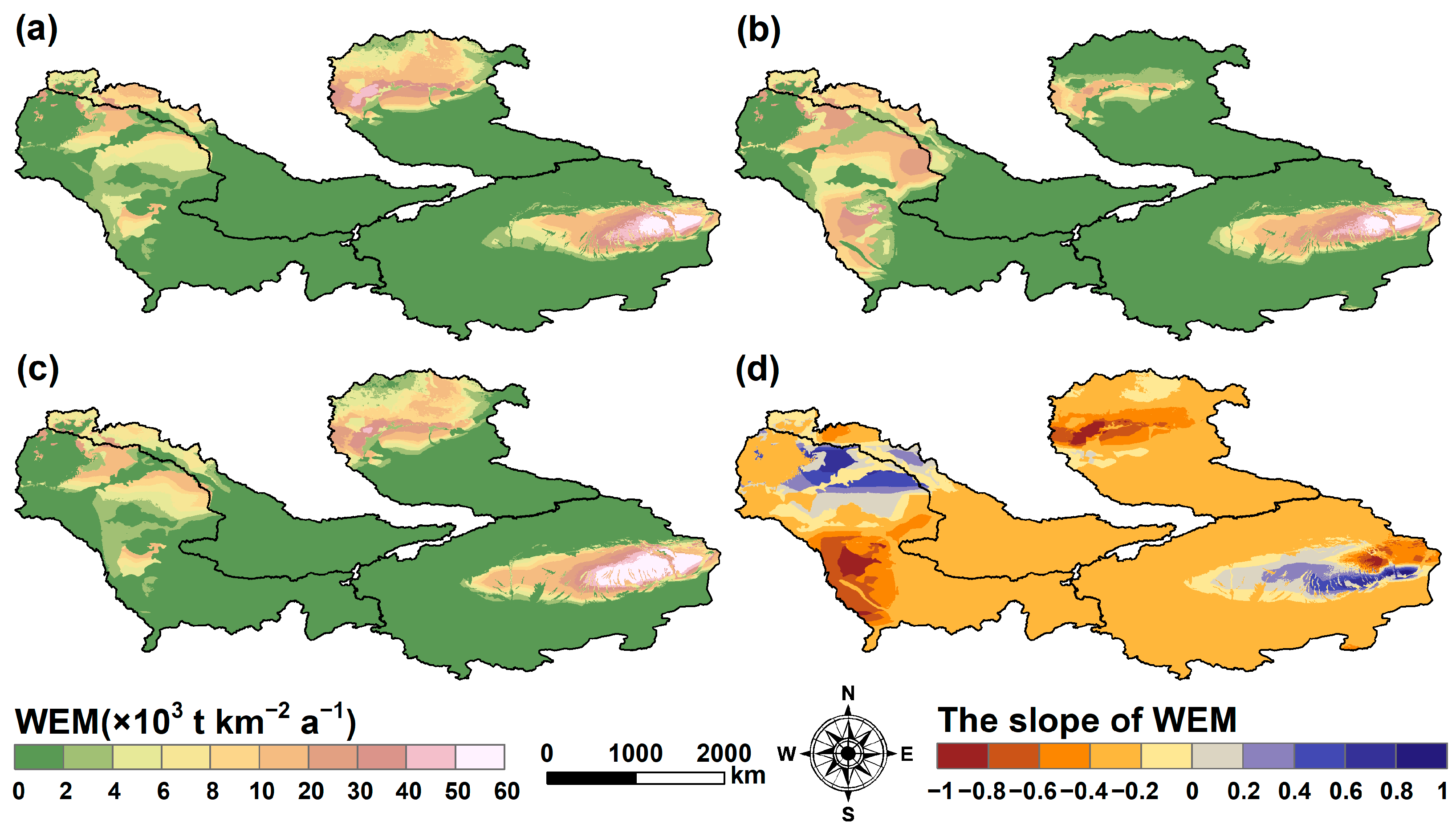
3.1. Spatial Variation of SWE

The variation in SWE within the TLBs in CA is considerable. The WEM ranged from 0 to 60 (10³ t·km⁻²·y⁻¹). Areas with a high WEM of more than 25 (10³ t·km⁻²·y⁻¹) were predominantly identified near the Taklimakan Desert in the TRB, the lower reaches of the IRB close to Lake Balkhash, and the Aral Sea Basin downstream of the SRB and ARB. On the other hand, low WEM areas less than 0.5 (10³ t·km⁻²·y⁻¹) were mainly situated in mountainous regions close to the TLBs in CA, with the Tianshan Mountain range being the most prominent (Figure 2). From 2000 to 2020, the WEM in the downstream areas of the SRB and ARB initially increased and then decreased. Near Lake Balkhash in the downstream IRB, it initially decreased and then increased. In the central and eastern regions of the TRB, the WEM changed from being relatively stable to increasing (Figure 2a–c). In terms of the trend in the spatial variation of the WEM, the regions that exhibited a significant increase in the WEM were mainly located in the central part of the TRB and near the Aral Sea Basin, close to the downstream of the SRB and ARB. The areas where the WEM exhibited a substantial decrease were primarily situated in the vicinity of Lake Balkhash within the IRB and the southern portion of the Kyzylkum Desert in the ARB. For the period spanning two decades (2000–2020), the regions situated within the TLBs in CA where the WEM demonstrated a descending trend in the spatial variation, constituted 71.6% of the entire study area (Figure 2d).

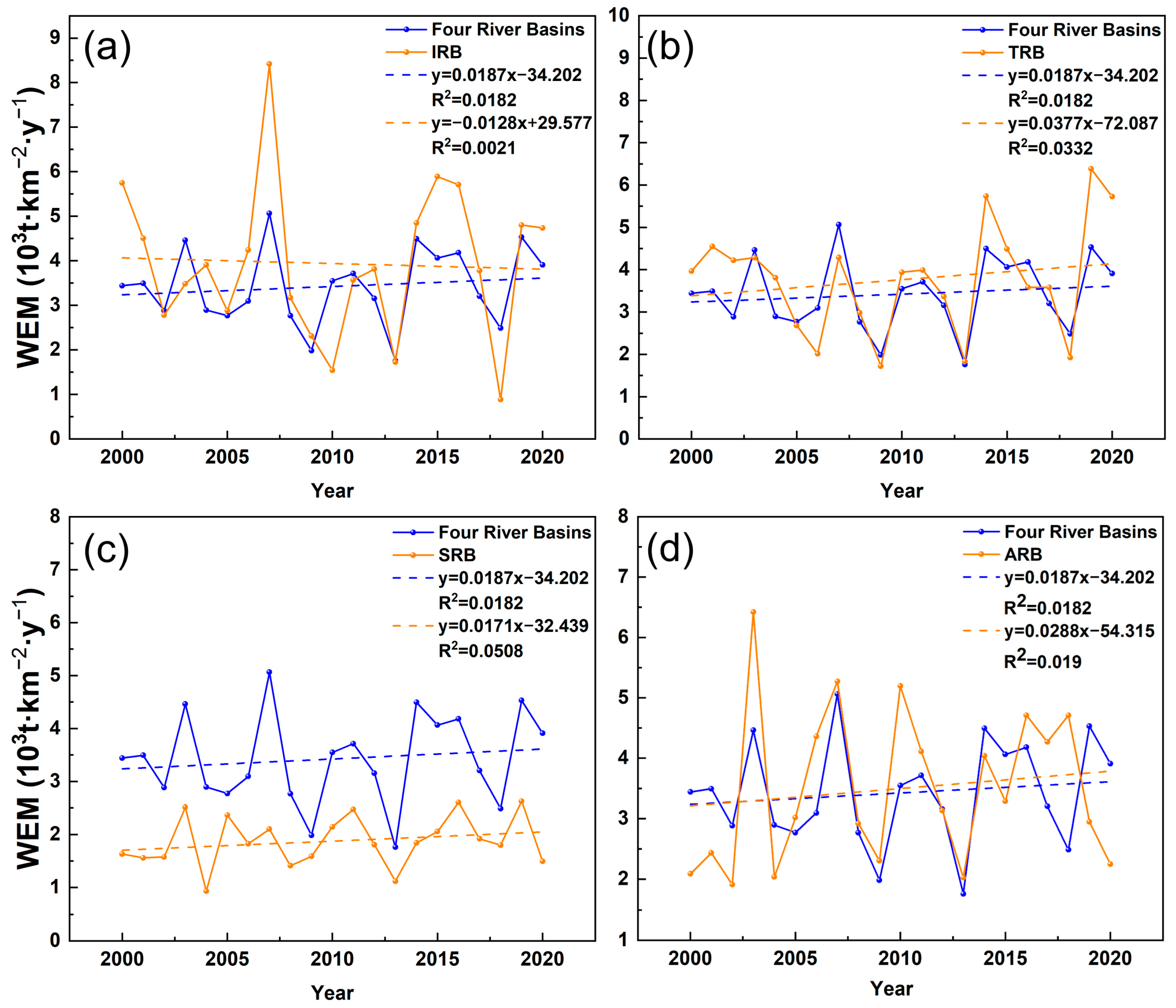
3.2. Temporal Variation of SWE

The temporal variation in the WEM in the TLBs in CA over the past 21 years (2000–2020) was analyzed using a unary linear regression technique. Generally, the TLBs in CA exhibited a fluctuating upward trend, with an average increase of approximately 0.0187 (10³ t·km⁻²·y⁻¹), the peak value was attained in 2007 at 5.06 (10³ t·km⁻²·y⁻¹), followed by a rapid decline to the lowest value in 2009 at 1.98 (10³ t·km⁻²·y⁻¹) (Figure 3). The TRB, SRB, and ARB demonstrated an upward trend in the annual average WEM, the TRB had the most notable upward trend, with an increase of about 0.0377 (10³ t·km⁻²·y⁻¹) (Figure 3b,c). In contrast, the IRB, overall, showed a fluctuating downward trend, with a decrease of about 0.0128 (10³ t·km⁻²·y⁻¹), the highest value was attained in 2007 at 8.42 (10³ t·km⁻²·y⁻¹), followed by a fluctuating downward trend that reached its lowest value in 2018 at 0.86 (10³ t·km⁻²·y⁻¹) (Figure 3a).

3.3. Dust Movement Trajectories

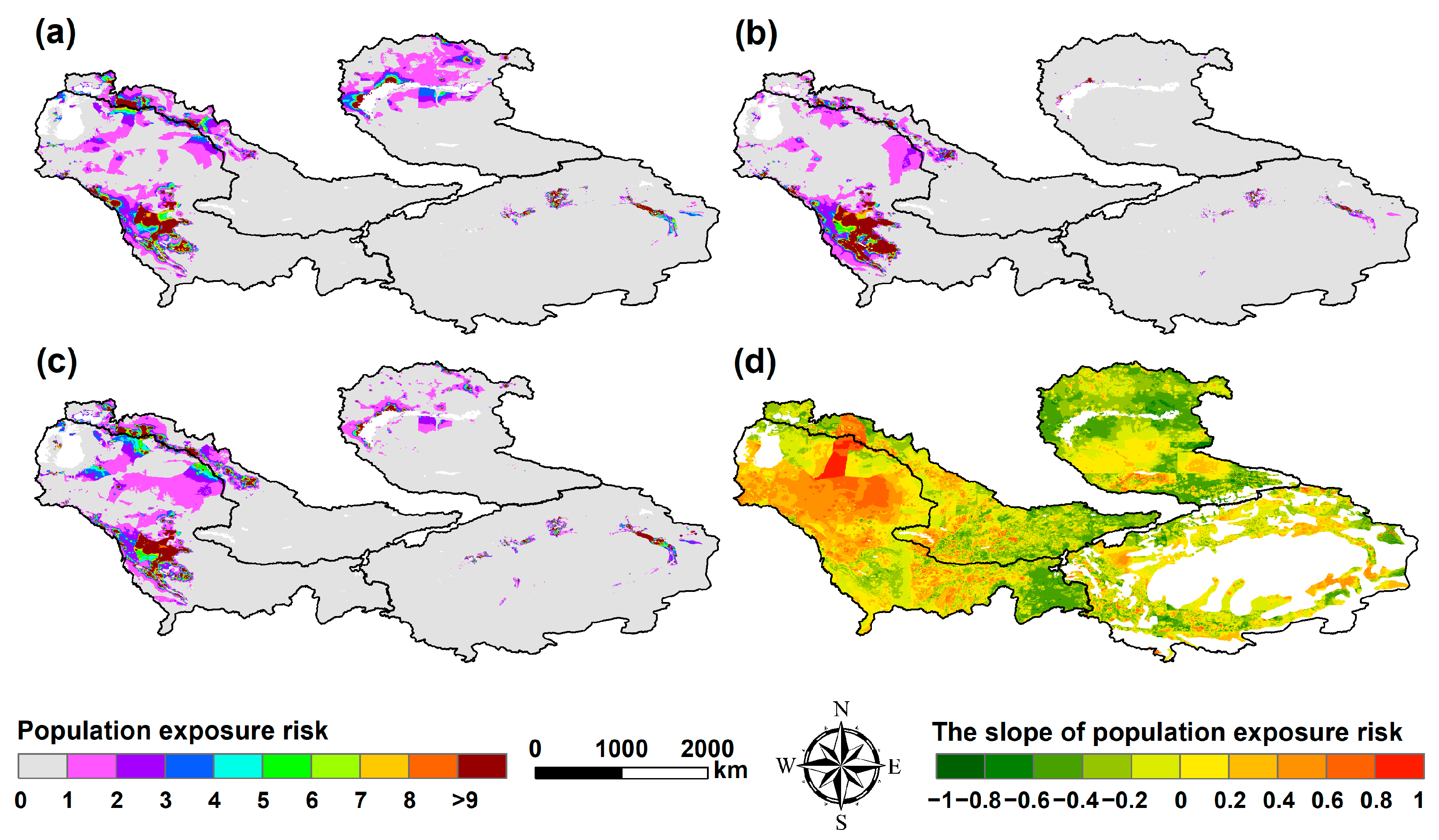
Analysis of the movement trajectories for two typical dust events in the TLBs in CA was conducted (Figure 4). The trajectory at 100 m demonstrated that the dust above the SRB and ARB moved in a westerly direction, passing through regions such as the Black Sea, Russia, Ukraine, and the Caspian Sea. Additionally, the trajectories at 500 m and 1000 m were generally consistent with that at 100 m, reaching the Mediterranean coast (Figure 4a). The dust movement trajectory above the TRB demonstrated a prevalent eastward direction, encompassing extensive regions of northern China and extending as far as the Russian Far East, North Korea, and Japan. Finally, the dust movement trajectories at 100 m and 500 m terminated over the Sea of Japan, whereas the trajectory at 1000 m traverses Japan and ended in the Pacific region (Figure 4b).

3.4. PER to SWE

The PER model was employed to investigate the alterations in the spatial patterns of population exposure risk resulting from SWE in CA (Figure 5). In terms of spatial dispersion, the main areas of PER occurred along the Tarim River, in the vicinity of Lake Balkhash in the lower reaches of the IRB, and in the middle and lower reaches of the ARB and SRB; the high PER areas (>9) were predominantly located in densely populated urban centers and oasis regions (Figure 5a–c). Compared to the year 2000, the most notable reduction in PER around Lake Balkhash in the IRB was observed in 2010, while high PER areas (>9) in the middle reaches of the ARB expanded (Figure 5a,b). From 2010 to 2020, the PER progressively increased in the lower reaches of the IRB and ARB, and new PERs began to emerge in the western and southern parts of the TRB (Figure 5b,c). When comparing the year 2000 to 2020, the PER in the lower reaches of the IRB and ARB areas decreased, while it continuously expanded in the TRB areas (Figure 5a,c). Regarding the spatial change trend, the overall PER in the TLBs in CA demonstrated a decreasing trend, accounting for 55.7% of the entire study area. However, the Aral Sea area exhibited a pronounced increasing trend (Figure 5d).

4. Discussion

4.1. Response of PM2.5 and SWE

PM2.5 is defined as particulate matter with an aerodynamic diameter of less than 2.5 μm [84]. SWE and PM2.5 are interconnected, as the dust generated by this process can be a significant source of airborne particulate matter PM2.5 [85,86]. Agricultural land [87,88] and unpaved roads [89] are potential dust sources in arid and semi-arid regions globally. In central Argentina, SWE has been exacerbated by agricultural and human activities in semi-arid conditions, with poor soil aggregation, high variability in precipitation, and high wind speeds [90,91]. This study conducted spatial correlation analysis between SWE and PM2.5. The research findings indicated that in the IRB, TRB, ARB, and SRB, the regions that exhibited a positive correlation between SWE and PM2.5 account for 46.1%, 34.5%, 36.9%, and 21.6% of the total basin area, respectively, and were mainly distributed in irrigated agricultural areas and rivers (Figure 6). This is consistent with research conducted in Ningxia, China [92], which indicates that SWE of farmland in arid and semi-arid regions can contribute to increased regional PM2.5 concentrations. Meanwhile, a study found that no-till soil can reduce PM2.5 emissions compared to conventionally tilled soil [93]. Therefore, proper no-tillage management practices in the TLBs in CA may reduce PM2.5 emissions in the region and contribute to emergency mitigation and human health in the region.

Li et al. [94] found that the dried-up riverbeds in the Tarim Basin are also a significant source of PM2.5. Concurrently, Li et al. [95] conducted isotope analyses of PM2.5 in the urban regions of Urumqi and found that the composition of atmospheric PM2.5 was consistent with the surface soil of the dried lake bed in the Ebinur Lake area, suggesting that SWE in the lake bed region was the primary cause for the substantial increase in PM2.5. Our study area was the TLBs in CA. As climate change and human activities continue to affect the area, the TLBs have experienced continuous shrinkage. This has led to extensive drying of the riverbed and has been one of the reasons for the significant increase in PM2.5 levels in the region.

4.2. Changes in SWE under Different Land-Use/Cover Changes (LUCCs)

Near-surface wind plays a crucial role in the SWE process, by displacing or removing the top layer of the soil [96]. Furthermore, human activities can affect SWE by changing underlying surface conditions, such as vegetation cover. SWE is highly sensitive to climate change and human-induced LUCCs [97,98,99]. Our study indicated that between 2000 and 2020, there was a significant difference in SWE under different LUCCs in the TLBs in CA (Figure 7). Grasslands and desert lands had higher SWE rates because of the unique topographical and climatic factors of these land-use types [100]. The climate in CA is predominantly arid, primarily consisting of deserts and grasslands. Grasslands cover the largest area and are widespread. Owing to the arid climate in CA, grasslands are currently being severely degraded and are transitioning to deserts [101,102]. The variation in SWE across LUCCs, namely the LUCCs in the study area demonstrated a significant rise in erosion in croplands at +38.00 (10³ t·km⁻²·y⁻¹), forestlands at +100.61 (10³ t·km⁻²·y⁻¹), and desert lands at +557.46 (10³ t·km⁻²·y⁻¹), between 2000 and 2020. In contrast, grasslands at −171.07 (10³ t·km⁻²·y⁻¹) and wetlands at −154.02 (10³ t·km⁻²·y⁻¹) experienced a significant decline (

Table 2. Characteristics of WEM changes under different LUCCs in the TLBs in CA (10³ t·km⁻²·y⁻¹). WEM represents the wind erosion modulus.

Year	Cropland	Forestland	Grassland	Wetland	Construction Land	Desert Land	Others
2000	193.00	1217.47	2240.06	1019.56	1.04	7217.39	0.02
2010	350.10	2099.34	878.95	461.13	2.89	8465.06	0.07
2020	231.00	1318.08	2068.99	865.54	2.41	9022.52	0.02
2000–2010 variation	+157.1	+881.87	−1361.11	−558.43	+1.85	+1247.67	+0.05
2010–2020 variation	−119.1	−781,26	+1190.04	+404.41	−0.48	+680.41	−0.05
2000–2020 variation	+38.00	+100.61	−171.07	−154.02	+1.37	+557.46	0.00

). The substantial increase in SWE in croplands over the past 21 years (2000–2020) in the TLBs in CA may be attributed to extensive land cultivation in the area, with a 15,718.65 km² increase in the cropland region. Consistent with research findings from Inner Mongolia, China, this study indicated that the large-scale expansion of cropland increased SWE [103]. Therefore, more scientific cropland management measures may slow the SWE of cropland in the study area. However, the escalation of SWE in sandy areas may be due to the presence of some of the world’s most extensive mobile deserts (the Taklamakan and Kyzylkum deserts) in the region. These deserts, affected by climate change and human activities, have finer surface soil, leading to increased erodibility [54]. However, our study also revealed that, although some sandy lands have been converted into grassland (Figure 7), this did not hinder the rise in SWE in sandy areas, as severe SWE continued to occur in certain localities. According to Jiang et al. [104], the degree of aridification in CA will remain severe in the future. Considering the continuous expansion of the population and urbanization in the region, this suggests a potential risk of exacerbated SWE in CA in the near future.

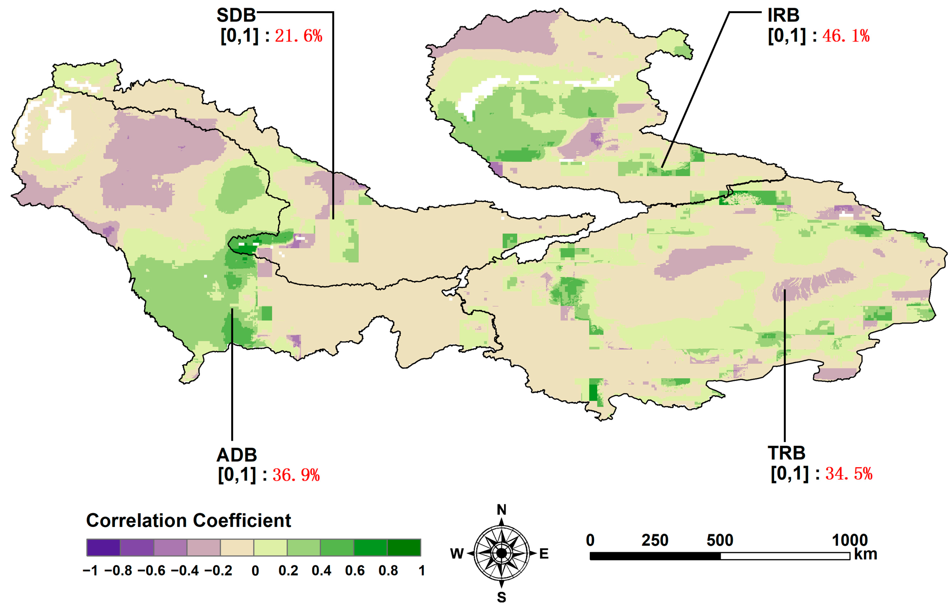
4.3. Relationship between SWE and Controlling Climatic and Vegetation Factors

The climate plays a significant role in the occurrence of SWE, with temperature and precipitation having an indirect influence by affecting soil moisture and vegetation growth [105]. An increase in temperature leads to the increased evaporation of surface water, leading to reduced soil moisture and increased soil erodibility, which in turn increases the likelihood of SWE. We conducted a correlation analysis between SWE and temperature and the results indicated a positive correlation between the two variables in the TLBs in CA (Figure 8a). Specifically, the percentage of the areas with positive correlations within each basin were as follows: IRB (71.7%), TRB (41.9%), ARB (18.6%), and SRB (20.5%). The findings by Ma et al. [22] and Kamali N et al. [106] in global and southwestern Iran context, respectively, indicated that warming led to increased SWE, which is consistent with our results, indicating a positive correlation between rising temperatures and increased SWE. Precipitation is closely linked to the moisture content of surface soil [107]. An increase in soil moisture improves the cohesion between soil particles, thereby strengthening the resistance to SWE [108,109]. Research has demonstrated that precipitation is a critical factor for preventing SWE. Our study discovered that SWE in the TLBs in CA exhibited a negative correlation with precipitation, with the percentage of areas displaying a negative correlation within each basin as follows: IRB (68.7%), TRB (67.5%), ARB (49.5%), and SRB (62.1%) (Figure 8b). These results align with those of Jiang et al. [110] in Inner Mongolia, indicating that increased precipitation played a significant role in reducing regional SWE.

Enhancing vegetation cover is often regarded as a crucial measure for preventing SWE [111]. In desert ecosystems, vegetation can obstruct the flow of windblown sand and improve soil quality. Meng et al. [112] found that vegetation cover inhibited SWE by increasing surface roughness, indicating a negative correlation between vegetation and SWE. Consistent with this perspective, our findings revealed that in a substantial portion of the study area, the NDVI was negatively correlated with SWE. The percentage of negatively correlated areas within the TLBs were as follows: IRB (55%) < ARB (62.1%) < TRB (65.5%) < SRB (78.4%) (Figure 8c). This variation may be attributed to the variability in grassland distribution [113]. Li et al. [114] reported that grassland distribution was the primary cause of spatial differences in SWE in the Xilin Gol grassland in China, as revealed in their study on the impact of SWE. It is worth noting that one study has shown that in arid and semi-arid areas, where water resources are scarce, the construction of windbreaks to increase vegetation cover can effectively reduce SWE and stop land degradation and desertification [3]. Consequently, strengthening grassland management and constructing windbreaks is expected to mitigate SWE in the TLBs in CA.

5. Conclusions

This study used the RWEQ model and PER model to assess SWE and PER in the TLBs in CA from 2000 to 2020. The results showed that: (1) The high SWE areas were mainly concentrated in the Taklamakan Desert, Aral Sea Basin, and near Lake Balkhash, while the PER was primarily located along the Tarim River, near Lake Balkhash, and in the middle and lower reaches of the ARB and SRB. (2) Both SWE and PER show overall decreasing spatial trends. (3) Over time, SWE showed a decreasing trend in the IRB, but an increasing trend in the TRB, SRB, and ARB. (4) The HYSPLIT model demonstrated that dust from the TRB affect large areas in northern China and reach Japan. Dust from the SRB and ARB, downstream of the Aral Sea, ultimately impacts Europe. (5) The driving factors of SWE are as follows: it generally correlates positively with temperature and negatively with precipitation and NDVI. This suggests that increasing temperatures significantly increase SWE in the study area, while increased precipitation and vegetation effectively reduce it. (6) Different LUCCs showed distinct variations in SWE: notably, SWE significantly increased in croplands, forests, and desert areas, while it decreased significantly in grasslands and wetlands.

This study revealed the distribution and variability of SWE and PER in the TLBs in CA, addressing a gap in the research on the relationship between SWE and PER. It also provides theoretical support for emergency mitigation of SWE in arid regions. Enhancing the monitoring of the impact of human activities on SWE and improving the accuracy of the RWEQ model are the future research directions of this study.

References

1. Xu, H.; Wang, Y.; Han, T.; Li, R.; Ma, J.; Qiu, X.; Ying, L.; Zheng, H. Enhanced assessment of regional impacts from wind erosion by integrating particle size. Catena 2024, 239, 107937. [Google Scholar] [CrossRef]
2. Motameni, S.; Soroush, A.; Fattahi, S.M.; Eslami, A. A data-driven approach for assessing the wind-induced erodible fractions of soil. J. Arid. Environ. 2024, 222, 105152. [Google Scholar] [CrossRef]
3. Zhang, H.; Peng, J.; Zhao, C. Wind speed and vegetation coverage in turn dominated wind erosion change with increasing aridity in Africa. Earth’s Future 2024, 12, e2024EF004468. [Google Scholar] [CrossRef]
4. Zou, X.; Li, J.; Cheng, H.; Wang, J.; Zhang, C.; Kang, L.; Liu, W.; Zhang, F. Spatial variation of topsoil features in soil wind erosion areas of northern China. Catena 2018, 167, 429–439. [Google Scholar] [CrossRef]
5. Yan, H.; Wang, S.; Wang, C.; Zhang, G.; Patel, N. Losses of soil organic carbon under wind erosion in China. Glob. Chang. Biol. 2005, 11, 828–840. [Google Scholar] [CrossRef]
6. Zachar, D. Soil Erosion; Elsevier Scientific Publishing Company: Amsterdam, The Netherlands; Oxford, UK; New York, NY, USA, 1982. [Google Scholar] [CrossRef]
7. Chen, L.; Zhao, H.; Han, B.; Bai, Z. Combined use of WEPS and Models-3/CMAQ for simulating wind erosion source emission and its environmental impact. Sci. Total Environ. 2014, 466, 762–769. [Google Scholar] [CrossRef] [PubMed]
8. Mirzabaev, A.; Strokov, A.; Krasilnikov, P. The impact of land degradation on agricultural profits and implications for poverty reduction in Central Asia. Land Use Policy 2023, 126, 106530. [Google Scholar] [CrossRef]
9. Treminio, R.S.; Webb, N.P.; Edwards, B.L.; Faist, A.; Newingham, B.; Kachergis, E. Spatial patterns and controls on wind erosion in the Great Basin. J. Geophys. Res. Biogeosci. 2024, 129, e2023JG007792. [Google Scholar] [CrossRef]
10. Duniway, M.C.; Pfennigwerth, A.A.; Fick, S.E.; Nauman, T.W.; Belnap, J.; Barger, N.N. Wind erosion and dust from US drylands: A review of causes, consequences, and solutions in a changing world. Ecosphere 2019, 10, e02650. [Google Scholar] [CrossRef]
11. Goudarzi, G.; Shirmardi, M.; Naimabadi, A.; Ghadiri, A.; Sajedifar, J. Chemical and organic characteristics of PM2. 5 particles and their in-vitro cytotoxic effects on lung cells: The Middle East dust storms in Ahvaz, Iran. Sci. Total Environ. 2019, 655, 434–445. [Google Scholar] [CrossRef]
12. Marzen, M.; Iserloh, T.; Fister, W.; Seeger, M.; Rodrigo-Comino, J.; Ries, J.B. On-site water and wind erosion experiments reveal relative impact on total soil erosion. Geosciences 2019, 9, 478. [Google Scholar] [CrossRef]
13. Sirjani, E.; Sameni, A.; Mahmoodabadi, M.; Moosavi, A.A.; Laurent, B. In-situ wind tunnel experiments to investigate soil erodibility, soil fractionation and wind-blown sediment of semi-arid and arid calcareous soils. Catena 2024, 241, 108011. [Google Scholar] [CrossRef]
14. Chen, J.; Feng, R.; Li, D.; Yuan, Z. Revealing soil erosion and sediment sources using 137Cs and fingerprinting in an agroforestry catchment. Soil. Tillage Res. 2024, 235, 105919. [Google Scholar] [CrossRef]
15. Pi, H.; Sharratt, B. Evaluation of the RWEQ and SWEEP in simulating soil and PM10 loss from a portable wind tunnel. Soil. Tillage Res. 2017, 170, 94–103. [Google Scholar] [CrossRef]
16. Woodruff, N.P.; Siddoway, F. A wind erosion equation. Soil. Sci. Soc. Am. J. 1965, 29, 602–608. [Google Scholar] [CrossRef]
17. Fryrear, D.; Bilbro, J.; Saleh, A.; Schomberg, H.; Stout, J.; Zobeck, T. RWEQ: Improved wind erosion technology. J. Soil. Water Conserv. 2000, 55, 183–189. [Google Scholar]
18. Hagen, L.J. Evaluation of the Wind Erosion Prediction System (WEPS) erosion submodel on cropland fields. Environ. Model. Softw. 2004, 19, 171–176. [Google Scholar] [CrossRef]
19. Gregory, J.M.; Wilson, G.R.; Singh, U.B.; Darwish, M.M. TEAM: Integrated, process-based wind-erosion model. Environ. Model. Softw. 2004, 19, 205–215. [Google Scholar] [CrossRef]
20. Van Pelt, R.S.; Zobeck, T.M.; Potter, K.N.; Stout, J.E.; Popham, T. Validation of the wind erosion stochastic simulator (WESS) and the revised wind erosion equation (RWEQ) for single events. Environ. Model. Softw. 2004, 19, 191–198. [Google Scholar] [CrossRef]
21. Liao, J.; Peng, F.; Kang, W.; Chen, X.; Sun, J.; Chen, B.; Xia, Y.; Du, H.; Li, S.; Song, X.; et al. No increase of soil wind erosion with the establishment of center pivot irrigation system in Mu-Us sandy land. Sci. Total Environ. 2024, 939, 173558. [Google Scholar] [CrossRef]
22. Ma, X.; Zhao, C.; Zhu, J. Aggravated risk of soil erosion with global warming–A global meta-analysis. Catena 2021, 200, 105129. [Google Scholar] [CrossRef]
23. Duan, W.; Zou, S.; Chen, Y.; Nover, D.; Fang, G.; Wang, Y. Sustainable water management for cross-border resources: The Balkhash Lake Basin of Central Asia, 1931–2015. J. Clean. Prod. 2020, 263, 121614. [Google Scholar] [CrossRef]
24. Wang, J.; Yang, S.; Lou, H.; Liu, H.; Wang, P.; Li, C.; Zhang, F. Impact of lake water level decline on river evolution in Ebinur Lake Basin (an ungauged terminal lake basin). Int. J. Appl. Earth Obs. Geoinf. 2021, 104, 102546. [Google Scholar] [CrossRef]
25. Bolgov, M.; Kashnitskaya, M.; Zaitseva, A.; Pozdnyakov, S.; Ping, W. Long-Term Water Level Fluctuations in Terminal Lakes of Central Asia. Geogr. Nat. Resour. 2022, 43, S15–S21. [Google Scholar] [CrossRef]
26. Deng, H.; Flörke, M.; Lei, K.; Tang, Q. Estimating Multi-sectoral Water Withdrawals Through Machine Learning for Attribution in an Ungauged Terminal Lake Basin in Central Asia. In Proceedings of the EGU General Assembly 2024, Vienna, Austria, 14–19 April 2024. Copernicus Meetings, 2024. [Google Scholar]
27. Dou, X.; Ma, X.; Huo, T.; Zhu, J.; Zhao, C. Assessment of the environmental effects of ecological water conveyance over 31 years for a terminal lake in Central Asia. Catena 2022, 208, 105725. [Google Scholar] [CrossRef]
28. Petr, T.; Mitrofanov, V.P. The impact on fish stocks of river regulation in Central Asia and Kazakhstan. Lakes Reserv. Res. Manag. 1998, 3, 143–164. [Google Scholar] [CrossRef]
29. He, J.; Yu, Y.; Sun, L.; Li, C.; Zhang, H.; Malik, I.; Wistuba, M.; Yu, R. Spatiotemporal variations of ecosystem services in the Aral Sea basin under different CMIP6 projections. Sci. Rep. 2024, 14, 12237. [Google Scholar] [CrossRef] [PubMed]
30. Indoitu, R.; Kozhoridze, G.; Batyrbaeva, M.; Vitkovskaya, I.; Orlovsky, N.; Blumberg, D.; Orlovsky, L. Dust emission and environmental changes in the dried bottom of the Aral Sea. Aeolian Res. 2015, 17, 101–115. [Google Scholar] [CrossRef]
31. Wang, W.; Samat, A.; Abuduwaili, J.; Ge, Y.; De Maeyer, P.; Van de Voorde, T. Temporal characterization of sand and dust storm activity and its climatic and terrestrial drivers in the Aral Sea region. Atmos. Res. 2022, 275, 106242. [Google Scholar] [CrossRef]
32. Breckle, S.-W.; Wucherer, W. The Aralkum, a man-made desert on the desiccated floor of the Aral Sea (Central Asia): Final conclusions and comments. In Aralkum—A Man-Made Desert: The Desiccated Floor of the Aral Sea (Central Asia); Springer: Berlin/Heidelberg, Germany, 2012; pp. 459–464. [Google Scholar] [CrossRef]
33. Khudaybergenov, U.; Abbosov, S.A.; Ollayarov, A. Early Diagnosis and Prevention of Urolithiasis in the Aral Sea Regions. Galaxy Int. Interdiscip. Res. J. 2024, 12, 115–119. [Google Scholar]
34. Goudie, A.S. Desert dust and human health disorders. Environ. Int. 2014, 63, 101–113. [Google Scholar] [CrossRef]
35. Tuholske, C.; Caylor, K.; Funk, C.; Verdin, A.; Sweeney, S.; Grace, K.; Peterson, P.; Evans, T. Global urban population exposure to extreme heat. Proc. Natl. Acad. Sci. USA 2021, 118, e2024792118. [Google Scholar] [CrossRef]
36. Sheldon, L.S.; Cohen Hubal, E.A. Exposure as part of a systems approach for assessing risk. Environ. Health Perspect. 2009, 117, 1181–1194. [Google Scholar] [CrossRef]
37. Zhao, C.; Pan, J.; Zhang, L. Spatio-temporal patterns of global population exposure risk of PM2. 5 from 2000–2016. Sustainability 2021, 13, 7427. [Google Scholar] [CrossRef]
38. Peduzzi, P.; Dao, H.; Herold, C.; Mouton, F. Assessing global exposure and vulnerability towards natural hazards: The Disaster Risk Index. Nat. Hazards Earth Syst. Sci. 2009, 9, 1149–1159. [Google Scholar] [CrossRef]
39. Wang, G.; Yuan, X.; Jing, C.; Hamdi, R.; Ochege, F.U.; Dong, P.; Shao, Y.; Qin, X. The decreased cloud cover dominated the rapid spring temperature rise in arid Central Asia over the period 1980–2014. Geophys. Res. Lett. 2024, 51, e2023GL107523. [Google Scholar] [CrossRef]
40. Bai, J.; Chen, X.; Li, J.; Yang, L.; Fang, H. Changes in the area of inland lakes in arid regions of central Asia during the past 30 years. Environ. Monit. Assess. 2011, 178, 247–256. [Google Scholar] [CrossRef]
41. Deng, H.; Chen, Y. Influences of recent climate change and human activities on water storage variations in Central Asia. J. Hydrol. 2017, 544, 46–57. [Google Scholar] [CrossRef]
42. Jin, C.; Wang, B.; Cheng, T.F.; Dai, L.; Wang, T. How much we know about precipitation climatology over Tianshan Mountains––the Central Asian water tower. npj Clim. Atmos. Sci. 2024, 7, 21. [Google Scholar] [CrossRef]
43. Yang, T.; Chen, X.; Hamdi, R.; Li, Q.; Cui, F.; Li, L.; Liu, Y.; De Maeyer, P.; Duan, W. Assessment of snow simulation using Noah-MP land surface model forced by various precipitation sources in the Central Tianshan Mountains, Central Asia. Atmos. Res. 2024, 300, 107251. [Google Scholar] [CrossRef]
44. Tian, R.; Liu, L.; Zheng, J.; Li, J.; Han, W.; Liu, Y. Combined Effects of Meteorological Factors, Terrain, and Greenhouse Gases on Vegetation Phenology in Arid Areas of Central Asia from 1982 to 2021. Land 2024, 13, 180. [Google Scholar] [CrossRef]
45. Mishra, K.; Choudhary, B.; Fitzsimmons, K.E. Predicting and evaluating seasonal water turbidity in Lake Balkhash, Kazakhstan, using remote sensing and GIS. Front. Environ. Sci. 2024, 12, 1371759. [Google Scholar] [CrossRef]
46. Li, W.; Hao, X.; Chen, Y.; Zhang, L.; Ma, X.; Zhou, H. Response of groundwater chemical characteristics to ecological water conveyance in the lower reaches of the Tarim River, Xinjiang, China. Hydrol. Process. Int. J. 2010, 24, 187–195. [Google Scholar] [CrossRef]
47. Bao, A.; Yu, T.; Xu, W.; Lei, J.; Jiapaer, G.; Chen, X.; Komiljon, T.; Khabibullo, S.; Sagidullaevich, X.B.; Kamalatdin, I. Ecological problems and ecological restoration zoning of the Aral Sea. J. Arid. Land 2024, 16, 315–330. [Google Scholar] [CrossRef]
48. Liu, S.; Long, A.; Yan, D.; Luo, G.; Wang, H. Predicting Ili River streamflow change and identifying the major drivers with a novel hybrid model. J. Hydrol. Reg. Stud. 2024, 53, 101807. [Google Scholar] [CrossRef]
49. Zou, S.; Jilili, A.; Duan, W.; Maeyer, P.D.; de Voorde, T.V. Human and natural impacts on the water resources in the Syr Darya River Basin, Central Asia. Sustainability 2019, 11, 3084. [Google Scholar] [CrossRef]
50. Zan, C.; Liu, T.; Huang, Y.; Bao, A.; Yan, Y.; Ling, Y.; Wang, Z.; Duan, Y. Spatial and temporal variation and driving factors of wetland in the Amu Darya River Delta, Central Asia. Ecol. Indic. 2022, 139, 108898. [Google Scholar] [CrossRef]
51. Feng, M.; Chen, Y.; Li, Z.; Duan, W.; Zhu, Z.; Liu, Y.; Zhou, Y. Optimisation model for sustainable agricultural development based on water-energy-food nexus and CO2 emissions: A case study in Tarim river basin. Energy Convers. Manag. 2024, 303, 118174. [Google Scholar] [CrossRef]
52. Yapiyev, V.; Sagintayev, Z.; Inglezakis, V.J.; Samarkhanov, K.; Verhoef, A. Essentials of endorheic basins and lakes: A review in the context of current and future water resource management and mitigation activities in Central Asia. Water 2017, 9, 798. [Google Scholar] [CrossRef]
53. Bai, J.; Chen, X.; Yang, L.; Fang, H. Monitoring variations of inland lakes in the arid region of Central Asia. Front. Earth Sci. 2012, 6, 147–156. [Google Scholar] [CrossRef]
54. Li, J.; Yuan, X.; Su, Y.; Qian, K.; Liu, Y.; Yan, W.; Xu, S.; Yang, X.; Luo, G.; Ma, X. Trade-offs and synergistic relationships in wind erosion in Central Asia over the last 40 years: A Bayesian Network analysis. Geoderma 2023, 437, 116597. [Google Scholar] [CrossRef]
55. Yang, Y.; Chen, R.-S.; Ding, Y.-J.; Li, H.-Y.; Liu, Z.-W. Changes in global land surface frozen ground and freeze-thaw processes during 1950–2020 based on ERA5-Land data. Adv. Clim. Chang. Res. 2024, 15, 265–274. [Google Scholar] [CrossRef]
56. Wang, Y.-R.; Hessen, D.O.; Samset, B.H.; Stordal, F. Evaluating global and regional land warming trends in the past decades with both MODIS and ERA5-Land land surface temperature data. Remote Sens. Environ. 2022, 280, 113181. [Google Scholar] [CrossRef]
57. Lichiheb, N.; Ngan, F.; Cohen, M. Improving the atmospheric dispersion forecasts over Washington, DC using UrbanNet observations: A study with HYSPLIT model. Urban. Clim. 2024, 55, 101948. [Google Scholar] [CrossRef]
58. Kimo, I.G.; Cholo, B.E.; Lohani, T.K. Identifying the Moisture Sources in Different Seasons for Abaya-Chamo Basin of Southern Ethiopia Using Lagrangian Particle Dispersion Model. Adv. Meteorol. 2024, 2024, 4421766. [Google Scholar] [CrossRef]
59. Ma, J.; Sun, Y.; Meng, D.; Huang, S.; Li, N.; Zhu, H. Accuracy assessment of two global gridded population dataset: A case study in china. In Proceedings of the 4th International Conference on Information Science and Systems, Online, 17–19 March 2021; pp. 120–125. [Google Scholar] [CrossRef]
60. Bhaduri, B. Development of high resolution population and social dynamics models and databases. In Proceedings of the 1st International Conference and Exhibition on Computing for Geospatial Research & Application, Bethesda, MD, USA, 21–23 June 2010; p. 1. [Google Scholar] [CrossRef]
61. Mohanty, M.P.; Simonovic, S.P. Understanding dynamics of population flood exposure in Canada with multiple high-resolution population datasets. Sci. Total Environ. 2021, 759, 143559. [Google Scholar] [CrossRef]
62. Yin, X.; Li, P.; Feng, Z.; Yang, Y.; You, Z.; Xiao, C. Which gridded population data product is better? Evidences from mainland southeast Asia (MSEA). ISPRS Int. J. Geo-Inf. 2021, 10, 681. [Google Scholar] [CrossRef]
63. Albarakat, R.; Lakshmi, V. Comparison of normalized difference vegetation index derived from Landsat, MODIS, and AVHRR for the Mesopotamian marshes between 2002 and 2018. Remote Sens. 2019, 11, 1245. [Google Scholar] [CrossRef]
64. Wang, S.; Liu, Q.; Huang, C. Vegetation change and its response to climate extremes in the arid region of Northwest China. Remote Sens. 2021, 13, 1230. [Google Scholar] [CrossRef]
65. Hao, H.; Chen, Y.; Xu, J.; Li, Z.; Li, Y.; Kayumba, P.M. Water deficit may cause vegetation browning in central Asia. Remote Sens. 2022, 14, 2574. [Google Scholar] [CrossRef]
66. Fan, J.; Fan, Y.; Cheng, J.; Wu, H.; Yan, Y.; Zheng, K.; Shi, M.; Yang, Q. The Spatio-Temporal Evolution Characteristics of the Vegetation NDVI in the Northern Slope of the Tianshan Mountains at Different Spatial Scales. Sustainability 2023, 15, 6642. [Google Scholar] [CrossRef]
67. Wang, S.; Cui, D.; Wang, L.; Peng, J. Applying deep-learning enhanced fusion methods for improved NDVI reconstruction and long-term vegetation cover study: A case of the Danjiang River Basin. Ecol. Indic. 2023, 155, 111088. [Google Scholar] [CrossRef]
68. Xu, S.; Su, Y.; Yan, W.; Liu, Y.; Wang, Y.; Li, J.; Qian, K.; Yang, X.; Ma, X. Influences of Ecological Restoration Programs on Ecosystem Services in Sandy Areas, Northern China. Remote Sens. 2023, 15, 3519. [Google Scholar] [CrossRef]
69. Guida, G.; Nicosia, A.; Settanni, L.; Ferro, V. A review on effects of biological soil crusts on hydrological processes. Earth-Sci. Rev. 2023, 243, 104516. [Google Scholar] [CrossRef]
70. Chamizo, S.; Rodríguez-Caballero, E.; Cantón, Y.; Asensio, C.; Domingo, F. Penetration resistance of biological soil crusts and its dynamics after crust removal: Relationships with runoff and soil detachment. Catena 2015, 126, 164–172. [Google Scholar] [CrossRef]
71. Xu, J.; Xiao, Y.; Xie, G.; Wang, Y.; Jiang, Y. Computing payments for wind erosion prevention service incorporating ecosystem services flow and regional disparity in Yanchi County. Sci. Total Environ. 2019, 674, 563–579. [Google Scholar] [CrossRef]
72. Wang, S.; Shi, H.; Xu, X.; Huang, L.; Gu, Q.; Liu, H. County zoning and optimization paths for trade-offs and synergies of ecosystem services in Northeast China. Ecol. Indic. 2024, 164, 112044. [Google Scholar] [CrossRef]
73. Huang, D.; Zhang, Y.; Cheng, H.; Andrea, C.; Shi, J.; Chen, C.; Teng, Y.; Zeng, L. Evaluating air pollution exposure among cyclists: Real-time levels of PM2.5 and NO2 and POI impact. Sci. Total Environ. 2024, 945, 173559. [Google Scholar] [CrossRef] [PubMed]
74. Stein, A.; Draxler, R.R.; Rolph, G.D.; Stunder, B.J.; Cohen, M.D.; Ngan, F. NOAA’s HYSPLIT atmospheric transport and dispersion modeling system. Bull. Am. Meteorol. Soc. 2015, 96, 2059–2077. [Google Scholar] [CrossRef]
75. Qor-el-aine, A.; Beres, A.; Geczi, G. Dust storm simulation over the Sahara Desert (Moroccan and Mauritanian regions) using HYSPLIT. Atmos. Sci. Lett. 2022, 23, e1076. [Google Scholar] [CrossRef]
76. Gammoudi, N.; Kovács, J.; Gresina, F.; Varga, G. Combined use of HYSPLIT model and MODIS aerosols optical depth to study the spatiotemporal circulation patterns of Saharan dust events over Central Europe. Aeolian Res. 2024, 67, 100899. [Google Scholar] [CrossRef]
77. Alebić-Juretić, A.; Mifka, B.; Kuzmić, J. Airborne desert dust in the Northern Adriatic area (Croatia): Different sources. Sci. Total Environ. 2024, 912, 169320. [Google Scholar] [CrossRef] [PubMed]
78. Miao, M.; Zhang, M.; Wang, S.; Sun, Z.; Li, X.; Yuan, X.; Yang, G.; Hu, Z.; Zhang, S. Effect of oasis and irrigation on mountain precipitation in the northern slope of Tianshan Mountains based on stable isotopes. J. Hydrol. 2024, 635, 131151. [Google Scholar] [CrossRef]
79. Mao, X.; Xing, L.; Shang, W.; Li, S.; Duan, K. Moisture sources for precipitation over the Pamirs Plateau in winter and spring. Q. J. R. Meteorol. Soc. 2024, 150, 820–833. [Google Scholar] [CrossRef]
80. Endale, T.A.; Raba, G.A.; Beketie, K.T.; Feyisa, G.L.; Gebremichael, H.B. Assessment of particulate matter and particle path trajectory analysis using a HYSPLIT model over Dire Dawa, Ethiopia. Discov. Appl. Sci. 2024, 6, 131. [Google Scholar] [CrossRef]
81. Hwang, H.; Lee, J.E.; Shin, S.A.; You, C.R.; Shin, S.H.; Park, J.-S.; Lee, J.Y. Vertical Profiles of PM2. 5 and O3 Measured Using an Unmanned Aerial Vehicle (UAV) and Their Relationships with Synoptic-and Local-Scale Air Movements. Remote Sens. 2024, 16, 1581. [Google Scholar] [CrossRef]
82. Zhang, S.; Wang, Y.; Zhang, C.; Wu, Y.; Li, C.; Yin, Y. Response mechanism of the thermal environment in the karst rocky desertification areas from the perspective of settlement transition. Urban. Clim. 2024, 55, 101984. [Google Scholar] [CrossRef]
83. Tuoku, L.; Wu, Z.; Men, B. Impacts of climate factors and human activities on NDVI change in China. Ecol. Inform. 2024, 81, 102555. [Google Scholar] [CrossRef]
84. Panebianco, J.E.; Mendez, M.J.; Buschiazzo, D.E. PM10 emission, sandblasting efficiency and vertical entrainment during successive wind-erosion events: A wind-tunnel approach. Bound.-Layer Meteorol. 2016, 161, 335–353. [Google Scholar] [CrossRef]
85. Li, J.-d.; Deng, Q.-h.; Lu, C.; Huang, B.-l. Chemical compositions and source apportionment of atmospheric PM10 in suburban area of Changsha, China. J. Cent. South Univ. Technol. 2010, 17, 509–515. [Google Scholar] [CrossRef]
86. Bi, X.; Feng, Y.; Wu, J.; Wang, Y.; Zhu, T. Source apportionment of PM10 in six cities of northern China. Atmos. Environ. 2007, 41, 903–912. [Google Scholar] [CrossRef]
87. Zobeck, T.M.; Van Pelt, R.S. Wind-induced dust generation and transport mechanics on a bare agricultural field. J. Hazard. Mater. 2006, 132, 26–38. [Google Scholar] [CrossRef] [PubMed]
88. Kjelgaard, J.; Sharratt, B.; Sundram, I.; Lamb, B.; Claiborn, C.; Saxton, K.; Chandler, D. PM10 emission from agricultural soils on the Columbia Plateau: Comparison of dynamic and time-integrated field-scale measurements and entrainment mechanisms. Agric. For. Meteorol. 2004, 125, 259–277. [Google Scholar] [CrossRef]
89. Goossens, D.; Buck, B. Effects of wind erosion, off-road vehicular activity, atmospheric conditions and the proximity of a metropolitan area on PM10 characteristics in a recreational site. Atmos. Environ. 2011, 45, 94–107. [Google Scholar] [CrossRef]
90. Buschiazzo, D.E.; Zobeck, T.M.; Aimar, S.B. Wind erosion in loess soils of the Semiarid Argentinian Pampas. Soil. Sci. 1999, 164, 133–138. [Google Scholar] [CrossRef]
91. Colazo, J.C.; Buschiazzo, D.E. Soil dry aggregate stability and wind erodible fraction in a semiarid environment of Argentina. Geoderma 2010, 159, 228–236. [Google Scholar] [CrossRef]
92. Tian, M.; Gao, J.; Zhang, L.; Zhang, H.; Feng, C.; Jia, X. Effects of dust emissions from wind erosion of soil on ambient air quality. Atmos. Pollut. Res. 2021, 12, 101108. [Google Scholar] [CrossRef]
93. Li, H.; Tatarko, J.; Kucharski, M.; Dong, Z. PM2. 5 and PM10 emissions from agricultural soils by wind erosion. Aeolian Res. 2015, 19, 171–182. [Google Scholar] [CrossRef]
94. Li, X.; Feng, G.; Zhao, C.; Zheng, Z. Land degradation potential by soil erosion under different land uses in the dry area of Tarim Basin. In Global Climate Change and Its Impact on Food & Energy Security in the Drylands, Proceedings of the Eleventh International Dryland Development Conference, Beijing, China, 18–21 March 2013; International Dryland Development Commission (IDDC): Cairo, Egypt, 2014. [Google Scholar]
95. Li, Y.; Ma, L.; Ge, Y.; Abuduwaili, J. Health risk of heavy metal exposure from dustfall and source apportionment with the PCA-MLR model: A case study in the Ebinur Lake Basin, China. Atmos. Environ. 2022, 272, 118950. [Google Scholar] [CrossRef]
96. Zhao, C.; Zhang, H.; Wang, M.; Jiang, H.; Peng, J.; Wang, Y. Impacts of climate change on wind erosion in Southern Africa between 1991 and 2015. Land Degrad. Dev. 2021, 32, 2169–2182. [Google Scholar] [CrossRef]
97. Zhao, Y.; Wu, J.; He, C.; Ding, G. Linking wind erosion to ecosystem services in drylands: A landscape ecological approach. Landsc. Ecol. 2017, 32, 2399–2417. [Google Scholar] [CrossRef]
98. Tegen, I.; Lacis, A.A.; Fung, I. The influence on climate forcing of mineral aerosols from disturbed soils. Nature 1996, 380, 419–422. [Google Scholar] [CrossRef]
99. Pi, H.; Sharratt, B.; Feng, G.; Lei, J. Evaluation of two empirical wind erosion models in arid and semi-arid regions of China and the USA. Environ. Model. Softw. 2017, 91, 28–46. [Google Scholar] [CrossRef]
100. Klein, I.; Gessner, U.; Kuenzer, C. Regional land cover mapping and change detection in Central Asia using MODIS time-series. Appl. Geogr. 2012, 35, 219–234. [Google Scholar] [CrossRef]
101. Jiang, J.; Zhou, T.; Chen, X.; Wu, B. Central Asian precipitation shaped by the tropical Pacific decadal variability and the Atlantic multidecadal variability. J. Clim. 2021, 34, 7541–7553. [Google Scholar] [CrossRef]
102. Chen, F.; Huang, W.; Jin, L.; Chen, J.; Wang, J. Spatiotemporal precipitation variations in the arid Central Asia in the context of global warming. Sci. China Earth Sci. 2011, 54, 1812–1821. [Google Scholar] [CrossRef]
103. Chi, W.; Zhao, Y.; Kuang, W.; Pan, T.; Ba, T.; Zhao, J.; Jin, L.; Wang, S. Impact of cropland evolution on soil wind erosion in Inner Mongolia of China. Land 2021, 10, 583. [Google Scholar] [CrossRef]
104. Jiang, J.; Zhou, T.; Chen, X.; Zhang, L. Future changes in precipitation over Central Asia based on CMIP6 projections. Environ. Res. Lett. 2020, 15, 054009. [Google Scholar] [CrossRef]
105. Sharratt, B.; Tatarko, J.; Abatzoglou, J.; Fox, F.; Huggins, D. Implications of climate change on wind erosion of agricultural lands in the Columbia plateau. Weather. Clim. Extrem. 2015, 10, 20–31. [Google Scholar] [CrossRef]
106. Kamali, N.; Siroosi, H.; Sadeghipour, A. Impacts of wind erosion and seasonal changes on soil carbon dioxide emission in southwestern Iran. J. Arid. Land 2020, 12, 690–700. [Google Scholar] [CrossRef]
107. Koster, R.D.; Suarez, M.J.; Higgins, R.W.; Van den Dool, H.M. Observational evidence that soil moisture variations affect precipitation. Geophys. Res. Lett. 2003, 30, 45. [Google Scholar] [CrossRef]
108. Bergametti, G.; Rajot, J.-L.; Pierre, C.; Bouet, C.; Marticorena, B. How long does precipitation inhibit wind erosion in the Sahel? Geophys. Res. Lett. 2016, 43, 6643–6649. [Google Scholar] [CrossRef]
109. Seneviratne, S.I.; Corti, T.; Davin, E.L.; Hirschi, M.; Jaeger, E.B.; Lehner, I.; Orlowsky, B.; Teuling, A.J. Investigating soil moisture–climate interactions in a changing climate: A review. Earth-Sci. Rev. 2010, 99, 125–161. [Google Scholar] [CrossRef]
110. Jiang, L.; Xiao, Y.; Zheng, H.; Ouyang, Z. Spatio-temporal variation of wind erosion in Inner Mongolia of China between 2001 and 2010. Chin. Geogr. Sci. 2016, 26, 155–164. [Google Scholar] [CrossRef]
111. Chi, W.; Zhao, Y.; Kuang, W.; He, H. Impacts of anthropogenic land use/cover changes on soil wind erosion in China. Sci. Total Environ. 2019, 668, 204–215. [Google Scholar] [CrossRef]
112. Meng, Z.; Dang, X.; Gao, Y.; Ren, X.; Ding, Y.; Wang, M. Interactive effects of wind speed, vegetation coverage and soil moisture in controlling wind erosion in a temperate desert steppe, Inner Mongolia of China. J. Arid. Land 2018, 10, 534–547. [Google Scholar] [CrossRef]
113. Wang, G.; Wanquan, T.; Mingyuan, D. Flux and composition of wind-eroded dust from different landscapes of an arid inland river basin in north-western China. J. Arid. Environ. 2004, 58, 373–385. [Google Scholar] [CrossRef]
114. Li, Z.; Wei, J.; Hao, R. The constraint effect of grassland vegetation on soil wind erosion in Xilin Gol of China. Ecol. Indic. 2023, 155, 111006. [Google Scholar] [CrossRef]
Figure 1. Overview map of the TLBs in CA. IRB represents the Ili River Basin, TRB represents the Tarim River Basin, SRB represents the Syr Darya River Basin, and ARB represents the Amu Darya River Basin.
Water 16 01911 g001
Figure 2. Spatial distribution and trend changes in SWE in the TLBs in CA: (ac) represent the spatial distribution maps of SWE in the TLBs in CA for 2000, 2010, and 2020, respectively; (d) shows the spatial trend changes in SWE in the TLBs in CA from 2000 to 2020. WEM represents the wind erosion modulus.
Water 16 01911 g002
Figure 3. Temporal changes in SWE in the TLBs in CA from 2000 to 2020: (ad) represent the temporal changes in SWE in the IRB, TRB, SRB, and ARB, respectively, from 2000 to 2020. IRB represents the Ili River Basin, TRB represents the Tarim River Basin, SRB represents the Syr Darya River Basin, and ARB represents the Amu Darya River Basin. WEM represents the wind erosion modulus.
Water 16 01911 g003
Figure 4. Simulation map of the forward trajectory of dust following two typical dust events in the TLBs in CA. Specifically, (a) represents the 72 h dust movement trajectory at altitudes of 100 m (red), 500 m (blue), and 1000 m (green) above the SRB and ARB at 0:00 Coordinated Universal Time (UTC) on 24 March 2020; (b) represents the 72 h dust movement trajectory at altitudes of 100 m (red), 500 m (blue), and 1000 m (green) above the Tarim River Basin (TRB) at 0:00 UTC on 2 April 2018. Based on two typical dust events, the spatial dynamic movement trajectory of the SWE in the study area can be more clearly understood.
Water 16 01911 g004
Figure 5. Spatial distribution and trend map of PER in the TLBs in CA: (ac) represent the spatial distribution maps of PER in the TLBs in CA for 2000, 2010, and 2020, respectively; (d) represents the spatial trend changes in the PER in the TLBs in CA from 2000 to 2020.
Water 16 01911 g005
Figure 6. Spatial correlation between SWE and PM2.5 in the TLBs in CA. Basin abbreviations: IRB (Ili River Basin), TRB (Tarim River Basin), SRB (Syr Darya River Basin), and ARB (Amu Darya River Basin). WEM represents the wind erosion modulus. The brackets indicate the percentage of the area within each basin that showed a positive correlation.
Water 16 01911 g006
Figure 7. Chord diagram of changes in different LUCCs in the TLBs in CA from 2000 to 2020. K is the letter form of the measurement unit, which represents a thousand units.
Water 16 01911 g007
Figure 8. Spatial correlation maps of SWE with temperature (a), precipitation (b), and NDVI (c) in the TLBs in CA. IRB, Ili River Basin; TRB, Tarim River Basin; SRB, Syr Darya Basin; ARB, Amu Darya Basin. The brackets indicate the percentage of the area within each basin that showed a positive correlation.
Water 16 01911 g008