Numerical Study on the Influence of Installation Height and Operating Frequency of Biomimetic Pumps on the Incipient Motion of Riverbed Sediment

Abstract

Biomimetic pumps can effectively enhance the hydrodynamics of plain river networks, improve the water environment, and facilitate the transport of sticky bottom sediment. In this paper, a biomimetic pump equipped with an NACA0012 wing profile was used as the research subject, and a commercial CFD package was employed to investigate the impact of the pump’s installation height (the vertical distance from the hydrofoil’s pivot to the riverbed) and operating frequency on the incipient motion of riverbed sediment. The results indicate that the lowest maximum near-bed velocity is obtained at an installation height of 3 times the chord length (3 c) and operating frequency of 0.5 Hz, while the highest is reached at 4 c and 5 Hz. The maximum near-bed velocity point is the furthest from the biomimetic pump when the installation height is 3 c and the operating frequency is 0.5 Hz and the closest at 4 c and 0.5 Hz. At a fixed installation height, a quadratic relationship is found between the maximum near-bed velocity and the operating frequency. At installation heights of c, 2 c, and 4 c, the effect of operating frequency on the point of action is minimal, with only a sudden change followed by stability at 3 c as the frequency increases. When the operating frequency is fixed and the installation height is increased, the maximum near-bed velocity initially decreases and then rises, being the smallest at 3 c. The distance between the point of maximum near-bed velocity and the biomimetic pump initially increases and then decreases with increasing installation height, being the farthest at 3 c. Furthermore, in this paper, we fitted mathematical expressions for the maximum near-bed velocity relative to the operating frequency under different installation heights of the biomimetic pump and calculated the threshold frequencies for the incipient motion of sediment at installation heights of c, 2 c, 3 c, and 4 c to be 1.15 Hz, 1.64 Hz, 2.85 Hz, and 1.06 Hz, respectively, providing scientific guidance for the application of biomimetic pumps in various scenarios.

1. Introduction

In the vast river network regions of southern China, the issue of water environmental degradation caused by a scarcity of hydraulic power is widespread [1,2]. Although diversion and pumping projects combined with pump gate joint control technology can enhance hydraulic power and improve water quality to some extent, their efficiency often appears limited under ultra-low head conditions, rendering them ineffective [3,4,5]. The studies in [6,7] have indicated that the use of flapping biomimetic pumps designed with bionic principles, which mimic the oscillation characteristics of fish tails, offers some advantages, such as having a simple structure, a low head, and a high efficiency. This makes them more suitable for improving hydraulic power in small channels under ultra-low head conditions. In urban river networks, the biomimetic pump can adjust the water velocity through parameter modifications. However, such adjustments may induce the incipient motion of riverbed sediment. During the daytime, fine-tuning the operational parameters of the biomimetic pump can increase the water velocity without disturbing any sediment, keeping the water clear. On the other hand, at night, appropriate adjustments to the operating parameters can stimulate effective scouring of the bottom sediment, contributing to a reduction in riverbed silt, thereby enhancing the river channel’s water environment. In this study, we take this practical need as its backdrop, focusing on the impact of the biomimetic pump on the incipient motion of riverbed sediment.

Biomimetic pumps utilize the propulsion characteristics of biomimetic hydrofoils to perform water-pushing tasks. Many researchers have conducted in-depth studies aimed at enhancing the propulsion performance of biomimetic hydrofoils. Lin et al. [8] employed numerical methods to investigate the propulsion performance of an underwater vehicle with span-wise curved hydrofoils, noting that a span-wise curvature significantly affects the vortex evolution and wake structure, and revealed that adjusting the curvature parameters and phase can effectively enhance the propulsion effect of flapping foils. By adjusting the parameters, the propulsion performance can be maximized to achieve a thrust increase of 137% and an efficiency improvement of 111% compared to rigid foils. Du et al. [9] used numerical simulation techniques to comparatively analyze the effects of four different motion modes of underwater flapping foils on propulsion performance and flow field structure. It is concluded that the maximum average thrust is generated when the flapping wing has the maximum pitch angle at the initial position and the directions of the heaving motion and pitching motion of the wing are the same. Ding et al. [10] utilized numerical simulation methods to reveal the thrust generation mechanism of underwater flapping foils and the relationship between motion parameters and propulsion efficiency. The study also presented the variation curves of propulsion efficiency with motion parameters for underwater flapping wings, including the optimal propulsion efficiency point. Li et al. [11] adopted numerical simulation methods to explore the impact of non-sinusoidal motion on the propulsion performance of tandem hydrofoils. Under certain conditions, non-sinusoidal motion can enhance the propulsion efficiency of both the front and rear foils. Hua et al. [6,7,12,13] conducted in-depth studies on the effects of motion patterns, pivot positions, and flow channel structures of biomimetic flapping foils on propulsion performance and flow field through a combination of numerical simulations and experimentation. The results indicate that, with motion parameters held constant, a decrease in flow channel width corresponds to an increase in outlet velocity, lift, and efficiency of the device, while simultaneously reducing the flow rate. In ultra-low head conditions, the hydrofoil with a positive arc flapping mechanism outperforms the traditional linear flapping hydrofoil in pumping capabilities. As the pivot point shifts towards the trailing edge, the water pushing efficiency experiences an initial rise followed by a decline. Notably, the water pushing efficiency reaches its peak when the pivot is positioned at 0.2 times the chord length from the leading edge. Li et al. [14] discussed the propulsion characteristics of NACA012 hydrofoils based on fish kinematics under non-sinusoidal motion via a numerical simulation. The findings indicate that non-sinusoidal trajectories influence propulsion performance by modifying the angle of attack (AOA), altering the hydrodynamic characteristics of the foil, and changing the flow pattern behind the foil. In comparison to sinusoidal motions, non-sinusoidal flapping trajectories can substantially enhance the thrust coefficient at identical kinematic parameters in most instances. Nevertheless, they might diminish propulsive efficiency. Zhou et al. [15] used numerical simulation methods to investigate the working characteristics and hydrodynamic performance of semi-active oscillating foils driven by a swing arm. The findings indicate that extending the swing arm length positively impacts both the peak efficiency of the flapping foil and enhances the thrust coefficient at the peak efficiency point. The maximum angle of attack is identified as a pivotal factor that influences the performance of this flapping foil propulsion system. Mei et al. [16] carried out systematic parametric studies, comparing and analyzing sinusoidal and non-sinusoidal underwater flapping propulsion systems, clearly indicating that the amplitude of heave has a significant impact on propulsion efficiency. Notably, they found that the optimal efficiency could attain values as high as 87% when the heave amplitude-to-chord ratio is 3.0. They also point out that phase differences affect efficiency, although its specific mechanism requires further investigation. The current research on biomimetic pumps primarily focuses on enhancing the propulsion performance of biomimetic hydrofoils to improve the water-pumping capacity of the pumps, yet the study of their impact on riverbed sediment during operation is not yet sufficiently thorough.

Sediments in plain river networks primarily consist of fine particulate matter. In terms of sediment incipient motion, Yang et al. [17] utilized experimental measurements to determine the incipient velocity of fine-grained sediment at the Yong River estuary and revised the sediment incipient motion formula proposed by Dou Guoren, thereby obtaining a formula suitable for the incipient velocity of cohesive fine sediment under both deep and shallow water conditions. Zhou et al. [18] found, through experiments, that the consolidation degree of cohesive lakebed silt in Poyang Lake varies with different stages as the duration of deposition increases and established an empirical formula for incipient velocity related to deposition duration and water depth. Sun et al. [19], based on a formula for the initiation of motion frictional velocity for cohesive non-uniform sediment that was proposed from a probabilistic and mechanical perspective, established formulas for the initiation of motion velocity and the erosion rate of cohesive non-uniform sediment and verified their accuracy through experimentation. Xiao et al. [20] collected sediment samples from the marine area of the Zhejiang Cangnan Power Plant and, through indoor flume tests, discovered that the incipient velocity of sticky silt under the combined action of waves and currents or pure wave action is significantly lower than that under pure current flow and that the incipient velocity increases with the wet unit weight of the bottom sediment.

To thoroughly understand the impact of a biomimetic pump operation on riverbed sediment, establishing a benchmark for sediment incipient motion is crucial. Given that current research focuses on incipient velocity, in this paper, we adopt the near-bed incipient velocity of cohesive sediment as the standard, using the average bottom velocity at the initiation of motion of the surface sediment beneath Yubu Bridge in Jiaxing City, Zhejiang Province, as the critical incipient velocity for sediment. Since only the installation height and operating frequency can be adjusted post-fabrication of the biomimetic pump, we use the biomimetic pump based on the NACA0012 airfoil profile developed by the Intelligent Design and Manufacturing Laboratory at Zhejiang University of Technology as an example, employing numerical simulation methods to examine the relationship between the biomimetic pump’s operation at various installation heights and operating frequencies and the incipient motion of riverbed sediment. The aim is to provide scientific guidance for the application of biomimetic pumps in different urban river network scenarios.

2. Working Principle and Geometric Model of Biomimetic Pumps

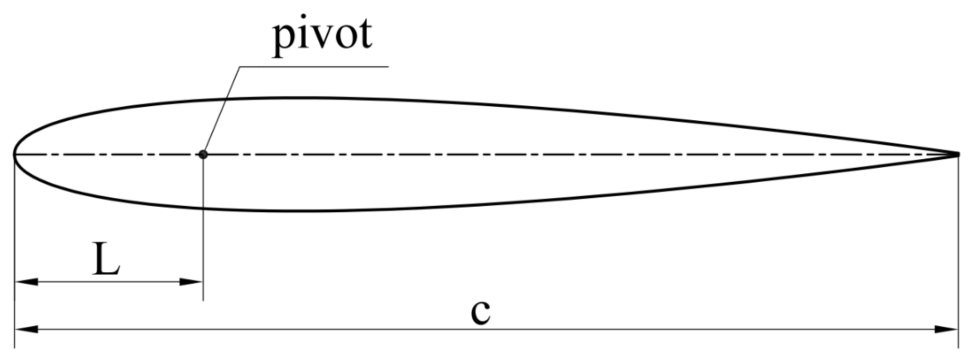
2.1. Geometric Model of Biomimetic Hydrofoils

This paper focuses on the study of biomimetic pumps equipped with NACA0012 airfoil profiles. Figure 1 provides a structural schematic of the NACA0012 airfoil. The simulation results of the hydrofoil in both 3D and 2D are found to be nearly identical, with negligible impact from the three-dimensional effect. To optimize computational resources, this study adopts a two-dimensional hydrofoil model.

In the figure, c denotes the chord length of the biomimetic hydrofoil. In this study, the chord length c is set at 0.3 m. L is the distance from the pivot axis to the leading edge of the biomimetic hydrofoil, which, following that used in [12], is taken as L = 0.2 c. The pivot axis serves as the center point for the combined motion of the biomimetic hydrofoil.

The installation height of the biomimetic pump is defined as the distance between the pivot axis and the riverbed when the biomimetic hydrofoil is at the center of its heaving motion, as illustrated in Figure 2.

In the figure, H denotes the installation height of the biomimetic pump.

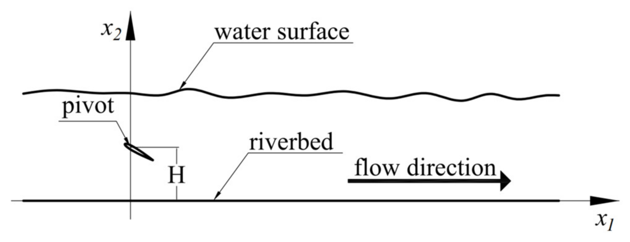
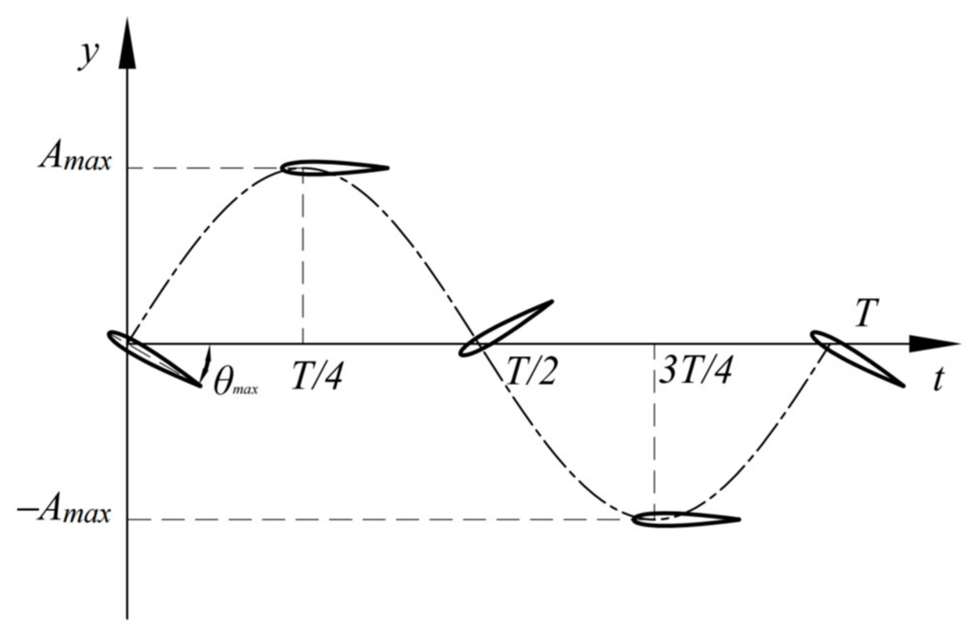
2.2. Working Principle of Biomimetic Pumps

A biomimetic pump is a water-pumping apparatus that employs the propulsive attributes of biomimetic hydrofoils, which mimic the undulation of fish tails to perform highly efficient water propulsion. The motion of the biomimetic hydrofoils involves a combination of heaving (vertical lifting) and pitching (rotational) movements. Figure 3 provides a schematic representation of the biomimetic hydrofoil motion.

The equation for the motion of a biomimetic hydrofoil is as follows:

$$\left\{\begin{array}{l}\mathrm{y}(t)=A_{\max }\sin (2\pi ft)\\ \theta (t)={\theta }_{\max }\sin (2\pi ft+\phi )\end{array}\right.$$

(1)

where y(t) is the heaving displacement of the biomimetic hydrofoil at time t; θ(t) is the pitching angle of the biomimetic hydrofoil at time t; f is the combined motion frequency of the biomimetic hydrofoil; and φ is the phase difference between the heaving and pitching motions of the biomimetic hydrofoil, taken here as—π/2 rad.

By taking the derivative of Equation (1), we can obtain the instantaneous velocity equation for the heaving and pitching motions of the biomimetic hydrofoil:

$$\left\{\begin{array}{l}\mathrm{v}(t)=2\pi f{A}_{\max }\cos (2\pi ft)\\ \omega (t)=2\pi f{\theta }_{\max }\cos (2\pi ft+\phi )\end{array}\right.$$

(2)

where v(t) represents the instantaneous heaving velocity of the biomimetic hydrofoil and ω(t) denotes the instantaneous pitching angular velocity.

3. Numerical Method

3.1. Governing Equation and Turbulence Model

In this study, we utilized the CFD simulation software FLUENT 2020 from ANSYS Inc., USA, for the numerical simulations. The Reynolds time-averaged mass conservation equation and the Reynolds time-averaged momentum conservation equation were used to capture the characteristics of the two-dimensional incompressible turbulent flow field. Therefore, the governing equations can be expressed as follows:

$$\frac{\partial \overline{u_i}}{\partial x_i}=0$$

(3)

$$\frac{\partial \overline{u_i}}{\partial t}+\overline{u_j}\frac{\partial \overline{u_i}}{\partial x_j}=-\frac{1}{\rho }\frac{\partial \overline{p}}{\partial x_i}+\frac{\partial }{\partial x_j}\left[(\gamma +{\gamma }_t)(\frac{\partial \overline{u_i}}{\partial x_j}+\frac{\partial \overline{u_j}}{\partial x_i})\right]$$

(4)

where $\overline{{\mathit{u}}_i}$ (i = 1, 2) represents the fluid velocity; x_i (i = 1, 2) denotes the control coordinates; p is the fluid pressure; t stands for time; γ is the kinematic viscosity; γ_i = c_μk²/ε is the turbulent viscosity coefficient; c_μ is a constant; k represents the turbulent kinetic energy; and ε is the turbulent energy dissipation rate.

Given the complex flow field structures generated during the motion of biomimetic hydrofoils, the realizable k–ε turbulence model is well suited for capturing the intricate flow field information. To obtain reliable simulation results, we employed the realizable k–ε turbulence model, with the corresponding equations referenced from [21].

3.2. Time-Averaged Bottom Velocity Formula

Based on the study in [22], the relationship between the time-averaged bottom velocity and the friction velocity is as follows:

$$\overline{u}=\eta u_{*}$$

(5)

where $\overline{u}$ represents the time-averaged bottom velocity; $u_{*}$ denotes the friction velocity; and η ranges from 5.60 to 8.51. In order to improve the applicability of the research results, η is the average value of the value range, which is 7.06, and it can be seen from the literature [22] that, in this case, the calculated value is in good agreement with the measured value.

The relationship between the vertical line-average velocity and the friction velocity is as follows:

$$\frac{\overline{U}}{u_{*}}=\frac{\overline{U}}{\sqrt{gHJ}}=6.5{(\frac{H}{D})}^{\frac{1}{4+\lg \frac{H}{D}}}$$

(6)

where $\overline{U}$ represents the vertical line-average velocity; g denotes the gravitational acceleration; J denotes the hydraulic slope; H is the water depth; and D stands for the sediment diameter.

From Equations (5) and (6), the relationship between the time-averaged bottom velocity and the vertical line-average velocity can be derived as follows:

$$\overline{u}=\frac{7.06\overline{U}}{6.5{(\frac{H}{D})}^{\frac{1}{4+\lg \frac{H}{D}}}}$$

(7)

Based on the study in [23], the incipient motion velocity and the friction velocity of the surface sediment under Yubu Bridge in Jiaxing City, Zhejiang Province, can be obtained. That study defined the vertical line-average velocity that initiates sediment motion as the incipient motion velocity. In this paper, the friction velocity calculated using Equation (6) was compared with the data from the literature, as shown in

Table 1. Comparison of friction velocities.

Degree of Sediment Incipient Motion	Incipient Velocity /(cm·s−1)	The Friction Velocity from the Literature /(cm·s−1)	Results from Formula Calculations /(cm·s−1)
Individual Sediment Movement	18.0	1.48	1.58
Minor Sediment Movement	22.2	1.87	1.95
Mass Sediment Movement	28.4	2.39	2.50

, where “The Friction Velocity from the Literature” are the data in the literature, and “Results from Formula Calculations” are the results in this paper.

In this study, ‘minor sediment movement’ was selected as the incipient motion criterion, a concept described in [23], which notes that when the vertical average velocity reaches 22.2 cm/s, a minor initiation of sediment movement occurs. Based on Equation (7), we calculated the time-averaged bottom velocity at the onset of sediment motion to be 13.78 cm/s, which we defined as the critical incipient motion velocity of the sediment.

Following the explanations in [24], when the research object is a river or open channel bottom slope and the main direction of the river flow is parallel to the riverbed, the vertical velocity in the near-bed region approaches zero. Based on this phenomenon, the velocity along the bottom parallel direction was reasonably assumed to be equal to the resultant velocity, meaning that the near-bed velocity can be effectively represented by the velocity parallel to the bed surface. Accordingly, by comparing the near-bed horizontal velocity with the calculated critical incipient motion velocity of the sediment, we could determine whether the sediment was set in motion.

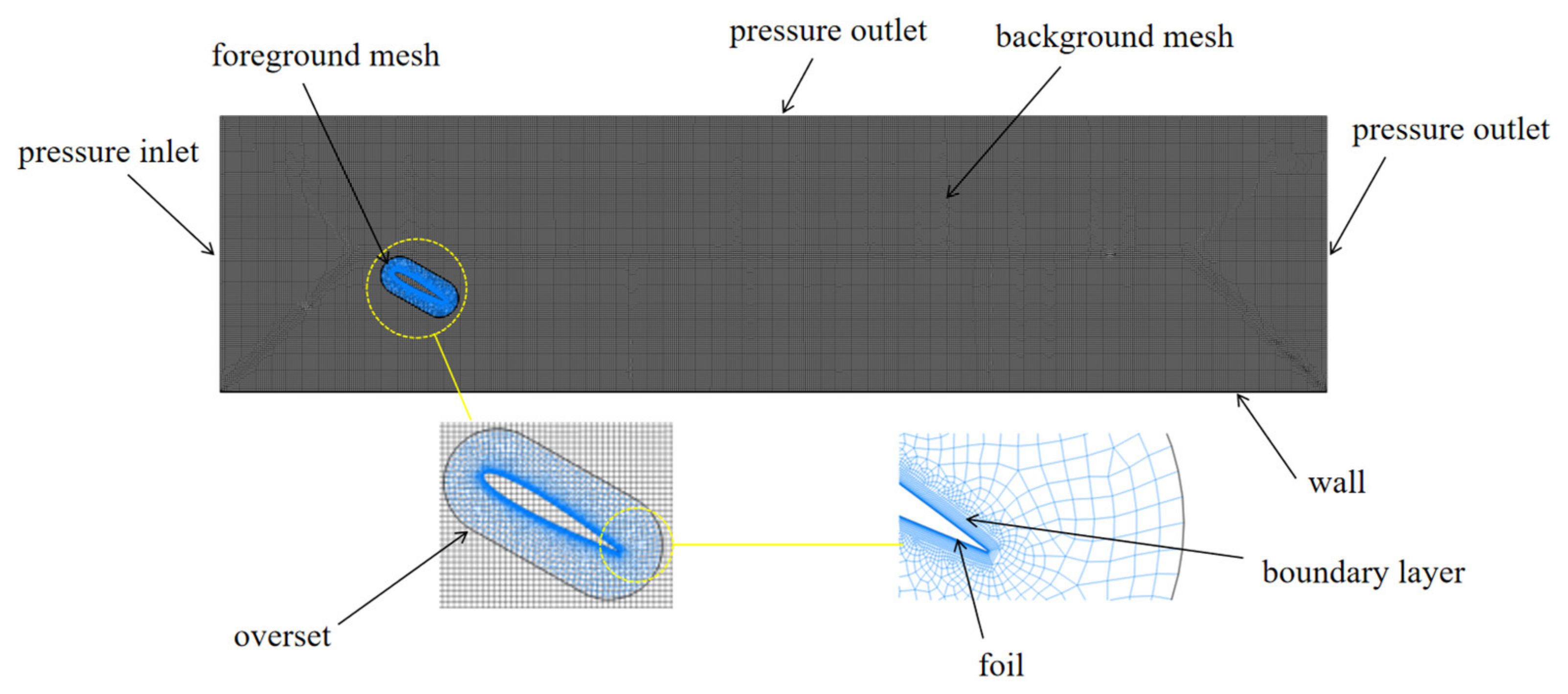
3.3. Mesh Generation and Computational Setup

By reviewing the relevant literature, we understood that the water depth of urban rivers in the southern regions of China is generally within 2 m. For the sake of calculation convenience, in this paper, we set the distance from the free surface to the riverbed at 1.5 m in the numerical simulation. To avoid issues of negative cell volumes during computation, we employed User-Defined Functions (UDFs) and overset grid techniques to model the movement of biomimetic hydrofoils within the flow field. To allow the generated vortices to fully develop, the overall computational domain was set to 6 × 1.5 m. The computational domain included foreground grids representing the moving biomimetic hydrofoils and background grids representing the stationary central cross-section of the river channel.

The meshing method used in this paper is Quadrilateral Dominant. In the numerical calculation process, the overset grid technology was used to first remove the area where the foreground grid overlapped with the background grid, and then data were transferred between adjacent grid cells through interpolation. Therefore, in order to improve the calculation accuracy, we performed mesh refinement around the hydrofoils and at the riverbed to accurately simulate the boundary layer effects and to set the global dimensions of the foreground and background grids to be identical.

We assumed a zero-flow velocity when the biomimetic pump ceased operation; therefore, the river inlet boundary condition was set as the pressure inlet, and the outlet boundary condition was set as the pressure outlet to simulate a stagnant water environment. The surface boundary condition was set as the pressure outlet, the outermost boundary of the foreground grid was set as the overset, and both the biomimetic hydrofoil surfaces and the riverbed were set as no-slip walls, as shown in Figure 4. The movement of the foreground grid, which represents the motion of the biomimetic hydrofoil, was defined by UDFs. The coupled algorithm for pressure–velocity coupling was employed using the first-order upwind scheme for the discretization of the turbulent kinetic energy equation and the turbulence dissipation rate. The momentum equation was discretized using the second-order upwind scheme.

3.4. Grid Independence Verification

In order to maintain high simulation accuracy while minimizing the simulation time, we performed a grid dependency study. The validation conditions were set with an average inlet velocity of $\overline{U}$ = 0.5 m/s; a heave amplitude of A_max = 0.15 m; a pitch amplitude of θ_max = 30°; a motion frequency of ƒ = 1 Hz; a channel depth of 1 m; and an installation height of H = 0.5 m.

We selected four sets of grids—with the total number of cells being 20,000, 40,000, 100,000, and 150,000—for the grid independency verification, as shown in Figure 5. It is evident from the graph that the grids with 20,000 and 40,000 cells exhibit greater errors compared to those with 100,000 and 150,000 cells. To ensure accuracy while minimizing computation time, we chose the 100,000-grid count for subsequent simulation calculations.

3.5. Method Validation

To validate the effectiveness of the simulation method, we compared the simulation data under the same conditions as the experimental data obtained from [25], verifying the effectiveness of the numerical simulation method.

Based on the experimental conditions from [25], a numerical simulation model was established with a computational domain size of 50 c × 12 c; an inlet flow velocity of $\overline{U}$ = 0.4 m/s; a phase difference of φ = −π/2; a pitch motion amplitude of θ_max = 23°; a biomimetic hydrofoil chord length of c = 0.1 m; a heave amplitude of A_max = 0.75 c = 0.075 m; the distance from the pivot axis to the leading edge of the biomimetic hydrofoils at L = 1/3 c = 0.03 m; and an operating frequency of ƒ = 0.8 Hz.

By comparing the thrust and lift of the hydrofoil obtained from the numerical simulation calculations with the experimental data, as shown in Figure 6, we found good consistency between them, which indicates that the numerical simulation method adopted in this paper is effective. The phase error is due to the fact that the inlet flow velocity of the towing tank experiment is passively generated by the hydrofoil drag, and the flow generated by this method has a certain delay error.

4. Results and Discussion

4.1. Effect of Installation Height and Operating Frequency on Maximum Near-Bed Velocity

When the maximum near-bed velocity of the bottom sediment exceeds the critical incipient velocity of the sediment, the sediment can be considered to begin mobilizing. To study the relationship between installation height and operating frequency with maximum near-bed velocity as accurately as possible, while also reducing the time cost required for simulation and facilitating subsequent analysis and discussion, we evenly divided an installation height of 1.5 m into five equal parts using the chord length (c = 0.3 m) as the interval. The use of the hydrofoil chord length as an interval is to improve the applicability of the study results without unduly increasing the computational requirements. However, since the biomimetic pump is beyond its effective working range and cannot operate normally when the installation heights are 0 m and 1.5 m, we chose the middle four installation heights for the simulation. Accordingly, the installation heights set in this study were c = 0.3 m, 2 c = 0.6 m, 3 c = 0.9 m, and 4 c = 1.2 m.

Since the variation in operating frequency has a minimal impact on the pumping performance of the biomimetic pump when the working frequency is low, to ensure the accuracy of conclusions in the low-frequency range while also considering higher-frequency conditions, we set the operating frequencies to 0.5 Hz, 0.8 Hz, 1.4 Hz, 2.3 Hz, 3.5 Hz, and 5 Hz. By focusing on these representative points, rather than employing a comprehensive sweep, we aimed to strike a balance between obtaining meaningful insights into the pump’s behavior and managing the considerable computational demands and time constraints inherent in extensive frequency sweeps. This approach ensures a thorough yet feasible investigation, considering the trade-off between the depth of analysis and practical resource allocation.

A numerical study was conducted for the aforementioned working conditions. The method to obtain the maximum near-bed velocity was as follows. First, a horizontal line was selected at the height of one sediment particle diameter (0.013 mm) above the riverbed [22,23], and the time-averaged value of the flow velocity parallel to the riverbed direction was calculated for each point on this line, from which the maximum value was taken to represent the maximum near-bed velocity. The interest range was between 0.5 m in front of the hydrofoil’s pivot and 5 m. The maximum near-bed velocity data obtained based on the above method are summarized in

Table 2. Maximum near-bed velocities (m/s) corresponding to different installation heights and operating frequencies.

Operating Frequencies (Hz)	Installation Heights (m)
	0.3	0.6	0.9	1.2
0.5	0.028	0.015	0.004	0.040
0.8	0.066	0.036	0.009	0.083
1.4	0.176	0.099	0.026	0.190
2.3	0.408	0.237	0.089	0.479
3.5	0.796	0.487	0.212	0.965
5.0	1.371	0.875	0.399	1.676

.

From the table above, we can see that the maximum near-bed velocity reached its peak value when the installation height was 4 c and the operating frequency was 5 Hz, while the minimum value of the maximum near-bed velocity occurred when the installation height was 3 c and the operating frequency was 0.5 Hz.

To investigate the variation patterns of the maximum near-bed velocity with respect to the operating frequency and installation height, separate plots were created to illustrate the changes in the maximum near-bed velocity with the operating frequency and with the installation height, as shown in Figure 7.

The graph indicates that, at the same installation height, a quadratic function relationship forms between frequency and maximum near-bed velocity. As the frequency increases, the maximum near-bed velocity on the riverbed also increases. Moreover, at the same frequency, as the installation height increases, the maximum near-bed velocity gradually decreases, approximately showing a linear relationship, reaching the minimum value at installation height H = 3 c, after which it begins to increase again.

To investigate the cause of the increase in maximum near-bed velocity, we plotted the vorticity and velocity contour diagrams at different installation heights when the operating frequency is 5 Hz. The vorticity diagram is shown in Figure 8.

The above figure shows the vorticity diagrams during a cycle at different installation heights when the operating frequency is consistently 5 Hz. When the installation height is less than a certain value (i.e., H ≤ 3 c), the biomimetic hydrofoils exert a squeezing effect on the water vortices below as they move downwards. The water vortices deform under the squeezing action of the biomimetic hydrofoils and the riverbed, causing the rotation center of the water vortices to shift forward. As the biomimetic hydrofoils move to their extreme downward position, the counterclockwise-rotating trailing vortices shed off. Since the rotation center of the water vortices below the biomimetic hydrofoils shifted forward when squeezed, the shed trailing vortices descend to the rear of the deformed water vortices’ rotation center under gravity. This causes the vortices rotating in opposite directions to arrange alternately in a horizontal pattern, forming multiple pairs of reverse von Kármán vortex streets. During their movement, the vortices in both directions cancel each other out, and the fluid in the gaps of the vortex street accelerates to form a nearly horizontal jet. When the biomimetic pump exceeds a certain height (i.e., H > 3 c), the biomimetic hydrofoils cannot effectively compress the water vortices below during its downward motion, and the forward shift in the rotation center of the lower vortices is insufficient. This results in the counterclockwise-rotating trailing vortices falling in front of the deformed water vortices’ rotation center after shedding, failing to form multiple pairs of reverse von Kármán vortex streets. At this time, an obliquely downward jet is produced between the water vortices below the hydrofoils and the counterclockwise-rotating trailing vortices generated by the hydrofoils.

The velocity contour diagrams at different installation heights when the operating frequency is 5 Hz are shown in Figure 9.

From the above figure, we can see that, when the installation height is less than a certain value (i.e., H ≤ 3 c), the trailing vortices form multiple pairs of reverse von Kármán vortex streets. The fluid in the gaps of the vortex street is then accelerated to form a nearly horizontal jet, which leads to a flow field distribution that is nearly horizontal, with the flow velocity at the center of the flow field being greater than the velocities on both sides. As the installation height increases, the height of the generated jet also rises and the high-velocity region in the flow field gradually elevates, causing the low-velocity region of the flow field to act upon the riverbed, which results in a gradual decrease in the maximum near-bed velocity. When the biomimetic pump exceeds a certain height (i.e., H > 3 c), an obliquely downward jet is produced between the water vortices below the hydrofoils and the counterclockwise-rotating trailing vortices generated by the hydrofoils. This causes the high-velocity region in the flow field to act obliquely downward on the riverbed, leading to an increase in the maximum near-bed velocity.

4.2. Effect of Installation Height and Operating Frequency on the Location of the Maximum Near-Bed Velocity Point

The location of the maximum near-bed velocity point, i.e., the point most strongly affected by the water body, determines the position of maximum scouring of the sediment.

Table 3. Location of the maximum near-bed velocity points that correspond to different installation heights and operating frequencies (m).

Operating Frequencies (Hz)	Installation Heights (m)
	0.3	0.6	0.9	1.2
0.5	1.085	1.805	4.955	0.905
0.8	1.040	1.805	4.955	0.905
1.4	1.040	1.805	4.955	1.085
2.3	1.040	1.850	2.795	1.130
3.5	1.085	1.850	3.065	1.130
5.0	1.130	1.895	3.110	1.130

lists the numerical simulation results of the location of the maximum near-bed velocity point that corresponds to different installation heights and operating frequencies. Here, the location of the maximum near-bed velocity point is defined as the horizontal position on a horizontal line near the bottom where the maximum near-bed velocity occurs. This refers to the horizontal distance from the point of maximum time-averaged value of the flow velocity over a cycle at the riverbed bottom to the hydrofoil’s pivot, where the horizontal distance is measured in the x₁ direction.

From the table above, we can see that the location of the maximum near-bed velocity point reaches its maximum when the installation height is 3 c and the operating frequency is f = 0.5 Hz, at which point the maximum scouring position of the sediment is farthest from the biomimetic pump. Conversely, the location of the maximum near-bed velocity point attains its minimum when the installation height is 4 c and the operating frequency is f = 0.5 Hz; at this point, the maximum scouring position of the sediment is closest to the biomimetic pump.

To analyze the pattern of variation in the maximum near-bed velocity point, diagrams of the location of the maximum near-bed velocity point with respect to the changes in operating frequency and installation height were plotted, as shown in Figure 10.

From the figure above, we can observe that, when the installation heights are c, 2 c, and 4 c, the location of the maximum near-bed velocity point remains essentially unchanged with varying operating frequencies. However, when the installation height is 3 c, as the operating frequency increases, the distance between the maximum near-bed velocity point and the biomimetic pump rapidly decreases from its farthest point and then remains largely constant with further increases in operating frequency. Figure 10b shows that, when the operating frequency is held constant, the distance between the maximum near-bed velocity point and the biomimetic pump significantly increases with rising installation height, reaching a maximum at an installation height of 3 c, after which it gradually decreases.

Since the position of the maximum near-bed velocity point experiences a sudden change when the operating frequency increases from 1.4 Hz to 2.3 Hz with the biomimetic pump installed at a height of 3 c, to investigate the cause of this rapid change in the position of the maximum near-bed velocity point with frequency, time-averaged velocity curves at different near-bed locations for frequencies of 1.4 Hz and 2.3 Hz were plotted, as shown in Figure 11.

From the figure above, we can see that, when the operating frequency is 1.4 Hz, as the horizontal position gradually increases, the maximum near-bed velocity first decreases and then increases, eventually reaching its maximum at the farthest point from the biomimetic pump. When the operating frequency is 2.3 Hz, with the gradual increase in horizontal position, the maximum near-bed velocity slightly decreases before rapidly increasing to reach its maximum value and then gradually decreases again; at this point, the location of the maximum near-bed velocity is no longer the farthest from the biomimetic pump.

To further analyze the causes of this result, vorticity diagrams and velocity contour plots were created for an installation height of 3 c at operating frequencies of 1.4 Hz and 2.3 Hz, as shown in Figure 12 and Figure 13.

Figure 12 shows the vorticity diagram when the installation height is 3 c. From the figure, we can see that, when the operating frequency is 1.4 Hz, the trailing vortices generated by the biomimetic hydrofoils are relatively weak. As the vortices move in the direction of the water flow, the opposite vortices dissipate quickly. The jet produced by the reverse von Kármán vortex street is also weak at this time. This is reflected in Figure 13’s velocity contour plot, where the high-velocity area of the flow field is too small, covering a large area of the riverbed with low-velocity regions. Only the farthest point near the riverbed is close to the high-velocity area of the flow field, resulting in the maximum near-bed velocity point being at the farthest location. When the operating frequency increases to 2.3 Hz, the strength of the trailing vortices generated by the biomimetic hydrofoils becomes stronger, and the dissipation of the opposite vortices slows down. The jet produced by the reverse von Kármán vortex street becomes stronger, and the high-velocity region of the flow field expands. This causes part of the high-velocity area to act on the riverbed earlier than the farthest point, resulting in a leftward shift in the maximum near-bed velocity point.

Regarding the reason why the distance between the maximum near-bed velocity point and the biomimetic pump first increases and then decreases with the increase in height, Figure 9 shows that, when the operating frequency is constant and the installation height is less than a certain value (i.e., H ≤ 3 c), as the installation height increases, the high-velocity region of the flow field also gradually rises. This causes the initial contact position of the high-velocity region of the flow field with the riverbed to gradually shift to the right, resulting in a rightward movement of the maximum near-bed velocity point. When the biomimetic pump exceeds a certain height (i.e., H > 3 c), at this time, an obliquely downward jet is generated between the water vortices below the hydrofoils and the counterclockwise-direction trailing vortices. The high-velocity region of the flow field produced by this jet acts directly obliquely downward on the riverbed, causing the maximum near-bed velocity point to rapidly move to the left.

4.3. Threshold Frequency for Sediment Incipient Motion at Specific Installation Heights

In the preceding text, we have calculated that the critical incipient velocity for sediment movement is 13.78 cm/s. This means that, when the time-averaged value of the flow velocity at a point near the riverbed exceeds this value, we can consider that the sediment at the bottom begins to move. To facilitate the rapid calculation of the threshold frequency that causes sediment movement corresponding to the installation height of the bionic pump in practical applications using interpolation methods. In this section, we calculate the threshold frequencies for sediment incipient motion at specific installation heights (integer multiples of chord length).

Polynomial fitting was performed on the data in Figure 7a to obtain the expressions for frequency–maximum near-bed velocity at different installation heights, as shown in

Table 4. Relationship between motion frequency and maximum near-bed velocity.

Installation Height	Polynomial Formula
0.3 m	$\overline{\mu }=0.031x^2+0.1313x-0.0557$
0.6 m	$\overline{\mu }=0.0242x^2+0.0598x-0.026$
0.9 m	$\overline{\mu }=0.0142x^2+0.0113x-0.0097$
1.2 m	$\overline{\mu }=0.0424x^2+0.136x-0.0544$

.

By substituting ${\overline{u}}_{\max }=0.1378 \mathrm{m}/s$ into the above formulas, the threshold frequencies for sediment incipient motion at various heights are obtained, as shown in

Table 5. Threshold frequencies for sediment incipient motion at special installation heights.

Installation Height	Threshold Frequencies
0.3 m	1.15 Hz
0.6 m	1.64 Hz
0.9 m	2.85 Hz
1.2 m	1.06 Hz

.

From the table above, we can conclude that the threshold frequencies for sediment incipient motion when the installation heights are at c, 2 c, 3 c, and 4 c are 1.15 Hz, 1.64 Hz, 2.85 Hz, and 1.06 Hz, respectively.

5. Conclusions

(1)

Changing the installation height and operating frequency of the biomimetic pump can significantly affect the maximum near-bed velocity, thereby impacting the sediment at the bottom. Through numerical simulation, this paper concludes that the minimum value of the maximum near-bed velocity is reached when the biomimetic pump is installed at a height of 3 c and an operating frequency of 0.5 Hz. Conversely, the maximum value is achieved at an installation height of 4 c and an operating frequency of 5 Hz. When the installation height of the biomimetic pump remains constant, as the operating frequency increases, the maximum near-bed velocity also correspondingly increases, following a quadratic function relationship. When the frequency remains constant and the installation height gradually increases, with the height less than or equal to 3 c, the maximum near-bed velocity gradually decreases, reducing the impact of the water on the sediment, reaching the minimum impact at 3 c. However, when the installation height exceeds 3 c, the maximum near-bed velocity begins to increase again, even surpassing the maximum near-bed velocity at the lowest installation height, thereby increasing the impact of the water on the sediment once more;

(2)

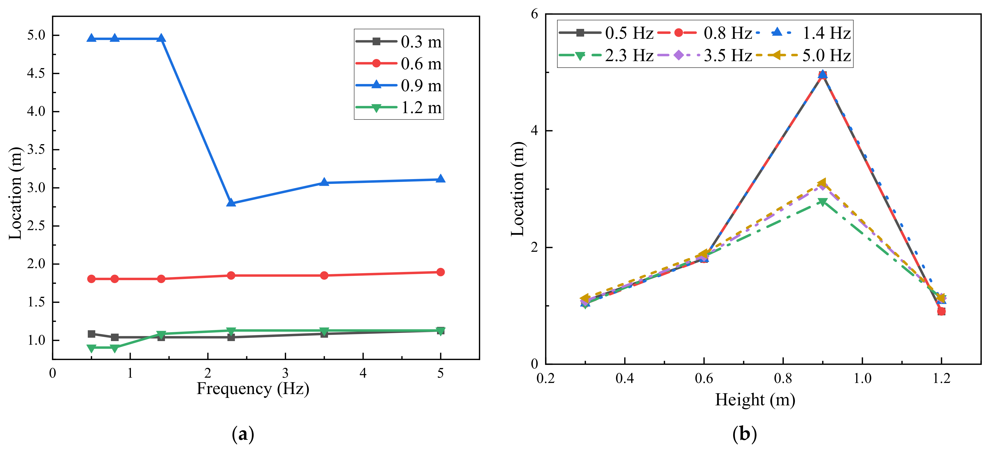
The location of the maximum near-bed velocity point corresponds to the position at which maximum erosion of the sediment occurs. Through numerical simulation, this paper finds that the position where the maximum erosion of the sediment is farthest from the biomimetic pump occurs when the installation height is 3 c and the operating frequency is 0.5 Hz. Conversely, it is closest to the biomimetic pump when the installation height is 4 c and the operating frequency is 0.5 Hz. When the installation height remains constant at c, 2 c, or 4 c, the position where maximum erosion of the sediment does not change significantly with varying operating frequencies. However, when the installation height is 3 c, as the operating frequency increases, the distance between the position where maximum erosion of the sediment and the biomimetic pump rapidly decreases from the farthest point, eventually stabilizing with further increases in operating frequency. When the operating frequency is constant, as the installation height increases, the distance between the position where maximum erosion of the sediment and the biomimetic pump significantly increases, reaching a maximum at an installation height of 3 c, and then gradually decreases;

(3)

To facilitate the rapid approximation of the required biomimetic pump parameters through interpolation and to reduce the complexity of parameter calculation, we obtained the threshold frequencies for sediment incipient motion at installation heights of c, 2 c, 3 c, and 4 c through numerical simulations as 1.15 Hz, 1.64 Hz, 2.85 Hz, and 1.06 Hz, respectively.

References

1. Luo, D.L.; Lu, P.D.; Yu, G.H. Study on the activity of the contaminative water and the impact on the water pollution of change in urban river-net in the east plain region of China. Environ. Eng. 2011, 29, 59–62. [Google Scholar]
2. Phillips, J.D.; Slattery, M.C. Downstream trends in discharge, slope, and stream power in a lower coastal plain river. J. Hydrol. 2007, 334, 290–303. [Google Scholar] [CrossRef]
3. Hongzhe, P.; Chunyan, T.; Acharya, K.; Jian, Z.; Jian, Z.; Ya, Z.; Yixin, C.; Yue, C.; Shan, Y.; Zhenwu, Y. Evaluation of the effect of water diversion on improving water environment in plain river network under the multi-objective optimization. J. Lake Sci. 2021, 33, 1138–1152. [Google Scholar] [CrossRef]
4. Zheng, Y.; Chen, Y.j.; Zhang, R.; Ge, X.F.; Sun, A. Analysis on Unsteady Stall Flow Characteristics of Axial-flow Pump. Trans. Chin. Soc. Agric. Mach. 2017, 48, 127–135. [Google Scholar]
5. Xu, H.; Gong, Y.; Cao, C.J.; Chen, H.X.; Kan, K.; Feng, J.G. 3D Start-up Transition Process of Full Flow System for Shaft-extention Tubular Pump Station. Trans. Chin. Soc. Agric. Mach. 2021, 52, 143–151. [Google Scholar]
6. Hua, E.T.; Zhu, W.; Xie, R.; Su, Z.; Luo, H.; Qiu, L. Comparative Analysis of the Hydrodynamic Performance of Arc and Linear Flapping Hydrofoils. Processes 2023, 11, 1579. [Google Scholar] [CrossRef]
7. Hua, E.T.; Luo, H.T.; Xie, R.; Chen, W.; Tang, S.; Jin, D. Investigation on the Influence of Flow Passage Structure on the Performance of Bionic Pumps. Processes 2022, 10, 2569. [Google Scholar] [CrossRef]
8. Lin, T.; Xia, W.; Pecora, R.; Wang, K.; Hu, S. Performance improvement of flapping propulsions from spanwise bending on a low-aspect-ratio foil. Ocean Eng. 2023, 284, 115305. [Google Scholar] [CrossRef]
9. Du, X.X.; Zhang, Z.D. Numerical analysis of influence of four flapping modes on propulsion performance of underwater flapping foils. Eng. Mech. 2018, 35, 249–256. [Google Scholar]
10. Ding, H.; Song, B.W.; Tian, W.L. Exploring Propulsion Performance Analysis of Bionic Flapping Hydrofoil. J. Northwestern Polytech. Univ. 2013, 31, 150–156. [Google Scholar]
11. Li, G.Z.; Chang, X.; Deng, N.Y.; Yu, P.Y. Research on the propulsive performance of the non-sinusoidal plunging in-line tandem hydrofoils. Ship Sci. Technol. 2022, 44, 94–100. [Google Scholar]
12. Hua, E.T.; Su, Z.X.; Xie, R.S.; Chen, W.Q.; Tang, S.W.; Luo, H.T. Optimization and experimental verification of pivot position of flapping hydrofoil. J. Hydroelectr. Eng. 2023, 42, 128–138. [Google Scholar]
13. Hua, E.T.; Chen, W.Q.; Tang, S.W.; Xie, R.S.; Guo, X.M.; Xu, G.H. Water Pushing Flow Characteristics of Flapping Hydrofoil Device in Small River. Trans. Chin. Soc. Agric. Mach. 2022, 53, 154–162. [Google Scholar]
14. Li, F.; Yu, P.; Deng, N.; Li, G.; Wu, X. Numerical analysis of the effect of the non-sinusoidal trajectories on the propulsive performance of a bionic hydrofoil. J. Appl. Fluid Mech. 2022, 15, 917–925. [Google Scholar]
15. Zhou, J.; Yan, W.; Mei, L.; Shi, W. Performance of Semi-Active Flapping Hydrofoil with Arc Trajectory. Water 2023, 15, 269. [Google Scholar] [CrossRef]
16. Mei, L.; Zhou, J.; Yu, D.; Shi, W.; Pan, X.; Li, M. Parametric analysis for underwater flapping foil propulsor. Water 2021, 13, 2103. [Google Scholar] [CrossRef]
17. Yang, J.Q.; Tang, L.M.; Huang, P.; Sun, J. Study on incipient velocity of fine sediment in Yongiiang River Estuary. Water Resour. Hydropower Eng. 2018, 49, 149–154. [Google Scholar]
18. Zhou, S.F.; Huang, Z.W.; Wang, Z.C. Experimental study on initiation law of consolidated cohesive sediment in Poyang Lake. J. Hohai Univ. (Nat. Sci.) 2023, 51, 99–104. [Google Scholar]
19. Sun, Z.L.; Zhang, C.C.; Huang, S.H.; Liang, X. Scour of cohesive nonuniform sediment. J. Sediment Res. 2011, 3, 44–48. [Google Scholar]
20. Xiao, H.; Cao, Z.D.; Zhao, Q.; Han, H.S. Experimental study on incipient motion of coherent silt under wave and flow action. J. Sediment Res. 2009, 3, 75–80. [Google Scholar]
21. Shaheed, R.; Mohammadian, A.; Kheirkhah, G.H. A comparison of standard k–ε and realizable k–ε turbulence models in curved and confluent channels. Environ. Fluid Mech. 2019, 19, 543–568. [Google Scholar] [CrossRef]
22. Wu, Z.S.; Zhang, G.G.; Kou, T.; Gao, Y.; Li, L.L. Research on Sediment Incipient Velocity Based on Probability Statistics Theory. J. Chang. River Sci. Res. Inst. 2017, 34, 7–11. [Google Scholar]
23. Zhong, X.Y.; Wang, C.H.; Yu, C.R.; Wen, L.; Duan, P.Y. Characteristics of sediments and nutrient release under different flow velocity. Acta Sci. Circumstantiae 2017, 37, 2862–2869. [Google Scholar]
24. Ma, Z.P.; Zhang, G.G.; Gao, G.Y.; Tian, G.Z. Discussion on incipient condition of a noncohesive sediment particle on slope under 3D flow. J. Sediment Res. 2014, 39, 36–41. [Google Scholar]
25. Schouveiler, L.; Hover, F.S.; Triantafyllou, M.S. Performance of flapping foil propulsion. J. Fluids Struct. 2005, 20, 949–959. [Google Scholar] [CrossRef]
Figure 1. Schematic diagram of the structure of NACA0012 airfoils.
Water 16 01925 g001
Figure 2. Biomimetic pump installation height diagram.
Water 16 01925 g002
Figure 3. Schematic of a biomimetic hydrofoil motion, where Amax = 0.5 c denotes the amplitude of the heaving motion of the biomimetic hydrofoil; θmax = π/6 represents the amplitude of the pitching motion; and T is the period of the motion.
Water 16 01925 g003
Figure 4. Boundary condition diagram.
Water 16 01925 g004
Figure 5. Grid independence verification.
Water 16 01925 g005
Figure 6. Comparison between numerical results and experimental data: (a) thrust variation curve; (b) lift variation curve.
Water 16 01925 g006
Figure 7. Variation in maximum near-bed velocity with installation height and operating frequency: (a) variation with operating frequency; (b) variation with installation height.
Water 16 01925 g007
Figure 8. Vorticity contour diagrams over one cycle at different installation heights when the operating frequency is 5 Hz: (a) H = c; (b) H = 2 c; (c) H = 3 c; (d) H = 4 c.
Water 16 01925 g008aWater 16 01925 g008b
Figure 9. Velocity contour diagrams at different installation heights when the operating frequency is 5 Hz: (a) H = c; (b) H = 2 c; (c) H = 3 c; (d) H = 4 c.
Water 16 01925 g009aWater 16 01925 g009b
Figure 10. Variation in the location of the maximum near-bed velocity point with installation height and operating frequency: (a) variation with operating frequency; (b) variation with installation height.
Water 16 01925 g010
Figure 11. Time-averaged velocity curves at different near-bed locations for frequencies of 1.4 Hz and 2.3 Hz.
Water 16 01925 g011
Figure 12. Vorticity diagram for an installation height of 3 c at operating frequencies of 1.4 Hz and 2.3 Hz: (a) f = 1.4 Hz; (b) f = 2.3 Hz.
Water 16 01925 g012aWater 16 01925 g012b
Figure 13. Velocity contour plots for an installation height of 3 c at operating frequencies of 1.4 Hz and 2.3 Hz: (a) f = 1.4 Hz; (b) f = 2.3 Hz.
Water 16 01925 g013