Abstract
Saudi Arabia is threatened by recurrent flash floods caused by extreme precipitation events. To mitigate the risks associated with these natural disasters, we implemented an advanced nationwide flash flood forecast system, boosting disaster preparedness and response. A noteworthy feature of this system is its national-scale operational approach, providing comprehensive coverage across the entire country. Using cutting-edge technology, the setup incorporates a state-of-the-art, three-component system that couples an atmospheric model with hydrological and hydrodynamic models to enable the prediction of precipitation patterns and their potential impacts on local communities. This paper showcases the system’s effectiveness during an extreme precipitation event that struck Jeddah on 24 November 2022. The event, recorded as the heaviest rainfall in the region’s history, led to widespread flash floods, highlighting the critical need for accurate and timely forecasting. The flash flood forecast system proved to be an effective tool, enabling authorities to issue warnings well before the flooding, allowing residents to take precautionary measures, and allowing emergency responders to mobilize resources effectively.
Keywords:
flash flood; Saudi Arabia; flood forecasting; flood warnings; WRF; hydrologic model; hydraulic model 1. Introduction
Floods are among the most frequent and dangerous natural disasters globally, and their impacts are likely to increase as climate change progresses and the population grows [1,2,3,4], regardless of location, climate, or level of development of the affected country [5,6,7]. Flash floods, in particular, have escalated drastically due to climate change and ongoing urbanization [8,9], with disasters reported worldwide.
The effect of climate change is just one factor contributing to the rising impacts of floods [10]. A combination of societal factors [11] and methodological limitations in modeling and forecasting make cities more vulnerable to flooding, especially in arid environments [12,13,14].
Flash flood forecasting is challenging [12] and is made more so by some features that distinguish it from riverine flood forecasting and add to its uncertainty [6,15,16]. Flash floods are driven mainly by convective precipitation events, with high spatiotemporal variability limiting their predictability [15,17], also because of the inherently three-dimensional and turbulent nature of the atmosphere [18]. Furthermore, flash floods are characterized by fast dynamics and high specific discharges [15,19], which require high-resolution models to be captured efficiently. Bannister et al. [20] provided a review of some of the most significant challenges in predicting convective events driving flash floods, including the needs for large volume of water-related observations (e.g., from radar, microwave, and infrared instruments), the necessity to analyze hydrometeors of various nature at multiple scales [21], the growing importance of local-forecast errors due to the scale at which these events happen, the requirement to account for the flow-dependent multivariate balance between atmospheric water and both dynamical and mass fields [18], and the inherently non-Gaussian nature of atmospheric water variables [20]. This complexity is further heightened by the fact that convective storms are influenced by local topography, land use, and surface conditions, which can vary widely and affect storm development [20].
Although some countries offer operational flash flood monitoring services based on weather radar rainfall estimates [22,23,24], the lag time between a rainfall burst and flood impact is too short to grant a meaningful period of anticipation in affected domains [12,25]. The importance of providing accurate inundation forecasts at the scale of specific critical locations within a broad region underscores the need for increased anticipation and finer flood impact modeling than that on which current operational forecasts are based. Indeed, flash flood impacts occur at the scale of individual properties, and accurate warning needs to account for the specific processes of the urban environment, where stormwater follows multiple flow paths and interacts with artificial structures [26]. In addition, near-real-time inundation forecasts may require performing ensembles of simulations with a latency of just a few minutes [27] and a forecast horizon short enough to be significant but large enough to grant time for preparedness.
Simulating the discharge and accurately determining inundation are also challenging for large-scale applications. Most rainfall-runoff models operate on spatial scales on the order of 1 km. Still, the high number of calibration parameters may become a constraint because the systematic observational data are generally missing. The scale at which flash floods develop is too small for conventional rain or discharge measurement gauges to sample them effectively [28]. Moreover, flash floods are relatively rare at the local scale, with flood impacts varying in location, especially in urban environments, making it hard to collect inundation references. Even from a modeling perspective, solving a bidimensional inundation tends to become too computationally expensive for implementation in operational systems.
Nowadays, however, new numerical methods, the deployment of high-performance computing [29,30,31,32], and new and highly detailed datasets often derived from remote sensing [33,34,35] are offering new opportunities to improve the models’ accuracy and make them sufficiently reliable to enhance our understanding of the generation mechanisms of flash floods.
Although Saudi Arabia is in a region characterized as arid/semi-arid [36], flash floods are quite frequent there, and they are becoming increasingly so [37,38,39,40,41,42,43]. The events often cause heavy human casualties, as well as significant damage to infrastructure, even though the country lacks permanent year-round rivers.
The Arabian Peninsula (AP) features a diverse climatic range, with higher temperatures and inconsistent rainfall patterns [44,45], with areas mostly characterized by winter snow precipitation in the Asir Province to those featuring intense humidity around the Arabian Gulf and parts characterized by extreme heat, such as the Rub Al Khali desert, or monsoon-dominated climate in the Qara Mountains of Dhofar [45]. Rainfalls are characterized mostly by irregular, heavy rainstorms, on only a few days in a year and only in some areas, with the southwestern area being mostly controlled by orography and showing local convective precipitation [46,47]. Various authors highlighted shifts in temperature and evaporation rates [48] and precipitation intensity [48,49,50,51], resulting in more impactful and frequent flooding. Historical analysis showcased an average increase in precipitation intensity of about 15 to 20% in some areas, such as Jeddah [49], with rising trends in daily maximum precipitation, suggesting an increasing flood risk [52] across AP overall [44,50].
Flooding impacts due to these changes in climate drivers are further exacerbated by rapid population growth, urbanization, and transformation of large areas of sandy desert into concrete-built impervious surfaces that delay rainwater infiltration [53] and affect the natural drainage [52,53,54,55,56,57,58]. Flash floodwaters travel at high speed without a predetermined path and carry a high debris load [59]. Accumulated debris within drainage conduits in urban areas and in minor ephemeral wadis originating from previous runoff events, furthermore, can locally increase the flood potential [60]. Risk further increases due to the fact that many urban settlements and other infrastructure developments were built over the years on dry wadi beds during a long time of aridity [56,57,61,62].
The nature of these flows demands a warning system that can provide ample lead time and local-scale modeling. However, the generally limited availability of data records and field observations poses unique challenges to researchers and practitioners.
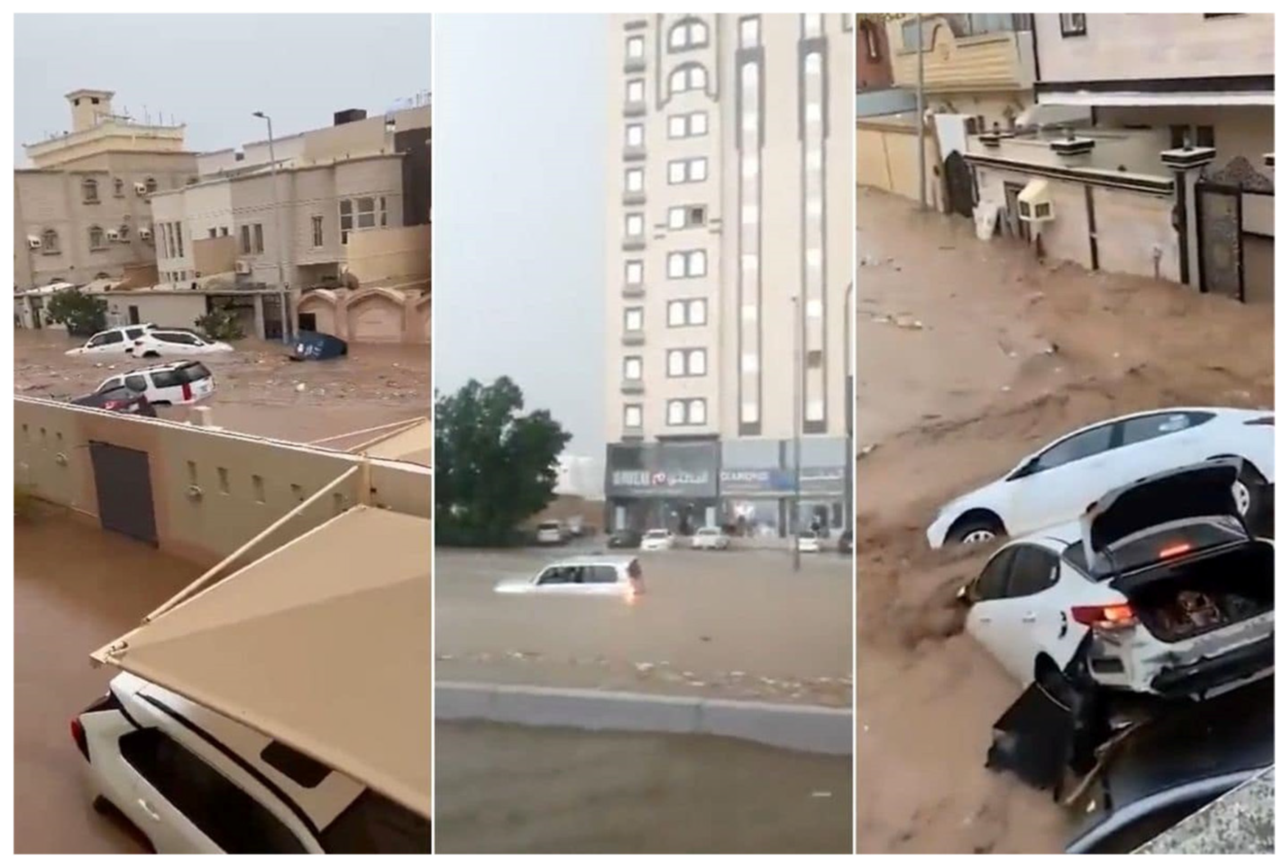
This paper introduces the Flash Flood Forecasting System of the National Center for Meteorology of the Kingdom of Saudi Arabia. In collaboration with Saudi Business Machines, LENOVO Super-Computers, the University of Connecticut, Weather & Marine Engineering Technologies, and the University of Athens, the Center implemented a first-of-its-kind operational instance of a flash flood forecast system over the Arabian Peninsula. As the rapid onset of flash flood events hinders mitigation measures and limits timely decisions that could save lives and avert property losses, the principal objective of the current study was to investigate the predictive capability of the operational tool during a flash flood that struck in western parts of Saudi Arabia after torrential rain on 24 November 2022 (Figure 1). During this event, the city of Jeddah in Makkah Province recorded 179 mm of rain in six hours, the heaviest ever recorded in the area. The result was widespread flash floods across the urban and rural areas of Jeddah, with floodwaters inundating numerous streets and closing major routes, including the main highway between Jeddah and Makkah. In the aftermath, power outages and water supply issues were also reported in parts of the city. In the following sections, we describe the forecasting system and models, validate the precipitation, hydrological, and flood inundation forecasts, and discuss the forecast system’s performance for 24 November 2022. We close with recommendations for future system development.

Figure 1.
Jeddah flood, images from videos available online.
2. Materials and Methods
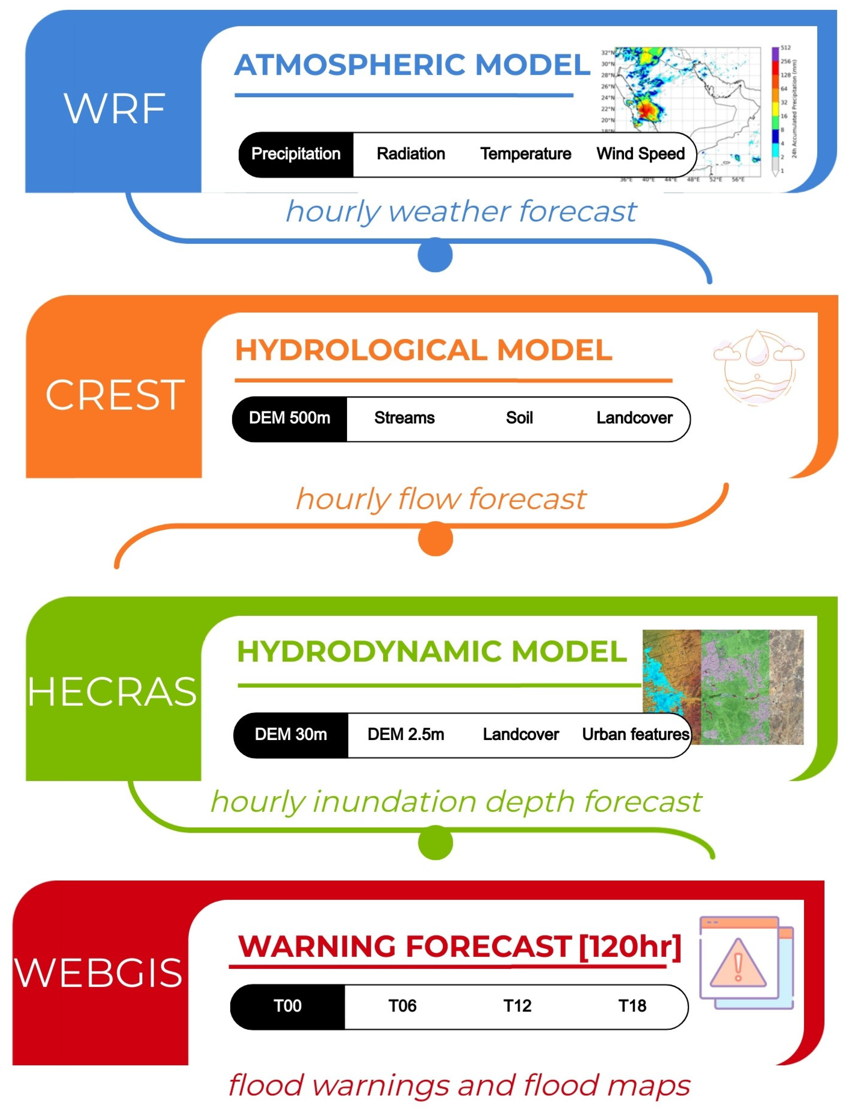
The National Center for Meteorology (NCM) Flash Flood Forecasting System integrates numerical weather forecasts from the Weather Research and Forecasting (WRF) model [63] with the Coupled Routing and Excess STorage (CREST [64] and a 2D hydrodynamic model (HEC-RAS; see Figure 2). The atmospheric component runs at cloud-resolving scales (1.6 km) to incorporate local features and strong convection. The hydrological and hydrodynamic models run at variable spatiotemporal resolution: rainfall-runoff generation and routing are both at 500 m-by-hourly, and floodplain dynamics are at 30 m-by-hourly and 2.5 m-by-hourly. The significant computational requirements dictate the domain differences, with CREST running over large natural basins, while HEC-RAS runs over small basins with dense infrastructure and high exposure to floods. The Flood Forecasting System runs over multiple nested domains that are operationally selected based on the amount of exposure—based on the presence of human beings and their livelihoods, assets, infrastructure, and resources in places where flood hazards could occur. Each domain runs using different cores, depending on the size of the domains. The system takes about 1 to 2 h to produce results, and it is triggered every 6 h, with a forecast window of 120 h (5 days).
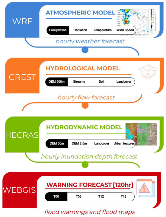
Figure 2.
Overview of the NCM Flash Flood Forecasting System. The system combines the WRF weather model, the CREST hydrological model, and the HEC-RAS 2D hydraulic model. WRF hourly weather forecasts force CREST to generate hourly discharge time series four times daily. Finally, the hydrographs derived from the hydrological model serve as input hydrographs in the 2D HEC-RAS hydrodynamic model for flood inundation modeling and mapping.
The following sections describe the domains and setups for the atmospheric, hydrological, and hydrodynamic models.
2.1. Atmospheric Model Domain and Setup
During the past decade, high-resolution and convection-permitting numerical weather prediction (NWP) models have improved weather forecasting systems to the point where they can capture heavy precipitation events [65]. Among the many existing NWP operational and research applications, WRF is the most popular atmospheric model used [66]. This popularity is attributed to its ability to employ a wide range of physical parameterizations (such as microphysics, convection, planetary boundary layer, radiation, and surface physics), its capability to run at fine scales, and its support from a large and active user community. Furthermore, the continuous development and enhancement of WRF, along with its proven scalability and reliable output, contribute to its widespread adoption.
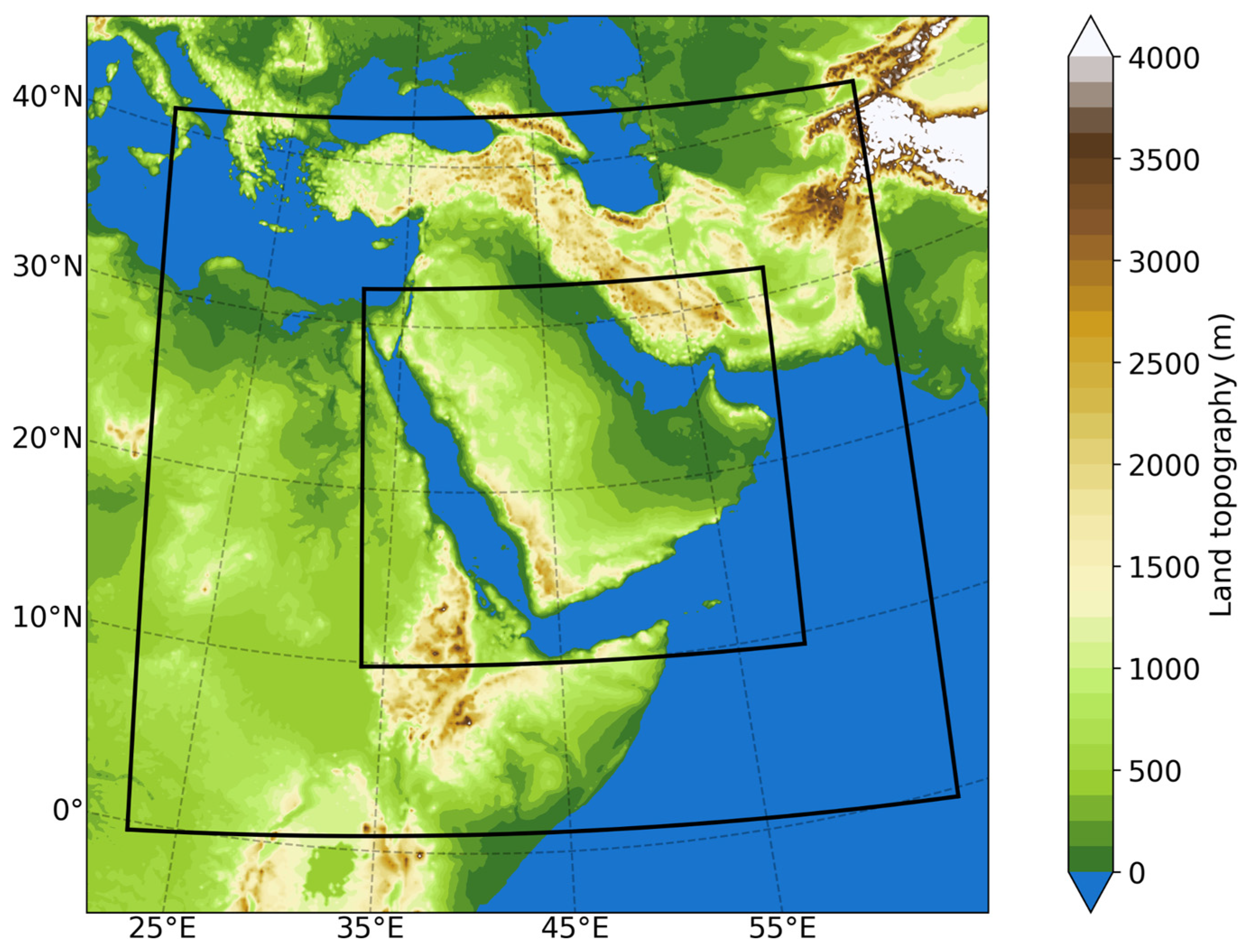
For the NCM operational system, WRF runs in two-way nesting interactive nests (Figure 3). The nests are used to enhance regional weather simulations by increasing spatial resolution in specific areas. This improves the representation of localized phenomena (e.g., thunderstorms, complex terrain effects) and overall forecast accuracy, providing computational efficiency by focusing resources where high resolution is most needed.
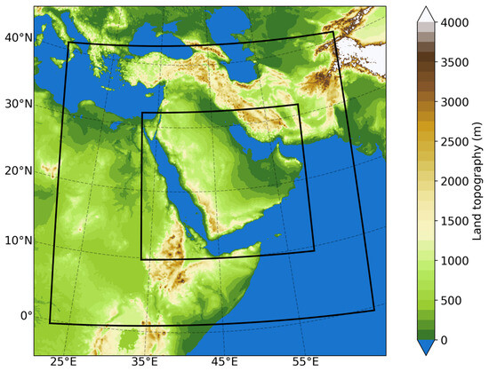
Figure 3.
WRF model domain: black boxes highlight the coarse nest, including parts of Africa, Asia, and Europe, with a spatial resolution of 4.8 km, and the fine nest, covering the Arabian Peninsula with a spatial resolution of 1.6 km.
The coarse nest covers a large domain, including parts of Africa, Asia, and Europe, with a spatial resolution of 4.8 km, while the fine nest covers the Arabian Peninsula with a spatial resolution of 1.6 km (Figure 3). We apply a level-division scheme with 48 vertical levels. The model setup and the resolutions employed were chosen to balance computational efficiency with the need for detailed forecasts. The 4.8 km resolution is used to capture larger-scale atmospheric processes and to provide a comprehensive overview of a wider region. At the same time, the 1.6 km resolution is employed to capture finer-scale atmospheric features, such as convective processes (explicitly), which are critical for accurately forecasting heavy precipitation events. The available resources allow this model setup to operate in four daily cycles (00 UTC, 06 UTC, 12 UTC, 18 UTC), with the outer domain configured to provide a 10-day forecast and the inner one a 5-day forecast (+12 h spin-up time). The model’s predictability depends on many factors, such as initial and boundary conditions, physics parameterization, etc. When focusing on forecasting strong and localized convective activity, the best forecast is expected within a 24-h window. Beyond this period, the forecasting capabilities gradually decline, affecting both the spatiotemporal distribution and intensity of the event. Patlakas et al. (2023) [67] provided more information regarding the configuration and performance of the modeling system.
2.2. The Hydrological and Hydrodynamic Model Domain and Setup (CREST-HEC2D)
Figure 4 shows the settings for the integrated CREST-HEC2D system for the whole domain and for the area affected by the November 2022 event.
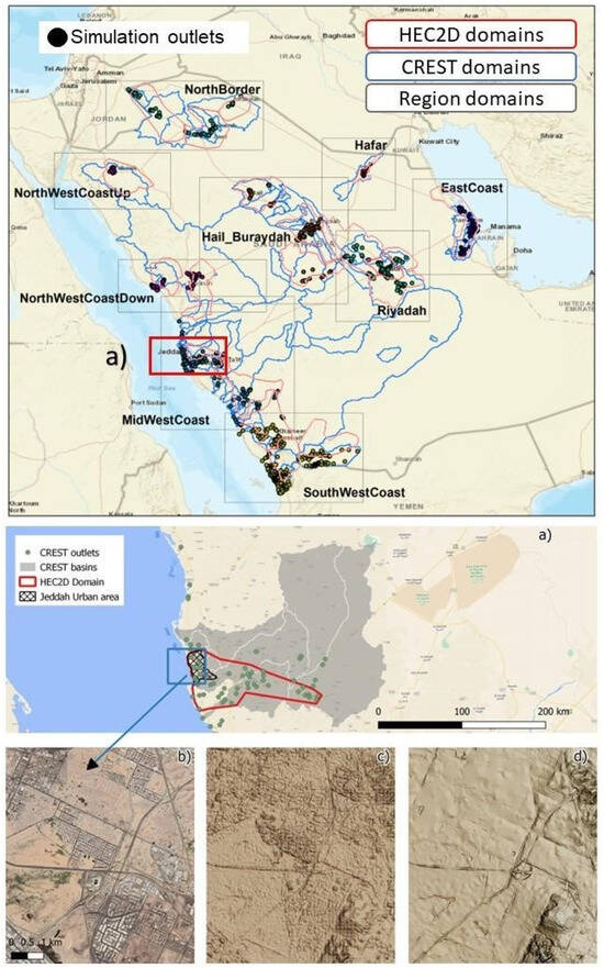
Figure 4.
CREST-HEC2D settings for the whole system, with a zoom to the midwest coast (red square in the map at the top and highlighted in panel (a) below that). Panel (a) compares the CREST watersheds and their outlets to the HEC2D domain for the 24 November 2022 event. The midwest coast domain encompasses the cities of Jeddah, Makkah, and Taif. The bottom images display a detailed view of an area in Jeddah (panel (b)), with the corresponding terrain at 30 m (panel (c)) and the high-resolution terrain at 2.5 m (panel (d)). The quality and resolution of the terrain allow the depiction of the footprints of buildings and roads, as highlighted by the roughness of the map in panel (c). High resolution (panel (d)) provides detailed information for improved flood modeling.
CREST is a distributed hydrological model that integrates precipitation-runoff and channel routing processes at high spatiotemporal resolution (30 m–1 km/hourly), fitting most land cover types. The model is currently applied for real-time flood forecasting and historical analysis over selected locations in Connecticut, USA [64,68,69]. For the operational Flash Flood Forecast System, the model considers land cover information (“MOD12Q1”) retrieved from the Moderate Resolution Imaging Spectroradiometer (MODIS; [70] and integrates precipitation-runoff and channel routing processes to produce discharge at hourly timesteps based on the input climatic forcing from the atmospheric module described above. The rainfall-runoff module runs at 500 m resolution, following the input variable of the finest resolution (in this case, MOD12Q1). The direct runoff is then downscaled to the Copernicus 30m GLO-30m digital elevation model (DEM) grids [71] for routing.
We produced flood inundation characteristics using HEC-RAS 5.0.7 for Linux. The implemented system takes full advantage of a standard calibration model for each domain that is automatically updated based on input streamflow data. To perform such automation, we developed a coupling algorithm in Python to provide a set of computational subroutines that allows complete automation of the HEC-RAS model, from preparing the input flow conditions to simulating the event and gathering the results into meaningful maps. This automation reduces the need for excessive manipulation of files and manual adjustments in the model itself, which presents a significant advantage when essential decisions must be made relatively quickly.
The control of HEC-RAS computations involves three main components:
1. Data Retrieval Functionality (DRF). This component retrieves the input flow data and synchronizes with CREST’s completion of its runs. After each run, the data retrieval packet is triggered independently for each domain. It collects results for each outlet, assigns flows to boundary conditions in HEC-RAS, and sets unsteady flow rates. This process embeds the simulation’s start and end time, along with flow data, into the HECRAS input files.
2. Operation Functionality (OF). The OF is responsible for managing operations such as opening, closing, and running HEC-RAS. It performs the unsteady flow simulation in three steps: reading data from the modified input plan file, executing the RasUnsteady.exe program, which reads hydraulic properties tables from the pre-processor, along with boundary conditions and flow data, and finally, conducting the unsteady flow calculations.
3. Post-Processing Functionality (PostProc). PostProc handles the production of results and the web display. Since HEC-RAS 5.0.7 for Linux does not directly provide inundation maps at the resolution of the input DEM (Digital Elevation Model), the post-processing functionality retrieves inundation depth at the computational cell level, interpolates it to the DEM resolution using common Python 3.10 packages (numpy and scipy), and generates the final 2D inundation map. To streamline production, the interpolation process uses triangulation, which is repeated at each run. Additionally, for each domain, the post-processing routine stores the indices of the vertices of the enclosing simplex and the interpolation weights for each grid point. This information, computed only once, allows for the calculation of interpolated values for each grid point using the stored barycentric coordinates and values of the function at the vertices of the enclosing simplex. This reduces the computational load of the pipeline. The final map is then used as input for the web-gis display. For this, we have implemented a streamlined procedure based on Leaflet, a popular choice for a wide range of mapping applications known for its ease of use, flexibility, and extensive plugin ecosystem.
HEC-RAS runs considering the COP-30m DEM over most areas across the country. To represent topography correctly over nine selected cities, the system considers high-resolution DEMs (2.5 m) with a high accuracy of 0.5 m in both horizontal and vertical directions, realized with DigitalGlobe’s satellites [72,73]. To better represent the impacts of infrastructure on inundation dynamics, we manually added urban features, such as houses, buildings, and existing drainage structures, to the DEM when they were available from the local authorities. We used a mesh of variable sizes to construct the HEC-RAS domains, setting a reduced mesh resolution in more homogenous areas and a highly detailed description of critical terrain features within the urban areas. HEC-RAS manning coefficients were defined based on landcover retrieved from the European Space Agency (ESA) WorldCover 10 m 2021 product, which provides a global land cover map for 2021 at 10 m resolution based on Sentinel-1 and Sentinel-2 data [74]. As calibrating Manning’s values requires a large ground-truth dataset, which is not available at the country scale, we implemented standard Manning’s values based on the literature [75,76] but selected the higher end of the range, as it is generally agreed that for 2D flows, a shallower flow depth corresponds to higher Manning’s n values [75,76].
To verify the system’s effectiveness and rank the results for the 2022 event, improving upon existing databases and making them more comprehensive, we compiled a digitized Flood Inventory with flood events georeferenced by latitude and longitude. We collected historical flood events in Saudi Arabia, including the flooding time, cities affected, and flood impacts, from FloodList (https://floodlist.com/tag/saudi-arabia, accessed on 26 June 2024), a website funded by Copernicus that has recorded flooding and flooding news since 2008. We supplemented the historical flood list using the flood archives for Saudi Arabia from existing projects, and we retrieved events included in the Emergency Disasters Database (EM-DAT, http://www.emdat.be/, accessed on 26 June 2024), compiled and managed by the Center for Research on the Epidemiology of Disasters (CRED). EM-DAT includes only those events in which ten or more people were killed, a hundred or more people were affected, a state of emergency was declared, or there was a call for international assistance. The database is freely accessible online and has a sorting tool to define location, time, and disaster category. We selected all reported events categorized under “heavy rainfall” or “flood.” Where actual coordinates were provided for the locations of events, we kept that information. Where events were categorized only by city or province name, we geolocated them using the Nominatim geocoder (developed and maintained by the OpenStreetMap community and used as a default geocoding service for OSM data). The event counts for each domain are provided in Table 1.

Table 1.
N. of events by region (as reported in Figure 4) collected in the flood inventory.
2.3. Validation Approach
The quality of the models was evaluated following recommended statistics [77], including dimensionless statistics and absolute error index statistics. For this, we considered the Pearson correlation coefficient that describes the collinearity between the observed and model-simulated variates, the Nash-Suttclife efficiency (NSE), which is able to account for differences in the observed and model-simulated means and variance, and the root mean square error (RMSE), mean error (ME), and mean absolute error (MAE) as measures of the mean error in the flow unit itself. Additionally, for the rainfall, we investigated the bias ratio expressed as the differences relative to observations between raw and bias-corrected precipitation, and we evaluated an object-based verification approach to directly address the skill of forecasts of a localized rainfall event such as the one in Jeddah.
The literature suggests that model performance can be judged satisfactory with NSE > 0.50, Pearson’s values greater than 0.5 being acceptable, with higher values indicating less error variance [78], and RMSE and MAE values less than half the standard deviation of the measured data [78].
Object-based verification for rainfall analysis is particularly important due to the need to verify highly localized and episodic phenomena, such as flooding [79,80], as it provides valuable diagnostic information about errors related to the location, spatial characteristics, and geometric patterns of precipitation. Such information is crucial for hydrologic applications, particularly in distributed hydrological modeling, where variations in the location and spatial patterns of precipitation events influence the modeled runoff volumes. Regarding the comparison, the analysis considers the Intersection over Union (IoU), which serves as a widely used measure for assessing the precision and determining localization discrepancies within object detection models. It quantifies the extent of overlap between two bounding boxes: one predicted and the other ground truth. A high IoU score signifies substantial overlap between the predicted and ground truth boxes, while a low score indicates minimal overlap. An IoU score of 1 represents a flawless alignment between the projected and ground truth boxes, whereas a score of 0 indicates no overlap between them.
2.3.1. WRF
To test the effectiveness of the system, we compared the WRF-forecast precipitation with (i) precipitation estimates from the Integrated Multi-Satellite Retrievals for Global Precipitation Measurement (GPM) Mission (IMERG-Late), (ii) precipitation gauge measurements (Figure 5), and (iii) radar-rainfall estimates.
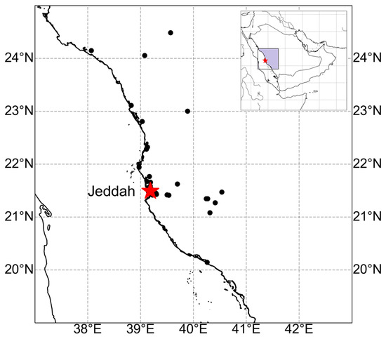
Figure 5.
Locations of the stations used for the evaluation.
The GPM-IMERG-Late [81] dataset is derived from sophisticated algorithms that combine data from many satellite-microwave and infrared precipitation estimates, precipitation gauge analyses, and other estimators. The dataset’s spatial resolution is 0.1 × 0.1 deg, with available temporal frequencies of 30 min.
Across the country, a network of METEOSERVIS MR2-0.2s rain gauges measures liquid precipitation with a resolution of 0.2 mm. These gauges rely on the “tipping bucket” principle, with a catching area of 200 cm2. The range of proper operation is between 0 and 900 mm/hr, and the measuring error depends on the intensity of the rain. The values reported by the manufacturer are under 1% for rain intensity up to 20 mm/hr, <4% between 20 and 60 mm/hr, and <6% between 60 and 200 mm/hr.
For each event, rainfall maps are available based on radar observations from a VAISALA weather radar’s WRM200 network. These devices operate in a frequency range of 5.5 to 5.7 GHz, with an average power of 300 W and peak power of 250 kW (0.12% duty cycle). The transmitters can produce pulses with frequencies ranging between 50 Hz and 2.4 kHz, with two modes of operation, STAR or LDR. The radar receiver employs a dual-stage, dual-channel IF downconverter and digitizer, with a noise figure of less than 2 dB, sensitivity of 3 dB, and dynamic range exceeding 100 dB. Reflectivity values exceeding 80 dB (or 100 dB with waveguide filters) are rejected.
2.3.2. CREST
Given the scarcity of available flood records, our primary objective in tuning the hydrological model was to replicate the shape and peak of observed floods accurately. We divided the tuning procedure into two phases to represent the rapid onset and recession of desert floods accurately. First, we conducted an automatic calibration using the CREST model’s built-in function [64] based on the Shuffled Complex Evolution University of Arizona (SCEUA) algorithm [82]. This algorithm primarily optimizes routing parameters to improve the representation of the shape of the flood hydrograph. The second phase involved a sensitivity analysis within the model to adjust land surface parameters, ensuring they accurately matched the peak flood values. The analysis applied a proportional factor to the initial land surface parameters based on soil properties, land cover types, and canopy profiles [64]. The CREST model’s tuning process utilized one flood record from a 1985 storm over the Wadi Aliath area south of Jeddah (Masood, 2016). We obtained the input forcing data for the calibration process from WRF historical simulations.
The tuned parameters used in the hydrological model are listed in Table 2. The first six parameters are routing parameters. The last parameter, namely CoeSAT, is used to adjust the saturation moisture derived from digital soil mapping data [83] to achieve a comparable runoff coefficient against the observed record in 1985. All routing parameters are within a reasonable range [84], with a high KS value representing the sharp flash flood hydrograph pattern in the desert area.
Table 2.
The tuned routing and land surface parameters of the hydrological model (CREST).
2.3.3. HECRAS
Since no hydrologic observations were available to the authors, we used discharge obtained from the gauge-adjusted radar-rainfall data as a reference to assess the skill of the WRF-based flood forecasts. Observation data for the event comprised reports from people (“crowdsourced”) on localized flood incidents at the street or house level. As highlighted by other authors [85], such observations are often anonymous and/or not georeferenced. Nonetheless, they carry some significant landmarks that allow for pinpointing specific locations from which the images and video were taken. Refs. [86,87] provide a thorough review of studies that used citizen science connected to floods, benchmarking difficulties and benefits of data collection and integration into models. One must consider that retrieving inundation depth/extent from crowdsourced information is subject to biases. Determining water level values from photographs of flooded areas is uncertain due to several factors: (i) the exact size of reference objects in the image may be unknown; (ii) the height of floodwater may vary across different areas of the image; and (iii) objects might be partially visible because they can be submerged in water [88]. Nevertheless, citizen science data can be adequate to provide information for evaluating the performance of the model [85,88,89,90,91,92] and to determine flood extent, as this is generally less uncertain due to its binary nature [85,86,93].
3. Results
3.1. CREST Tuning
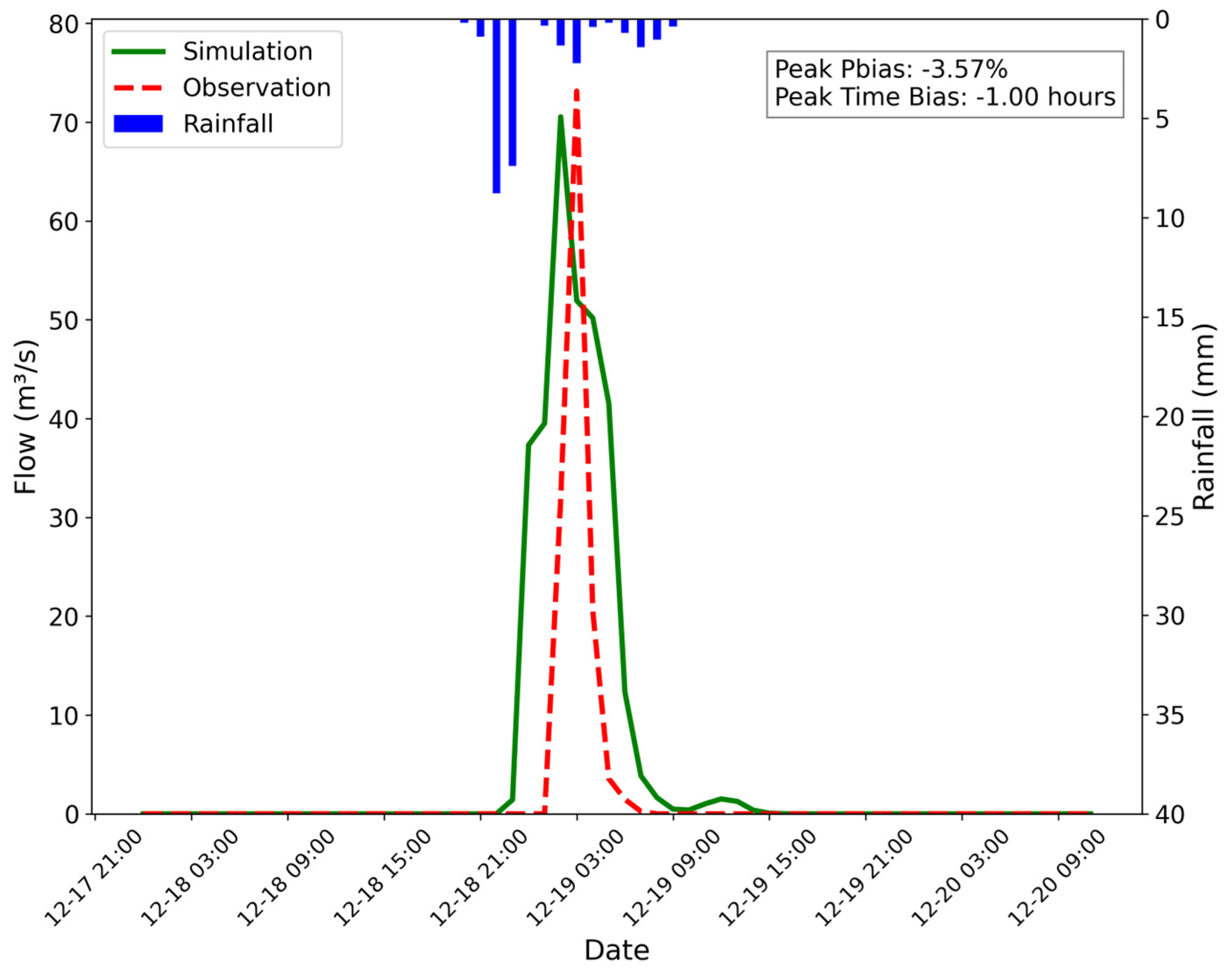
Figure 6 presents the optimally simulated flood hydrograph following the tuning process. The simulation successfully captured the rapid response of the flood to precipitation events, showing a good overall match with the recorded flood data in both the shape and peak values. The produced peak value closely resembled the observed one in amount (−3.6%) and timing (−1.0 h). Both values are indicators of very good performance of the model, as the timing error should ideally be within a small time window, such as ±1–2 h for short-term flood events, and a good value for peak flow percentage should ideally be within ±10–15% of the observed peak flow [77,78,94].
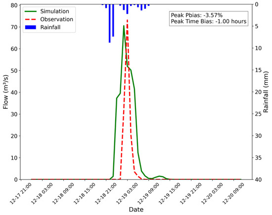
Figure 6.
Simulated flood hydrograph derived from the tuned parameters compared with the observed record for 1985 at the outlet of Wadi_415.
Incorporating more observational data, nonetheless, is encouraged to refine the model calibration further and improve evaluation metrics.
3.2. Validation of WRF Precipitation Predictions
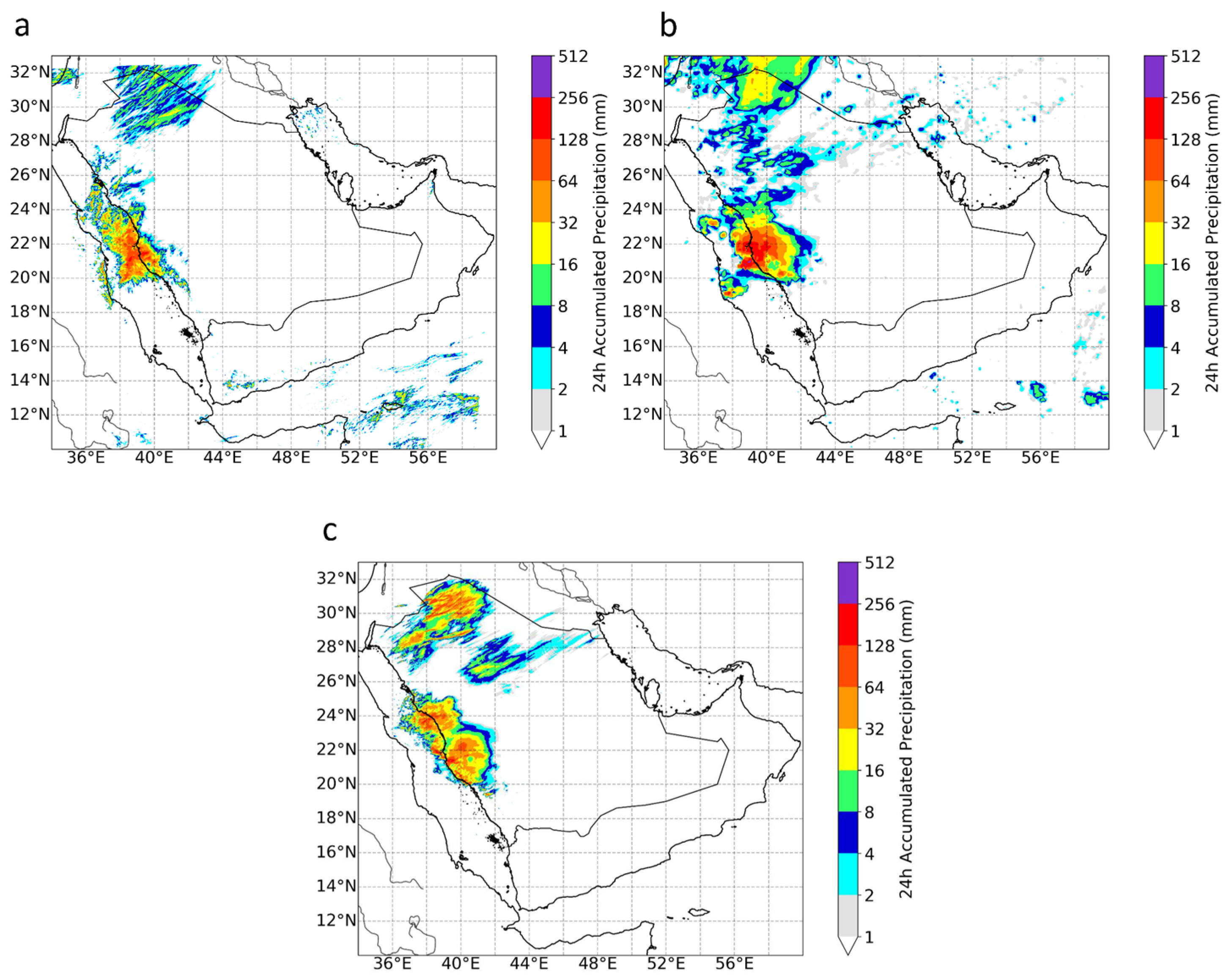
The WRF estimates for the spatial distribution of 24-h accumulated precipitation agreed with radar observations and the IMERG-Late dataset, as shown in Figure 7. In all three products, the accumulated precipitation reached a value of 50 mm. However, it is essential to note that IMERG data consistently overestimated rainfall with respect to radar by a factor of two.
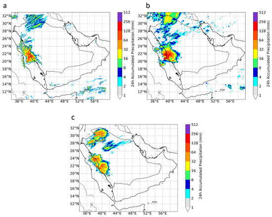
Figure 7.
The 24-h accumulated precipitation for 24 November 2022, as retrieved by (a) WRF, (b) IMERG-Late, and (c) bias-adjusted radar.
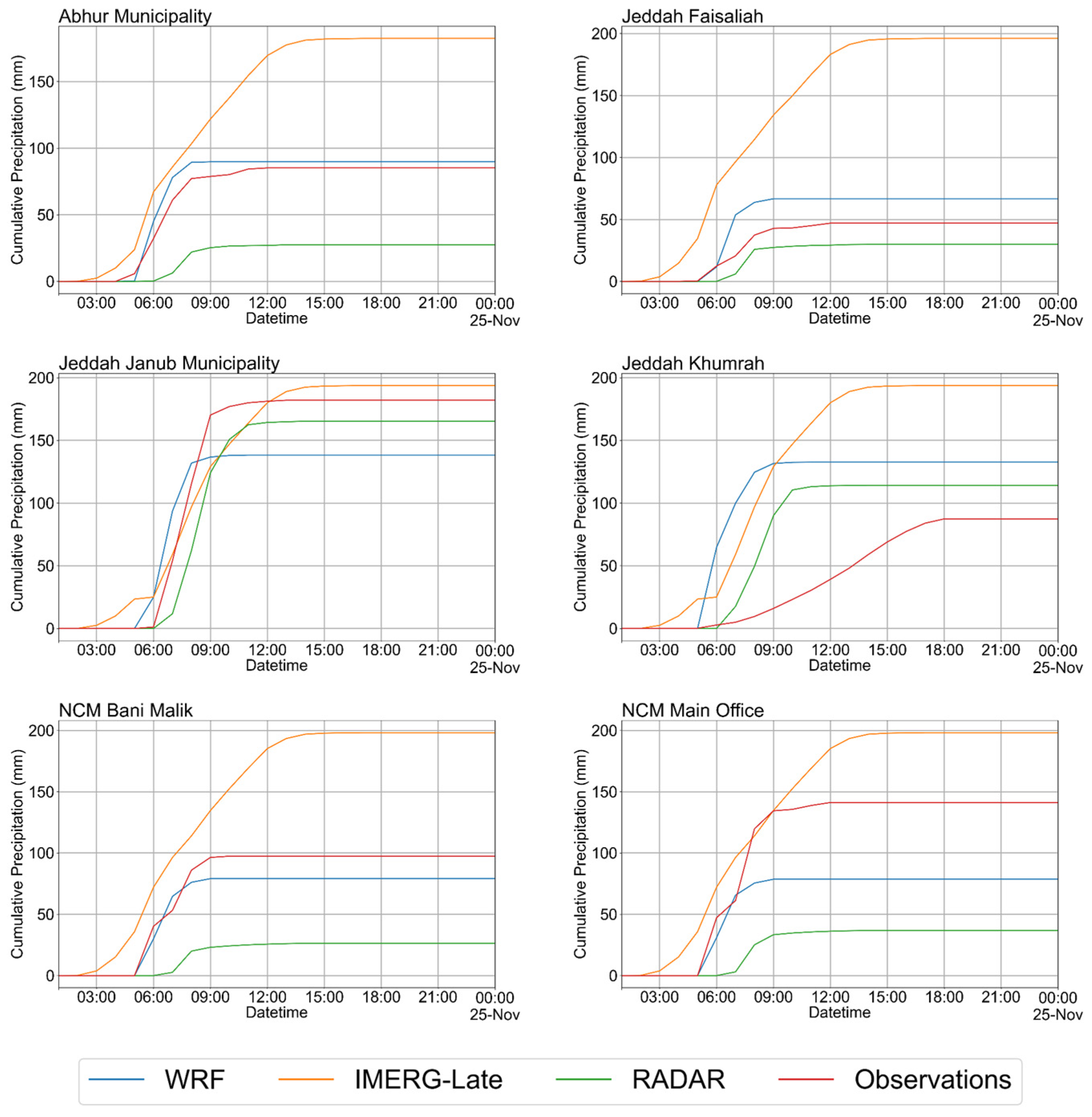
Figure 8 presents a comparison of WRF cumulative precipitation time series. As station observations indicated, a significant amount of rain (up to 180 mm) fell between 03 and 09 UTC on 24 November. In Abhur Municipality, Jeddah Janub Municipality, and NCM Bani Malik, the error of WRF prediction was within 25%. A higher error was recorded for the NCM main office, with an underprediction of 50%. The time series in Figure 8 and the statistical metrics in Table 3 demonstrate the model’s high performance, as the Pearson coefficient was around 0.60. The mean absolute error (MAE) and root mean square error (RMSE) were the lowest for WRF, followed by radar and IMERG, respectively. The bias suggested that WRF overpredicted precipitation by 10% in all stations, while the IMERG dataset did so by 137%. Since the radar product underwent bias adjustment, the bias had a value of 1. Focusing on the model behavior, potential errors and discrepancies in forecasting capacity can be attributed to the highly localized features of the convective activity and the errors induced by the initial and boundary conditions and the physical parameterizations employed in the operational system.
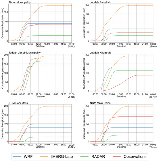
Figure 8.
Cumulative rainfall curves of WRF, IMERG-Late, bias-adjusted radar and station observations.
Table 3.
WRF statistical evaluation against in situ station observations. Readers should refer to Figure 8 for the overall rainfall statistics of the various products, as compared to measured rainfall.
Object analysis has been carried out to compare WRF (forecast) and IMERG dataset (observation), re-gridding all results to 10 km resolution. The analysis is performed by re-griding the model to match the observation resolution (10 km). Figure 9 shows the WRF objects (a), the IMERG (b), and WRF objects (colored) with the IMERG outlines (c). The result identified similar rainfall patterns regarding coverage of the rainfall event, as well as its intensity and location.
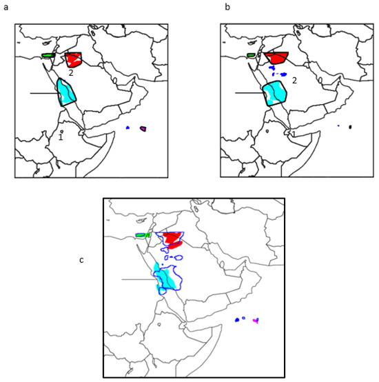
Figure 9.
Object analysis, WRF objects (a), IMERG-Late objects (b), IMERG outlines, and WRF objects (colored). Comparison of the overlapping objects is shown in (c). Object 1 in blue highlights the area of interest of Jeddah, whereas object 2 in red highlights a secondary area of rainfall.
The area of interest, Jeddah, is highlighted in blue in Figure 9, and it is labeled as object no. 1. Table 4 reports the statistics for this object. When comparing the centroid of the area captured by WRF to the one from IMERG, the distance was about 112 km, with a tilt between the axis of 1.1 degrees. The forecast object area covers about 1708 pixels, whereas the observation area was 2200. The intersect in both the 1202 grid and the unmatched area (symmetry difference) is a total of 1504 pixels.
Table 4.
Object analysis statistics between WRF (FCST) and IMERG (OBS). In the table, 1 grid point covers a 10 × 10 km pixel.
For this analysis, IoU is around 0.44, which is consistent, however, with the high overestimation of IMERG compared to radar data. Even though the analysis shows there is a shift in the WRF forecast offshore, the model managed to forecast the rain event of the area covering Jeddah city as a whole. These results highlight how, in addition to capturing the statistics of the rain event itself (Table 4), WRF was also able to capture the overall spatial properties of the storm over the city of Jeddah, providing valuable information for the warning system.
3.3. Validation of CREST-HEC2D Discharge and Inundation Depths
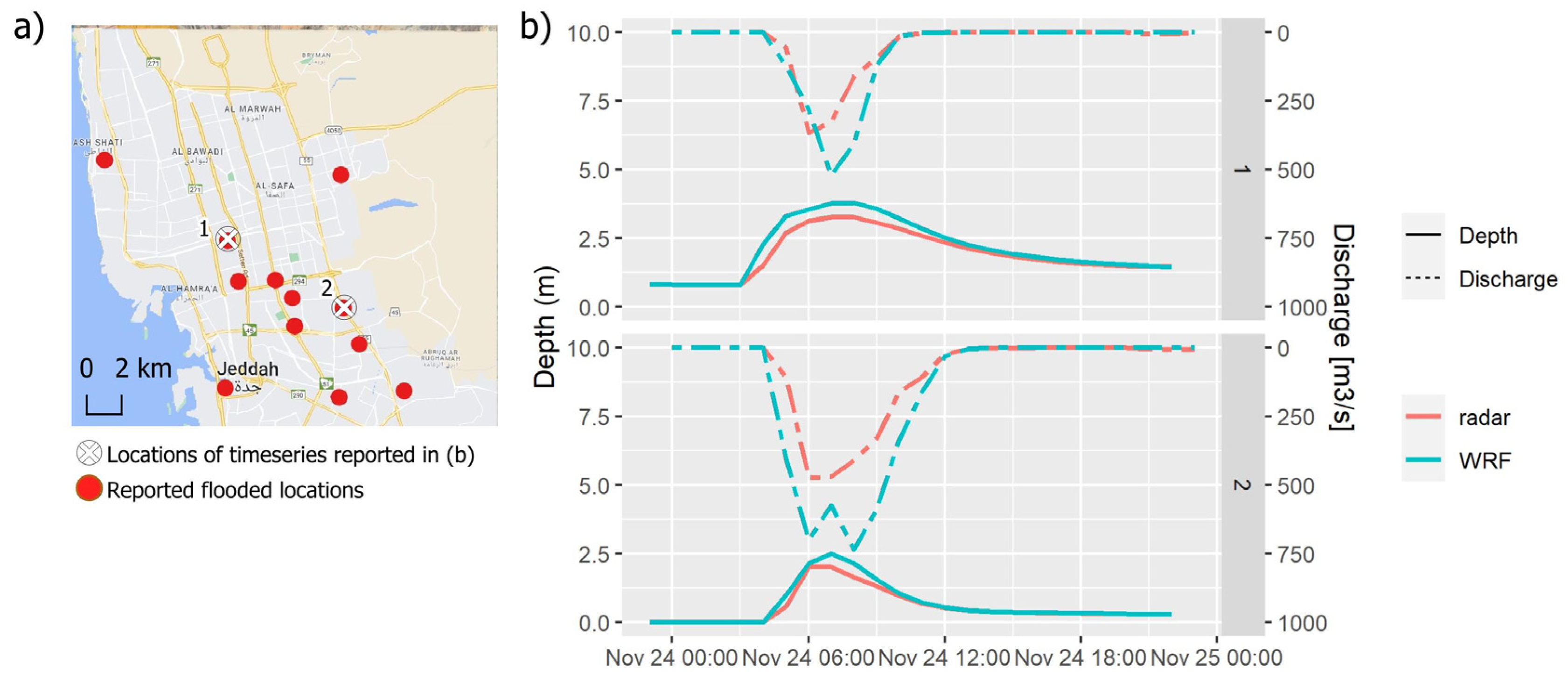
The NCM Flash Flood Forecasting System provided discharge and inundation depths at a one-hour resolution. The flood peak discharge timing, from the hydrological model, was overall consistent (Figure 10), with a slight delay of the peak (<20 min) forecast by WRF for some locations. The timing consistency was also valid for the inundation depth. The WRF forecast captured the maximum depth consistently compared to the radar hindcast. The inundation volume forecast by WRF was slightly higher than that of the radar hindcast, consistent with the differences in peak discharge from CREST (Figure 10). The WRF forecast was triggered on November 23 (the day before the event) at 12.30; the peak discharge was forecast around 8.30 for November 24; and the peak inundation depth nearby was forecast around 9 on November 24, with timing consistent with the peak rainfall measured from the rain gauges (between 03 and 09 UTC on 24 November).
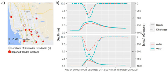
Figure 10.
Comparison between the WRF-based forecast and radar-based simulation. The figure reports the flooded locations (a) and time series of depths and CREST discharge for two selected locations (b).
The spatial depiction of the maximum flood depth (HEC2D), both WRF-based and radar-based (shown in Figure 11a), provided similar overall statistics. The WRF-based forecast produced a slightly higher inundation depth (median = 1.3 m vs. 0.8 m for the radar data), consistent with the peak discharge differences shown in Figure 10. The radar-based inundation captured a lower variability range (0 m–1.5 m overall, compared to a general range of 0 m–3 m for WRF-based simulations). Across the domain (Figure 11b), correspondence between simulated depths from WRF and the radar data was good, with some outliers of inundation >2 m for the WRF-based simulation, as compared to inundations <0.5 m for the radar-based analysis. The comparison of the inundation depth quantiles for the November 24 storm (Figure 11c) indicated agreement between the WRF-forecast peak inundation depths and the radar-derived ones (Figure 11c). The differences between the produced inundation characteristics (percentile of depths) when using WRF versus the radar-based hydrographs were minimal (Figure 11c), with most of the domains presenting excellent agreement.
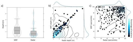
Figure 11.
Inundation depth over Jeddah, as simulated from discharge derived using WRF and radar forcings. The figure shows (a) the overall variability from the boxplots, as well as the density distribution of points across the domain, and the correspondence between WRF and radar data of inundation depth (b) and the percentiles of inundation depth (c).
Apart from the qualitative comparison among all the datasets, we performed a statistical comparison of the model data, further highlighting their good performance (Table 5). The statistical analysis showed good to very good accordance between the WRF forecast and radar hindcast discharge for the CREST model (correlation: 0.95–0.97; NSE: 0.76–0.82), and the results were consistent for the HEC2D model.
Table 5.
CREST-HEC2D statistical evaluation. Statistics were calculated by comparing the WRF-based forecast with the radar-based hindcast. Values are shown for inundation depth considering the whole domain, while for discharge, they refer to the selected locations displayed in Figure 11.
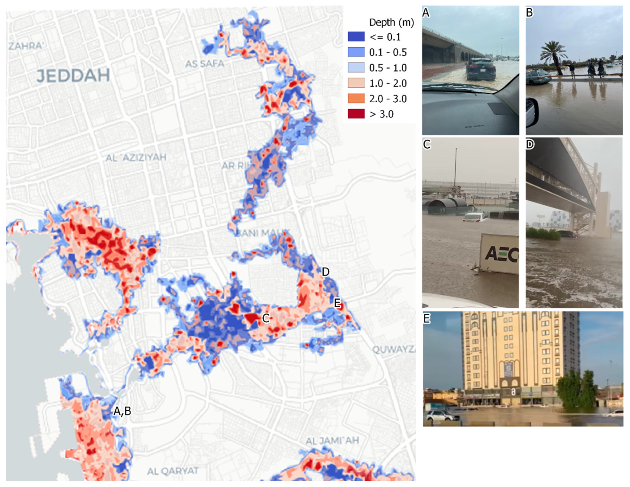
We also found good agreement in comparing the forecast depths with reported flooded locations (Figure 12). We estimated the water depth at each location by relating it to objects shown in the pictures, such as car tires, walls, traffic signs, or significant landmarks. Most locations displayed good visual correlation with the WRF-forecast depths. In Figure 12, images A and B show inundation reaching the car tires, indicating less than 0.5 m of water, comparable to the simulated depth. Some areas also showed very high inundation (>1 m), and citizen-sourced videos showcased major flooding (C, D).
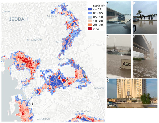
Figure 12.
WRF-based forecasted depth, compared to selected crowdsourced videos. Letters A to E reports the location of each crowdsourced image on the right-hand side of the figure.
4. Discussion
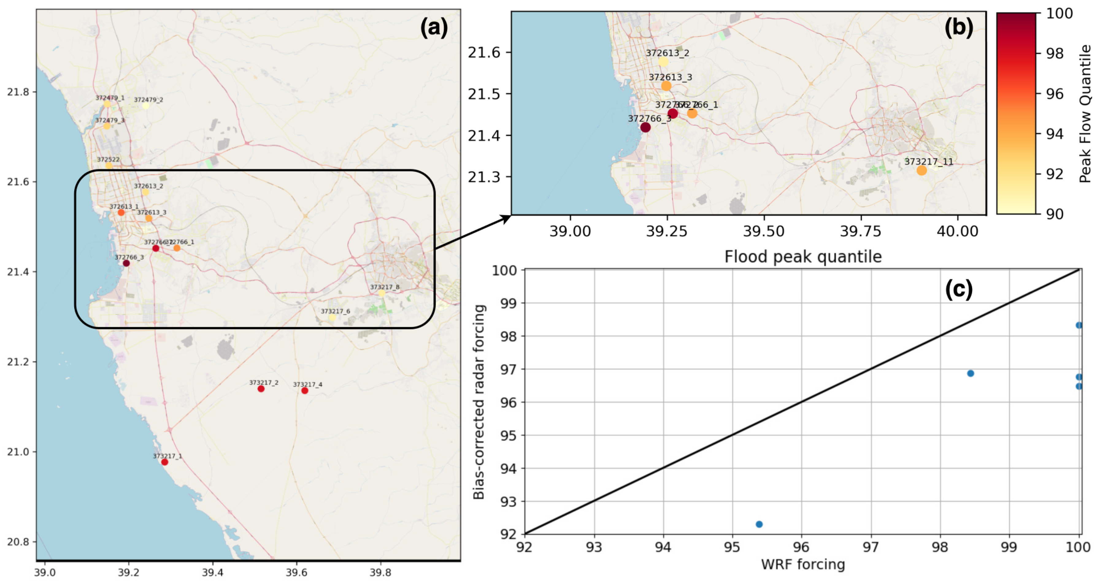
Because flood discharge observations were unavailable to the authors, we utilized flood simulation forced by gauge-adjusted radar-rainfall as a reference to assess the accuracy of the flood forecasts based on the WRF. The results demonstrated that WRF-derived precipitation enhanced the flood early warning system more significantly than radar-based precipitation. The comparison of the flood quantiles for the 24 November flood event, as depicted in Figure 13, showed close alignment of the peak discharge quantiles forecast by the WRF model with those derived from the radar-based approach. The differences between the flood characteristics (hydrographs peaks) when using WRF and the radar-based predictions were minimal (see Figure 13). Overall, the forecast river discharge for the event was within the range of >95%, especially in the southern part of the city.

Figure 13.
CREST outlets. Quantiles of discharge from WRF forecast (a) compared to those obtained from radar data (b). One-to-one comparison for selected outlets is also shown (c).
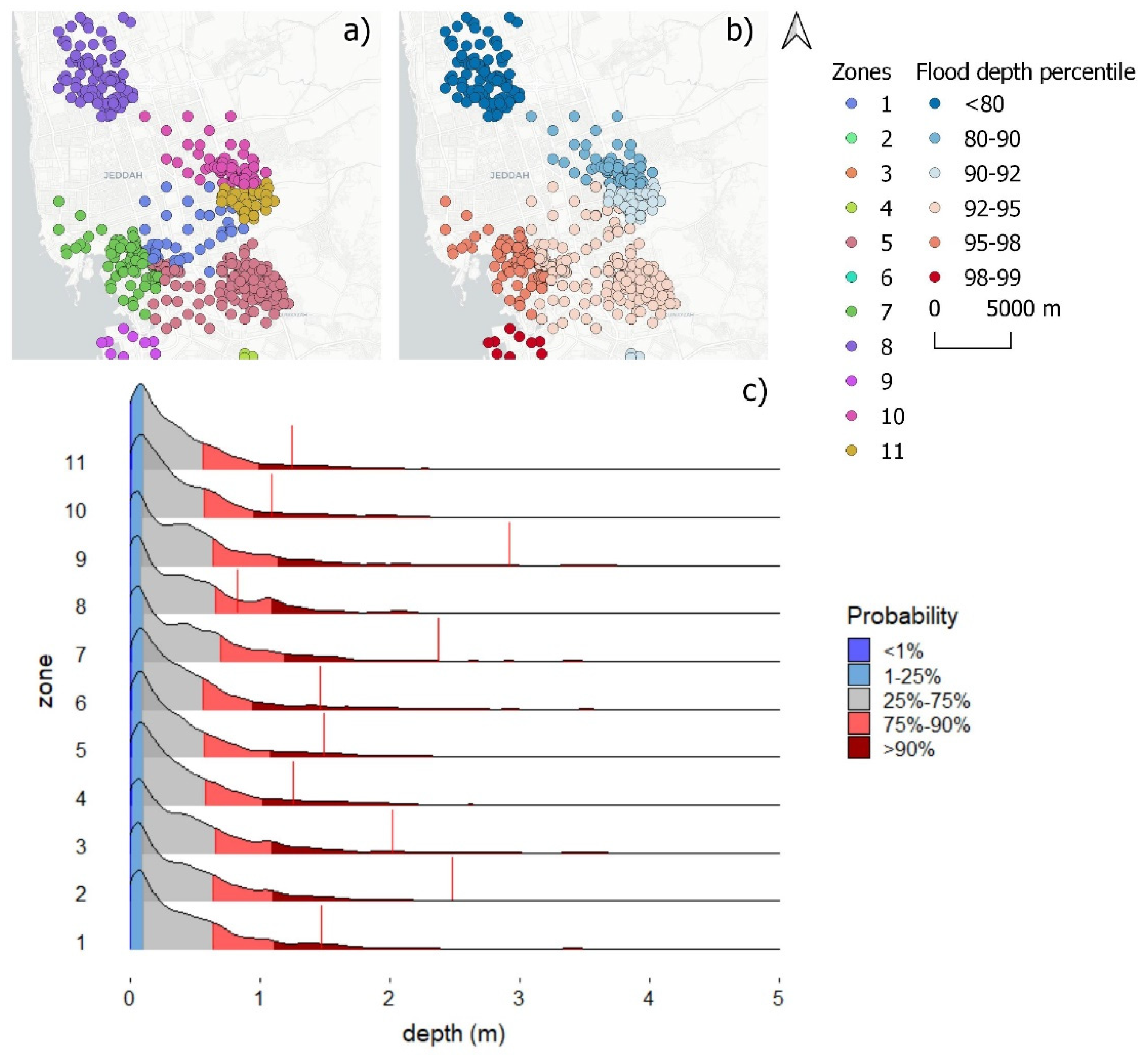
We retrieved hourly inundation values for 50 historical floods in the area from 2000 to 2017 for over 7000 hourly depth maps and randomly sampled the inundation extents in areas downstream of the CREST outlets (Figure 14c). Consistent with the high flow quantiles, the southern part of Jeddah experienced the highest quantiles of inundation depths during the November 2022 event (Figure 14b), with the highest near the coastline (zone 9 in Figure 14).

Figure 14.
Inundation quantiles at selected locations. Neighboring zones (a) and quantiles of flood depth (b) compared to the historical distribution of depths for the same areas (c). The red line in (c) indicates the most frequent depth within those areas for the November 2022 event.
4.1. Performance of the Flood Warning System in Jeddah in November 2022
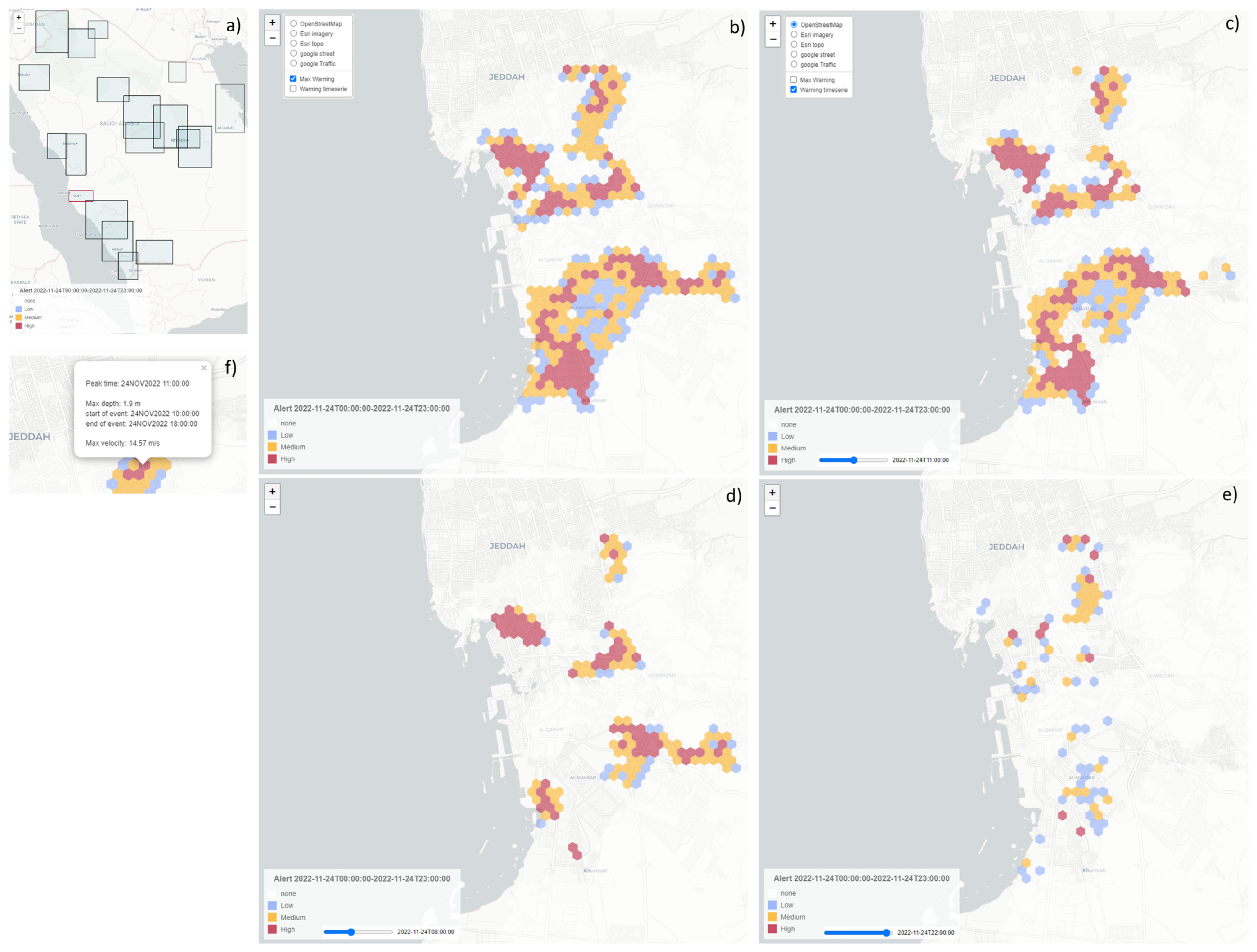
Although some regions are more prone to flooding than others, implementing flood warning systems over major cities is essential to deliver information vital to safeguarding property and preserving lives. As installing gauges and telemetry equipment in such a vast environment is not feasible, effective flood warning strategies require skilled personnel and well-designed protocols to offer early warning about the likelihood, timing, and severity of floods. Figure 15 showcases the warning system provided during the November 2022 event. Authorities have (as they did then) access to a global warning map (Figure 15a), with each domain color-coded across the country based on warning levels expected from the most recent forecast cycle. The web system is updated every six hours, allowing access to the three most recent warning maps.
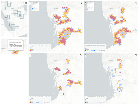
Figure 15.
Warning system available to the authorities: overall warning (a), maximum warning for the event (b), and warning time series at different moments of the available simulation window (c–e). The available information for each hexagon is shown in (f).
Clicking on the domain makes the warnings visible both in a static way (Figure 15b) and, after receiving feedback for the event, dynamically (Figure 15c–e). The warning maps trade off geographic realism for equalizing the importance of each region under investigation and allow highlighting locations where inundation depth is increasing. Warning levels depend on three depth thresholds: 0.2 m, 0.5 m, and 1 m. Anything below 0.2 m is issued a “low” warning. Conversely, anything above 1 m prompts a “high” warning.
For the static approach (Figure 15b), the meter-scale, hourly flood-depth maps are transformed into a maximum inundation. Each hexagon is then attributed the mode of the absolute maximum inundation, considering all pixels within its coverage, and the mode is rounded down to the closest warning level. This procedure is repeated for the dynamic approach (Figure 15c–e), aggregating the hourly depths over a 12-h window and providing the maximum inundation every 12 h.
Given that the forecast window covers five days, defining the beginning and end of the forecast inundation is critical. For this, as well as for the static maximum warning maps, the system is constructed to allow the retrieval of the following at each available timestep: (i) the most common inundation level inside each hexagon; (ii) the earliest expected peak time (that is when the water reaches its maximum flood depth); (iii) the latest recession time (when the water depth recedes below the specified warning level); and (iv) the flow velocity (the hotspot in Figure 15f).
To obtain a clearer idea of the exposure for each location, trained personnel in charge of the warning system can select various base maps, including Google Traffic, Google Imagery, and OpenMP cartography, as background.
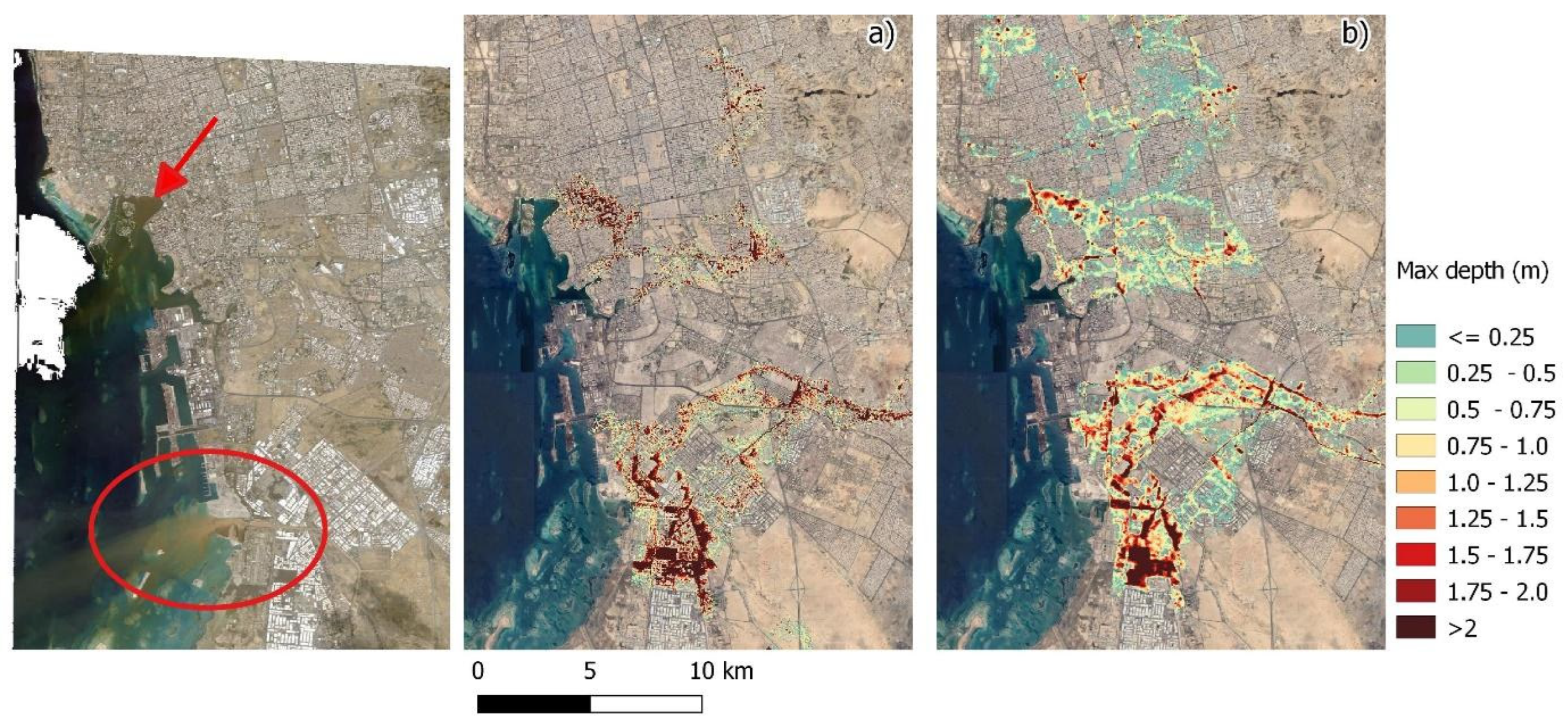
A key characteristic that significantly affects flood inundation simulations is the resolution of the input terrain [95,96]. While its exceptional accuracy makes LiDAR the most preferred terrain for flood studies, its widespread adoption is hindered by its high production costs. Consequently, regional flood studies often turn to global terrain data, which are more accessible and affordable. For this work, the COP-30 DEM provided the most suitable and computationally inexpensive source of data, which outweighed its medium resolution (30 m; Figure 16a). Overall, since the landscape under investigation was primarily free of vegetation, COP30 worked well in representing topography, including buildings and infrastructure, and thus captured the evolution of the flood (Figure 16a). Comparisons of the WRF-forecast-based inundation area with a satellite view taken over Jeddah by PLÉIADES NEO SATELLITE on November 25 at 8.30 UTC showed that the highest floodwater accumulation provided by the flood forecast system corresponded with locations where sediment was delivered to the sea in the aftermath of the event, confirming the likelihood of the flooding for these areas. Looking at the inundation derived using the higher-resolution terrain (2.5 m, Figure 16b), the system provided a larger flooded area than the coarser-resolution DEM (Figure 16a). The goodness of the terrain model is known to depend on the severity of events and modeling purposes [97]; overall, the finer-resolution DEM appears to have performed better for reproducing small flows associated with smaller inundation depths, such as the widespread inundation with depths of less than 0.25 m, highlighted in Figure 16b. Nonetheless, overall, the flood patterns were similar between the two models.
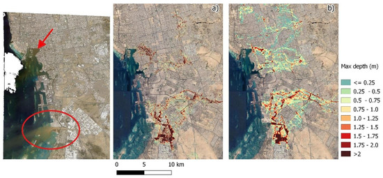
Figure 16.
Detailed comparison of the WRF-based flood inundation using the 30 m DEM (a) and the 2.5 m high-resolution one (b). The left panel image shows a satellite view taken over Jeddah on November 25 at 8.30 UTC by PLÉIADES NEO SATELLITE. While it is not possible to detect the actual flood extent, the image shows sediment being delivered to the sea, highlighted by the red arrow and circle, with input from the locations where the flood forecast system showed the highest floodwater accumulation.
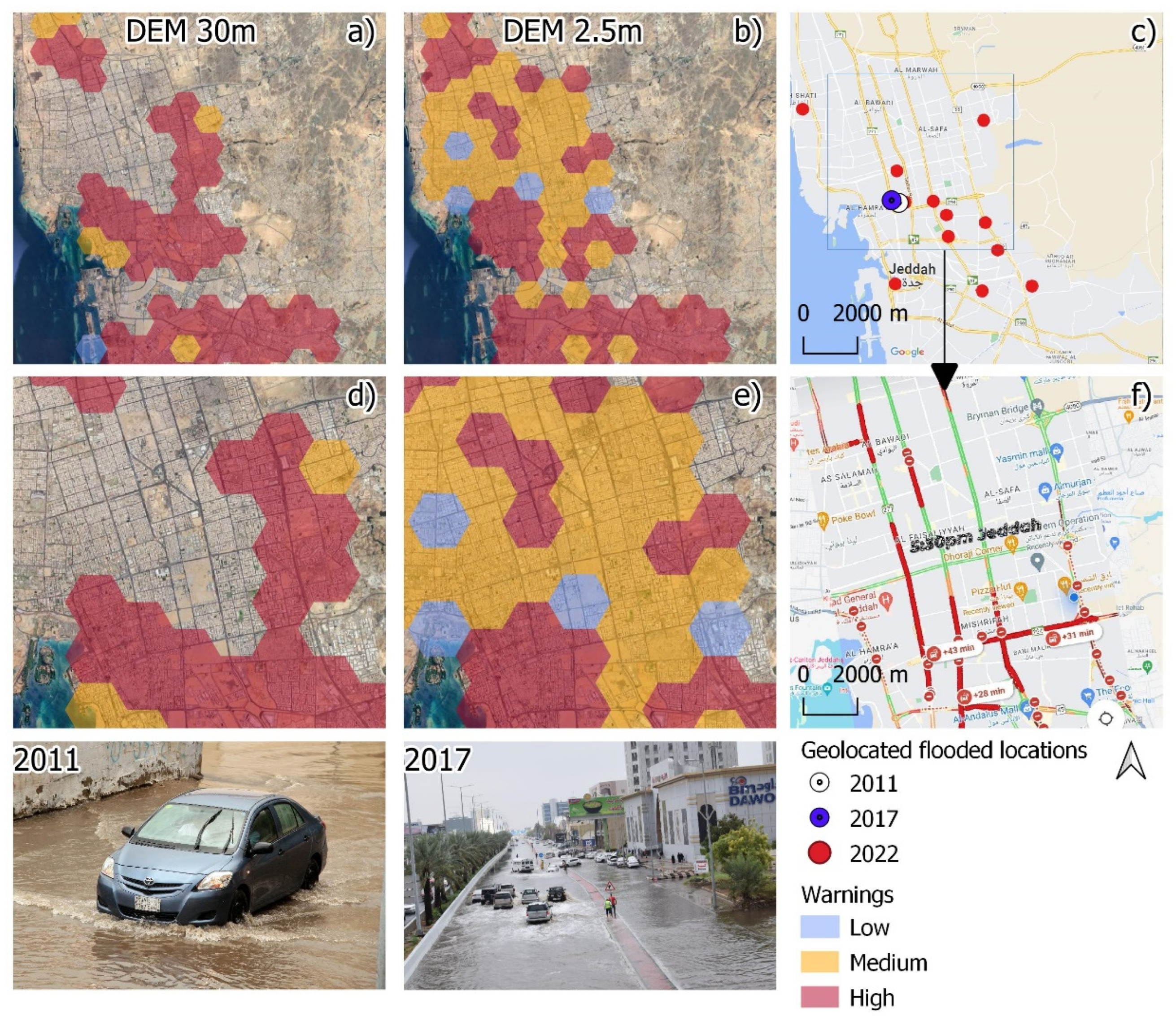
Because of a lack of independent flood inundation data on the event, only anecdotal evidence was available to compare the warning data. Nonetheless, the comparison (Figure 17) suggested that the system performed well in identifying high-risk areas, using both the 30 m DEM and the 2.5 m DEM for the simulation. Despite not having much crowdsourced feedback for many historical events in the area, it is noted that some high-warning areas were identified as high risk for the November 2022 event, and they historically reported flooding in 2017 and 2011. Consistent with what was highlighted in the previous section, the high-resolution terrain (aw3d) provided more extensive coverage of high warning areas than the coarser-resolution DEM (Figure 17b,e versus Figure 17a,d). The combination of the two DEM resolutions allowed for labeling with high and medium warnings in most of the flooded locations and areas where traffic jams indicated possible flooding (Figure 17c,f).
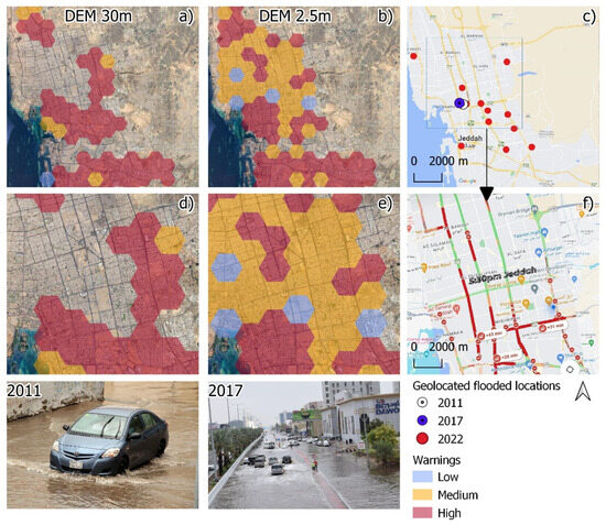
Figure 17.
WRF-based flood warnings from 30 m (a,d) and 2.5 m DEM (b,e), as compared to flooded locations crowdsourced on November 24–25 (c) and traffic on November 24 (f). Crowdsourced flooding for 2011 and 2017 is also reported. (c,f) are from Flickr; credits to Efren Rodriguez (2011) and Saidalavi Mohamed (2017).
4.2. Remarks
Even if a forecast system functions technically, many “potential deficiencies” exist at each stage that must be kept in mind to avoid hindering the effectiveness of the warning model [98]. It is essential not only for local disaster management and authorities to receive and notice a warning in time but also to understand its content [99,100]. Together with the implemented warning system, we provided basic training to its users, including a fundamental understanding of hydrology and hydraulics, hydraulic modeling, and manipulation of terrain data for properly addressing urban features within hydraulic models, and deep training on how to interpret the results of the model simulations and, if needed, retrieve past warnings. Having conveyed a proper grasp of the system, it was also possible to highlight its limitations, which were inherent in building a countrywide flood system with very scarce field-based data for validation. Trained personnel had access to both past warning maps and the maps for the 2022 event and could highlight areas where the model did not provide sufficient coverage. One must consider that the initial selection of the outlets for the hydrological model and, therefore, the upstream boundary conditions of the hydraulic model were arbitrary and determined by overlaying the urban area extent with the river network in each subbasin. Using Google Maps, the locations of the outlets were then adjusted to areas where we could find extensive infrastructure and where we expected more difficulties in simulating hydraulic flows. Based on the feedback from the trained personnel, we could increase the outlet density for the current system.
A central point to consider is that the streamflow simulation of the CREST model would be further enhanced by expanding the calibration process for various regions across the country. At present, CREST calibration relies on limited observational records from restricted locations. As a result, the current parameters may not comprehensively capture flood patterns across all of Saudi Arabia for every flood. We believe that we can extend the calibration procedure to more areas by securing additional flood observation records or acquiring detailed feedback from actual events. This would provide the model with richer localized information, ensuring more precise and representative streamflow simulations.
Finally, we conducted roundtables with the involved personnel to obtain information and learn their questions, uncertainties, and concerns in connection with three descriptive methods: flow quantiles versus amounts, inundation depths, and warning maps. Their feedback and our qualitative observation revealed a disjuncture between, on the one hand, understanding and using warnings based on a statistical (inundation percentiles) method and, on the other, a preference for concrete references in describing risk in terms of warnings based on actual depths. This was consistent with studies conducted in other environments [101].
5. Conclusions
This research assessed the performance of an operational national-scale flash flood forecasting system for the Kingdom of Saudi Arabia during a severe precipitation event in Jeddah on 24 November 2022, the most intense ever documented in the region. This event resulted in widespread flash floods affecting both urban and rural areas of Jeddah.
The study compared the atmospheric component forecast with the NASA satellite precipitation product (IMERG-Late) and radar-based rainfall estimates, adjusted for bias using in situ gauge observations. Because hydrological observations were absent, we utilized as a reference the discharge predicted from our system using input gauge-adjusted radar-rainfall estimates, which represent the benchmark precipitation, to evaluate the accuracy of the flood forecasts based on the Weather Research and Forecasting (WRF) model. Additionally, the study evaluated the effectiveness of the warning system by comparing its forecasts to publicly reported information on localized flood incidents at the street or neighborhood level obtained through “crowdsourcing.”
The findings indicated a temporal and spatial agreement between the forecast precipitation from WRF and the bias-adjusted radar-rainfall estimates. In contrast, the IMERG-Late data tended to overestimate precipitation in alignment with previous satellite validation studies. The comparison of flood quantiles for the November 24 event revealed a close correspondence between the WRF-driven flood peak discharge properties and those derived based on the gauge-adjusted radar-rainfall estimates. Minimal differences were observed in flood characteristics (such as hydrograph peak, timing, and volume) when using WRF-forecast precipitation versus radar-based benchmark data. The simulated inundation effectively captured broad flooding patterns at the city level, with over 95% of reported incidents in city districts falling within the areas for which the operational system provided high or extreme warnings on November 23—more than 12 h in advance.
The importance of the Flash Flood Forecast System for Saudi Arabia cannot be overstated. In a region prone to sudden and intense rainfall events, the system is a proactive tool for disaster risk reduction. Providing accurate and timely forecasts empowers communities to prepare and respond effectively, ultimately saving lives and minimizing the impact of flooding on infrastructure. As demonstrated by its success during the Jeddah event, the system presents an efficient solution for forecasting the potential impacts of extreme rainfall events, particularly those that can cause significant flash floods in the urban areas of Saudi Arabia.
Author Contributions
Conceptualization, G.S., Q.Y., X.S., M.F.M., P.P., I.C., A.K., M.A.A., S.S.A., Z.C. and E.A.; methodology, G.S., Q.Y., X.S., M.F.M., P.P., I.C., A.K., M.A.A., S.S.A., Z.C. and E.A.; software, G.S., Q.Y., X.S. and P.P.; validation, G.S., Q.Y., X.S., M.F.M., P.P., I.C., A.K., M.A.A., S.S.A., Z.C. and E.A.; formal analysis, G.S., Q.Y., X.S., M.F.M., P.P., I.C., A.K., M.A.A., S.S.A., Z.C. and E.A.; investigation, G.S., Q.Y., X.S., M.F.M., P.P., I.C., A.K., M.A.A., S.S.A., Z.C. and E.A.; resources, Z.C., M.A.A. and S.S.A.; data curation, G.S., Q.Y., X.S., M.F.M., P.P., I.C., A.K., M.A.A., S.S.A., Z.C. and E.A.; writing—original draft preparation, writing—review and editing, visualization, G.S., Q.Y., X.S., M.F.M., P.P., I.C., A.K., M.A.A., S.S.A., Z.C. and E.A.; supervision, E.A.; project administration, E.A.; funding acquisition, E.A. All authors have read and agreed to the published version of the manuscript.
Funding
Funding for this study was provided by a project supported by the National Center for Meteorology of the Kingdom of Saudi Arabia.
Data Availability Statement
The raw data supporting the conclusions of this article will be made available by the authors on request if not covered by copyrights.
Conflicts of Interest
Emmanouil Anagnostou declares that he holds stock in FloodInov LLC. Zaphiris Christidis declares that he holds stock in Lenovo. Andreas Kallos declares that he holds stock in Weather & Marine Engineering Technologies P.C. The remaining authors declare that the research was conducted in the absence of any commercial or financial relationships that could be construed as a potential conflict of interest.
References
- Dottori, F.; Szewczyk, W.; Ciscar, J.-C.; Zhao, F.; Alfieri, L.; Hirabayashi, Y.; Bianchi, A.; Mongelli, I.; Frieler, K.; Betts, R.A.; et al. Increased Human and Economic Losses from River Flooding with Anthropogenic Warming. Nat. Clim. Chang. 2018, 8, 781–786. [Google Scholar] [CrossRef]
- Hirabayashi, Y.; Tanoue, M.; Sasaki, O.; Zhou, X.; Yamazaki, D. Global Exposure to Flooding from the New CMIP6 Climate Model Projections. Sci. Rep. 2021, 11, 3740. [Google Scholar] [CrossRef]
- Hirabayashi, Y.; Mahendran, R.; Koirala, S.; Konoshima, L.; Yamazaki, D.; Watanabe, S.; Kim, H.; Kanae, S. Global Flood Risk under Climate Change. Nat. Clim Chang. 2013, 3, 816–821. [Google Scholar] [CrossRef]
- Kimura, Y.; Hirabayashi, Y.; Kita, Y.; Zhou, X.; Yamazaki, D. Methodology for Constructing a Flood-Hazard Map for a Future Climate. Hydrol. Earth Syst. Sci. 2023, 27, 1627–1644. [Google Scholar] [CrossRef]
- Cutter, S.L.; Emrich, C.T.; Gall, M.; Reeves, R. Flash Flood Risk and the Paradox of Urban Development. Nat. Hazards Rev. 2018, 19, 05017005. [Google Scholar] [CrossRef]
- Hapuarachchi, H.A.P.; Wang, Q.J.; Pagano, T.C. A Review of Advances in Flash Flood Forecasting. Hydrol. Process. 2011, 25, 2771–2784. [Google Scholar] [CrossRef]
- Khajehei, S.; Ahmadalipour, A.; Shao, W.; Moradkhani, H. A Place-Based Assessment of Flash Flood Hazard and Vulnerability in the Contiguous United States. Sci. Rep. 2020, 10, 448. [Google Scholar] [CrossRef] [PubMed]
- Hinge, G.; Hamouda, M.A.; Long, D.; Mohamed, M.M. Hydrologic Utility of Satellite Precipitation Products in Flood Prediction: A Meta-Data Analysis and Lessons Learnt. J. Hydrol. 2022, 612, 128103. [Google Scholar] [CrossRef]
- Zander, M.J.; Viguurs, P.J.; Sperna Weiland, F.C.; Weerts, A.H. Future Changes in Flash Flood Frequency and Magnitude over the European Alps. Hydrol. Earth Syst. Sci. Discuss. 2022, 2022, 1–21. [Google Scholar] [CrossRef]
- Fekete, A.; Sandholz, S. Here Comes the Flood, but Not Failure? Lessons to Learn after the Heavy Rain and Pluvial Floods in Germany 2021. Water 2021, 13, 3016. [Google Scholar] [CrossRef]
- Petrucci, O. Review Article: Factors Leading to the Occurrence of Flood Fatalities: A Systematic Review of Research Papers Published between 2010 and 2020. Nat. Hazards Earth Syst. Sci. 2022, 22, 71–83. [Google Scholar] [CrossRef]
- Acosta-Coll, M.; Ballester-Merelo, F.; Martinez-Peiró, M.; De la Hoz-Franco, E. Real-Time Early Warning System Design for Pluvial Flash Floods-A Review. Sensors 2018, 18, 2255. [Google Scholar] [CrossRef] [PubMed]
- Witze, A. Why Extreme Rains Are Gaining Strength as the Climate Warms. Nature 2018, 563, 458–460. [Google Scholar] [CrossRef] [PubMed]
- Yin, J.; Gao, Y.; Chen, R.; Yu, D.; Wilby, R.; Wright, N.; Ge, Y.; Bricker, J.; Gong, H.; Guan, M. Flash Floods: Why Are More of Them Devastating the World’s Driest Regions? Nature 2023, 615, 212–215. [Google Scholar] [CrossRef]
- Borga, M.; Gaume, E.; Creutin, J.D.; Marchi, L. Surveying Flash Floods: Gauging the Ungauged Extremes. Hydrol. Process. 2008, 22, 3883–3885. [Google Scholar] [CrossRef]
- Siccardi, F.; Boni, G.; Ferraris, L.; Rudari, R. A Hydrometeorological Approach for Probabilistic Flood Forecast. J. Geophys. Res. Atmos. 2005, 110. [Google Scholar] [CrossRef]
- Georgakakos, K.P. On the Design of National, Real-Time Warning Systems with Capability for Site-Specific, Flash-Flood Forecasts. Bull. Am. Meteorol. Soc. 1986, 67, 1233–1239. [Google Scholar] [CrossRef]
- Yano, J.-I.; Ziemiański, M.Z.; Cullen, M.; Termonia, P.; Onvlee, J.; Bengtsson, L.; Carrassi, A.; Davy, R.; Deluca, A.; Gray, S.L.; et al. Scientific Challenges of Convective-Scale Numerical Weather Prediction. Bull. Am. Meteorol. Soc. 2018, 99, 699–710. [Google Scholar] [CrossRef]
- Marchi, L.; Borga, M.; Preciso, E.; Gaume, E. Characterisation of Selected Extreme Flash Floods in Europe and Implications for Flood Risk Management. J. Hydrol. 2010, 394, 118–133. [Google Scholar] [CrossRef]
- Bannister, R.N.; Chipilski, H.G.; Martinez-Alvarado, O. Techniques and Challenges in the Assimilation of Atmospheric Water Observations for Numerical Weather Prediction towards Convective Scales. Q. J. R. Meteorol. Soc. 2020, 146, 1–48. [Google Scholar] [CrossRef]
- Hu, G.; Dance, S.L.; Bannister, R.N.; Chipilski, H.G.; Guillet, O.; Macpherson, B.; Weissmann, M.; Yussouf, N. Progress, Challenges, and Future Steps in Data Assimilation for Convection-Permitting Numerical Weather Prediction: Report on the Virtual Meeting Held on 10 and 12 November 2021. Atmos. Sci. Lett. 2023, 24, e1130. [Google Scholar] [CrossRef]
- Gourley, J.J.; Flamig, Z.L.; Vergara, H.; Kirstetter, P.-E.; Clark, R.A.; Argyle, E.; Arthur, A.; Martinaitis, S.; Terti, G.; Erlingis, J.M.; et al. The FLASH Project: Improving the Tools for Flash Flood Monitoring and Prediction across the United States. Bull. Am. Meteorol. Soc. 2017, 98, 361–372. [Google Scholar] [CrossRef]
- Price, D.; Hudson, K.; Boyce, G.; Schellekens, J.; Moore, R.J.; Clark, P.; Harrison, T.; Connolly, E.; Pilling, C. Operational Use of a Grid-Based Model for Flood Forecasting. Proc. Inst. Civ. Eng.—Water Manag. 2012, 165, 65–77. [Google Scholar] [CrossRef]
- Zanchetta, A.D.L.; Coulibaly, P. Recent Advances in Real-Time Pluvial Flash Flood Forecasting. Water 2020, 12, 570. [Google Scholar] [CrossRef]
- Douinot, A.; Roux, H.; Garambois, P.-A.; Larnier, K.; Labat, D.; Dartus, D. Accounting for Rainfall Systematic Spatial Variability in Flash Flood Forecasting. J. Hydrol. 2016, 541, 359–370. [Google Scholar] [CrossRef]
- Qi, W.; Ma, C.; Xu, H.; Chen, Z.; Zhao, K.; Han, H. A Review on Applications of Urban Flood Models in Flood Mitigation Strategies. Nat. Hazards 2021, 108, 31–62. [Google Scholar] [CrossRef]
- Krajewski, W.F.; Ceynar, D.; Demir, I.; Goska, R.; Kruger, A.; Langel, C.; Mantilla, R.; Niemeier, J.; Quintero, F.; Seo, B.-C.; et al. Real-Time Flood Forecasting and Information System for the State of Iowa. Bull. Am. Meteorol. Soc. 2017, 98, 539–554. [Google Scholar] [CrossRef]
- Gaume, E.; Bain, V.; Bernardara, P.; Newinger, O.; Barbuc, M.; Bateman, A.; Blaškovičová, L.; Blöschl, G.; Borga, M.; Dumitrescu, A.; et al. A Compilation of Data on European Flash Floods. J. Hydrol. 2009, 367, 70–78. [Google Scholar] [CrossRef]
- Morales-Hernández, M.; Sharif, M.B.; Gangrade, S.; Dullo, T.T.; Kao, S.-C.; Kalyanapu, A.; Ghafoor, S.K.; Evans, K.J.; Madadi-Kandjani, E.; Hodges, B.R. High-Performance Computing in Water Resources Hydrodynamics. J. Hydrol. 2020, 22, 1217–1235. [Google Scholar] [CrossRef]
- Rasiya Koya, S.; Giron, N.V.; Rojas, M.; Mantilla, R.; Harvey, K.; Ceynar, D.; Quintero, F.; Krajewski, W.F.; Roy, T. Applicability of a Flood Forecasting System for Nebraska Watersheds. Environ. Model. Softw. 2023, 164, 105693. [Google Scholar] [CrossRef]
- Sampson, C.C.; Smith, A.M.; Bates, P.D.; Neal, J.C.; Alfieri, L.; Freer, J.E. A High-resolution Global Flood Hazard Model. Water Resour. Res. 2015, 51, 7358–7381. [Google Scholar] [CrossRef]
- Wei, J.; Luo, X.; Huang, H.; Liao, W.; Lei, X.; Zhao, J.; Wang, H. Enable High-Resolution, Real-Time Ensemble Simulation and Data Assimilation of Flood Inundation Using Distributed GPU Parallelization. J. Hydrol. 2023, 619, 129277. [Google Scholar] [CrossRef]
- Hawker, L.; Uhe, P.; Paulo, L.; Sosa, J.; Savage, J.; Sampson, C.; Neal, J. A 30 m Global Map of Elevation with Forests and Buildings Removed. Environ. Res. Lett. 2022, 17, 024016. [Google Scholar] [CrossRef]
- Munawar, H.S.; Hammad, A.W.A.; Waller, S.T. Remote Sensing Methods for Flood Prediction: A Review. Sensors 2022, 22, 960. [Google Scholar] [CrossRef] [PubMed]
- Schumann, G.; Giustarini, L.; Tarpanelli, A.; Jarihani, B.; Martinis, S. Flood Modeling and Prediction Using Earth Observation Data. Surv. Geophys. 2023, 44, 1553–1578. [Google Scholar] [CrossRef]
- Patlakas, P.; Stathopoulos, C.; Flocas, H.; Bartsotas, N.S.; Kallos, G. Precipitation Climatology for the Arid Region of the Arabian Peninsula—Variability, Trends and Extremes. Climate 2021, 9, 103. [Google Scholar] [CrossRef]
- Al-Wathinani, A.M.; Barten, D.G.; Borowska-Stefańska, M.; Gołda, P.; AlDulijan, N.A.; Alhallaf, M.A.; Samarkandi, L.O.; Almuhaidly, A.S.; Goniewicz, M.; Samarkandi, W.O.; et al. Driving Sustainable Disaster Risk Reduction: A Rapid Review of the Policies and Strategies in Saudi Arabia. Sustainability 2023, 15, 10976. [Google Scholar] [CrossRef]
- Ameur, F. Floods in Jeddah, Saudi Arabia: Unusual Phenomenon and Huge Losses. What Prognoses. E3S Web Conf. 2016, 7, 04019. [Google Scholar] [CrossRef]
- Azzam, A.; Ali, A.B. Urban Sprawl in Wadi Goss Watershed (Jeddah City/Western Saudi Arabia) and Its Impact on Vulnerability and Flood Hazards. J. Geogr. Inf. Syst. 2019, 11, 371–388. [Google Scholar] [CrossRef]
- Bashir, B. Morphometric Parameters and Geospatial Analysis for Flash Flood Susceptibility Assessment: A Case Study of Jeddah City along the Red Sea Coast, Saudi Arabia. Water 2023, 15, 870. [Google Scholar] [CrossRef]
- Elsebaie, I.H.; Kawara, A.Q.; Alnahit, A.O. Mapping and Assessment of Flood Risk in the Wadi Al-Lith Basin, Saudi Arabia. Water 2023, 15, 902. [Google Scholar] [CrossRef]
- Saud, M.A. Assessment of Flood Hazard of Jeddah Area 2009, Saudi Arabia. J. Water Resour. Prot. 2010, 2, 839–847. [Google Scholar] [CrossRef]
- Terry, J.P.; Al Ruheili, A.; Almarzooqi, M.A.; Almheiri, R.Y.; Alshehhi, A.K. The Rain Deluge and Flash Floods of Summer 2022 in the United Arab Emirates: Causes, Analysis and Perspectives on Flood-Risk Reduction. J. Arid. Environ. 2023, 215, 105013. [Google Scholar] [CrossRef]
- Tarawneh, Q.Y.; Chowdhury, S. Trends of Climate Change in Saudi Arabia: Implications on Water Resources. Climate 2018, 6, 8. [Google Scholar] [CrossRef]
- Hasanean, H.; Almazroui, M. Rainfall: Features and Variations over Saudi Arabia, A Review. Climate 2015, 3, 578–626. [Google Scholar] [CrossRef]
- Subyani, A.M. Geostatistical Study of Annual and Seasonal Mean Rainfall Patterns in Southwest Saudi Arabia/Distribution Géostatistique de La Pluie Moyenne Annuelle et Saisonnière Dans Le Sud-Ouest de l’Arabie Saoudite. Hydrol. Sci. J. 2004, 49, 817. [Google Scholar] [CrossRef]
- Abdullah, M.A.; Al-Mazroui, M.A. Climatological Study of the Southwestern Region of Saudi Arabia. I. Rainfall Analysis. Clim. Res. 1998, 9, 213–223. [Google Scholar] [CrossRef]
- AlSarmi, S.H.; Washington, R. Changes in Climate Extremes in the Arabian Peninsula: Analysis of Daily Data. Int. J. Climatol. 2014, 34, 1329–1345. [Google Scholar] [CrossRef]
- Almazroui, M.; Şen, Z.; Mohorji, A.M.; Islam, M.N. Impacts of Climate Change on Water Engineering Structures in Arid Regions: Case Studies in Turkey and Saudi Arabia. Earth Syst. Environ. 2019, 3, 43–57. [Google Scholar] [CrossRef]
- Almazroui, M. Simulation of Present and Future Climate of Saudi Arabia Using a Regional Climate Model (PRECIS). Int. J. Climatol. 2013, 33, 2247–2259. [Google Scholar] [CrossRef]
- Şen, Z.; As-Sefry, S.; Al-Harithy, S. Probable Maximum Precipitation and Flood Calculations for Jeddah Area, Kingdom of Saudi Arabia. Environ. Earth Sci. 2017, 76, 5. [Google Scholar] [CrossRef]
- Alharbi, R.S. Understanding and Mitigating Extreme Rainfall Events in Jeddah: A Comprehensive Analysis of the November 24, 2022, Flash Flood and Historical Trends. Int. J. Water 2024, 16, 1–22. [Google Scholar] [CrossRef]
- Sharif, H.O.; Al-Juaidi, F.H.; Al-Othman, A.; Al-Dousary, I.; Fadda, E.; Jamal-Uddeen, S.; Elhassan, A. Flood Hazards in an Urbanizing Watershed in Riyadh, Saudi Arabia. Geomat. Nat. Hazards Risk 2016, 7, 702–720. [Google Scholar] [CrossRef]
- Al-Bassam, A.M.; Zaidi, F.K.; Hussein, M.T. Natural Hazards in Saudi Arabia. In Extreme Natural Hazards, Disaster Risks and Societal Implications; Ismail-Zadeh, A., Kijko, A., Zaliapin, I., Urrutia Fucugauchi, J., Takeuchi, K., Eds.; Special Publications of the International Union of Geodesy and Geophysics; Cambridge University Press: Cambridge, UK, 2014; pp. 243–251. ISBN 978-1-107-03386-3. [Google Scholar]
- Rahman, M.T.; Aldosary, A.S.; Nahiduzzaman, K.M.; Reza, I. Vulnerability of Flash Flooding in Riyadh, Saudi Arabia. Nat. Hazards 2016, 84, 1807–1830. [Google Scholar] [CrossRef]
- Hussain Shah, S.M.; Yassin, M.A.; Abba, S.I.; Lawal, D.U.; Hussein Al-Qadami, E.H.; Teo, F.Y.; Mustaffa, Z.; Aljundi, I.H. Flood Risk and Vulnerability from a Changing Climate Perspective: An Overview Focusing on Flash Floods and Associated Hazards in Jeddah. Water 2023, 15, 3641. [Google Scholar] [CrossRef]
- Dano, U.L. Flash Flood Impact Assessment in Jeddah City: An Analytic Hierarchy Process Approach. Hydrology 2020, 7, 10. [Google Scholar] [CrossRef]
- Farooq, Q.U.; Alluqmani, A.E. Application of Soil Based Low Impact Development System for Flash Flood Management of Jeddah, Saudi Arabia. J. King Saud Univ.-Eng. Sci.
- Ledraa, T.; Al-Ghamdi, A. Planning and Management Issues and Challenges of Flash Flooding Disasters in Saudi Arabia: The Case of Riyadh City. J. Archit. Plan. 2020, 32, 155–171. [Google Scholar]
- Hird, R.; Di Matteo, N.; Gulerce, U.; Sunderlal Babu, V.L.; Rafiq, A. Geohazards of Saudi Arabia. J. Maps 2019, 15, 626–634. [Google Scholar] [CrossRef]
- Ghanim, A.A.J.; Shaf, A.; Ali, T.; Zafar, M.; Al-Areeq, A.M.; Alyami, S.H.; Irfan, M.; Rahman, S. An Improved Flood Susceptibility Assessment in Jeddah, Saudi Arabia, Using Advanced Machine Learning Techniques. Water 2023, 15, 2511. [Google Scholar] [CrossRef]
- Subyani, A.M. others Flood Hazards Analysis of Jeddah City, Western Saudi Arabia. J. King Abdulaziz Univ. Earth Sci. 2012, 23, 35–48. [Google Scholar] [CrossRef]
- Skamarock, C.; Klemp, B.; Dudhia, J.; Gill, O.; Barker, D.; Duda, G.; Huang, X.; Wang, W.; Powers, G. A Description of the Advanced Research WRF Version 3. NCAR Tech. Note 2008, 475, 10–5065. [Google Scholar] [CrossRef]
- Shen, X.; Anagnostou, E.N. A Framework to Improve Hyper-Resolution Hydrological Simulation in Snow-Affected Regions. J. Hydrol. 2017, 552, 1–12. [Google Scholar] [CrossRef]
- Clark, P.; Roberts, N.; Lean, H.; Ballard, S.P.; Charlton-Perez, C. Convection-Permitting Models: A Step-Change in Rainfall Forecasting. Meteorol. Appl. 2016, 23, 165–181. [Google Scholar] [CrossRef]
- Powers, J.G.; Klemp, J.B.; Skamarock, W.C.; Davis, C.A.; Dudhia, J.; Gill, D.O.; Coen, J.L.; Gochis, D.J.; Ahmadov, R.; Peckham, S.E.; et al. The Weather Research and Forecasting Model: Overview, System Efforts, and Future Directions. Bull. Am. Meteorol. Soc. 2017, 98, 1717–1737. [Google Scholar] [CrossRef]
- Patlakas, P.; Stathopoulos, C.; Kalogeri, C.; Vervatis, V.; Karagiorgos, J.; Chaniotis, I.; Kallos, A.; Ghulam, A.S.; Al-omary, M.A.; Papageorgiou, I.; et al. The Development and Operational Use of an Integrated Numerical Weather Prediction System in the National Center for Meteorology of the Kingdom of Saudi Arabia. Weather Forecast. 2023, 38, 2289–2319. [Google Scholar] [CrossRef]
- Khanam, M.; Sofia, G.; Koukoula, M.; Lazin, R.; Nikolopoulos, E.I.; Shen, X.; Anagnostou, E.N. Impact of Compound Flood Event on Coastal Critical Infrastructures Considering Current and Future Climate. Nat. Hazards Earth Syst. Sci. 2021, 21, 587–605. [Google Scholar] [CrossRef]
- Mitu, M.F.; Sofia, G.; Shen, X.; Anagnostou, E.N. Assessing the Compound Flood Risk in Coastal Areas: Framework Formulation and Demonstration. J. Hydrol. 2023, 626, 130278. [Google Scholar] [CrossRef]
- Friedl, M.; Sulla-Menashe, D. MCD12Q1 MODIS/Terra+Aqua Land Cover Type Yearly L3 Global 500m SIN Grid V006; NASA EOSDIS Land Processes Distributed Active Archive Center: Sioux Falls, SD, USA, 2019. [Google Scholar]
- Copernicus DEM—Global and European Digital Elevation Model (COP-DEM). Available online: https://dataspace.copernicus.eu/explore-data/data-collections/copernicus-contributing-missions/collections-description/COP-DEM (accessed on 26 June 2024).
- Takaku, J.; Tadono, T.; Tsutsui, K. Generation of High Resolution Global DSM from ALOS PRISM. Int. Arch. Photogramm. Remote Sens. Spatial Inf. Sci. 2014, XL-4, 243–248. [Google Scholar] [CrossRef]
- Takaku, J.; Tadono, T.; Tsutsui, K.; Ichikawa, M. VALIDATION OF “AW3D” GLOBAL DSM GENERATED FROM ALOS PRISM. ISPRS Ann. Photogramm. Remote Sens. Spatial Inf. Sci, 4. [CrossRef]
- ESA WorldCover 10 m 2021 V200. Available online: https://zenodo.org/records/7254221 (accessed on 2 July 2024).
- Arcement, G.J.; Schneider, V.R. Guide for Selecting Manning’s Roughness Coefficients for Natural Channels and Flood Plains; For sale by the Books and Open-File Reports Section; U.S. Geological Survey, U.S. G.P.O.: Washington, UT, USA, 1989. [Google Scholar]
- Chow, V.T. US Army Corps of Engineers, Hydrologic Engineering; Open-Channel Hydraulics: New York, NY, USA, 1959. [Google Scholar]
- Legates, D.R.; McCabe, G.J., Jr. Evaluating the Use of “Goodness-of-Fit” Measures in Hydrologic and Hydroclimatic Model Validation. Water Resour. Res. 1999, 35, 233–241. [Google Scholar] [CrossRef]
- Moriasi, D.N.; Arnold, J.G.; Van Liew, M.W.; Bingner, R.L.; Harmel, R.D.; Veith, T.L. Model Evaluation Guidelines for Systematic Quantification of Accuracy in Watershed Simulations. Trans. ASABE 2007, 50, 885–900. [Google Scholar] [CrossRef]
- Davis, C.; Brown, B.; Bullock, R. Object-Based Verification of Precipitation Forecasts. Part I: Methodology and Application to Mesoscale Rain Areas. Mon. Weather. Rev. 2006, 134, 1772–1784. [Google Scholar] [CrossRef]
- Li, J.; Hsu, K.-L.; AghaKouchak, A.; Sorooshian, S. Object-Based Assessment of Satellite Precipitation Products. Remote Sens. 2016, 8, 547. [Google Scholar] [CrossRef]
- Huffman, G.J.; Bolvin, D.T.; Braithwaite, D.; Hsu, K.; Joyce, R.; Xie, P.; Yoo, S.-H. NASA Global Precipitation Measurement (GPM) Integrated Multi-Satellite Retrievals for GPM (IMERG). Algorithm Theor. Basis Doc. (ATBD) Version 2015, 4, 30. [Google Scholar]
- Duan, Q.; Sorooshian, S.; Gupta, V.K. Optimal Use of the SCE-UA Global Optimization Method for Calibrating Watershed Models. J. Hydrol. 1994, 158, 265–284. [Google Scholar] [CrossRef]
- Saxton, K.E.; Rawls, W.J. Soil Water Characteristic Estimates by Texture and Organic Matter for Hydrologic Solutions. Soil Sci. Soc. Am. J. 2006, 70, 1569–1578. [Google Scholar] [CrossRef]
- Shen, X.; Hong, Y.; Zhang, K.; Hao, Z. Refining a Distributed Linear Reservoir Routing Method to Improve Performance of the CREST Model. J. Hydrol. Eng. 2017, 22, 04016061. [Google Scholar] [CrossRef]
- Fohringer, J.; Dransch, D.; Kreibich, H.; Schröter, K. Social Media as an Information Source for Rapid Flood Inundation Mapping. Nat. Hazards Earth Syst. Sci. 2015, 15, 2725–2738. [Google Scholar] [CrossRef]
- Assumpção, T.H.; Popescu, I.; Jonoski, A.; Solomatine, D.P. Citizen Observations Contributing to Flood Modelling: Opportunities and Challenges. Hydrol. Earth Syst. Sci. 2018, 22, 1473–1489. [Google Scholar] [CrossRef]
- Sy, B.; Frischknecht, C.; Dao, H.; Consuegra, D.; Giuliani, G. Flood Hazard Assessment and the Role of Citizen Science. J. Flood Risk Manag. 2019, 12, e12519. [Google Scholar] [CrossRef]
- Chaudhary, P.; D’Aronco, S.; Moy de Vitry, M.; Leitão, J.P.; Wegner, J.D. Flood-water level estimation from social media images. ISPRS Ann. Photogramm. Remote Sens. Spat. Inf. Sci. 2019, IV-2-W5, 5–12. [Google Scholar] [CrossRef]
- Kutija, V.; Bertsch, R.; Glenis, V.; Alderson, D.; Parkin, G.; Walsh, C.; Robinson, J.; Kilsby, C. Model Validation Using Crowd-Sourced Data From A Large Pluvial Flood; Bepress: Berkeley, CA, USA, 2014. [Google Scholar]
- Michelsen, N.; Dirks, H.; Schulz, S.; Kempe, S.; Al-Saud, M.; Schüth, C. YouTube as a Crowd-Generated Water Level Archive. Sci. Total Environ. 2016, 568, 189–195. [Google Scholar] [CrossRef]
- Degrossi, L.; De Albuquerque, J.; Fava, M.; Mendiondo, E. Flood Citizen Observatory: A Crowdsourcing-Based Approach for Flood Risk Management in Brazil; Hyatt Regency: Vancouver, BC, Canada, 2014; Volume 2014. [Google Scholar]
- Sadiq, R.; Akhtar, Z.; Imran, M.; Ofli, F. Integrating Remote Sensing and Social Sensing for Flood Mapping. Remote Sens. Appl. Soc. Environ. 2022, 25, 100697. [Google Scholar] [CrossRef]
- Dasgupta, A.; Grimaldi, S.; Ramsankaran, R.; Pauwels, V.R.N.; Walker, J.P. A Simple Framework for Calibrating Hydraulic Flood Inundation Models Using Crowd-Sourced Water Levels. J. Hydrol. 2022, 614, 128467. [Google Scholar] [CrossRef]
- Pappenberger, F.; Beven, K.J.; Ratto, M.; Matgen, P. Multi-Method Global Sensitivity Analysis of Flood Inundation Models. Adv. Water Resour. 2008, 31, 1–14. [Google Scholar] [CrossRef]
- Bates, P. Fundamental Limits to Flood Inundation Modelling. Nat. Water 2023, 1, 566–567. [Google Scholar] [CrossRef]
- Bates, P.D. Flood Inundation Prediction. Annu. Rev. Fluid Mech. 2022, 54, 287–315. [Google Scholar] [CrossRef]
- Sanders, B.F. Evaluation of On-Line DEMs for Flood Inundation Modeling. Adv. Water Resour. 2007, 30, 1831–1843. [Google Scholar] [CrossRef]
- Parker, D.J.; Priest, S.J. The Fallibility of Flood Warning Chains: Can Europe’s Flood Warnings Be Effective? Water Resour. Manag. 2012, 26, 2927–2950. [Google Scholar] [CrossRef]
- Bean, H.; Liu, B.F.; Madden, S.; Sutton, J.; Wood, M.M.; Mileti, D.S. Disaster Warnings in Your Pocket: How Audiences Interpret Mobile Alerts for an Unfamiliar Hazard. J. Conting. Crisis Manag. 2016, 24, 136–147. [Google Scholar] [CrossRef]
- Kuller, M.; Schoenholzer, K.; Lienert, J. Creating Effective Flood Warnings: A Framework from a Critical Review. J. Hydrol. 2021, 602, 126708. [Google Scholar] [CrossRef]
- Bell, H.M.; Tobin, G.A. Efficient and Effective? The 100-Year Flood in the Communication and Perception of Flood Risk. Environ. Hazards 2007, 7, 302–311. [Google Scholar] [CrossRef]


Disclaimer/Publisher’s Note: The statements, opinions and data contained in all publications are solely those of the individual author(s) and contributor(s) and not of MDPI and/or the editor(s). MDPI and/or the editor(s) disclaim responsibility for any injury to people or property resulting from any ideas, methods, instructions or products referred to in the content. |
© 2024 by the authors. Licensee MDPI, Basel, Switzerland. This article is an open access article distributed under the terms and conditions of the Creative Commons Attribution (CC BY) license (https://creativecommons.org/licenses/by/4.0/).