Hydroelectric Unit Vibration Signal Feature Extraction Based on IMF Energy Moment and SDAE

Abstract

Aiming at the problem that it is difficult to effectively characterize the operation status of hydropower units with a single vibration signal feature under the influence of multiple factors such as water–machine–electricity coupling, a multidimensional fusion feature extraction method for hydroelectric units based on time–frequency analysis and unsupervised learning models is proposed. Firstly, the typical time–domain and frequency–domain characteristics of vibration signals are calculated through amplitude domain analysis and Fourier transform. Secondly, the time–frequency characteristics of vibration signals are obtained by combining the complementary ensemble empirical mode decomposition and energy moment calculation methods to supplement the traditional time–domain and frequency–domain characteristics, which have difficulty in comprehensively reflecting the correlation between nonlinear non–stationary signals and the state of the unit. Finally, in order to overcome the limitations of shallow feature extraction relying on artificial experience, a Stacked Denoising Autoencoder is used to adaptively mine the deep features of vibration signals, and the extracted features are fused to construct a multidimensional feature vector of vibration signals. The proposed multidimensional information fusion feature extraction method is verified to realize the multidimensional complementarity of feature attributes, which helps to accurately distinguish equipment state types and provides the foundation for subsequent state identification and trend prediction.

1. Introduction

As the core device of energy conversion, the stable operation of hydropower units is directly related to the safety and security of hydropower hubs and the improvement of power quality [1]. Research has shown that most of the fault information of the unit can be reflected in the vibration signal [2]. Extracting the feature components of the vibration signal that effectively characterize the operating state of the unit is the basis for the condition monitoring and fault identification of the unit equipment.

Affected by the hydropower unit’s own working mechanism and complex operating environment coupling, the vibration signal usually has significant nonlinear, non-stationary characteristics [3]; simple time–domain or frequency–domain features have difficulty in effectively describing the equipment state changes. Time–frequency analysis methods, represented by short-time Fourier transform [4], wavelet transform [5], and empirical mode decomposition (EMD) [6], can analyze non-smooth signals more efficiently, and are widely used for the feature extraction of equipment signals. Zhang et al. [7] transformed the original time–domain signal into a time–frequency image by short–time Fourier transform, and combined a convolutional neural network (CNN) model to realize the fault identification of rolling bearings. The variable shape of the flexible window based on wavelet change overcomes the shortcomings of the fixed resolution of short–time Fourier transform. Lu et al. [8] decomposed the motor bearing signal with the help of dual–tree complex wavelet transform (DTCWT). The separability of the characteristics of the different states of the motor bearing was improved. But wavelet transform lacks a certain adaptability. Bin et al. [9] utilized empirical mode decomposition (EMD) to decompose the original signal into multiple intrinsic mode functions and applied the extracted IMF energy moment to the diagnosis of rotating machinery. The results showed that the IMF energy moment revealed the precise and effective effect of signal energy changes, which is conducive to extracting fault features. However, the modal aliasing problem in EMD is prone to cause bias in the calculation of signal energy moments. The proposed complementary ensemble empirical mode decomposition (CEEMD) can effectively suppress the modal aliasing caused by factors such as intermittent high–frequency components and partially reduce the influence of residual noise [10].

The shallow characteristics of signals have clear physical meanings and avoid complex parameter tuning processes, but they are difficult to adapt to different research problems. Deep learning has been introduced into the field of signal feature extraction for hydroelectric units due to its advantages in enabling complex nonlinear transformations of data and the adaptive extraction of latent information. Hou et al. [11] used an enhanced generation adversarial network to mine the feature information of a few classes of samples to generate data similar to the real data distribution, effectively improving accuracy under the condition of data imbalance. Dao et al. [12] utilized a convolutional neural network to adaptively extract the vibration signal fault features of hydroelectric units, to achieve the accurate identification of turbine wear faults. Wu et al. [13] combined an autoencoder to construct a semi–supervised fault diagnosis model for rotating machinery and achieved good application results. The Stacked Denoising Autoencoder (SDAE), as an unsupervised feature–learning model, constructs a deep network structure by stacking multiple denoising autoencoders, which has a stronger nonlinear representation ability [14].

This article proposes a multidimensional information fusion feature construction method based on statistical theory, a CEEMD time–frequency analysis method and an unsupervised learning model to fully mine the hidden information of the vibration signal reflecting the state of the hydropower unit. Firstly, the time–domain and frequency–domain characteristics of the vibration signal are calculated by amplitude domain analysis and Fourier transform. Considering that it is difficult to accurately distinguish specific fault types with only traditional time domain and frequency domain features, CEEMD is used to decompose the vibration signal and calculate its modal component energy moment, which is used as the time–frequency domain part of the multidimensional feature matrix. Secondly, in order to break through the limitation that shallow feature extraction methods rely on manual experience, a stackable noise reduction autoencoder model is constructed to adaptively extract the fault state features of hydropower units, which is used as the depth feature part of the multidimensional feature matrix to realize the multidimensional complementarity of feature attributes. Finally, the multidimensional feature matrix construction method is applied to the state feature extraction of the actual operating data of hydropower units, verifying the effectiveness of the multidimensional information fusion feature in distinguishing equipment health and fault states and laying the foundation for subsequent unit fault diagnosis.

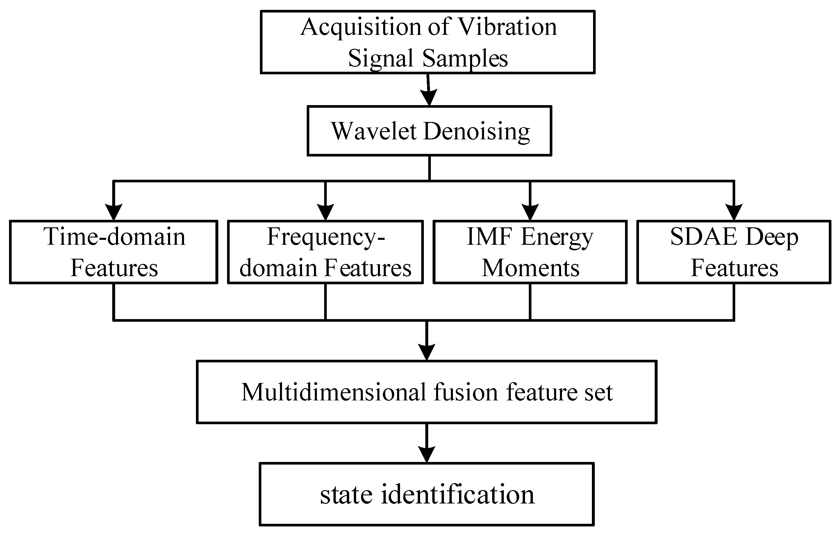
2. Integrating Multidimensional Information Features for State Recognition of Hydroelectric Units

2.1. IMF Energy Moment Feature Extraction Based on CEEMD

2.1.1. Complementary Ensemble Empirical Mode Decomposition

Empirical mode decomposition (EMD) is based on the distribution of extreme points in the signal itself, without the need for selecting basis functions. It has strong adaptability and a simple calculation process, but there are drawbacks such as endpoint effects and mode aliasing [15]. Ensemble empirical mode decomposition (EEMD) utilizes the uniform distribution of the white noise spectrum and the behavior of EMD filter banks to add normally distributed white noise to the analyzed signal for EMD decomposition, effectively suppressing the mode mixing caused by intermittent high-frequency components and other factors [16]. However, a certain number of ensemble averaging cannot completely eliminate white noise, resulting in poor signal decomposition completeness. Complementary empirical modal decomposition (CEEMD) adds positive and negative pairs of auxiliary white noise to the original signal, which can cancel each other out when averaging the ensembles, partially weakening the effect of residual noise on the decomposition effect. For the specific steps of the CEEMD processing signal, refer to the literature.

2.1.2. IMF Energy Moment

The IMFs generated by CEEMD decomposition are a series of narrowband components with different frequency components, and the characteristic differences of the IMF reflect the changes in the local details and frequency characteristics of the signal, which provide effective information for evaluating the operating status of the unit [17]. The IMF energy moment calculation method introduces the time factor on the basis of a traditional IMF energy analysis, which further embodies the distribution change in signal energy on the time scale and is suitable for the extraction of mechanical equipment fault features [18]. The feature extraction process based on IMF energy moments is as follows:

• Perform CEEMD processing on vibration signals to obtain n-order IMF components, and calculate the energy moments of each order of IMF component:

$$E_j=\sum _{i=1}^N(i·\Delta t){\left|c_j(i·\Delta t)\right|}^2,(j=1,2,3,\dots ,n)$$

(1)

In the formula, $i$ is the sampling number; $\Delta t$ is the sampling time interval; $T$ is the number of sampling points; $E_j$ is the j–th order IMF energy moment of the sample signal; and $c_j\left(i\right)$ is the amplitude of the j–th IMF component of the signal at the i–th discrete point.

2.

Calculate the total energy:

$$E={\displaystyle \sum _{j=1}^n{E}_j}$$

(2)

3.

Normalize the energy moments of the IMF components and establish the feature vector $T$:

$$E_j^{\prime }=E_j/E,(j=1,2,3,\dots ,n)$$

(3)

$$T=[E_1^{\prime },E_2^{\prime },E_3^{\prime },\dots ,E_n^{\prime }]$$

(4)

In the formula, $E_j^{\prime }$ represents the normalized value of the j–th order IMF energy moment of the sample.

2.2. Feature Extraction Based on Stacked Denoising Autoencoder

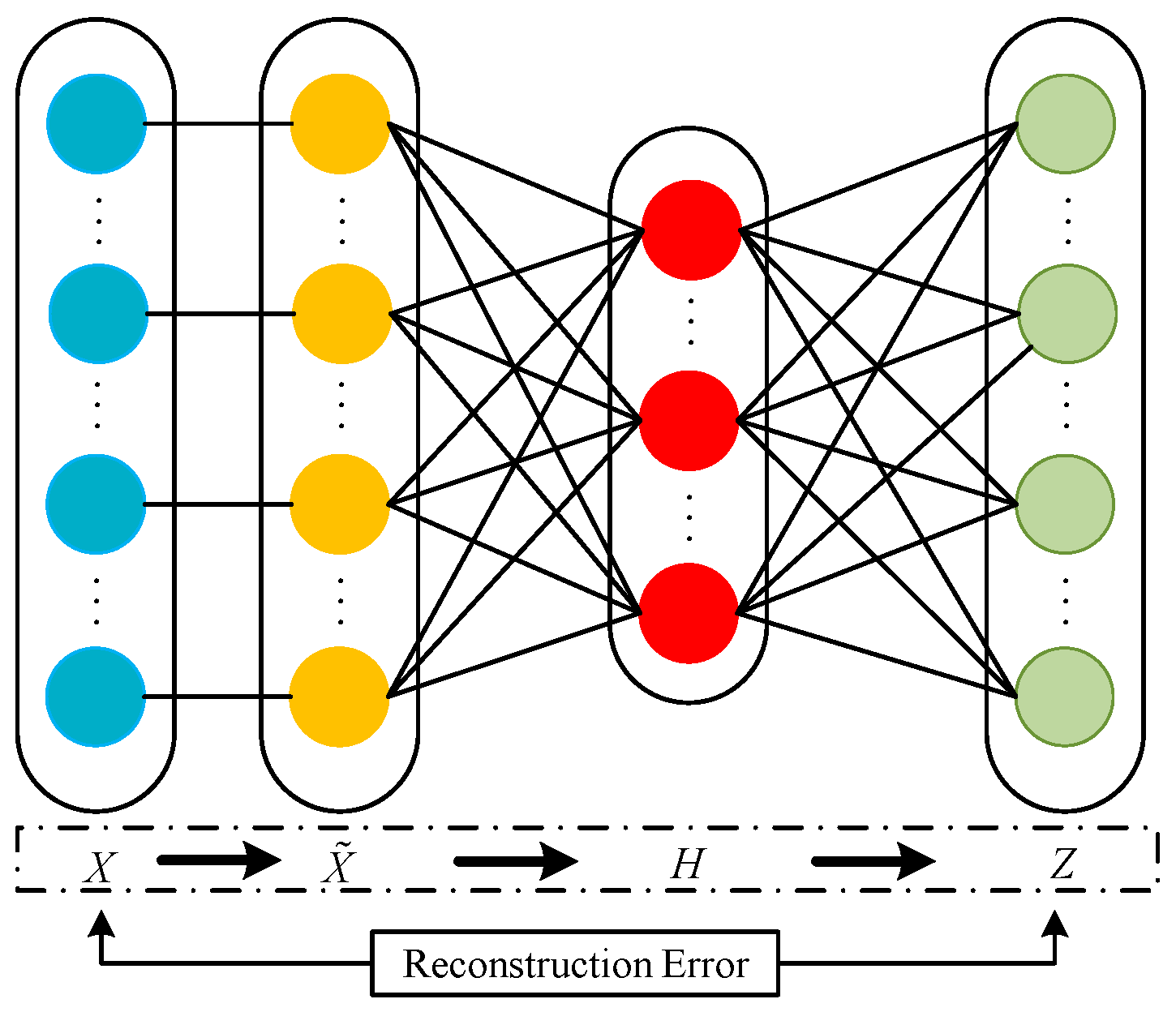
2.2.1. Autoencoder

An autoencoder (AE) is an unsupervised learning neural network that learns compact representations or features of data by minimizing the difference between input and reconstruction. It has been successfully applied in fields such as feature extraction, dimension reduction and fault diagnosis [19]. The typical network structure of an AE is shown in Figure 1. The encoding network includes an input layer and a hidden layer, which are responsible for extracting key features from the input data. The decoding network consists of a hidden layer and an output layer, which map the low–dimensional features generated by the encoder back to the original input space to achieve input data reconstruction.

In the AE algorithm, the encoding layer utilizes activation functions to nonlinearly map n–dimensional input data to an m–dimensional space, and in general, n > m, to achieve a low–dimensional representation of the input data. The decoding part restores the hidden feature information through weights and bias vectors, and forms a feature learning network in the way that the inter–layer nodes are fully connected and the intra-layer nodes are not connected, so that the output data are as close to the input data as possible. Namely,

$$H=f(X)=s(WX+b_1)$$

(5)

$$Y=g(H)=s(W\prime H+b_2)$$

(6)

In the formula, $X\in R^{n\times 1}$ is the input layer vector; $H\in R^{m\times 1}$ is the hidden layer vector; $Y\in R^{n\times 1}$ is the output layer vector; $W\in R^{m\times \mathrm{n}}$, $W\prime \in R^{n\times \mathrm{m}}$ represent the connection weights of the encoding network and the decoding network, respectively; $b_1\in R^{\mathrm{m}\times 1}$, $b_2\in R^{\mathrm{n}\times 1}$ represent the bias of the encoding network and the decoding network, respectively; and $s(x)$ is the activation function, and the sigmoid function $s(x)=1/\left(1+e^{-x}\right)$ is generally used.

During the training process of the standard AE model, a backpropagation algorithm is used to iteratively update the model weights and biases, to minimize the reconstruction error between the output data $Y$ and input data X, enabling the model to effectively capture key features of the input data. The mean square error loss function $L_1$ and cross-entropy loss function $L_2$ are two commonly used reconstruction error loss functions, and their calculation expressions are as follows:

$$L_1(X,Y)=\frac{1}{2}\sum _{i=1}^n{\left(y_i-x_i\right)}^2$$

(7)

$$L_2(X,Y)=-\sum _{i=1}^n\left[x_i\log \left(y_i\right)+\left(1-x_i\right)\log \left(1-y_i\right)\right]$$

(8)

For a set of unlabeled input samples $\left\{X_1,X_2,\dots ,X_s\right\}$, where $X_j=[x_{1j},x_{2j},\dots ,x_{nj}]$, the AE model reconstruction error loss functions are respectively,

$$L_1(X,Y)=\frac{1}{S}\sum _{j=1}^S\left(\frac{1}{2}\sum _{i=1}^n{\left(y_{ij}-x_{ij}\right)}^2\right)$$

(9)

$$L_2(X,Y)=-\frac{1}{S}\sum _{j=1}^S\left(\sum _{i=1}^n\left[x_{ij}\log \left(y_{ij}\right)+\left(1-x_{ij}\right)\log \left(1-y_{ij}\right)\right]\right)$$

(10)

In the formula, $S$ represents the total number of training samples, $n$ represents the dimension of each input sample, $x$ represents the i–th dimensional data of the j–th input sample, and $y$ represents the i–th dimensional data of the j–th reconstructed sample.

2.2.2. Denoising Autoencoder

A denoising autoencoder (DAE) is an effective extension of AE and has a stronger generalization ability [20]. A DAE consists of overcomplete and undercomplete hidden neuron layers; it corrupts the input data by adding random noise, extracts more stable hidden information from the noisy data, helps to solve the overfitting problem during the model-training process, and generates more robust feature representations when dealing with non-smooth signals, and its network structure is shown in Figure 2.

Given an input vector $X$, the DAE adds random noise to the input data through a random mapping transformation $\tilde{X}\sim q_D\left(\tilde{X}|X\right)$, resulting in the “contaminate” data $\tilde{X}$; $q_D$ is represented as binomial random hidden noise. Therefore, the encoding output H of the DAE and the reconstructed decoding output Z are:

$$H=f(X)=s(W\tilde{X}+b_1)$$

(11)

$$Z=g(H)=s(W\prime H+b_2)$$

(12)

During the training process, the mean square error function $L_1(X,Z)$ is used as the loss function to minimize the error between the reconstructed output and the original noise free input, in order to obtain the optimal model parameters. When the iteratively computed $L_1(X,Z)$ is small, it indicates that the denoising autoencoder model can effectively reconstruct the original data from noisy data. The encoded data can be used as a low-dimensional representation of the original signal and can be effectively used as signal features for equipment operation status analysis.

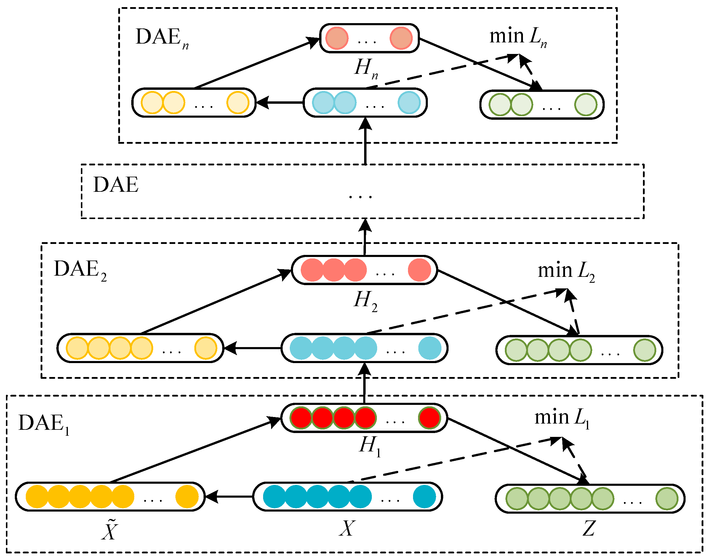
2.2.3. Construction of Stacked Noise Reduction Autoencoder Model

As a shallow network, the DAE mainly focuses on learning low-level feature representations of the input data. Its shallow structure may limit the model’s expressive ability when dealing with actual complex data, and it cannot extract deeper and essential features of the data. A Stacked Denoising Autoencoder (SDAE) is formed by stacking multiple DAEs in sequence, which can learn and extract abstract features of data layer by layer and which has a strong deep nonlinear mapping ability [21].

The SDAE network structure is shown in Figure 3. During the greedy layer–by–layer training process, each DAE is independently trained in a bottom–up order. The lower-level DAE uses the hidden representation of the upper-level trained DAE as pure input, and is trained layer by layer until the highest hidden layer outputs the deepest high–order features of the original input signal. The greedy layer–by–layer training method can reduce the parameter optimization space and improve deep learning ability and model generalization ability [22].

2.3. Hydropower Unit State Recognition Method Based on Multidimensional Information Fusion Features

In response to the problem that it is difficult to effectively measure the correspondence between a single feature indicator and the operating status of the unit equipment under various factors such as hydraulic, mechanical and electromagnetic interference, this paper extracts the IMF energy moments and SDAE depth features of the vibration signals of the hydropower unit based on the time–frequency analysis principle and deep learning technology, and combines these with the typical time–domain features and the frequency–domain features as shown in

Table 1. Time–domain and frequency–domain characteristics.

Feature Name	Time–Domain Feature	Feature Name	Frequency–Domain Feature
standard deviation	$T_1=\sqrt{\frac{1}{N}{\displaystyle \sum _{n=1}^N{(x(n)-\overline{T})}^2}}$	mean frequency amplitude	$F_1=\frac{1}{K}{\displaystyle \sum _{k=1}^{K}s(k)}$
peak-to-peak value	$T_2=\max \left\{\left|x(i)\right|\right\}-\min \left\{\left|x(i)\right|\right\}$	frequency centroid value	$F_2=\frac{{\displaystyle \sum _{k=1}^K{f}_{k}s(k)}}{{\displaystyle \sum _{k=1}^{K}s(k)}}$
kurtosis	$T_3=\frac{1}{N}{\displaystyle \sum _{i=1}^N\frac{{(x(n)-\overline{T})}^4}{T_1^4}}$	frequency standard deviation	$F_3=\sqrt{\frac{{\displaystyle \sum _{k=1}^K{\left(f_k-F_2\right)}^{2}s(k)}}{{\displaystyle \sum _{k=1}^{K}s(k)}}}$

, to explore the information of data from multiple angles, to construct a multidimensional fusion feature vector of the vibration signals of the hydropower unit. The structure of the multidimensional fusion feature vector of the vibration signal of the hydropower unit is shown in Figure 4. $[F{H}_1,F{H}_2,\dots ,F{H}_n]$ represents the SDAE deep feature vector.

The fault identification process for hydroelectric units based on the multidimensional fusion features of vibration signals is shown in Figure 5.

• Based on the wavelet threshold denoising method, the vibration signal of hydroelectric units is preprocessed. The “db8” wavelet function is selected with three decomposition layers, and the number of decomposition layers is selected as three layers.
• Extract the time–domain features, frequency–domain features, IMF energy moments and SDAE deep features from the noise-canceled signal to construct a multidimensional fusion feature vector of the vibration signal.
• Learn and diagnose pattern categories based on the extracted multidimensional fusion feature vectors.

3. Verification and Analysis

To verify the practical application effect of the multidimensional information fusion feature extraction method in the field of hydropower, the No. 3 axial flow paddle unit of the SK power station in China is analyzed as an example. The unit vibrated strongly during operation in August 2015, and significant noise was generated at positions such as the upper frame and volute. It was later discovered that the middle ring steel plate of the unit runner chamber fell off, and the blade skirt was seriously damaged. The fault location is shown in Figure 6.

The speed of the No. 3 unit is 107.1 r/min, and the sampling frequency is 458 Hz. Obtain the axial vibration data before and after the failure in the same operating condition interval to analyze and classify its operating state into two states: normal and failure. Use 100 sets of normal sample data and 100 sets of fault samples each, with a sampling length of 4096. The original signals in each state are subjected to decentralization and noise reduction processing, and the waveforms are shown in Figure 7. There are certain differences in amplitude and waveform shape between the two signals.

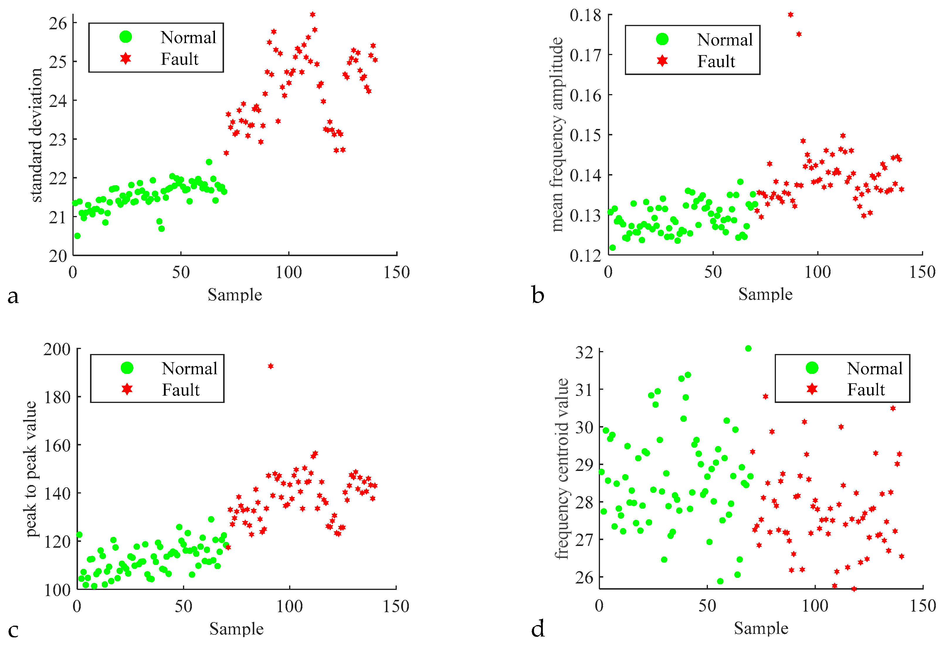
3.1. Time–Domain and Frequency–Domain Feature Extraction

Extract the time–domain and frequency–domain characteristics of the measured axial vibration signals of the SK unit. The time and frequency features of the vibration signal samples in different states are shown in

Table 2. Time–domain and frequency–domain features of measured axial vibration signals.

State	Sample ID	T1	T2	T3	F1	F2	F3
Normal	90	22.131	117.754	2.564	0.132	28.900	34.700
Fault	190	26.582	155.945	2.871	0.152	28.490	31.775

. From the comparison of single–sample data, there are differences in the separability of the samples in different states under different time– and frequency–domain characteristics. For example, the peak–to–peak value of the vibration signals in normal states is significantly smaller than the corresponding value in fault states, while the mean frequency amplitude difference of the samples in different states is relatively small.

To further compare the discriminative effects of the SK power plant unit states in different time and frequency domains, we will plot the distributions of the time–domain and frequency–domain features of equal quantities of normal and faulty sample signals. This visualization aims to intuitively showcase differences in feature values between different samples. As depicted in Figure 8, the standard deviation of all the normal samples is consistently lower than that of the fault samples, showcasing a pronounced distinction between the two datasets. In the case of peak–to–peak value, kurtosis and mean frequency amplitude, the values of fault samples are generally higher than those of normal samples. However, there exists a local overlap in the distribution of features under different states, such as the mean frequency amplitude ranging from 0.13 to 0.14. In contrast, the similarity of normal and fault samples is the highest and the separability is the worst under the frequency barycenter value and frequency standard deviation. It can be seen that solely relying on traditional time–domain or frequency–domain features to identify the state of the unit leads to significant inaccuracies and randomness. It is necessary to extract other effective features to achieve a more comprehensive description of the unit’s state.

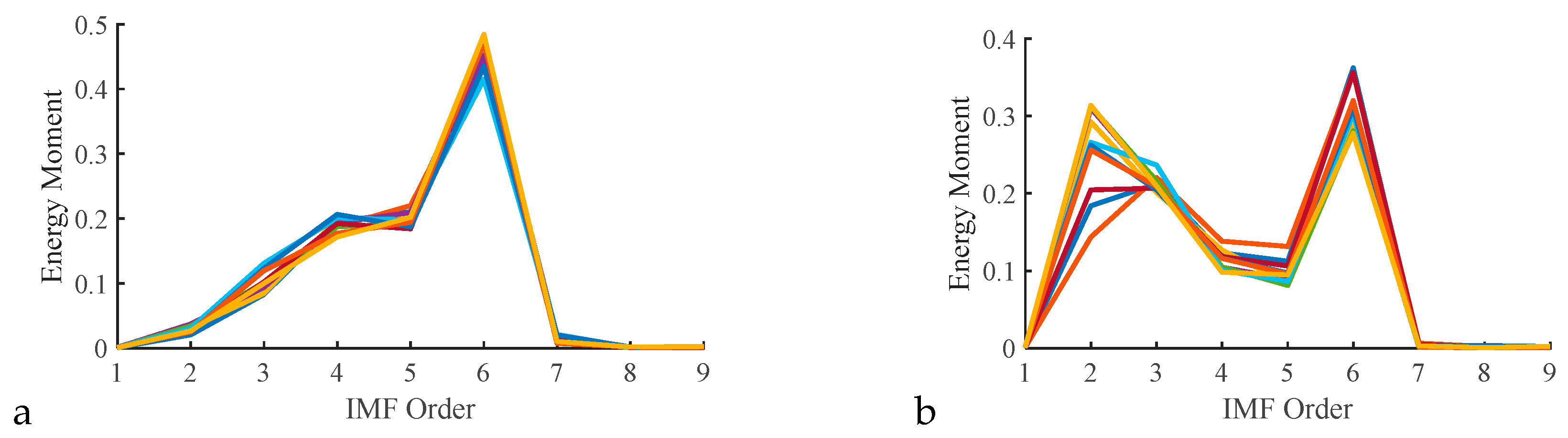
3.2. IMF Energy Moment Feature Extraction

CEEMD was used to decompose the denoised vibration signal. The decomposition results of vibration signals under normal and fault conditions are shown in Figure 9.

CEEMD was used to decompose the denoised vibration signal. The decomposition results of vibration signals under normal and fault conditions are shown in Figure 10.

3.3. SDAE Feature Extraction

Construct a Stacked Denoising Autoencoder (SDAE) model for feature extraction from vibration signals, with the hidden layer parameters set as 2000–1000–400–50. Thirty sets of normal samples and thirty sets of faulty samples were randomly selected. T–SNE was employed to visualize the dimensionality reduction of the SDAE feature data obtained from the actual vibration signals of hydroelectric units. The results, depicted in Figure 11, show that normal and faulty samples are clustered separately, with a distinct separation between different states. This suggests that the SDAE can automatically learn and extract latent features that effectively represent the state of the unit, thereby aiding in reducing data redundancy.

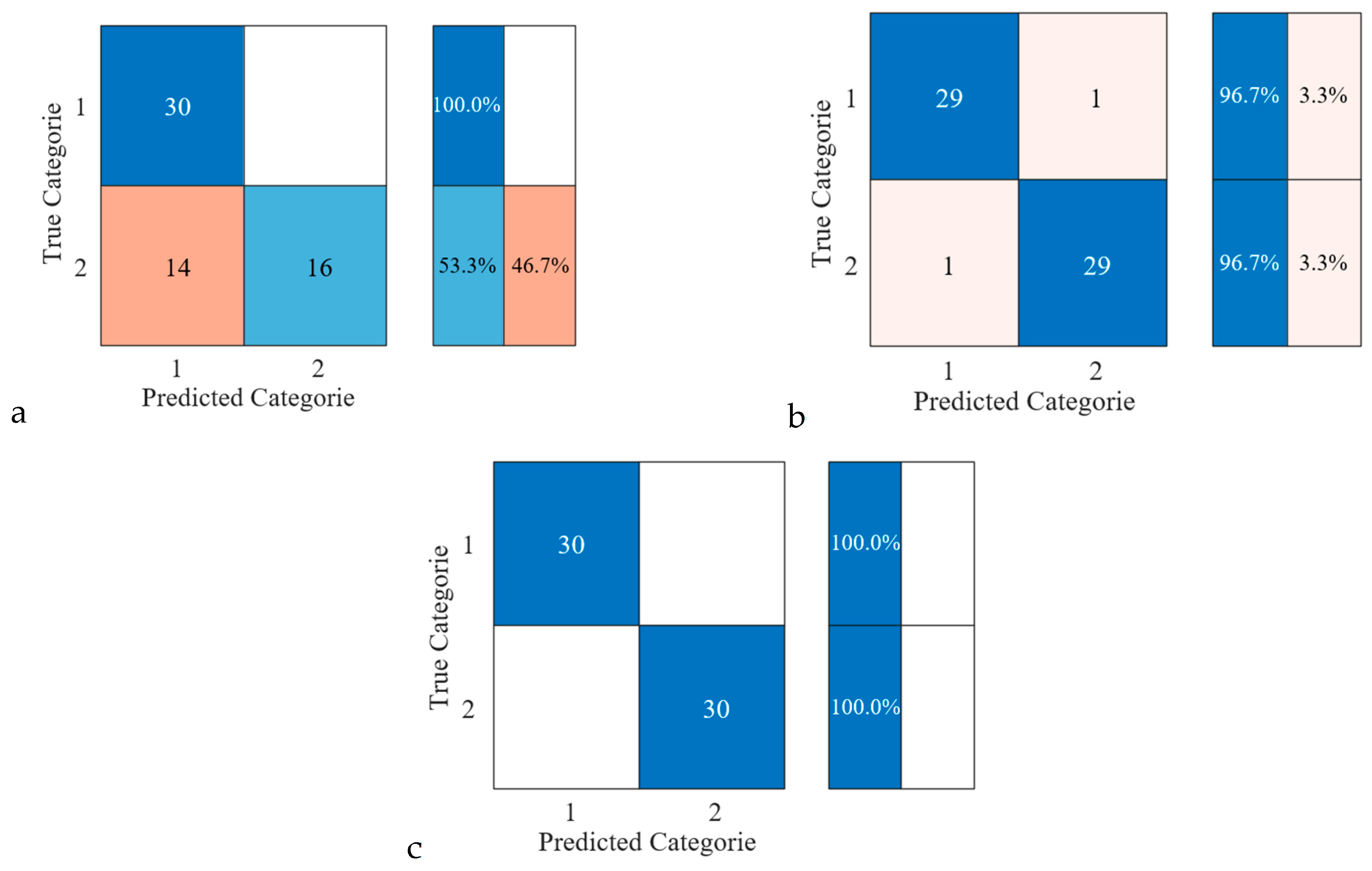
3.4. Multidimensional Information Fusion Feature Effectiveness Analysis

Construct a fused feature matrix by integrating four types of features extracted from vibration signals, and employ the backpropagation neural network (BPNN) for pattern recognition. The training set and test set are divided into a 7:3 ratio. The recognition performance is illustrated in Figure 12, where labels 1 and 2 represent the categories of normal and fault states, respectively. The BPNN based on traditional time and frequency features achieves a recognition rate of 100% for normal state signals but tends to misclassify fault samples as normal states, resulting in the poorest overall recognition performance. Utilizing the multidimensional fused features proposed in this paper as inputs, the BPNN achieves the complete recognition of both normal and fault samples, indicating that the multidimensional fusion feature extraction supplemented by IMF energy moments and SDAE features further improves the accuracy of the BPNN’s equipment state recognition.

The specific recognition results of the BPNN based on different feature types are shown in Figure 13. With multidimensional information fusion feature vectors as input, BPNN has a recognition accuracy of 100% for both normal and fault samples of the unit, achieving an effective differentiation of different state samples. The overall sample recognition accuracy of the BPNN based on traditional time–domain and frequency–domain features is 76.67%, while that based on SDAE features is 96.67%. The device state recognition accuracy of the BPNN based on the proposed multidimensional information fusion feature matrix has been improved by 23.33% and 3.33%, respectively. This indicates that the combination of time–domain and frequency–domain features with IMF energy moment features and SDAE self-extracted features effectively enhances the effectiveness and practicality of the multidimensional information matrix. It achieves the multidimensional complementarity of feature attributes, contributing to an increased accuracy in state recognition.

In order to further analyze the feasibility and effectiveness of the feature extraction method, a Support Vector Machine (SVM) was used to identify the feature data of Unit 3 of SK Power Station under different states. A total of 70 groups of signal samples were randomly selected for training under each state, and the remaining 30 groups of samples were used as test sets for verification. The status recognition effect is shown in Figure 14. For the signal multidimensional information fusion feature matrix under normal and fault conditions, the SVM’s recognition accuracy is 83.3% and 100%, respectively, indicating that after the extraction of multidimensional information fusion features, different samples have a certain separability. Combined with the method proposed in this chapter, the overall signal state recognition accuracy of the SVM is 91.67%, which is about 5% and 1.67% higher than that of the SVM based on traditional time– and frequency–domain features and SDAE features, respectively, achieving a more accurate recognition effect, which further indicates that the proposed fusion feature matrix has a good signal characterization ability. This is helpful for improving the accuracy of fault identification.

4. Discussion

The example of the vibration signal feature extraction of the No. 3 rotating propeller unit of the SK Power Station in China shows that the original signal presents a relatively obvious nonlinear shape. The time–domain and frequency–domain characteristics can represent the distribution of the signal in the time domain and frequency domain, but they are not enough to fully reflect the operation of and dynamic changes in the equipment. The IMF energy moment of the vibration signal can effectively quantify the difference in IMF of different orders between different states of the unit and reflect the distribution of signal energy on the time scale. SDAE has a strong nonlinear representation ability and can learn the deep features of complex fault data adaptively. The multidimensional fusion feature vector of the vibration signals of hydropower units is constructed by combining the time–domain features, frequency–domain features, IMF energy moment and SDAE features, and a different classifier is used for state recognition. The comparison experiment results show that the recognition accuracy of the BP neural network and support vector machine has been effectively improved based on the features extracted by this method. It is verified that the proposed fusion feature matrix has a better signal characterization ability.

5. Conclusions

To address the limitations of traditional time–domain or frequency–domain features in fully capturing dynamic abrupt behaviors in the non–stationary vibration signals of equipment anomalies, this paper proposes a method for constructing a multidimensional fused feature matrix for hydroelectric turbine vibration signals by integrating traditional time–domain and frequency–domain features, IMF energy moments and SDAE deep features. The following conclusions are drawn:

• Combining the advantages of CEEMD’s non–smooth signal-processing capability and anti–modal aliasing and the reduction of the influence of residual noise, extract the IMF components of the signal and compute the energy moment features. This effectively supplements the multidimensional feature matrix for a more comprehensive characterization of vibration signals.
• Constructing an SDAE model to adaptively mine robust deep features from vibration signal samples, and using t–SNE to reduce dimensionality and visualize SDAE feature data, it is shown that the self-extracted features of the SDAE can effectively represent different states of equipment, breaking through the limitations of traditional feature extraction relying on expert experience and prior knowledge and effectively improving the generalization ability of model feature learning.
• According to the proposed multidimensional information fusion feature matrix, the BPNN equipment state recognition accuracy is 100%, which is 23.33% and 3.33% higher than the BPNN recognition accuracy based on traditional time, frequency and SDAE features, respectively. By comparing the effectiveness of the BPNN and SVM in identifying unit state types based on traditional time–domain and frequency–domain features, it is proven that the multidimensional fusion feature matrix constructed by supplementing IMF energy moments and SDAE deep features can more comprehensively mine signal information, achieve the multidimensional complementarity of feature attributes, help to accurately distinguish equipment state types and provide support for subsequent state recognition and trend prediction.
• With the development of sensor technology and the Internet of Things, it becomes more convenient to obtain multi-mode data. In the follow–up research, we can try to integrate various signals such as vibration, acoustics and temperature to comprehensively capture the operating state of the equipment and improve the accuracy and robustness of fault diagnosis.

References

1. Kumar, K.; Saini, R. A review on operation and maintenance of hydropower plants. Sustain. Energy Technol. Assess. 2022, 49, 101704. [Google Scholar] [CrossRef]
2. Li, X.; Xu, Z.; Wang, Y. PSO–MCKD–MFFResnet based fault diagnosis algorithm for hydropower units. Math. Biosci. Eng. 2023, 20, 14117–14135. [Google Scholar]
3. Jia, L.; Zeng, Y.; Liu, X.; Huang, W.; Xiao, W. Testing and Numerical Analysis of Abnormal Pressure Pulsations in Francis Turbines. Energies 2024, 17, 237. [Google Scholar]
4. Siddique, M.F.; Ahmad, Z.; Ullah, N.; Kim, J. A Hybrid Deep Learning Approach: Integrating Short–Time Fourier Transform and Continuous Wavelet Transform for Improved Pipeline Leak Detection. Sensors 2023, 23, 8079. [Google Scholar] [PubMed]
5. Syed, S.H.; Muralidharan, V. Feature extraction using Discrete Wavelet Transform for fault classification of planetary gearbox–A comparative study. Appl. Acoust. 2022, 188, 108572. [Google Scholar]
6. Sarangi, S.; Biswal, C.; Sahu, B.K.; Samanta, I.S.; Rout, P.K. Fault detection technique using time–varying filter–EMD and differential–CUSUM for LVDC microgrid system. Electr. Power Syst. Res. 2023, 219, 109254. [Google Scholar]
7. Zhang, Q.; Deng, L. An intelligent fault diagnosis method of rolling bearings based on short–time Fourier transform and convolutional neural network. J. Fail. Anal. Prev. 2023, 23, 795–811. [Google Scholar] [CrossRef]
8. Lu, Y.; Li, P. A Novel Fault Diagnosis Method for Motor Bearing Based on DTCWT and AFSO–KELM. Shock Vib. 2021, 2021, 2108457. [Google Scholar] [CrossRef]
9. Bin, G.; Gao, J.; Li, X.; Dhillon, B. Early fault diagnosis of rotating machinery based on wavelet packets—Empirical mode decomposition feature extraction and neural network. Mech. Syst. Signal Process. 2012, 27, 696–711. [Google Scholar] [CrossRef]
10. Sahu, P.K.; Rai, R.N. Fault diagnosis of rolling bearing based on an improved denoising technique using complete ensemble empirical mode decomposition and adaptive thresholding method. J. Vib. Eng. Technol. 2023, 11, 513–535. [Google Scholar] [CrossRef]
11. Hou, Y.; Ma, J.; Wang, J.; Li, T.; Chen, Z. Enhanced generative adversarial networks for bearing imbalanced fault diagnosis of rotating machinery. Appl. Intell. 2023, 53, 25201–25215. [Google Scholar] [CrossRef]
12. Dao, F.; Zeng, Y.; Qian, J. Fault diagnosis of hydro-turbine via the incorporation of bayesian algorithm optimized CNN–LSTM neural network. Energy 2024, 290, 130326. [Google Scholar] [CrossRef]
13. Wu, X.; Zhang, Y.; Cheng, C.; Peng, Z. A hybrid classification autoencoder for semi-supervised fault diagnosis in rotating ma-chinery. Mech. Syst. Signal Process. 2021, 149, 107327. [Google Scholar] [CrossRef]
14. Almuqren, L.; Aljameel, S.S.; Alqahtani, H.; Alotaibi, S.S.; Hamza, M.A.; Salama, A.S. A White Shark Equilibrium Optimizer with a Hybrid Deep–Learning–Based Cybersecurity Solution for a Smart City Environment. Sensors 2023, 23, 7370. [Google Scholar] [CrossRef] [PubMed]
15. Kumar, A.; Berrouche, Y.; Zimroz, R.; Vashishtha, G.; Chauhan, S.; Gandhi, C.; Tang, H.; Xiang, J. Non−parametric Ensemble Empirical Mode Decomposition for extracting weak features to identify bearing defects. Measurement 2023, 211, 112615. [Google Scholar] [CrossRef]
16. Lobato, T.H.G.; da Silva, R.R.; da Costa, E.S.; Mesquita, A.L.A. An integrated approach to rotating machinery fault diagnosis using, EEMD, SVM, and augmented data. J. Vib. Eng. Technol. 2020, 8, 403–408. [Google Scholar] [CrossRef]
17. Bendjama, H. Feature extraction based on vibration signal decomposition for fault diagnosis of rolling bearings. Int. J. Adv. Manuf. Technol. 2024, 130, 821–836. [Google Scholar] [CrossRef]
18. Pang, Y.; Gao, J.-W. Fault Diagnosis Method of Rolling Bearings Based on ICEEMDAN Energy Moment and HHO–KLEM. Noise Vib. Control 2023, 43, 142–148. [Google Scholar]
19. Jang, J.-G.; Noh, C.-M.; Kim, S.-S.; Shin, S.-C.; Lee, S.-S.; Lee, J.-C. Vibration data feature extraction and deep learning–based preprocessing method for highly accurate motor fault diagnosis. J. Comput. Des. Eng. 2023, 10, 204–220. [Google Scholar] [CrossRef]
20. Neelakandan, S.; Reddy, N.V.R.; Ghfar, A.A.; Pandey, S.; Kiran, S.; Arasu, P.T. Internet of things with nanomaterials–based predictive model for wastewater treatment using stacked sparse denoising auto–encoder. Water Reuse 2023, 13, 233–249. [Google Scholar] [CrossRef]
21. Jorkesh, S.; Gholaminejad, A.; Poshtan, J. Induction motors fault diagnosis using a stacked sparse auto–encoder deep neural network. Proc. Inst. Mech. Eng. Part I J. Syst. Control Eng. 2023, 237, 359–369. [Google Scholar] [CrossRef]
22. Key, S.; Ko, C.-S.; Song, K.-J.; Nam, S.-R. Fast detection of current transformer saturation using stacked denoising autoencoders. Energies 2023, 16, 1528. [Google Scholar] [CrossRef]
Figure 1. Structure diagram of AE.
Water 16 01956 g001
Figure 2. Network structure of DAE model.
Water 16 01956 g002
Figure 3. SDAE network architecture diagram.
Water 16 01956 g003
Figure 4. Multidimensional fused feature vector.
Water 16 01956 g004
Figure 5. Fault diagnosis of hydroelectric unit based on fused features.
Water 16 01956 g005
Figure 6. Detachment of the steel plate in the turbine room of Unit 3.
Water 16 01956 g006
Figure 7. Actual measured axial vibration signals of Unit SK. (a) Normal state, and (b) Fault state.
Water 16 01956 g007
Figure 8. Distribution of time–domain and frequency–domain features of vibration signals. (a) standard deviation, and (b) mean frequency amplitude, and (c) peak−to−peak value, and (d) frequency centroid value, and (e) kurtosis, and (f) frequency standard deviation.
Water 16 01956 g008aWater 16 01956 g008b
Figure 9. Decomposed results of vibration signals from Unit SK. (a) normal state, and (b) fault state.
Water 16 01956 g009
Figure 10. IMF energy moment curves of signals under different states. (a) IMF energy moment curve of signal in normal state, (b) IMF energy moment curve of signal in fault state.
Water 16 01956 g010
Figure 11. Visualization result of SDAE characteristics of SK vibration signals under different states. (a) SDAE deep features, and (b) T–SNE visualization result.
Water 16 01956 g011
Figure 12. The recognition effect of hydroelectric unit states based on different features. (a) Recognition based on traditional time–domain and frequency–domain feature, and (b) Recognition based on SDAE features, and (c) Recognition based on multidimensional information fusion features.
Water 16 01956 g012
Figure 13. Confusion matrix for BPNN state recognition based on different features. (a) Confusion matrix plot for recognition based on traditional time and frequency features, and (b) Confusion matrix plot for recognition based on SDAE features, and (c) Confusion matrix plot for recognition based on multidimensional fused features.
Water 16 01956 g013
Figure 14. Confusion matrix for SVM state recognition based on different features. (a) Confusion matrix plot for recognition based on traditional time and frequency features, and (b) Confusion matrix plot for recognition based on SDAE features, and (c) Confusion matrix plot for recognition based on multidimensional fused features.
Water 16 01956 g014