
Limnological Characteristics and Relationships with Primary Productivity in Two High Andean Hydroelectric Reservoirs in Ecuador
 , , , , and
Abstract
:1. Introduction
2. Materials and Methods
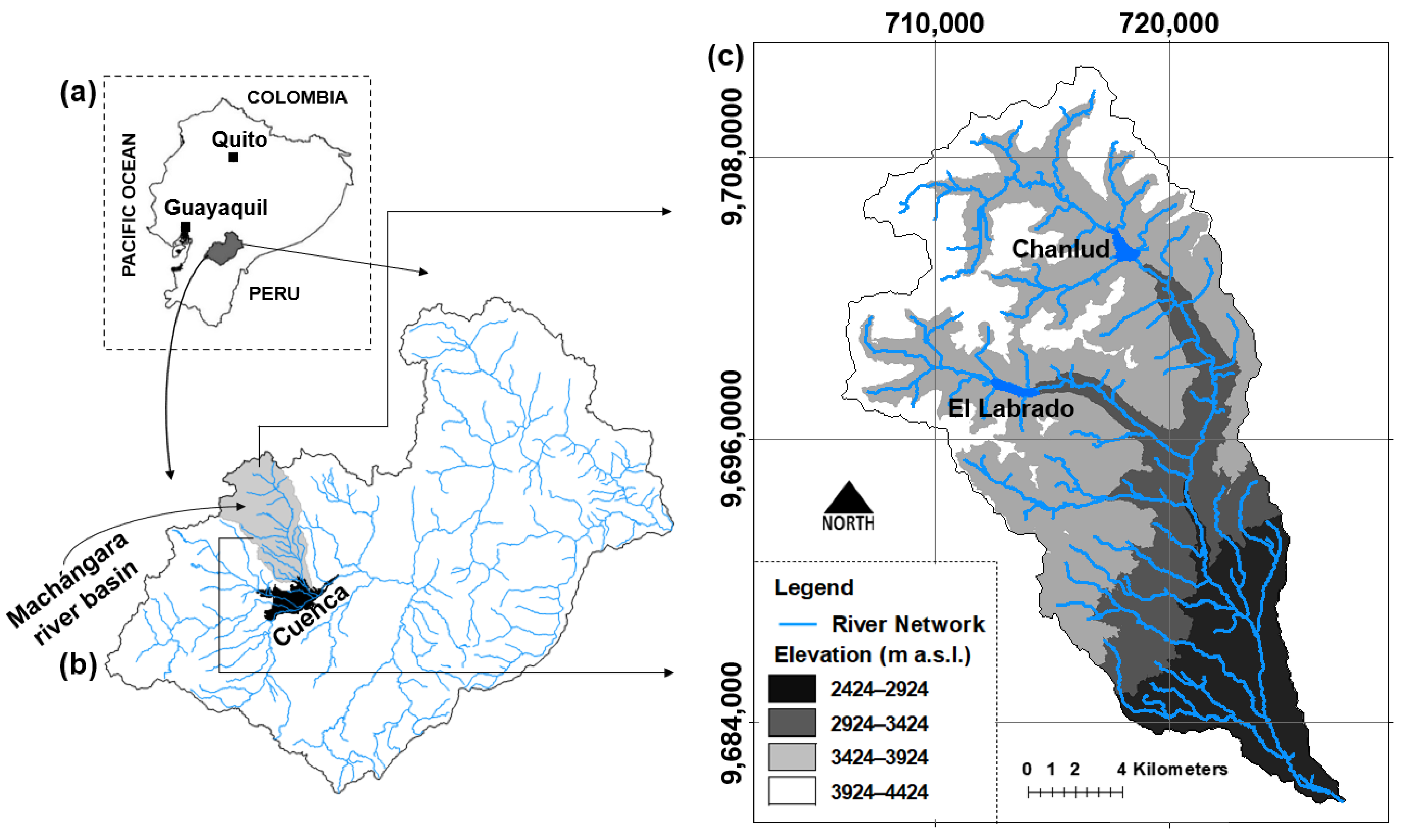
2.1. Study Area
2.2. Sampling Design
2.3. Data Analysis
2.3.1. Principal Component Analysis (PCA)
2.3.2. Multiple Linear Regression Analysis (MLRA)
3. Results
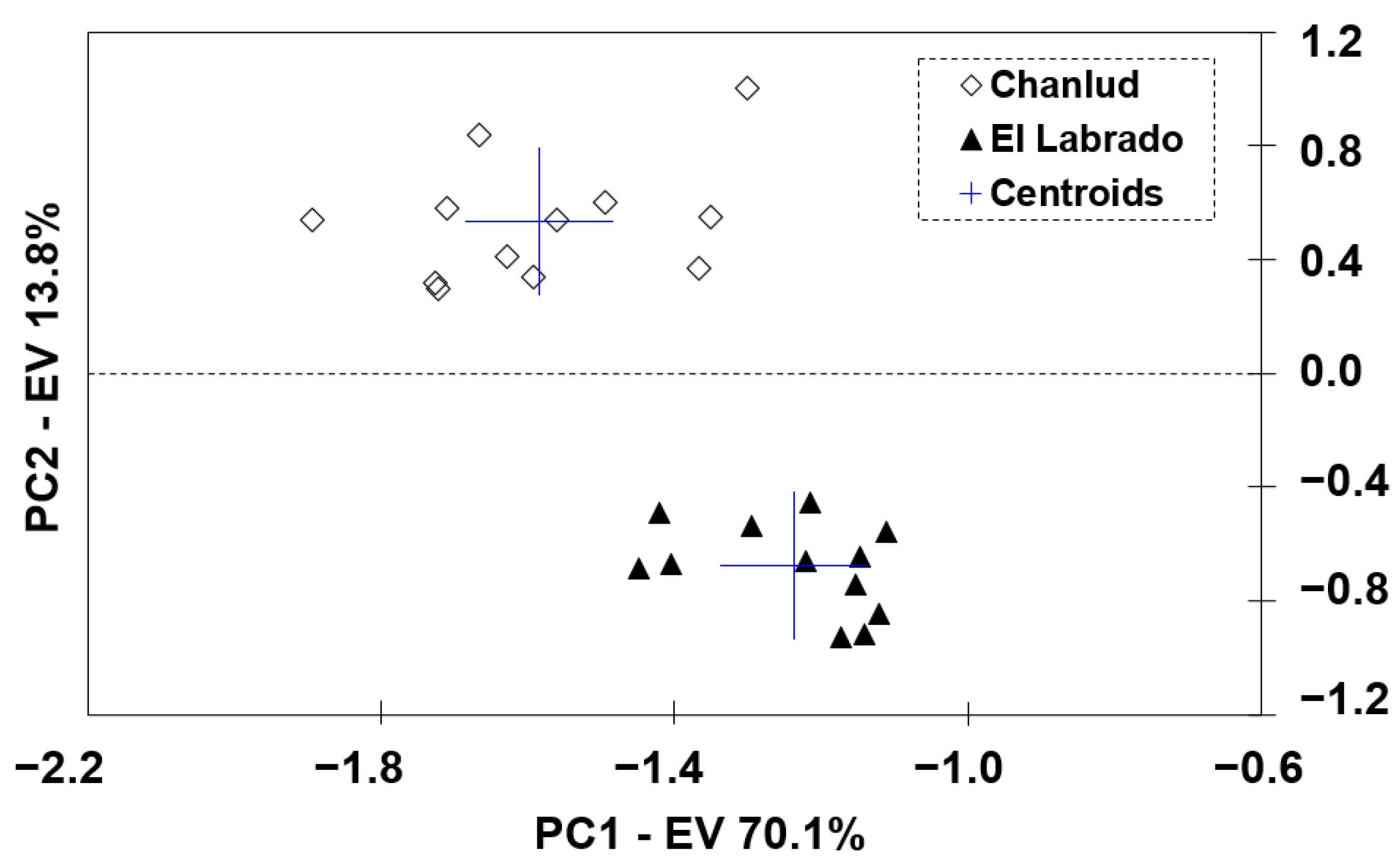
3.1. Principal Component Analysis (PCA)
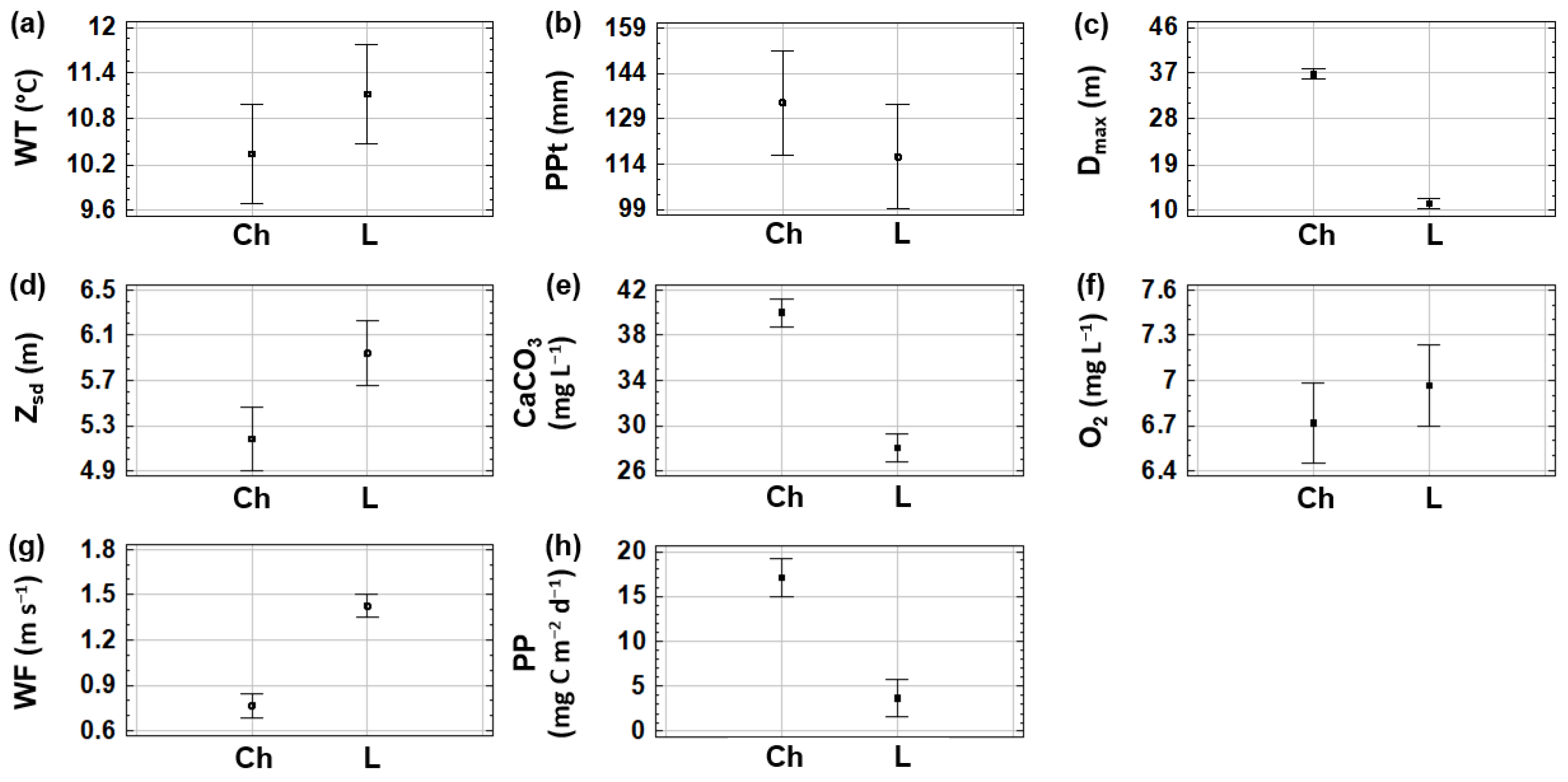
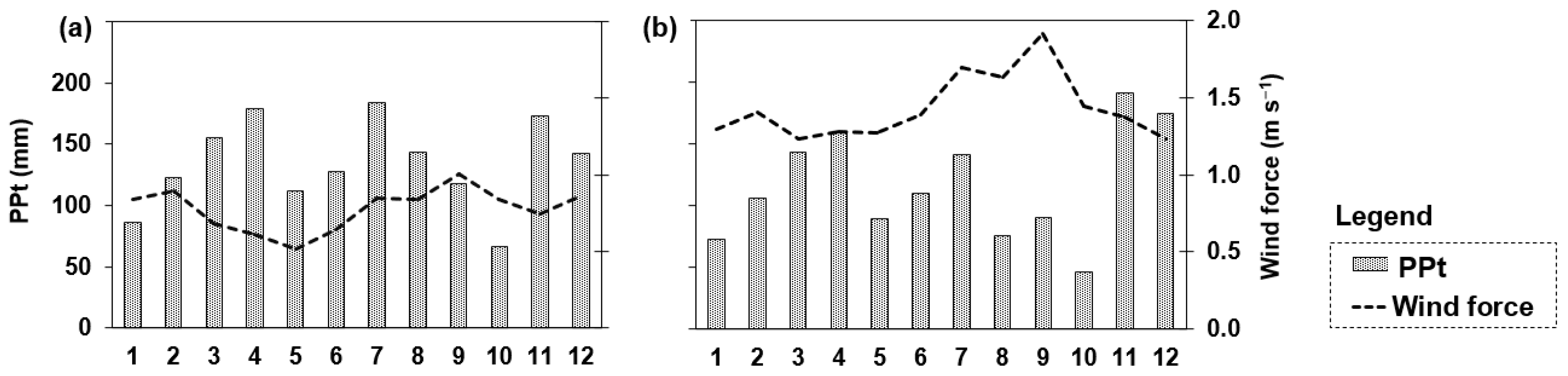
Analysis of the Variables Identified by PCA as Informative to the Studied Reservoirs
3.2. Multiple Linear Regression Analysis (MLRA)
4. Discussion
5. Conclusions
Author Contributions
Funding
Data Availability Statement
Acknowledgments
Conflicts of Interest
References
- Rodgher, S.; Espíndola, E.L.; Rocha, O.; Fracácio, R.; Pereira, R.H.; Rodrigues, M.H. Limnological and ecotoxicological studies in the cascade of reservoirs in the Tietê River (São Paulo, Brazil). Braz. J. Biol. 2005, 65, 697–710. [Google Scholar] [CrossRef] [PubMed]
- Zarfl, C.; Lumsdon, A.E.; Berlekamp, J.; Tydecks, L.; Tockner, K. A global boom in hydropower dam construction. Aquat. Sci. 2015, 77, 161–170. [Google Scholar] [CrossRef]
- Bredenhand, E.; Samways, M.J. Impact of a dam on benthic macroinvertebrates in a small river in a biodiversity hotspot: Cape Floristic Region, South Africa. J. Insect Conserv. 2009, 13, 297–307. [Google Scholar] [CrossRef]
- Nguyen, T.H.T.; Everaert, G.; Boets, P.; Forio, M.A.E.; Bennetsen, E.; Volk, M.; Hoang, T.H.T.; Goethals, P.L.M. Modelling tools to analyze and assess the ecological impact of hydropower dams. Water 2018, 10, 259. [Google Scholar] [CrossRef]
- Margalef, R. Limnología; Omega: Barcelona, Spain, 1983. [Google Scholar]
- Bengtsson, L.; Herschy, R.W.; Fairbridge, R.W. Encyclopedia of Lakes and Reservoirs; Springer: Dordrecht, The Netherland, 2012. [Google Scholar]
- Simões, N.R.; Nunes, A.H.; Dias, J.D.; Lansac-Tôha, F.A.; Velho, L.F.M.; Bonecker, C.C. Impact of reservoirs on zooplankton diversity and implications for the conservation of natural aquatic environments. Hydrobiologia 2015, 758, 3–17. [Google Scholar] [CrossRef]
- Song, C.; Gardner, K.H.; Klein, S.J.W.; Souza, S.P.; Mo, W. Cradle-to-grave greenhouse gas emissions from dams in the United States of America. Renew. Sustain. Energy Rev. 2018, 90, 945–956. [Google Scholar] [CrossRef]
- Dodds, W.K.; Whiles, M.R. Freshwater Ecology; Academic Press: Cambridge, MA, USA, 2019. [Google Scholar]
- Páez, R.; Ruiz, G.; Márquez, R.; Soto, L.M.; Montiel, M.; López, C. Limnological studies on a shallow reservoir in Western Venezuela (Tulé Reservoir). Limnologica 2001, 31, 139–145. [Google Scholar] [CrossRef]
- Silva, R.F.C.M.; de Almeida, T.; Cicerelli, R.E.; Gomes, L.N.L. A spatiotemporal analysis of the physicochemical parameters after the operation of the Corumbá IV reservoir (Midwest Brazil) to support better management decision. Environ. Monit. Assess. 2021, 193, 247. [Google Scholar] [CrossRef] [PubMed]
- Williamson, C.E.; Saros, J.E.; Vincent, W.F.; Smol, J.P. Lakes and reservoirs as sentinels, integrators, and regulators of climate change. Limnol. Oceanogr. 2009, 54, 2273–2282. [Google Scholar] [CrossRef]
- Soares, M.C.S.; Marinho, M.M.; Huszar, V.L.M.; Branco, C.W.C.; Azevedo, S.M.F.O. The effects of water retention time and watershed features on the limnology of two tropical reservoirs in Brazil. Lakes Reserv. Res. Manag. 2008, 13, 257–269. [Google Scholar] [CrossRef]
- Gansser, A. Facts and theories on the andes. J. Geol. Soc. 1973, 129, 93–131. [Google Scholar] [CrossRef]
- Michelutti, N.; Tapia, P.M.; Labaj, A.L.; Grooms, C.; Wang, X.; Smol, J.P. A limnological assessment of the diverse waterscape in the Cordillera Vilcanota, Peruvian Andes. Inland Waters 2019, 9, 395–407. [Google Scholar] [CrossRef]
- Aguilera, X.; Declerck, S.; De Meester, L.; Maldonado, M.; Ollevier, F. Tropical high Andes lakes: A limnological survey and an assessment of exotic rainbow trout (Oncorhynchus mykiss). Limnologica 2006, 36, 258–268. [Google Scholar] [CrossRef]
- Cabrol, N.A.; Grin, E.A.; Chong, G.; Minkley, E.; Hock, A.N.; Yu, Y.; Bebout, L.; Fleming, E.; Häder, D.P.; Demergasso, C.; et al. The High-Lakes Project. J. Geophys. Res. Biogeosci. 2009, 114, G00D06. [Google Scholar] [CrossRef]
- Fortner, S.K.; Mark, B.G.; McKenzie, J.M.; Bury, J.; Trierweiler, A.; Baraer, M.; Burns, P.J.; Munk, L. Elevated stream trace and minor element concentrations in the foreland of receding tropical glaciers. Appl. Geochem. 2011, 26, 1792–1801. [Google Scholar] [CrossRef]
- Benito, X.; Fritz, S.C.; Steinitz-Kannan, M.; Tapia, P.M.; Kelly, M.A.; Lowell, T.V. Geo-climatic factors drive diatom community distribution in tropical South American freshwaters. J. Ecol. 2018, 106, 1660–1672. [Google Scholar] [CrossRef]
- Marín-Ramírez, A.; Gómez-Giraldo, A.; Román-Botero, R. Variación estacional de la temperatura media y los flujos advectivos y atmosféricos de calor en un embalse tropical andino. Rev. Acad. Colomb. Cienc. Exactas Físicas Nat. 2020, 44, 360–375. [Google Scholar] [CrossRef]
- Villabona-González, S.L.; Benjumea-Hoyos, C.A.; Gutiérrez-Monsalve, J.A.; López-Muñoz, M.T.; González, E.J. Main physicochemical and biological variables in the trophic state of five Colombian Andean reservoirs. Rev. Acad. Colomb. Cienc. Exactas Físicas Nat. 2020, 44, 344–359. [Google Scholar]
- Tundisi, J.G.; Matsumura-Tundisi, T.; Calijuri, M.C. Limnology and management of reservoirs in Brazil. Comp. Reserv. Limnol. Water Qual. Manag. 1993, 1000, 25–55. [Google Scholar]
- Tundisi, J.G.; Matsumura-Tundisi, T. Integration of research and management in optimizing multiple uses of reservoirs: The experience in South America and Brazilian case studies. Hydrobiologia 2003, 500, 231–242. [Google Scholar] [CrossRef]
- Agostinho, A.A.; Gomes, L.C.; Latini, J.D. Fisheries management in brazilian reservoirs: Lessons from/for South America. Interciencia 2004, 29, 334–338. [Google Scholar]
- Almeida, V.L.S.; Dantas, Ê.W.; Melo-Júnior, M.; Bittencourt-Oliveira, M.C.; Moura, A.N. Zooplanktonic community of six reservoirs in northeast Brazil. Braz. J. Biol. 2009, 69, 57–65. [Google Scholar] [CrossRef] [PubMed]
- Tundisi, J.G. Reservoirs: New challenges for ecosystem studies and environmental management. Water Secur. 2018, 4–5, 1–7. [Google Scholar]
- Steinitz-Kannan, M.; López, C.; Jacobsen, D.; Guerra, M.L. History of limnology in Ecuador: A foundation for a growing field in the country. Hydrobiologia 2020, 847, 4191–4206. [Google Scholar] [CrossRef]
- Hwang, S.-J.; Kwun, S.-K.; Yoon, C.-G. Water quality and limnology of Korean reservoirs. Paddy Water Environ. 2003, 1, 43–52. [Google Scholar] [CrossRef]
- Ulloa, C.; Jørgensen, P. Arboles y Arbustos de los Andes del Ecuador; Ediciones ABYA-YALA: Quito, Ecuador, 2002. [Google Scholar]
- Buytaert, W.; Célleri, R.; De Bièvre, B.; Cisneros, F.; Wyseure, G.; Deckers, J.; Hofstede, R. Human impact on the hydrology of the Andean páramos. Earth-Sci. Rev. 2006, 79, 53–72. [Google Scholar] [CrossRef]
- Buytaert, W.; Celleri, R.; Willems, P.; De Bièvre, B.; Wyseure, G. Spatial and temporal rainfall variability in mountainous areas: A case study from the south Ecuadorian Andes. J. Hydrol. 2006, 329, 413–421. [Google Scholar] [CrossRef]
- Matute-Pinos, V.O. Análisis de Factibilidad de Generación Eléctrica a pie de la Presa de Chanlud. Bachelor’s Thesis, Universidad de Cuenca, Cuenca, Ecuador, 2014. [Google Scholar]
- Herrera, I.A.; Burneo, P. Environmental flow assessment in Andean rivers of Ecuador, case study: Chanlud and El Labrado dams in the Machángara River. Ecohydrol. Hydrobiol. 2017, 17, 103–112. [Google Scholar] [CrossRef]
- American Public Health Association. Standard Methods for the Examination of Water and Wastewater, 20th ed.; American Public Health Association: Washington, DC, USA, 1998; Volume 34. [Google Scholar]
- Massa, S.; Caruso, M.; Trovatelli, F.; Tosques, M. Comparison of plate count agar and R2A medium for enumeration of heterotrophic bacteria in natural mineral water. World J. Microbiol. Biotechnol. 1998, 14, 727–730. [Google Scholar] [CrossRef]
- Snazelle, T. Evaluation of Xylem EXO Water-Quality Sondes and Sensors; USGS: Reston, VA, USA, 2015. [Google Scholar]
- de Castro Medeiros, L.; Mattos, A.; Lürling, M.; Becker, V. Is the future blue-green or brown? The effects of extreme events on phytoplankton dynamics in a semi-arid man-made lake. Aquat. Ecol. 2015, 49, 293–307. [Google Scholar] [CrossRef]
- Campos-Silva, J.V.; Peres, C.A.; Amaral, J.H.F.; Sarmento, H.; Forsberg, B.; Fonseca, C.R. Fisheries management influences phytoplankton biomass of Amazonian floodplain lakes. J. Appl. Ecol. 2021, 58, 731–743. [Google Scholar] [CrossRef]
- Dokulil, M.; Silva, I.; Bauer, K. An assessment of the phytoplankton biomass and primary productivity of Parakrama Samudra, a shallow man-made lake in Sri Lanka. In Limnology of Parakrama Samudra—Sri Lanka; Springer: Dordrecht, The Netherland, 1983; pp. 49–76. [Google Scholar]
- Amarasinghe, P.B.; Vijverberg, J. Primary production in a tropical reservoir in Sri Lanka. Hydrobiologia 2002, 487, 85–93. [Google Scholar] [CrossRef]
- Wetzel, R.G.; Likens, G.E. Limnological Analyses, 3rd ed.; Springer Science+Business Media, LLC: New York, NY, USA, 1993. [Google Scholar]
- Egna, H.S.; Boyd, C.E. Dynamics of Pond Aquaculture; CRC Press: Boca Raton, FL, USA, 1997. [Google Scholar]
- Villarreal-Quintero, E.Y.; Alcocer, J.; Oseguera, L.A. Producción primaria en un lago oligotrófico tropical. In Estado Actual del Conocimiento del Ciclo del Carbono y sus Interacciones en México: Síntesis a 2013; Programa Mexicano del Carbono A.C.: Texcoco, Mexico, 2014; pp. 322–327. [Google Scholar]
- Lehman, J.T. Hypolimnetic metabolism in Lake Washington: Relative effects of nutrient load and food web structure on lake productivity. Limnol. Oceanogr. 1988, 33, 1334–1347. [Google Scholar] [CrossRef]
- Sterner, R.W. In situ-measured primary production in Lake Superior. J. Great Lakes Res. 2010, 36, 139–149. [Google Scholar] [CrossRef]
- Lee, H.; Shum, C.K.; Tseng, K.H.; Guo, J.Y.; Kuo, C.Y. Present-day lake level variation from envisat altimetry over the northeastern qinghai-tibetan plateau: Links with precipitation and temperature. Terr. Atmos. Ocean. Sci. 2011, 22, 169–175. [Google Scholar] [CrossRef]
- Larson, R.; Edwards, B.H.; Falvo, D.C. Calculus I with Precalculus—A One-Year Course, 3rd ed.; Brooks/Cole, Cengage Learning: Pacific Grove, CA, USA, 2011. [Google Scholar]
- Hanselman, D.; Littlefield, B. Mastering MATLAB®; Pearson Education Limited: London, UK, 2012. [Google Scholar]
- Wondie, A.; Mengistu, S.; Vijverberg, J.; Dejen, E. Seasonal variation in primary production of a large high altitude tropical lake (Lake Tana, Ethiopia): Effects of nutrient availability and water transparency. Aquat. Ecol. 2007, 41, 195–207. [Google Scholar] [CrossRef]
- Shapiro, S.S.; Wilk, M.B. An Analysis of Variance Test for Normality (Complete Samples). Biom. Trust. 1965, 52, 591–611. [Google Scholar] [CrossRef]
- Anderson, T.; Finn, J. The New Statistical Analysis of Data; Springer: New York, NY, USA, 1996. [Google Scholar]
- Helsel, D.R.; Hirsch, R.M.; Ryberg, K.R.; Archfield, S.A.; Gilroy, E.J. Statistical Methods in Water Resources. In Book 4, Hydrologic Analysis and Interpretation; U.S. Geological Survey: Reston, VA, USA, 2020; p. 458. [Google Scholar]
- R Core Team. Package ‘stats’; R Core Team: Vienna, Austria, 2016. [Google Scholar]
- Shen, C.; Shi, Y.; Fan, K.; He, J.-S.; Adams, J.M.; Ge, Y.; Chu, H. Soil pH dominates elevational diversity pattern for bacteria in high elevation alkaline soils on the Tibetan Plateau. FEMS Microbiol. Ecol. 2019, 95, fiz003. [Google Scholar] [CrossRef] [PubMed]
- Frank, I.E.; Todeschini, R. The Data Analysis Handbook; Elsevier Science B.V.: Amsterdam, The Netherlands, 1994; Volume 14. [Google Scholar]
- Zupan, J. PCs for Chemists; Elsevier Science Publishers B.V.: Amsterdam, The Netherlands, 1990; Volume 5. [Google Scholar]
- Varmuza, K.; Filzmoser, P. Introduction to Multivariate Statistical Analysis in Chemometrics; Taylor & Francis Group, LLC.: Abingdon, UK, 2010; Volume 64. [Google Scholar]
- Einax, J.W.; Zwanziger, H.W.; Geiss, S. Chemometrics in Environmental Analysis; Wiley-VCH Verlag GmbH: Hoboken, NJ, USA, 1997. [Google Scholar]
- Ballabio, D. A MATLAB toolbox for Principal Component Analysis and unsupervised exploration of data structure. Chemom. Intell. Lab. Syst. 2015, 149, 1–9. [Google Scholar] [CrossRef]
- Ballabio, D.; Consonni, V. Classification tools in chemistry. Part 1: Linear models. PLS-DA. Anal. Methods 2013, 5, 3790–3798. [Google Scholar] [CrossRef]
- Mevik, B.; Wehrens, R. Introduction to the pls Package. In Help Section of the “Pls” Package of R Studio Software; R Core Team: Vienna, Austria, 2015; Section 7; pp. 1–23. [Google Scholar]
- Rácz, A.; Bajusz, D.; Héberger, K. Modelling methods and cross-validation variants in QSAR: A multi-level analysis. SAR QSAR Environ. Res. 2018, 29, 661–674. [Google Scholar] [CrossRef] [PubMed]
- Rani, M.; Marchesi, C.; Federici, S.; Rovelli, G.; Alessandri, I.; Vassalini, I.; Ducoli, S.; Borgese, L.; Zacco, A.; Bilo, F.; et al. Miniaturized near-infrared (MicroNIR) spectrometer in plastic waste sorting. Materials 2019, 12, 2740. [Google Scholar] [CrossRef] [PubMed]
- Peres-Neto, P.R.; Jackson, D.A.; Somers, K.M. Giving meaningful interpretation to ordination axes: Assessing loading significance in principal component analysis. Ecology 2003, 84, 2347–2363. [Google Scholar] [CrossRef]
- Chatfield, C.; Collins, A.J. Introduction to Multivariate Analysis, 1st ed.; Chapman and Hall: London, UK, 1980. [Google Scholar]
- Williams, L.J.; Abdi, H. Fisher’s Least Significant Difference (LSD) Test. In Encyclopedia of Research Design; Salkind, N., Ed.; Sage: Thousand Oaks, CA, USA, 2010; pp. 840–853. [Google Scholar]
- Mendiburu, F. Agricolae: Statistical Procedures for Agricultural Research, R Package Version 1.3-2; R Core Team: Vienna, Austria, 2019; Volume 1. [Google Scholar]
- Montgomery, D.; Peck, E.A.; Geoffrey, V. Introduction to Linear Regression Analysis, 5th ed.; John Wiley & Sons: Hoboken, NJ, USA, 2012. [Google Scholar]
- Rawlings, J.O.; Pantula, S.G.; Dickey, D.A. Applied Regression Analysis: A Research Tool, 2nd ed.; Springer: New York, NY, USA, 1998. [Google Scholar]
- Zuur, A.F.; Ieno, E.N.; Walker, N.J.; Saveliev, A.A.; Smith, G.M. Mixed Effects Models and Extensions in Ecology with R; Springer Science+Business Media: New York, NY, USA, 2009; Volume 574. [Google Scholar]
- Durbin, J.; Watson, G.S. Testing for serial correlation in least squares regression. III. Biometrika 1971, 58, 1–19. [Google Scholar] [CrossRef]
- Steinitz-Kannan, M. Comparative Limnology of Ecuadorian Lakes: A Study of Species Number and Composition of Plankton Communities of the Galapagos Islands and the Equatorial Andes. Ph.D. Thesis, Ohio State University, Columbus, OH, USA, 1979. [Google Scholar]
- Miller, M.C.; Kannan, M.; Colinvaux, P.A. Limnology and primary productivity of Andean and Amazonian tropical lakes of Ecuador. Int. Ver. Theor. Angew. Limnol. Verhandlungen 1984, 22, 1264–1270. [Google Scholar] [CrossRef]
- Gunkel, G. Limnology of an Equatorial High Mountain Lake in Ecuador, Lago San Pablo. Limnologica 2000, 30, 113–120. [Google Scholar] [CrossRef]
- Gunkel, G.; Beulker, C. Limnology of the crater lake Cuicocha, Ecuador, a cold water tropical lake. Int. Rev. Hydrobiol. 2009, 94, 103–125. [Google Scholar] [CrossRef]
- Van Colen, W.R.; Mosquera, P.; Vanderstukken, M.; Goiris, K.; Carrasco, M.C.; Decaestecker, E.; Alonso, M.; León-Tamariz, F.; Muylaert, K. Limnology and trophic status of glacial lakes in the tropical Andes (Cajas National Park, Ecuador). Freshw. Biol. 2017, 62, 458–473. [Google Scholar] [CrossRef]
- Gómez-Giraldo, A.; Román-Botero, R.; Toro, F.M. Seasonal evolution of the thermal structure of a tropical reservoir. In Proceedings of the 16th Workshop on Physical Processes in Natural Waters, Queensland, Australia, 8–11 July 2013; pp. 2–3. [Google Scholar]
- Zhang, Y.; Wu, Z.; Liu, M.; He, J.; Shi, K.; Zhou, Y.; Wang, M.; Liu, X. Dissolved oxygen stratification and response to thermal structure and long-term climate change in a large and deep subtropical reservoir (Lake Qiandaohu, China). Water Res. 2015, 75, 249–258. [Google Scholar] [CrossRef] [PubMed]
- Lewis, W.M. Biogeochemistry of tropical lakes. Int. Ver. Theor. Angew. Limnol. Verhandlungen 2010, 30, 1595–1603. [Google Scholar] [CrossRef]
- Posada-Bedoya, A.; Gómez-Giraldo, A.; Román-Botero, R. Effects of riverine inflows on the climatology of a tropical Andean reservoir. Limnol. Oceanogr. 2021, 66, 3535–3551. [Google Scholar] [CrossRef]
- Román-Botero, R.; Gómez-Giraldo, A.; Toro-Botero, M. Efecto estacional de los afluentes en la estructura térmica de un pequeño embalse neotropical, La Fe—Colombia. Dyna 2013, 80, 152–161. [Google Scholar]
- Hope, D.; Billett, M.F.; Cresser, M.S. A review of the export of carbon in river water: Fluxes and processes. Environ. Pollut. 1994, 84, 301–324. [Google Scholar] [CrossRef] [PubMed]
- Tranvik, L.; Jansson, M. Climate change—Terrestrial export of organic carbon. Nature 2002, 415, 861–862. [Google Scholar] [CrossRef]
- Thomas, S.; Cecchi, P.; Corbin, D.; Lemoalle, J. The different primary producers in a small African tropical reservoir during a drought: Temporal changes and interactions. Freshw. Biol. 2000, 45, 43–56. [Google Scholar] [CrossRef]
- Gunkel, G.; Lange, U.; Walde, D.; Rosa, J.W.C. The environmental and operational impacts of Curuá-Una, a reservoir in the Amazon region of Pará, Brazil. Lakes Reserv. Res. Manag. 2003, 8, 201–216. [Google Scholar] [CrossRef]
- Ministerio del Ambiente del Ecuador (MAE). Sistema de Clasificación de Ecosistemas del Ecuador Continental; Subsecretaría de Patrimonio Natural—Proyecto Mapa de Vegetación: Quito, Ecuador, 2013.
- Salazar, R.N.; Aguirre, C.; Soto, J.; Salinas, P.; Salinas, C.; Prieto, H.; Paneque, M. Physicochemical parameters affecting the distribution and diversity of the water column microbial community in the high-altitude andean lake system of la brava and la punta. Microorganisms 2020, 8, 1181. [Google Scholar] [CrossRef]
- Jones, B.E.; Grant, W.D.; Duckworth, A.W.; Owenson, G.G. Microbial diversity of soda lakes. Extremophiles 1998, 2, 191–200. [Google Scholar] [CrossRef]
- Munawar, M. Limnological studies on freshwater ponds of Hyderabad—India. Hydrobiologia 1970, 44, 13–27. [Google Scholar] [CrossRef]
- Hulyal, S.B.; Kaliwal, B.B. Dynamics of phytoplankton in relation to physico-chemical factors of Almatti reservoir of Bijapur District, Karnataka State. Environ. Monit. Assess. 2009, 153, 45–59. [Google Scholar] [CrossRef]
- Lewis, W.M. Primary Production in the Plankton Community of a Tropical Lake. Ecol. Monogr. 1974, 44, 377–409. [Google Scholar] [CrossRef]
- Kimmel, B.L.; Groeger, A.W. Factors controlling primary production in lakes and reservoirs: A perspective. Lake Reserv. Manag. 1984, 1, 277–281. [Google Scholar] [CrossRef]
- Lee, Y.; Ha, S.Y.; Park, H.K.; Han, M.S.; Shin, K.H. Identification of key factors influencing primary productivity in two river-type reservoirs by using principal component regression analysis. Environ. Monit. Assess. 2015, 187, 213. [Google Scholar] [CrossRef] [PubMed]
- Cartuche, A.; Guan, Z.; Ibelings, B.W.; Venail, P. Phytoplankton Diversity Relates Negatively with Productivity in Tropical High-Altitude Lakes from Southern Ecuador. Sustainability 2019, 11, 5235. [Google Scholar] [CrossRef]
- Karlsson, J.; Jonsson, A.; Jansson, M. Productivity of high-latitude lakes: Climate effect inferred from altitude gradient. Glob. Chang. Biol. 2005, 11, 710–715. [Google Scholar] [CrossRef]
- Feresin, E.G.; Arcifa, M.S.; da Silva, L.H.S.; Esguícero, A.L.H. Primary productivity of the phytoplankton in a tropical Brazilian shallow lake: Experiments in the lake and in mesocosms. Acta Limnol. Bras. 2010, 22, 384–396. [Google Scholar] [CrossRef]
- Morin, A.; Lamoureux, W.; Busnarda, J. Empirical models predicting primary productivity from chlorophyll a and water temperature for stream periphyton and lake and ocean phytoplankton. J. N. Am. Benthol. Soc. 1999, 18, 299–307. [Google Scholar] [CrossRef]
- Chattopadhyay, C.; Banerjee, T.C. Water Temperature and Primary Production in the Euphotic Zone of a Tropical Shallow Freshwater Lake. Asian J. Exp. Sci 2008, 22, 103–108. [Google Scholar]
- Montecino, V. Primary productivity in South American temperate lakes and reservoirs. Rev. Chil. Hist. Nat. 1991, 64, 555–567. [Google Scholar]
- Gunkel, G.; Casallas, J. Limnology of an equatorial high mountain lake—Lago San Pablo, Ecuador: The significance of deep diurnal mixing for lake productivity. Limnologica 2002, 32, 33–43. [Google Scholar] [CrossRef]
- Herzog, S.K.; Martinez, R.; Jørgensen, P.M.; Tiesse, H. Climate Change and Biodiversity in the Tropical Andes; Inter-American Institute for Global Change Research (IAI): Montevideo, Uruguay; Scientific Committee on Problems of the Environment (SCOPE): Paris, France, 2011. [Google Scholar]


| WT | O2 | CaCO3 | NO3− -N | NO2− -N | NH4+-N | PO43− | HB | WF | PPt | Ev | Dmax | Zsd | Zeu | Chl | GPP | NPP | PP | R | |||||||||||||||||||
|---|---|---|---|---|---|---|---|---|---|---|---|---|---|---|---|---|---|---|---|---|---|---|---|---|---|---|---|---|---|---|---|---|---|---|---|---|---|
| (°C) | (mg L−1) | (bac. 100−1 mL−1) | (m s−1) | (mm) | (−) | (m) | (µg L−1) | (mg C m−2 d−1) | |||||||||||||||||||||||||||||
| Chanlud reservoir | dec-18 | 11.92 ± 0.47 | 6.09 ± 0.28 | 44.38 ± 2.17 | 0.11 ± 0.16 | 0.01 ± 0.01 | 0.03 ± 0.02 | 0.01 ± 0.00 | 3.43 ± 2.37 | 0.84 ± 0.13 | 0.12 ± 0.19 | 17.74 | 32.70 | 6.57 | 17.74 | 1.60 | 11.67 | 8.14 | 19.81 | 9.73 | |||||||||||||||||
| jan-19 | 11.80 ± 0.70 | 6.26 ± 0.20 | 48.97 ± 17.66 | 0.04 ± 0.02 | 0.01 ± 0.00 | 0.04 ± 0.02 | 0.01 ± 0.01 | 9.67 ± 8.59 | 0.90 ± 0.21 | 0.16 ± 0.21 | 16.07 | 30.70 | 5.95 | 16.07 | 6.24 | 10.25 | 9.97 | 20.22 | 0.56 | ||||||||||||||||||
| feb-19 | 11.91 ± 0.87 | 6.61 ± 0.21 | 42.12 ± 4.9 | 0.10 ± 0.16 | 0.03 ± 0.07 | 0.05 ± 0.01 | 0.00 ± 0.00 | 0.50 ± 1.07 | 0.68 ± 0.20 | 0.23 ± 0.26 | 12.96 | 35.10 | 4.80 | 12.96 | 0.80 | 4.95 | 3.17 | 8.12 | 3.57 | ||||||||||||||||||
| mar-19 | 11.49 ± 0.62 | 6.19 ± 0.35 | 42.26 ± 3.24 | 0.02 ± 0.01 | 0.00 ± 0.00 | 0.06 ± 0.01 | 0.04 ± 0.03 | 1.38 ± 2.50 | 0.61 ± 0.15 | 0.24 ± 0.32 | 12.83 | 38.10 | 4.75 | 12.83 | 0.53 | 12.38 | 10.29 | 22.67 | 6.99 | ||||||||||||||||||
| apr-19 | 11.21 ± 0.30 | 5.80 ± 0.72 | 42.39 ± 2.29 | 0.01 ± 0.01 | 0.06 ± 0.03 | 0.04 ± 0.02 | 0.01 ± 0.01 | 3.50 ± 5.81 | 0.51 ± 0.20 | 0.16 ± 0.22 | 11.29 | 39.10 | 4.18 | 11.29 | 0.53 | 13.65 | 8.02 | 21.67 | 12.75 | ||||||||||||||||||
| may-19 | 11.15 ± 0.62 | 6.06 ± 0.43 | 39.83 ± 3.06 | 0.03 ± 0.01 | 0.02 ± 0.01 | 0.04 ± 0.01 | 0.03 ± 0.00 | 4.29 ± 7.93 | 0.64 ± 0.22 | 0.17 ± 0.20 | 14.93 | 38.10 | 5.53 | 14.93 | 2.67 | 10.47 | 6.81 | 17.28 | 9.37 | ||||||||||||||||||
| jun-19 | 8.97 ± 0.46 | 7.80 ± 0.17 | 35.28 ± 2.62 | 0.07 ± 0.05 | 0.01 ± 0.00 | 0.05 ± 0.01 | 0.00 ± 0.00 | 42.50 ± 45.53 | 0.85 ± 0.32 | 0.26 ± 0.28 | 12.47 | 38.40 | 4.62 | 12.47 | 2.41 | 8.06 | 4.32 | 12.38 | 8.13 | ||||||||||||||||||
| jul-19 | 8.97 ± 0.38 | 7.77 ± 0.16 | 33.63 ± 1.70 | 0.03 ± 0.02 | 0.01 ± 0.00 | 0.05 ± 0.01 | 0.00 ± 0.00 | 63.86 ± 94.36 | 0.84 ± 0.20 | 0.19 ± 0.23 | 11.53 | 38.50 | 4.27 | 11.53 | 1.17 | 4.12 | 3.85 | 7.97 | 0.53 | ||||||||||||||||||
| aug-19 | 7.96 ± 0.31 | 7.12 ± 0.10 | 37.03 ± 2.62 | 3.51 ± 2.79 | 0.02 ± 0.02 | 0.07 ± 0.02 | 0.01 ± 0.00 | 29.86 ± 18.22 | 1.00 ± 0.25 | 0.16 ± 0.22 | 12.64 | 38.75 | 4.68 | 12.64 | 0.53 | 6.64 | 5.44 | 12.08 | 2.74 | ||||||||||||||||||
| sep-19 | 9.14 ± 1.08 | 7.17 ± 0.11 | 40.58 ± 5.07 | 4.24 ± 2.81 | 0.01 ± 0.00 | 0.06 ± 0.01 | 0.01 ± 0.00 | 76.57 ± 34.80 | 0.84 ± 0.08 | 0.09 ± 0.14 | 16.36 | 34.50 | 6.06 | 16.36 | 1.34 | 8.75 | 7.41 | 16.16 | 2.72 | ||||||||||||||||||
| oct-19 | 9.87 ± 0.84 | 7.11 ± 0.29 | 40.91 ± 1.16 | 0.06 ± 0.06 | 0.01 ± 0.00 | 0.05 ± 0.01 | 0.01 ± 0.00 | 13.29 ± 11.25 | 0.75 ± 0.16 | 0.23 ± 0.26 | 13.64 | 39.50 | 5.05 | 13.64 | 0.41 | 8.85 | 5.64 | 14.49 | 9.17 | ||||||||||||||||||
| dec-19 | 11.87 ± 0.42 | 6.40 ± 0.52 | 39.51 ± 2.32 | 0.02 ± 0.01 | 0.01 ± 0.00 | 0.03 ± 0.01 | 0.00 ± 0.00 | 20.71 ± 19.20 | 0.87 ± 0.17 | 0.19 ± 0.21 | 14.90 | 38.00 | 5.52 | 14.90 | 1.84 | 19.45 | 12.96 | 32.41 | 22.44 | ||||||||||||||||||
| El Labrado reservoir | dec-18 | 11.92 ± 0.14 | 6.48 ± 0.01 | 29.78 ± 3.10 | 0.03 ± 0.00 | 0.00 ± 0.00 | 0.04 ± 0.03 | 0.02 ± 0.02 | 3.67 ± 2.08 | 0.84 ± 0.25 | 0.10 ± 0.11 | 17.82 | 8.40 | 6.60 | 17.82 | 1.34 | 2.04 | 1.38 | 3.42 | 1.36 | |||||||||||||||||
| jan-19 | 12.02 ± 0.28 | 6.52 ± 0.09 | 29.23 ± 1.25 | 0.04 ± 0.03 | 0.01 ± 0.01 | 0.03 ± 0.00 | 0.01 ± 0.01 | 2.25 ± 2.22 | 0.90 ± 0.29 | 0.14 ± 0.18 | 14.31 | 10.10 | 5.30 | 14.31 | 2.67 | 1.90 | 1.72 | 3.62 | 0.39 | ||||||||||||||||||
| feb-19 | 12.23 ± 0.41 | 6.60 ± 0.07 | 28.58 ± 1.81 | 0.11 ± 0.04 | 0.00 ± 0.00 | 0.03 ± 0.00 | 0.0 ± 0.00 | 6.20 ± 5.31 | 0.68 ± 0.28 | 0.21 ± 0.22 | 16.47 | 14.10 | 6.10 | 16.47 | 0.36 | 2.05 | 1.32 | 3.37 | 1.46 | ||||||||||||||||||
| mar-19 | 12.93 ± 0.68 | 6.52 ± 0.16 | 28.19 ± 2.69 | 0.03 ± 0.02 | 0.00 ± 0.00 | 0.05 ± 0.02 | 0.03 ± 0.03 | 0.00 ± 0.00 | 0.61 ± 0.26 | 0.21 ± 0.24 | 17.36 | 10.80 | 6.43 | 17.36 | 0.27 | 3.46 | 1.88 | 5.34 | 3.20 | ||||||||||||||||||
| apr-19 | 12.90 ± 0.10 | 6.76 ± 0.06 | 29.70 ± 1.08 | 0.02 ± 0.00 | 0.07 ± 0.02 | 0.04 ± 0.01 | 0.01 ± 0.01 | 98.50 ± 77.29 | 0.51 ± 0.27 | 0.12 ± 0.16 | 16.39 | 11.30 | 6.07 | 16.39 | 0.00 | 3.58 | 3.02 | 6.60 | 1.12 | ||||||||||||||||||
| may-19 | 12.31 ± 0.38 | 6.78 ± 0.20 | 28.08 ± 1.76 | 0.02 ± 0.00 | 0.01 ± 0.01 | 0.03 ± 0.02 | 0.02 ± 0.01 | 1.25 ± 0.96 | 0.64 ± 0.33 | 0.15 ± 0.17 | 15.23 | 10.70 | 5.64 | 15.23 | 3.47 | 1.80 | 1.09 | 2.89 | 1.42 | ||||||||||||||||||
| jun-19 | 8.46 ± 0.13 | 7.36 ± 0.03 | 25.92 ± 1.76 | 0.04 ± 0.01 | 0.01 ± 0.00 | 0.06 ± 0.01 | 0.00 ± 0.00 | 44.00 ± 51.12 | 0.85 ± 0.59 | 0.20 ± 0.21 | 15.09 | 14.00 | 5.59 | 15.09 | 1.60 | 2.40 | 1.37 | 3.77 | 2.06 | ||||||||||||||||||
| jul-19 | 8.80 ± 0.10 | 7.17 ± 0.03 | 25.38 ± 1.08 | 0.02 ± 0.01 | 0.01 ± 0.00 | 0.05 ± 0.00 | 0.00 ± 0.00 | 0.25 ± 0.50 | 0.84 ± 0.34 | 0.10 ± 0.13 | 17.09 | 12.00 | 6.33 | 17.09 | 0.67 | 1.81 | 1.20 | 3.01 | 1.18 | ||||||||||||||||||
| aug-19 | 8.41 ± 0.12 | 8.00 ± 0.05 | 24.84 ± 1.25 | 0.02 ± 0.02 | 0.01 ± 0.00 | 0.06 ± 0.03 | 0.00 ± 0.00 | 26.25 ± 16.88 | 1.00 ± 0.52 | 0.12 ± 0.18 | 16.50 | 12.40 | 6.11 | 16.50 | 0.00 | 2.30 | 1.45 | 3.75 | 1.70 | ||||||||||||||||||
| sep-19 | 10.61 ± 0.10 | 7.35 ± 0.21 | 26.08 ± 1.04 | 0.35 ± 0.26 | 0.01 ± 0.00 | 0.03 ± 0.01 | 0.00 ± 0.00 | 30.00 ± 11.97 | 0.84 ± 0.18 | 0.06 ± 0.10 | 18.04 | 10.80 | 6.68 | 18.04 | 0.80 | 0.51 | 0.21 | 0.72 | 0.64 | ||||||||||||||||||
| oct-19 | 10.84 ± 0.19 | 7.06 ± 0.01 | 32.20 ± 5.61 | 0.03 ± 0.03 | 0.01 ± 0.00 | 0.05 ± 0.01 | 0.00 ± 0.00 | 2.25 ± 3.30 | 0.75 ± 0.30 | 0.26 ± 0.29 | 15.39 | 11.60 | 5.70 | 15.39 | 0.27 | 1.64 | 1.58 | 3.22 | 0.12 | ||||||||||||||||||
| dec-19 | 12.51 ± 0.06 | 6.56 ± 0.21 | 27.12 ± 1.71 | 0.01 ± 0.00 | 0.01 ± 0.00 | 0.04 ± 0.01 | 0.00 ± 0.00 | 18.25 ± 6.13 | 0.87 ± 0.25 | 0.23 ± 0.29 | 12.96 | 10.20 | 4.80 | 12.96 | 1.54 | 2.23 | 2.23 | 4.46 | 0.00 | ||||||||||||||||||
| Parameter | PC1 | PC2 |
|---|---|---|
| WT | −0.40 | −0.17 |
| PPt | −0.39 | 0.06 |
| Dmax | −0.38 | 0.54 |
| Zsd | −0.37 | −0.40 |
| CaCO3 | −0.36 | 0.40 |
| O2 | −0.34 | −0.23 |
| WF | −0.27 | −0.46 |
| PP | −0.23 | 0.28 |
| HB | −0.13 | −0.06 |
| Chl | −0.12 | −0.06 |
| NO3−-N | −0.06 | 0.07 |
Disclaimer/Publisher’s Note: The statements, opinions and data contained in all publications are solely those of the individual author(s) and contributor(s) and not of MDPI and/or the editor(s). MDPI and/or the editor(s) disclaim responsibility for any injury to people or property resulting from any ideas, methods, instructions or products referred to in the content. |
© 2024 by the authors. Licensee MDPI, Basel, Switzerland. This article is an open access article distributed under the terms and conditions of the Creative Commons Attribution (CC BY) license (https://creativecommons.org/licenses/by/4.0/).
Share and Cite
Sotomayor, G.; Alvarado, A.; Romero, J.; López, C.; Aguilar, M.; Forio, M.A.E.; Goethals, P.L.M. Limnological Characteristics and Relationships with Primary Productivity in Two High Andean Hydroelectric Reservoirs in Ecuador. Water 2024, 16, 2012. https://doi.org/10.3390/w16142012
Sotomayor G, Alvarado A, Romero J, López C, Aguilar M, Forio MAE, Goethals PLM. Limnological Characteristics and Relationships with Primary Productivity in Two High Andean Hydroelectric Reservoirs in Ecuador. Water. 2024; 16(14):2012. https://doi.org/10.3390/w16142012
Chicago/Turabian StyleSotomayor, Gonzalo, Andrés Alvarado, Jorge Romero, Carlos López, Marta Aguilar, Marie Anne Eurie Forio, and Peter L. M. Goethals. 2024. "Limnological Characteristics and Relationships with Primary Productivity in Two High Andean Hydroelectric Reservoirs in Ecuador" Water 16, no. 14: 2012. https://doi.org/10.3390/w16142012