Comprehensive Hydrological Analysis of the Buha River Watershed with High-Resolution SHUD Modeling

Abstract

This study utilizes the Simulator of Hydrologic Unstructured Domains (SHUD) model and the China Meteorological Forces Dataset (CMFD) to investigate the hydrological dynamics of the Buha River watershed, a critical tributary of Qinghai Lake, from 1979 to 2018. By integrating high-resolution terrestrial and meteorological data, the SHUD model simulates streamflow variations and other hydrological characteristics, providing valuable insights into the region’s water balance and runoff processes. Key findings reveal a consistent upward trend in precipitation and temperature over the past four decades, despite minor deviations in daily precipitation intensity and relative humidity data. The SHUD model demonstrates high accuracy on a monthly scale, with Nash–Sutcliffe Efficiency (NSE) values of 0.72 for the calibration phase and 0.61 for the validation phase. The corresponding Kling–Gupta Efficiency (KGE) values are 0.73 and 0.49, respectively, underscoring the model’s applicability for hydrological forecasting and water resource management. Notably, the annual runoff ratios for the Buha River fluctuate annually between 0.11 and 0.21, with significant changes around 2007 correlating with a shift in Qinghai Lake’s water levels. The analysis of water balance indicates a net leakage over long-term periods, with spatial alterations in leakage and replenishment along the river. Furthermore, snow accumulation, which increases with altitude, significantly contributes to streamflow during the melting season. Despite the Buha River basin’s importance, research on its hydrology remains limited due to data scarcity and minimal human activity. This study enhances the understanding of the Buha River’s hydrological processes and highlights the necessity for improved dataset accuracy and model parameter optimization in future research.

1. Introduction

Qinghai Lake, the largest inland saltwater lake in China, holds a unique geographical position at the intersection of the East Asian monsoon, the Indian monsoon, and the westerlies. It lies within a transitional zone between arid, semi-humid, and semi-arid regions. As a significant indicator and regulator of climate change, fluctuations in the lake’s water level and surrounding environmental conditions are highly correlated with local and global climate variations. Consequently, this area has been a focal point of extensive research [1,2,3]. The Buha River, Qinghai Lake’s largest tributary, contributes approximately 50% of the lake’s total inflow [4,5,6,7]. With the profound impact of global climate change, noticeable changes have occurred in meteorological elements related to the water cycle, leading to alterations in hydrological processes. Under the influence of distinct climate characteristics, land cover conditions, and hydrological elements, Qinghai Lake and the Buha River have exhibited heterogeneous hydrological evolutions. This subject has garnered extensive attention and research from scholars domestically and internationally.

The water area and lake level of Qinghai Lake have experienced significant variations over the past few decades. Between 1986 and 2000, the lake area decreased from 4304 km² to 4260 km². However, since 2005, due to increases in precipitation and snowmelt associated with climate change, the lake area has gradually expanded, reaching 4476 km² by 2017 [5,6,8,9,10,11]. Meanwhile, from 1959 to 2000, the lake level decreased by about 3.35 m [12]. Nevertheless, since reaching its low point in 2004, the lake level has shown a rapid rising trend. Between 2001 and 2014, the lake level rose by 1.15 m, and the lake surface expanded by 187 km² (2001–2016) [1,13,14].

Significant changes in the Buha River have been observed. From 1973 to 1988, the estuary area increased from 331.54 km² to 380.10 km² reaching 394.49 km² by 2003. Over the past 50 years (1958–2014), a notable increase in temperature within the Buha River watershed has been recorded, especially during winter and at higher altitudes. Precipitation has generally trended upward, particularly in the summer months [15]. However, from 1956 to 2007, there was no apparent trend in the annual discharge of the river, and the average monthly flow in early winter showed a decreasing tendency [16]. During 1959–2000, Buha River contributed 53.6% of the total flow into Qinghai Lake, with the flood season (June–September) accounting for 82.7% and the dry season (December–March) only 3.24%. Research revealed significant flow variations in late spring/early summer, while it remained relatively stable in autumn/winter [17]. Based on Budyko theory, Huang et al. [18] applied the Choudhury–Yang hydrothermal equilibrium formula to analyze the contribution of various factors on streamflow changes in the Buha River watershed. The study reveals a significant increase in runoff depth from 1958 to 2016, with a growth rate of 0.54 mm/year. The primary driver of this increase is changes in precipitation, which account for approximately 97.12% of the contribution rate to climate change, while the contribution ratio of potential evapotranspiration and land cover change are −10.85% and 13.73%, respectively [18].

The Buha River watershed is located in a complex and variable climatic zone, and its complex topography causes significant heterogeneity in hydrological processes over time and space. Given the limitation of observatory points, the irregularity of hydrological procedures becomes particularly prominent, making the use of hydrological models crucial for simulation. Zhang et al. [15] applied the SRM model to simulate the streamflow of the Buha River, validating its adaptability in this area [15]. Zhou et al. [19] used the SWIM model to predict the variations in runoff depth, actual evaporation, and deep seepage in the Buha River watershed for three future periods: 2016–2035, 2046–2065, and 2081–2100. They forecast that before 2100, with increasing precipitation and temperature, the watershed’s runoff and actual evapotranspiration will continue to rise, while deep seepage will initially decrease and then increase. Effects on runoff depth and evapotranspiration are mainly from June to August, and the impact on deep seepage concentrates in July and August [19]. Wang et al. [20] applied the semi-distributed TOPMODEL to this watershed, suggesting that the model can effectively simulate runoff in high-altitude semi-arid areas. Using four spatial interpolation methods—IDW, GIDW, spline functions, and kriging—with precipitation and temperature data to drive the SWAT model, Long et al. [21] revealed that the uncertainty of meteorological data is one of the crucial causes of model simulation and parameter estimation uncertainties [21].

Despite the focus on modeling precision and applicability in these studies, the analysis of the hydrologic characteristics of the Buha River watershed has been sparse, often forming only a part of broader research on Qinghai Lake [5,7,14,22,23]. Given the significance of the Buha River watershed—which serves as a representative watershed for examining the hydrological features of all rivers flowing into Qinghai Lake—and the limited number of hydrological observation sites, a comprehensive analysis of its runoff variations is crucial. Such an analysis will provide empirical data essential for further studies on the hydrological processes and characteristics of Qinghai Lake and its surrounding catchment. Additionally, it will aid in the development and management of water resources in the region.

2. Data and Methods

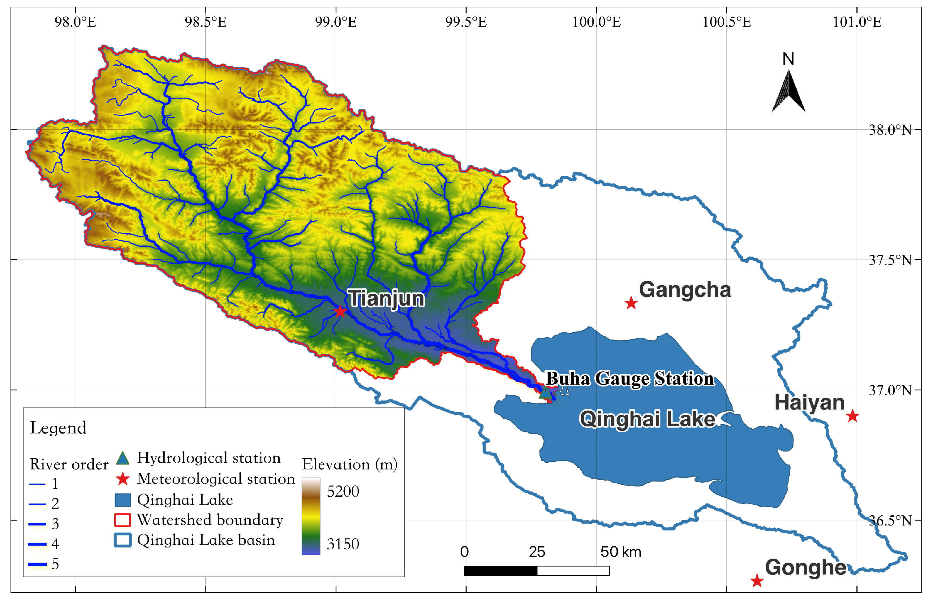
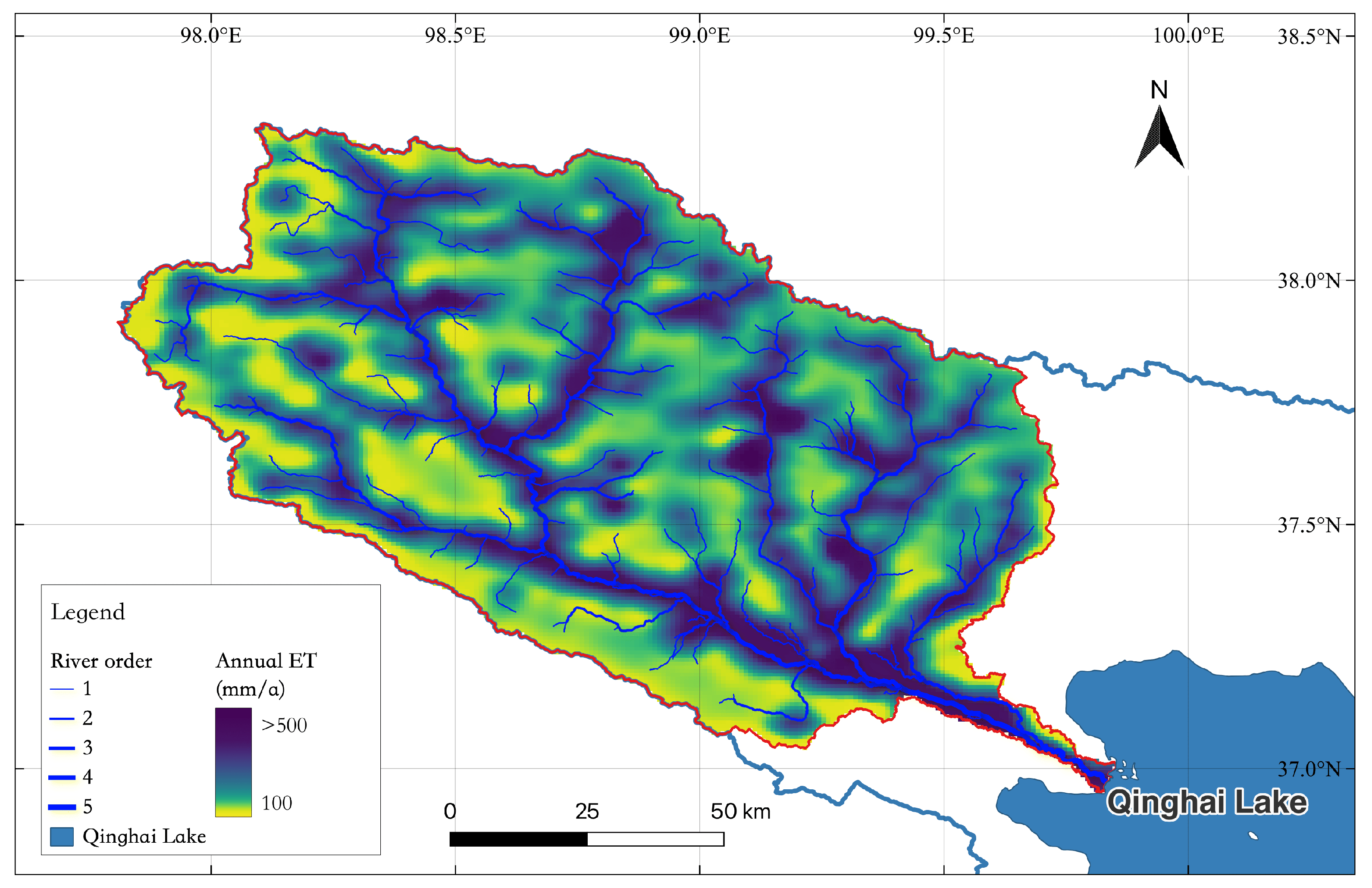
2.1. Study Area

The Qinghai Lake Basin is located in the northeastern part of the Tibetan Plateau, with coordinates between 97°50′ E and 101°20′ E, and 36°15′ N and 38°20′ N. It is a sensitive area to global climatic change and a region with vulnerable ecosystems. The basin exhibits strong catchment capabilities, predominantly featuring high-altitude areas ranging from 3194 to 5174 m, with terrain that decreases from the northwest to the southeast [18]. The Buha River, an important tributary in the basin, flows through Tianjun, Gangcha, and Gonghe Counties, originating from the Shule-Nanshan mountains in the northwest and flowing southeast to Qinghai Lake, covering approximately 286 km. The altitudes of the river source and mouth are about 4513 and 3195 m, respectively, and the watershed area is 1438 km².

The watershed’s climate is characterized by intense radiation, low temperatures, dryness, and low precipitation, with an average annual precipitation of about 430 mm, while potential evaporation exceeds 1600 mm. Precipitation mainly occurs from May to September and increases with altitude. No large reservoirs or other hydraulic infrastructures have been established in the watershed. The predominant vegetation types are alpine meadow, alpine steppe, and subalpine shrubs, which significantly influence the region’s hydrological processes. Detailed spatial information of the Qinghai Lake and Buha River watershed is shown in Figure 1.

2.2. Data

The construction of the SHUD model relies on three types of key data: land surface data, meteorological forcing data, and observational data. Land surface data are primarily used to establish hydrological parameters, meteorological data drive the model, and observational data are used for model calibration and validation.

The essential terrestrial data for modeling are retrieved from the Global Hydrological Data Cloud (GHDC, https://ghdc.ac.cn, accessed on 10 June 2023) Table 1. According to GHDC manuals, the Digital Elevation Model (DEM) originates from ASTER GDEM [24] and has a horizontal resolution of approximately 30 m (or 1 arc-second). Soil classification and texture data are obtained from the Harmonized World Soil Database (HWSD) v1.2 [25], with a resolution of 1 km. Land cover classification data are sourced from the MODIS land cover dataset presented by the United States Geological Survey (USGS) [26], with a resolution of 500 m.

The detailed explanation in Column 3 of Table 1 outlines the essential data needed to run the SHUD model. Although this study utilizes the specific datasets listed in Column 4, any data conforming to the requirements in Column 3 can be employed. For further details on what data are needed and their significance, please refer to [27], which provides an in-depth discussion on the detailed methodology for deploying the SHUD model in any given watershed.

Table 1. The data used for this study.

Data	Description	Variables	Source
Elevation	30 m	Elevation	ASTER GDEM [24]
Watershed Boundary	Vector polygon	Boundary	Generated from DEM delineation
River Network	Vector polylines	River reaches	Generated from DEM delineation
Landcover	500 m resolution	Land cover classes	USGS MODIS land cover data [26]
Soil	1 km resolution	Sand-silt-clay percentage, bulk density, organic matter	HWSD [25]
Meteorological Data	0.1 deg, 3 h interval	Precipitation, temperature, humidity, wind speed, radiation, pressure	CMFD [28]
Streamflow	-	Streamflow at gauge station of Buha River	Local hydrological department

Table 1. The data used for this study.

Data	Description	Variables	Source
Elevation	30 m	Elevation	ASTER GDEM [24]
Watershed Boundary	Vector polygon	Boundary	Generated from DEM delineation
River Network	Vector polylines	River reaches	Generated from DEM delineation
Landcover	500 m resolution	Land cover classes	USGS MODIS land cover data [26]
Soil	1 km resolution	Sand-silt-clay percentage, bulk density, organic matter	HWSD [25]
Meteorological Data	0.1 deg, 3 h interval	Precipitation, temperature, humidity, wind speed, radiation, pressure	CMFD [28]
Streamflow	-	Streamflow at gauge station of Buha River	Local hydrological department

Considering the scarcity of meteorological stations in the study area, the China Meteorological Forces Dataset (CMFD) [28] was chosen as the forcing data for the SHUD model in this study. The CMFD dataset covers all terrestrial areas of China for the period between 1979 and 2018. Despite the absence of data for the most recent years, the variable and spatial-temporal resolution meet the requirements of numerical hydrological models. The CMFD offers seven variables: near-surface air temperature, surface pressure, specific humidity, wind speed, downward shortwave and longwave radiation, and precipitation rate. It provides a temporal resolution of 3 h and a spatial resolution of 0.1 degrees. The simulation area contains 209 CMFD grids (see Figure 2). Observational streamflow data necessary for the study were provided by the Buha River Hydrological Station, located at 99°44′ E, 37°02′ N (see Figure 1). It covers daily streamflow between 1980 and 2017.

2.3. Model Construction

2.3.1. SHUD Model

The Simulator of Hydrologic Unstructured Domains (SHUD) is a distributed hydrological model that integrates high spatial-temporal resolution, multiple processes, multiple scales, and surface–subsurface interactions. The model performs calculations using unstructured triangular grids and the finite volume method, ensuring precise physical process descriptions and spatial-temporal continuity. Compared to semi-distributed models, such as SWAT, TOPMODEL, and VIC, the SHUD model provides a more comprehensive simulation of physical processes [29,30,31,32].

The SHUD model uses an adaptive time-step scheme, adjusting according to the convergence state of variables during running. The model supports simulations ranging from single hydrological events to long-term watershed water processes. It employs unstructured triangular grids, encompassing both regular and Delaunay irregular triangles, for detailed spatial partitioning of the watershed. This approach not only improves the simulation accuracy but also enables local dense or sparse partitioning of critical areas in the watershed, while effectively controlling the computation scale. The model employs a global implicit solver, which simultaneously solves hydrological processes, such as surface runoff and groundwater flow, guaranteeing the continuity, consistency, and convergence of the hydrological variables. The finite volume method and the internal algorithms jointly ensure the balance of global or local water quantity. The SHUD model effectively solves the problems associated with data handling and simulation efficiency caused by river curvature through the utilization of the cross-topology relationship between river channels and triangular elements.

Some of the critical hydrological processes are explained as follows:

• Snow accumulation and melt: Snow accumulation is computed using a temperature threshold-based rain–snow partitioning scheme, while snowmelt is calculated using a degree-day model.
• Evapotranspiration (ET): The model initially calculates potential evapotranspiration (PET) of forcing time-series data using the Penman–Monteith equation. Actual evapotranspiration for each triangular unit is then determined by multiplying PET by a soil moisture stress coefficient, which is derived from the soil moisture content in the unit.
• River and surface runoff routing: Both are computed using the Manning equation, though with notably different parameters for each.
• Infiltration, unsaturated and saturated flow: The calculation of these processes is governed by the Darcy–Richards equation, where hydraulic conductivity is the determinant parameter.

For more detailed information on these calculations, readers are directed to consult additional publications [27,31,32,33], which provide a comprehensive treatment of the model’s computational aspects.

The SHUD model has two main types of hydrological computational units (HCUs): triangular slope elements and linear river segments. The three-dimensional slope elements are designed as triangular prisms, divided vertically into the surface layer, unsaturated layer, and saturated layer, with an assumed impervious bedrock layer beneath. In the model, when the number of triangular elements is represented as $N_{\mathrm{ele}}$ and the number of river segments is $N_{\mathrm{riv}}$, the total number of HCUs amounts to $N=3\times N_{\mathrm{ele}}+N_{\mathrm{riv}}$. The SHUD model primarily computes the flux among HCUs. The calculation on the land surface includes snow accumulation/melt, infiltration, and surface lateral flow from/to neighboring units. The unsaturated zone processes vertical infiltration/exfiltration and moisture supply to the saturated area, including soil moisture, groundwater recharge, soil evaporation, and vegetation transpiration. The saturated zone handles lateral groundwater flow (or base flow) between triangular units and its exchange with the river network. Both unsaturated and saturated zones adjust potential evapotranspiration in response to soil water content and groundwater level.

The SHUD model has already been applied in various areas, including water resource issues, the impact of land cover change, the impact of climate change, lake dynamics, and runoff forecasting [7,31,32,34].

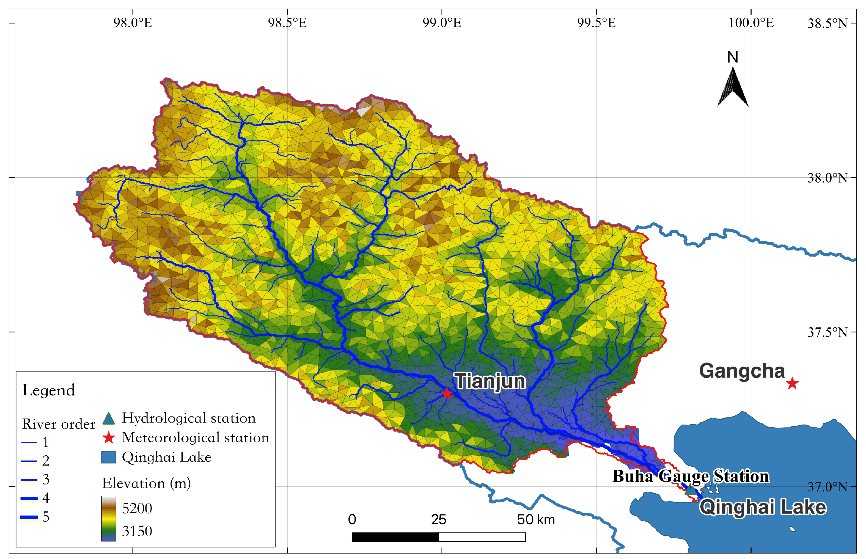
2.3.2. Model Configuration

The construction of the SHUD model includes data access and model deployment. We retrieved the necessary terrestrial and forcing data from the Global Hydrological Data Cloud (GHDC, https://ghdc.ac.cn) and deployed the model using the rSHUD package and AutoSHUD automation script within the R environment [27]. The data downloaded from GHDC are listed in Table 1, and the detailed steps of model deployment can be found in [27]. The source code for deployment is shared on Zenodo [35].

The computational domain of the Buha River watershed consists of 1372 triangular elements and 660 river units, covering a total area of 14,487.1 km². Each triangular element has an average area of approximately 10.5 km², with an equivalent spatial resolution of about 3.2 km (as shown in Figure 2). The total length of the river network is 4122 km, averaging approximately 2.5 km per river segment. This watershed has a single outlet, which flows directly into Qinghai Lake.

2.3.3. Model Parameter Calibration

The initial conditions for the model were established based on the results of 40 years of simulation from 1979 to 2018. Specifically, the state of variables, such as snowpack, vegetation interception, surface water, soil water, and groundwater at the end of the simulation on 31 December 2018, was used as the initial conditions. Following this, the model proceeded to an automatic parameter calibration.

The automated model parameter calibration employed the Covariance Matrix Adaptation Evolution Strategy (CMA-ES) [27,31,36]. This technique maximizes the agreement between model predictions and observational data by effectively exploring the parameter space while simultaneously avoiding convergence to local optima in nonlinear hydrological model parameter calibration. The number of samples in each generation is $\lambda$, the maximum number of generations is $N_{\max }$, and the threshold of “best” objective function is $G^0$. The indices of samples and generations are i and j, respectively; therefore, i ranges [0, $\lambda$] and j ranges [0, $N_{\max }$]. ${\theta }_j^i$ indicates the parameter set in the j generation and the ith sample. In our calibration $N_{\max }=20$, $\lambda =120$. The calibration process was carried out on a computing cluster, based on the following workflow:

• Initialization of the CMA-ES algorithm.
• Random sampling parameter sets (${\Theta }_j=C[{\theta }_j^1,{\theta }_j^2,\dots ,{\theta }_j^{\lambda })$]) within a predefined parameter range.
• Conduct $\lambda$ parallel simulation tasks using these parameter sets.
• Upon completion of parallel simulations, compare simulation results with observational data and compute the best objective function value $G^{*}$ in this generation. Computation ceases if the best objective function value $G^{*}$ exceeds a preset threshold $G^0$ ($G^{*}>G^0$) or if the maximum number of iterations $N_i$ has been reached ($N_i>N_{\max }$). Continue otherwise.
• Select the most optimal parameter set based on the objective function value to seed the next generation of parameter sampling (${\Theta }_{j+1}^i$). Introduce additional perturbation based on the covariance of parameters and result, repeat random sampling within parameter space to generate new $\lambda$ parameter sets.
• Repeat steps (3) to (5).

The Nash–Sutcliffe Efficiency (NSE) was adopted as the objective function for model calibration. The NSE value ranges from negative infinity to 1, where an NSE value of 1 indicates a perfect match between model simulations and observations. According to the literature, a daily streamflow simulation is considered acceptable if the NSE value is greater than 0.36, while it is deemed to be good if the NSE value is above 0.5 [37,38,39]. For monthly streamflow simulations, where precision requirements are higher, an acceptable NSE threshold is above 0.5 and a good NSE threshold is above 0.7. The best NSE value of daily streamflow in the CMA-ES algorithm was set as 0.2. In addition to the NSE, model performance evaluation also includes the Kling–Gupta Efficiency (KGE) and the coefficient of determination R². Here, KGE is a single indicator that combines correlation, bias, and variability, where KGE = 1 indicates a perfect match. The range for R² is [0,1], where R² = 1 also indicates perfect agreement.

Informed by studies indicating that 2004 was a critical turning point from a decline to an increase in the water level of Qinghai Lake [5,7], this research adopts 2003 as the cut-off point for model calibration and validation. The calibration-validation process included 3 years of model spin-up period (1990–1992), 10 years of parameter calibration period (1993–2002), and 9 years of parameter validation period (2003–2011). For the validation, the model must repeat the simulation from 1990 to 2011 with the optimal parameter set which covers the spin-up, calibration, and validation periods. The model evaluation is based on the simulated results over a continuous 22-year period (1990–2011).

3. Results

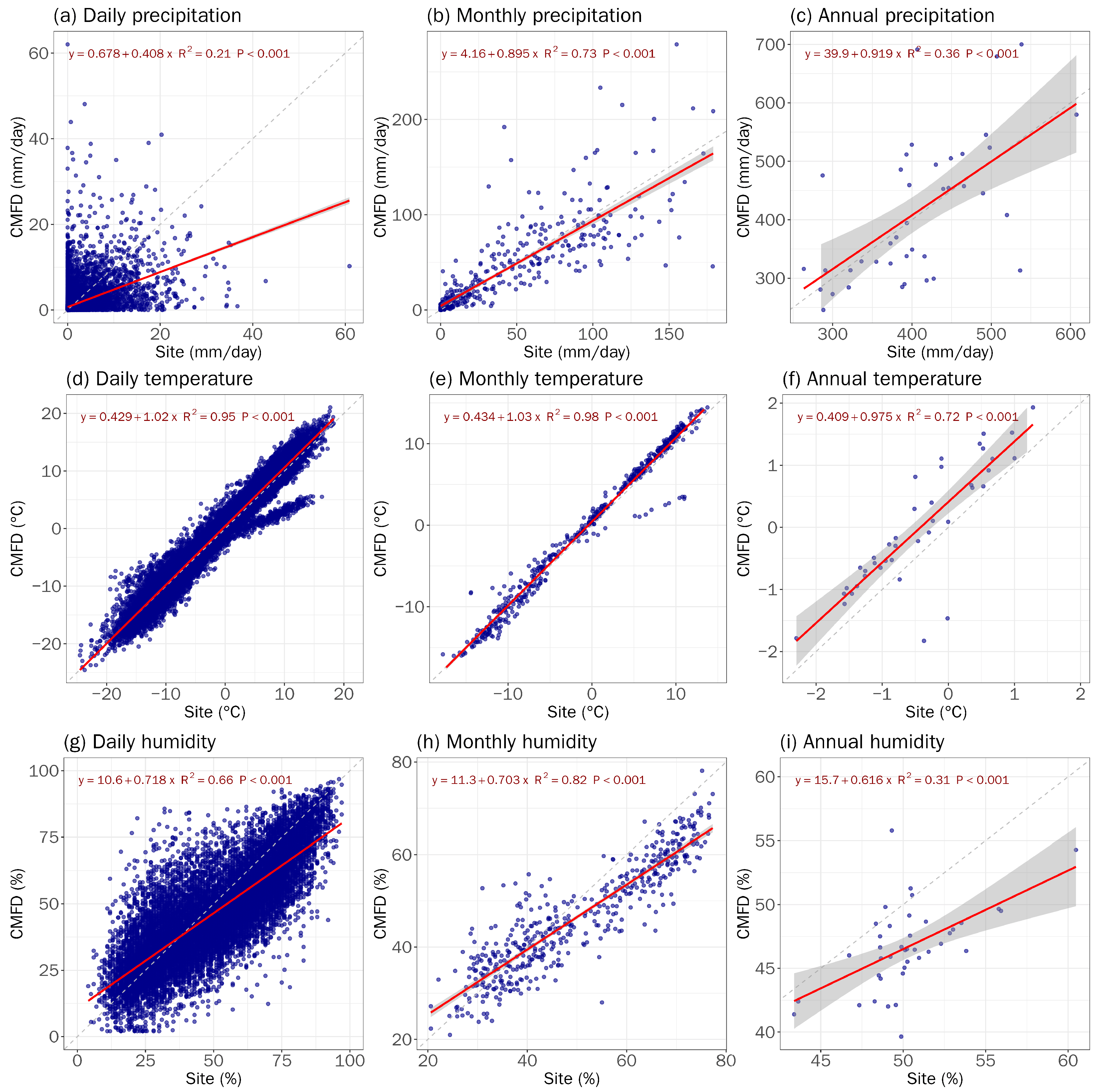
3.1. Evaluation of CMFD Data

We assessed the usability of meteorological data and the basic characteristics of watershed streamflow, integrating the data from meteorological stations, reanalysis data, and hydrological station streamflow information. CMFD grid data located at 99.05° E and 37.25° N were compared with the meteorological data from Tianjun station (Figure 1 and Figure 2). The meteorological reanalysis data offered by CMFD are every 3 h, while the Tianjun meteorological station provides daily data.

After comparative analysis, significant differences were found in the daily, monthly, and yearly scales of precipitation, temperature, and relative humidity within the CMFD data (see Figure 3). On a daily scale, discrepancies in precipitation data were especially evident. CMFD data underestimate precipitation intensity and cannot accurately represent daily extreme rainfall events. This uncertainty introduced at the daily scale seriously undermines the precision of the streamflow simulation. On a monthly scale, there is good consistency between CMFD precipitation data and observed site data with a linear fitting slope of 0.895 (R² = 0.73), indicating a satisfactory performance of CMFD data at the monthly scale. However, there are considerable differences between CMFD and local observation due to the minimal amount of data at the annual scale.

Overall, the temperature data from CMFD align well with the observed site data. On daily, monthly, and yearly scales, the intercept of the fitted line is approximately 0.4 °C, and the slope is close to 1, suggesting that CMFD data are slightly higher than the observed data. On daily and monthly scales, the temperature data within the 5–10 °C range exhibit abnormal outliers differing from other data; the specific reason remains to be further analyzed. For the relative humidity, the CMFD data perform reasonably well at the daily and monthly scales and are acceptable, but overall it tends to be dry.

Precipitation and energy input are crucial determinants in dictating the hydrological balance of a watershed. Precipitation offers the material foundation to a watershed, influencing the formation of surface runoff and groundwater, while parameters such as temperature, humidity, wind speed, and radiation directly constrain the evaporation process within a watershed. The water balance equation for a watershed can be expressed as: $\Delta S=P-E-Q$, where $\Delta S$ represents the change in the water storage of the watershed, P is the precipitation, E is the total evapotranspiration, and Q denotes streamflow. In a long-term analysis, the change in watershed water storage tends to zero, implying that $P=E+Q$. Consequently, the summation of the ET ratio ($E/P$) and the runoff ratio ($Q/P$) in a watershed should be equal to 1.

The historical mean annual precipitation and temperature fluctuation trends in the Buha River watershed, based on CMFD data, show that the annual average precipitation is approximately 435 mm (Figure 4). Despite considerable inter-annual fluctuations, an overall gradual increasing trend is observed, with a growth rate of about 2.63 mm/year (R² = 0.13, p < 0.05). Over 40 years, the mean annual temperature is around −4 °C, albeit with significant rising trends, at a warming rate of roughly 0.05 °C/year (R² = 0.54, p < 0.005). Although, over the past 40 years, the increase in the precipitation level of the Buha River watershed is modest, the temperature consistently rises. This progressive increase in precipitation and temperature potentially impacts the local water cycle processes.

Notably, however, despite the lack of apparent turning points identified via statistical analysis, there are some deviations among the inter-annual fluctuation curves of the two variables. The evaluation of precipitation, temperature, and runoff ratio over the past 40 years through the Mann–Kendall trend detection method indicates that precipitation and temperature data, based on CMFD, do not exhibit noticeable abrupt changes. However, a change in the runoff ratio is discernible. Two runoff ratios are calculated: one is the observed streamflow in the Buha River over CMFD precipitation data (QR1), and the other is the observed streamflow over precipitation data from the Tianjun meteorological station (QR2). The annual runoff ratio varies from 0.05 to 0.36. The outcome of the Mann–Kendall abrupt change detection method reveals that QR1 and QR2 experienced a significant rise in 2007, indicating the presence of a break in the growth of the runoff ratio around this year (p < 0.05). Setting 2007 as a boundary, the average runoff ratio from 1980 to 2007 is around 0.12. But between 2001 and 2018, it rises to about 0.21, indicating a significant surge in the runoff ratio (Figure 5). This finding coincides with several studies asserting that the rapid growth in the Qinghai Lake level in recent years is due to the considerable increase in streamflow [5,7].

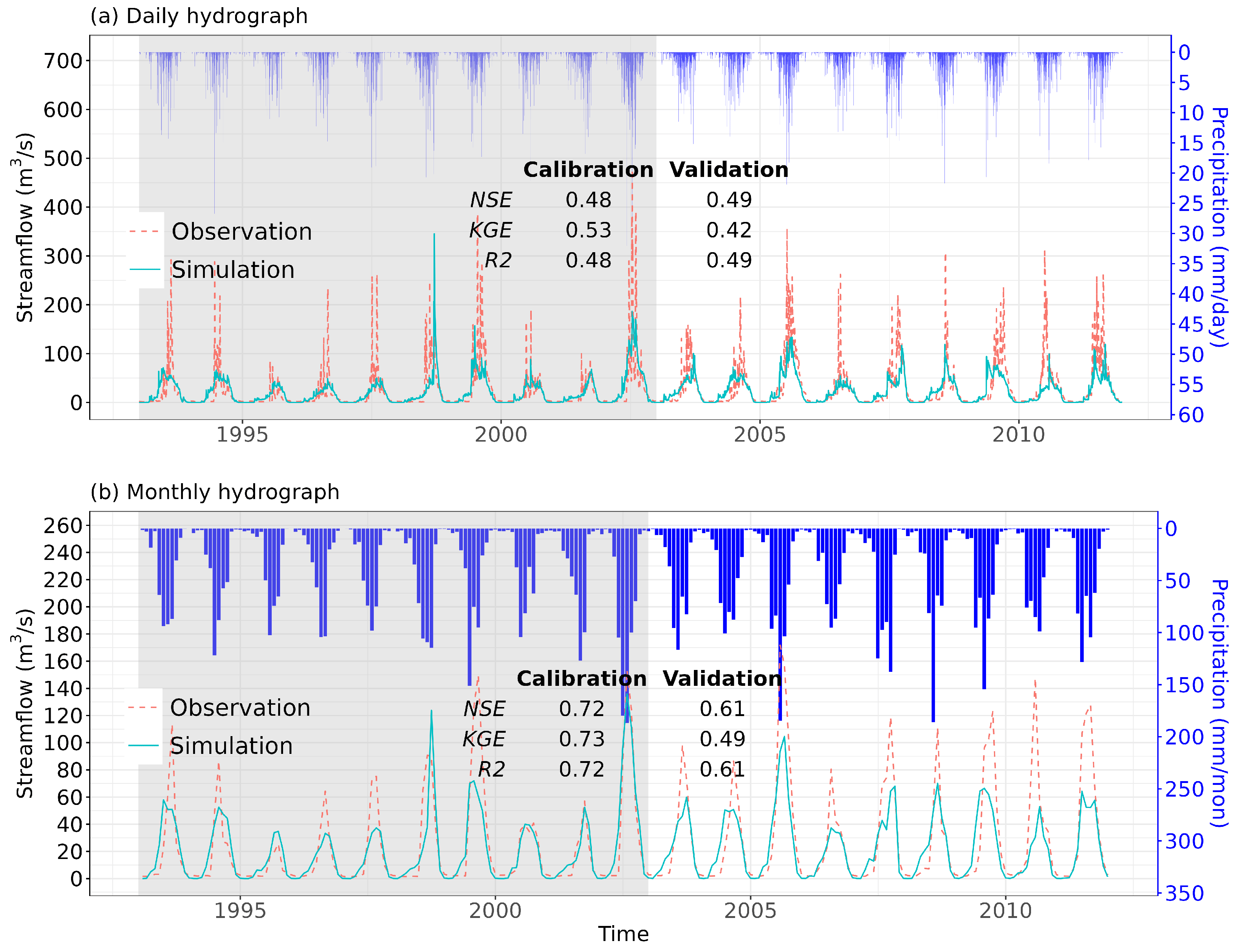
3.2. Evaluation of SHUD Model

In terms of daily streamflow simulation, the SHUD model, after parameter optimization using the CMA-ES methodology, realized NSE values of 0.48 and 0.49 for the calibration and validation phases, respectively. Similarly, the KGE values were 0.53 and 0.42, with R² values of 0.48 and 0.49, respectively (Figure 6a). The indicators suggest that, albeit that the model has some predictive capabilities, the overall accuracy is yet to reach an ideal level. It is notable that the NSE is slightly lower during the calibration phase compared to the validation phase. This could be attributable to the model’s strong dependence on the input meteorological data, which influences the accuracy of the simulation.

About the monthly streamflow simulation, the SHUD model exhibited more remarkable results than the daily scale. The NSE values for the calibration and validation phase were 0.72 and 0.61, respectively, with corresponding KGE values of 0.73 and 0.49, and R² values of 0.72 and 0.61 (Figure 6b). These indicators are within a very good range [37,38,39], indicating that the model can effectively capture the change patterns in monthly hydrological dynamics. However, the precision of daily scale simulation is limited by the quality of the CMFD daily precipitation data that we analyzed in the previous section, namely, the uncertainty in daily precipitation data has a direct impact on the accuracy of daily streamflow simulation.

Considering multiple model evaluation standards [39,40,41], adjusting the parameter set has enabled the daily streamflow simulation capacity to reach a good usability level, while the monthly streamflow simulation performance shows excellent usability. Considering the purpose of this study, which targets analyzing long-term hydrological characteristics, the high simulation accuracy based on monthly streamflow suffices. The SHUD model’s strong correlation with the observed monthly streamflow data from the Buha River watershed shows that the model is suitable for hydrological forecasting and water resource management over the watershed.

3.3. River Hydrological Balance

The annual variance in the river’s water storage is essentially zero, so the water balance equation for the river reads: $Q_s+Q_g=Q$. In this equation, $Q_s$ denotes the volume of surface runoff injected into the river (56.7 $\times {10}^9{\mathrm{m}}^3{\mathrm{a}}^{-1}$), $Q_g$ represents the groundwater supply to the river (29 $\times {10}^9{\mathrm{m}}^3{\mathrm{a}}^{-1}$), and Q is the total streamflow at an outlet of the river network (27.8 $\times {10}^9{\mathrm{m}}^3{\mathrm{a}}^{-1}$). This indicates that the river’s water sources primarily originate from surface runoff while replenishing surrounding groundwater.

In the cold and alpine regions, the interaction between the river and groundwater is frequent. When the groundwater level of the hillslope is higher than the river stage, groundwater replenishes the river; in contrast, if the river stage exceeds the groundwater level, leakage from the river to groundwater occurs. The output of the SHUD model reveals the interaction between the river network and surrounding groundwater in the watershed (refer to Figure 7). Figure 7b depicts the spatial distribution of river recharge and leakage as well as the spatial distribution of groundwater levels. The spatial distribution of groundwater is deduced from the difference between the SHUD model’s output of groundwater storage and aquifer thickness, and then converted into raster data through inverse distance weighting (IDW) spatial interpolation. The groundwater level is closely related to topography, where regions far from the river with steep slopes have lower groundwater tables, while areas near the river with large drainage areas and gentle slopes have higher tables.

The replenishment–leakage relationship in the river network of the Buha River watershed dynamically varies from upstream to downstream, sometimes replenishing groundwater and at times leaking. However, the long-term trend shows that the river primarily leaks to surrounding groundwater. The annual total volume of groundwater leakage is 1.46 $\times {10}^9{\mathrm{m}}^3$ and the total volume of groundwater replenishing the river is 0.73 $\times {10}^9{\mathrm{m}}^3$; therefore the net leakage volume of the river is 0.73 $\times {10}^9{\mathrm{m}}^3$ per year. The groundwater replenishment rate per unit length of the river is 1.25 ${\mathrm{m}}^3{\mathrm{km}}^{-1}{\mathrm{a}}^{-1}$, and the leakage rate is 0.76 ${\mathrm{m}}^3{\mathrm{km}}^{-1}{\mathrm{a}}^{-1}$.

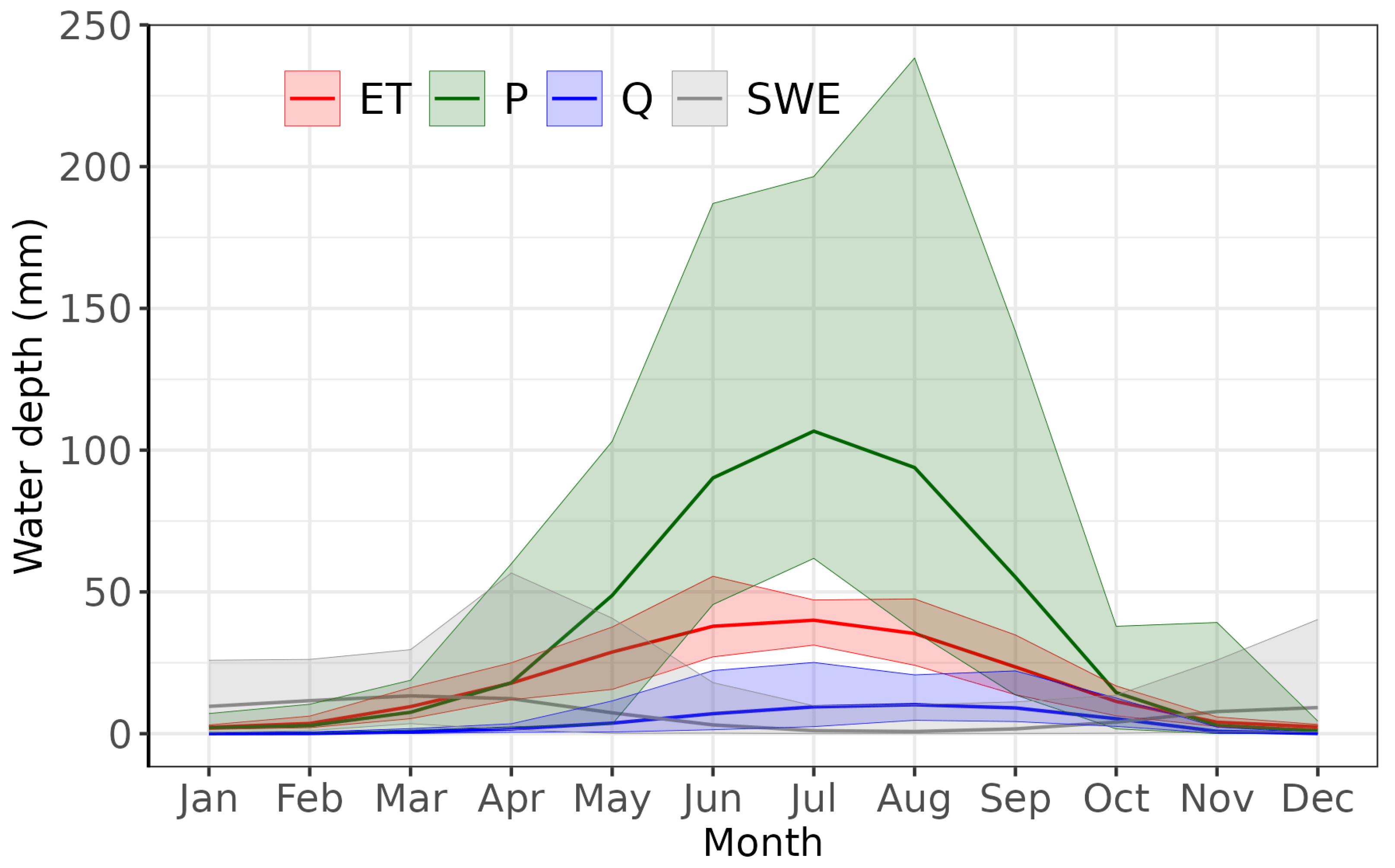
3.4. Water Balance

The long-term water balance equation for the Buha River watershed is articulated as $P=E+Q$, where P is the total precipitation, E is the actual ET, and Q is the streamflow in the statistical period. The E and Q are results from the SHUD simulation. Seasonal variations in the water balance are substantial within this region, as illustrated in Figure 8. This is mainly attributed to the unique climatic characteristic of the Buha River watershed, namely, the concurrency of high temperatures and monsoons causes the precipitation, evaporation, and streamflow to peak during the summertime. Figure 8 provides a detailed depiction of multi-year monthly averages of precipitation, streamflow, actual ET, and snowfall, alongside their maximum and minimum values. Precipitation predominantly occurs from May to October (92% of annual precipitation), with a higher proportion of snowfall in November and May of the following year, while streamflow is mainly concentrated from May to September (89% of annual streamflow). Annually, rainfall displays considerable fluctuations, as well as snowfall, indicating significant unpredictability in the region’s precipitation pattern.

Regarding precipitation and snowfall, they exhibit significant annual variability, possibly linked to regional climatic changes and seasonal weather patterns. In contrast, the annual fluctuations in streamflow and actual ET are rather minimal. Snowfall plays a crucial role in water balance, with snow present within the region from October to the subsequent May, and its annual fluctuation is significant, substantially impacting the available surface water and spring streamflow.

The variability in actual ET is influenced by multiple factors, primarily the availability of energy and soil water. In the Buha River watershed, areas closer to the river experience higher soil humidity due to elevated groundwater levels, consequently resulting in relatively high actual ET (see Figure 9). The spatial disparity in actual ET is mainly determined by soil water content, while the physical properties of the soil and vegetation cover significantly affect the ET process. Additionally, topographic features, such as slope and orientation, influence the surface’s energy absorption and the evaporative capability of water, indirectly impacting the spatial distribution of actual ET.

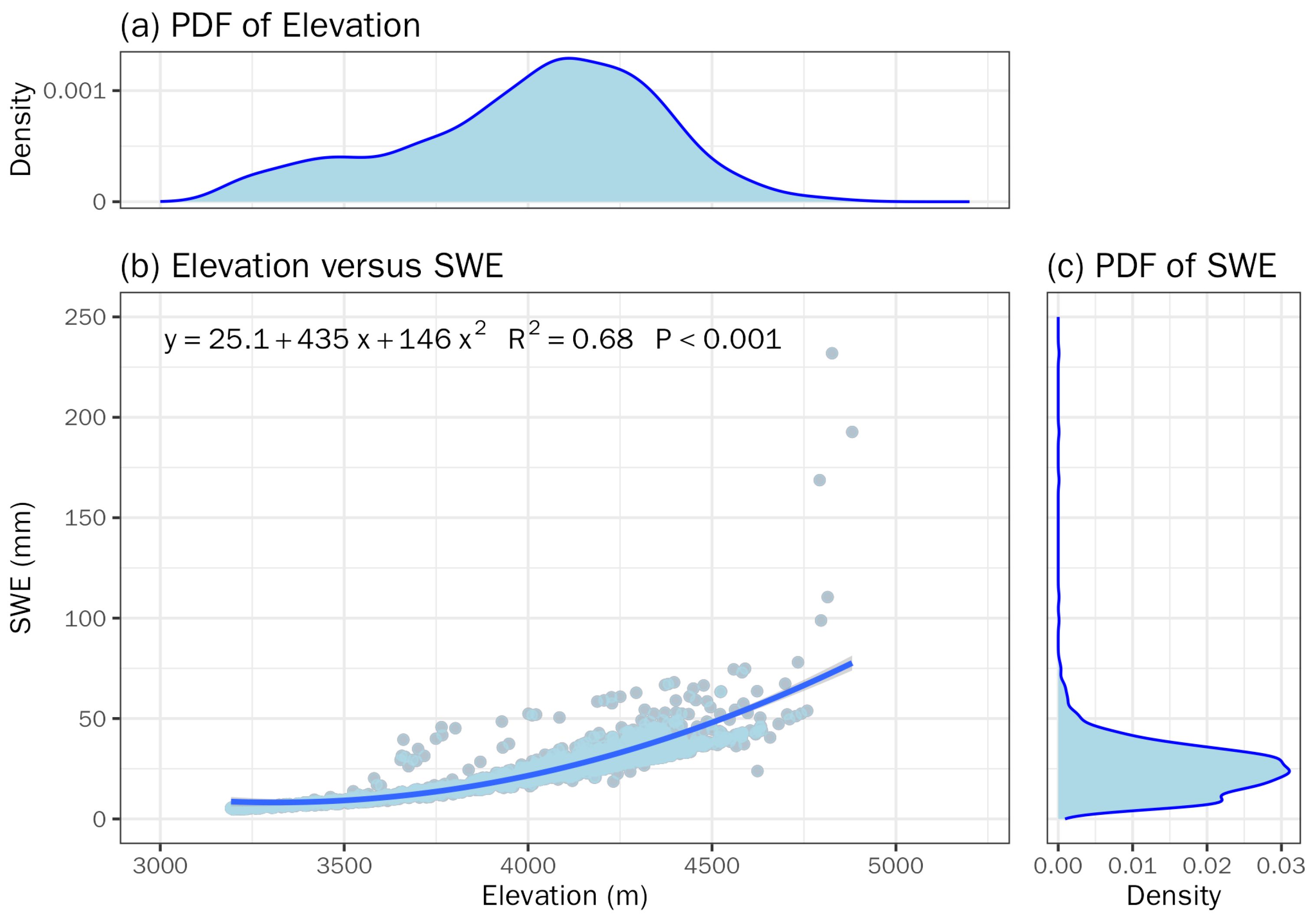
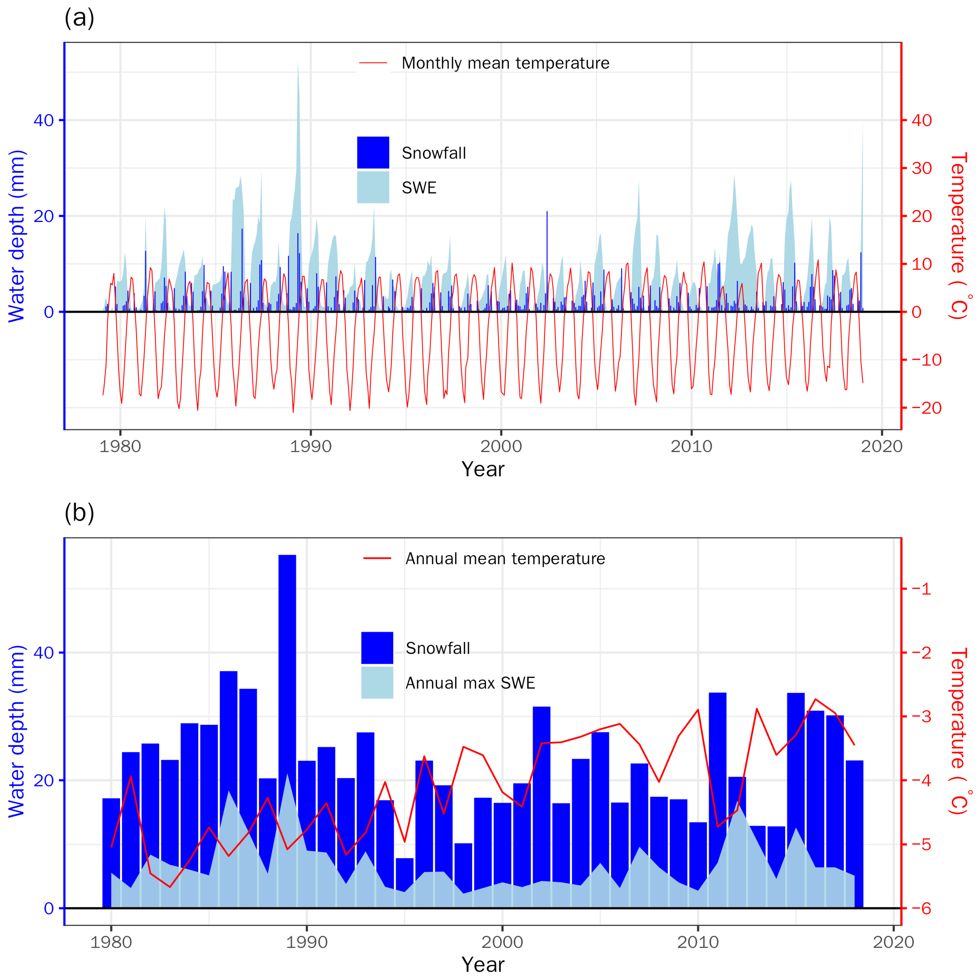
3.5. Snowfall

The snow water equivalent (SWE) distribution within the Buha River watershed exhibits a strong correlation with altitude, as shown in Figure 10 and Figure 11. The raster map is also the result of IDW spatial interpolation from SWE values on SHUD triangles. The computational units of the SHUD model span an altitudinal range from 3192 m to 4881 m, with the yearly maximum snow depth varying between 4 mm and 232 mm (refer to Figure 10a,c). The volume of snowfall escalates with increasing altitude, revealing a nonlinear growth relationship (refer to Figure 10b).

Figure 11 delineates the spatial distribution of the annual maximum snow water equivalent in the watershed. The snowfall peaks in the mountainous regions of the northwest; as the altitude diminishes, the annual maximum snow water equivalent gradually reduces. In the high-altitude peripheries of the watershed, the yearly average snow water equivalent exceeds 40 mm, while in the regions adjacent to the downstream river and Qinghai Lake, the annual average snowfall usually remains less than 20 mm.

The distribution of snowfall is affected not only by altitude but also exhibits significant seasonal and interannual variations. Based on the snow–rain separation and snow–melt schemes of the SHUD model, Figure 12 depicts the monthly cumulative snowfall and melting, juxtaposed against the temperature and precipitation changes over the past 40 years. Typically, the snow within the watershed fully melts in summer; however, in certain years, for example, 2011–2012, the snowfall did not entirely melt but accumulated into the following year. The hydrological year (September of the prior year to August of the current year) reveals that the accumulation and melting of snowfall occur simultaneously on a monthly and yearly scale, with the annual snowfall consistently exceeding the annual maximum cumulative snow (Figure 12). The watershed-wide average annual snowfall fluctuates between 7.8 mm and 55.3 mm, with a mean of approximately 23.2 mm; the variation in snow water equivalent ranges from 2.3 mm to 21.0 mm, with a multi-annual average of 6.9 mm.

4. Discussion

The present study employs CMFD data to drive the SHUD model in efforts to analyze the hydrological characteristics of the Buha River watershed. The analysis results significantly depend on the accuracy of the CMFD data as well as the reliability of the SHUD model’s structure and parameters. Consequently, the following three aspects of uncertainty exist in this study:

(1)

Data-driven uncertainty: While the CMFD data offer high temporal and spatial resolution and cover the entire study area, thereby representing a valuable data source for numerical hydrological simulation, a comparison of the grid data with corresponding site data reveals a reasonable agreement at monthly and annual scales. However, a substantial deviation is encountered at the daily scale, especially for the precipitation data. This introduces uncertainty when the SHUD model is driven with sub-daily scale data, leading to less reliable daily streamflow and other variables on a daily scale. Therefore, our analysis primarily relies on monthly and yearly hydrological data.

(2)

Model structure uncertainty on frozen soil: There are permafrost and frozen soil within this area which affect the hydrological processes in the watershed [42]. The frozen soil parameterization in the SHUD model is indeed based on the nonlinear response of hydraulic properties to accumulated temperature, drawing from simplified permafrost frost index algorithms as noted in [42,43,44]. Specifically, the key parameter of hydraulic conductivity decreases with falling accumulated temperatures (below zero), significantly impacting both lateral and vertical water flows across each triangular unit within the model domain. These effects cumulatively influence the hydrographic characteristics and the streamflow of the watershed at the basin scale. However, as rightly pointed out, this approach does not fully capture the coupled heat–water physical processes. Addressing this issue is a crucial direction for the future development of the SHUD model. So, prospective integration of advanced models that feature coupled water and heat dynamics is needed to provide a more comprehensive treatment of water–heat–vegetation interactions.

(3)

Parameter uncertainty: Despite employing the Covariance Matrix Adaptation Evolution Strategy (CMA-ES) for automatic calibration, which is efficient and can find the global optimum, multiple parameter sets show acceptable performance, exhibiting the “equifinality” phenomenon [45,46,47,48]. This indicates that parameter uncertainty still exists. Future simulations and analyses for this watershed should consider employing multi-parameter ensemble simulations for a more comprehensive investigation of the resulting uncertainty.

Though the Buha River watershed is the largest in Qinghai Lake, research targeting this region and available data remain insufficient. More data are needed in the future to validate and enhance this study. Owing to present uncertainties in data and models, it is imperative to continue research in the future.

5. Conclusions

This paper utilizes data from the CMFD and implements the SHUD numerical hydrology model to simulate the variation in streamflow and other hydrological characteristics in the Buha River watershed from 1979 to 2018. The outcomes are examined against meteorological station data and model simulation results, facilitating an analysis of the meteorological and streamflow characteristics in the Buha River over the past 40 years. The following conclusions are drawn:

• The monthly datasets from CMFD align accurately with observed data, although there is a lack of precision in reflecting daily precipitation intensity characteristics. A slight deviation has been observed in temperature and relative humidity over various time scales. Over the past four decades, an ascending trend in precipitation and temperature in the Buha River watershed has been observed, despite the absence of a significant abrupt change.
• The SHUD model exhibits promising accuracy on a monthly scale when fitting observed streamflow data, demonstrating its applicability to hydrological forecasts and water resource management within the Buha River watershed.
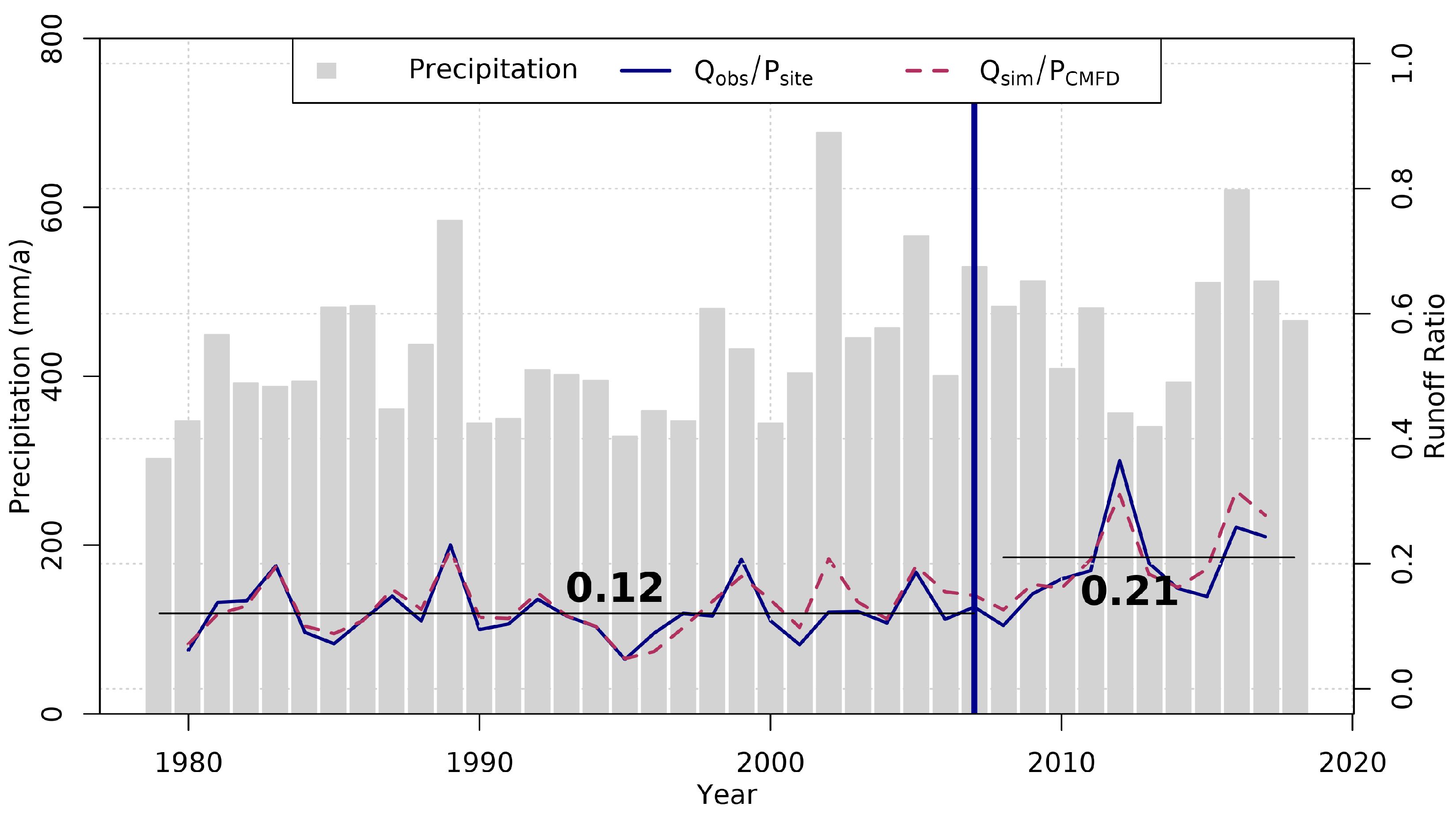
• Runoff ratios for the Buha River are low, fluctuating annually between 0.11 and 0.21. Notably, fluctuations in the runoff ratios around 2007 are closely related to the turning point in the Qinghai Lake stage from a downward to an upward trend.
• Within the analysis of water balance in river channels, leakage and replenishment along the river show spatial alteration, with a net leakage over long-term periods. However, no perceptible spatial difference has been observed between leakage and replenishment.
• In the Buha River watershed, snow accumulation increases with altitude, and in most years, the accumulated snow completely melts within the same year. On a seasonal scale, the increase in streamflow coincides with the onset of snowmelt, making a significant contribution to streamflow replenishment at the end of cold seasons.

Although the Buha River basin is the largest and most crucial basin of Qinghai Lake, research literature on the Buha River remains sparse due to a lack of data and limited human activity. The analysis and findings of this study provide a deeper understanding of the hydrological dynamics in the Buha River watershed. Moreover, they also highlight key areas for future study, particularly focusing on the continual improvement in dataset accuracy and model parameter optimization.

References

- Zhang, H. Analysis of Changes in Hydrological Elements of Lakes on the Qinghai-Tibet Plateau Based on Remote Sensing and Their Response to Climate Change. Ph.D. Thesis, Liaocheng University, Liaocheng, China, 2018. [Google Scholar]
- Li, X.; Zhang, T.; Yang, D.; Wang, G.; He, Z.; Li, L. Research on lake water level and its response to watershed climate change in Qinghai Lake from 1961 to 2019. Front. Environ. Sci. 2023, 11, 1130443. [Google Scholar] [CrossRef]
- Li, L.; Shen, H.; Liu, C.; Xiao, R. Response of water level fluctuation to climate warming and wetting scenarios and its mechanism on Qinghai Lake. Clim. Chang. Res. 2020, 16, 600–608. [Google Scholar]
- Lanzhou Branch of Chinese Academy of Sciences. Environmental Evolution and Prediction in Qinghai Lake; Science Press: Beijing, China, 1994. (In Chinese) [Google Scholar]
- Cui, B.; Li, X. Runoff processes in the Qinghai Lake Basin, Northeast Qinghai-Tibet Plateau, China: Insights from stable isotope and hydrochemistry. Quat. Int. 2015, 380–381, 123–132. [Google Scholar] [CrossRef]
- Cui, B.; Li, X. The impact of climate changes on water level of Qinghai Lake in China over the past 50 years. Hydrol. Res. 2016, 47, 532–542. [Google Scholar] [CrossRef]
- Shu, L.; Li, X.; Chang, Y.; Meng, X.; Chen, H.; Qi, Y.; Wang, H.; Li, Z.; Lyu, S. Advancing understanding of lake–watershed hydrology: A fully coupled numerical model illustrated by Qinghai Lake. Hydrol. Earth Syst. Sci. 2024, 28, 1477–1491. [Google Scholar] [CrossRef]
- Qin, Q.; Huang, Q. Simulation of energy and water budget of Qinghai Lake, China. Chin. J. Oceanol. Limnol. 1998, 16, 289–297. [Google Scholar]
- Li, X.; Xu, H.; Sun, Y.; Zhang, D.; Yang, Z. Lake-level change and water balance analysis at lake Qinghai, West China during recent decades. Water Resour. Manag. 2007, 21, 1505–1516. [Google Scholar] [CrossRef]
- Li, X.; Xiao, J.; Li, F.; Xiao, R.; Xu, W.; Wang, L. Remote Sensing Monitoring of the Qinghai Lake Based on EOS/MODIS Data in Recent 10 Years. J. Nat. Resour. 2012, 27, 1962–1970. [Google Scholar]
- Li, X.; Zhao, H.; Wang, G.; Yao, K.; Xin, Q.; He, Z.; Li, L. Influence of watershed hydrothermal conditions and vegetation status on lake level of Qinghai Lake. Arid Land Geogr. 2019, 42, 499–508. [Google Scholar]
- Shi, X.; Li, L.; Wang, Q.; Liu, B.; Zhang, H.; Liu, Z. Climatic Change and Its Influence on Water Level of Qinghai Lake. Meteorol. Sci. Technol. 2005, 33, 58–62. [Google Scholar]
- Fang, J.; Li, G.; Rubinato, M.; Ma, G.; Zhou, J.; Jia, G.; Yu, X.; Wang, H. Analysis of Long-Term Water Level Variations in Qinghai Lake in China. Water 2019, 11, 2136. [Google Scholar] [CrossRef]
- Dong, H.; Song, Y.; Zhang, M. Hydrological trend of qinghai lake over the last 60 years: Driven by climate variations or human activities? J. Water Clim. Chang. 2019, 10, 524–534. [Google Scholar] [CrossRef]
- Zhang, C.; He, L.; Wang, L. Climate Evolution Characteristics of Water Resources in Buha River Basin. South North Water Transf. Water Sci. Technol. 2017, 15, 45–49+57. [Google Scholar]
- Li, Y.; Li, X.; Cui, B.; Peng, H.; Yi, W. Trend of streamflow in Lake Qinghai basin during the past 51 years (1956–2007)—Take Buha River and Shaliu River for examples. J. Lake Sci. 2010, 22, 757–766. [Google Scholar]
- Zhang, N. Study on the Variation of Runoff in Buha River. Qinghai Sci. Technol. 2002, 36–38. (In Chinese) [Google Scholar]
- Huang, X.; Li, R.; Gan, Y.; Wu, Y. Attribution analysis of runoff change in Buha River basin based on Budyko hypothesis. South North Water Transf. Water Sci. Technol. 2023, 21, 480–490, (In Both Chinese and English). [Google Scholar]
- Zhou, Y.; Chen, H.; Zhang, S.; Huang, Y. Simulating the influence of climate change on hydrological proceses at Buha River basin of Qinghai Lake by SWIM. J. Beijing Norm. Univ. 2017, 53, 208–214. [Google Scholar] [CrossRef]
- Wang, H.; Li, D.; Lei, Y.; Zhang, M. Application of Topmodel in Runoff Simulation in Buha River Basin. Water Conserv. Sci. Technol. Econ. 2016, 22, 8–12. [Google Scholar]
- Long, Y.; Zhang, Y.; Zhao, G.; Yan, P.; Li, Q.; Li, R. The Uncertainty in Meteorological and Hydrological Proceses Modeled by Using SWAT Model—A Case Study in the Buhachu River Basin. J. Glaciol. Geocryol. 2012, 34, 660–667. [Google Scholar]
- Zhang, G.; Xie, H.; Yao, T.; Li, H.; Duan, S. Quantitative water resources assessment of Qinghai Lake basin using Snowmelt Runoff Model (SRM). J. Hydrol. 2014, 519, 976–987. [Google Scholar] [CrossRef]
- Su, D.; Wen, L.; Gao, X.; Leppäranta, M.; Song, X.; Shi, Q.; Kirillin, G. Effects of the Largest Lake of the Tibetan Plateau on the Regional Climate. J. Geophys. Res. Atmos. 2020, 125, e2020JD033396. [Google Scholar] [CrossRef]
- NASA; METI; AIST; Japan Spacesystems; U.S./Japan ASTER Science Team. ASTER Global Digital Elevation Model V003. 2018. Available online: https://lpdaac.usgs.gov/products/astgtmv003/ (accessed on 1 July 2024).
- Nachtergaele, F.; van Velthuizen, H.; Verelst, L.; Batjes, N.; Dijkshoorn, J.; van Engelen, V.; Fischer, G.; Jones, A.; Montanarella, L.; Petri, M.; et al. Harmonized World Soil Database (Version 1.2); Food and Agric Organization of the UN (FAO): Rome, Italy; International Institute for Applied Systems Analysis (IIASA): Laxenburg, Austria; ISRIC—World Soil Information: Wageningen, The Netherlands; Inst of Soil Science-Chinese Acad of Sciences (ISS-CAS): Nanjing, China; EC-Joint Research Centre (JRC): Brussels, Belgium, 2008. [Google Scholar]
- Broxton, P.D.; Zeng, X.; Sulla-Menashe, D.; Troch, P.A. A Global Land Cover Climatology Using MODIS Data. J. Appl. Meteorol. Climatol. 2014, 53, 1593–1605. [Google Scholar] [CrossRef]
- Shu, L.; Ullrich, P.; Meng, X.; Duffy, C.; Chen, H.; Li, Z. rSHUD v2.0: Advancing the Simulator for Hydrologic Unstructured Domains and unstructured hydrological modeling in the R environment. Geosci. Model Dev. 2024, 17, 497–527. [Google Scholar] [CrossRef]
- He, J.; Yang, K.; Tang, W.; Lu, H.; Qin, J.; Chen, Y.; Li, X. The first high-resolution meteorological forcing dataset for land process studies over China. Sci. Data 2020, 7, 25. [Google Scholar] [CrossRef] [PubMed]
- Freeze, R.; Harlan, R. Blueprint for a physically-based, digitally-simulated hydrologic response model. J. Hydrol. 1969, 9, 237–258. [Google Scholar] [CrossRef]
- Hrachowitz, M.; Clark, M.P. HESS Opinions: The complementary merits of competing modelling philosophies in hydrology. Hydrol. Earth Syst. Sci. 2017, 21, 3953–3973. [Google Scholar] [CrossRef]
- Shu, L.; Chang, Y.; Wang, J.; Chen, H.; Li, Z.; Zhao, L.; Meng, X. A brief review of numerical distributed hydrological model SHUD. Adv. Earth Sci. 2022, 37, 680–691. [Google Scholar]
- Shu, L.; Chen, H.; Meng, X.; Chang, Y.; Hu, L.; Wang, W.; Shu, L.; Yu, X.; Duffy, C.; Yao, Y.; et al. A review of integrated surface-subsurface numerical hydrological models. Sci. China Earth Sci. 2024, 67, 1459–1479. [Google Scholar] [CrossRef]
- Shu, L.; Ullrich, P.A.; Duffy, C.J. Simulator for Hydrologic Unstructured Domains (SHUD v1.0): Numerical modeling of watershed hydrology with the finite volume method. Geosci. Model Dev. 2020, 13, 2743–2762. [Google Scholar] [CrossRef]
- Shu, L. Impacts of Urbanization and Climate Change on the Hydrological Cycle: A Study in Modern and Ancient Land Use Change. Ph.D. Thesis, The Pennsylvnia State University, University Park, PA, USA, 2017. [Google Scholar]
- Shu, L.; Chang, Y. Model and data for “Comprehensive Hydrological Analysis of the Buha River Watershed with High-Resolution SHUD Modeling”. In Comprehensive Hydrological Analysis of the Buha River Watershed with High-Resolution SHUD Modeling (v0.1); Zenodo: Geneva, Switzerland, 2024. [Google Scholar] [CrossRef]
- Hansen, N. The CMA Evolution Strategy: A Comparing Review. In Towards a New Evolutionary Computation; Springer: Berlin/Heidelberg, Germany, 2016; pp. 75–102. [Google Scholar] [CrossRef]
- Gupta, H.V.; Kling, H.; Yilmaz, K.K.; Martinez, G.F. Decomposition of the mean squared error and NSE performance criteria: Implications for improving hydrological modelling. J. Hydrol. 2009, 377, 80–91. [Google Scholar] [CrossRef]
- Li, X.; Long, D.; Slater, L.J.; Moulds, S.; Shahid, M.; Han, P.; Zhao, F. Soil Moisture to Runoff (SM2R): A Data-Driven Model for Runoff Estimation Across Poorly Gauged Asian Water Towers Based on Soil Moisture Dynamics. Water Resour. Res. 2023, 59, 1169–1188. [Google Scholar] [CrossRef]
- Santhi, C.; Arnold, J.G.; Williams, J.R.; Dugas, W.A.; Srinivasan, R.; Hauck, L.M. Validation of the SWAT Model on a Large River Basin with Point and Nonpoint Sources. JAWRA J. Am. Water Resour. Assoc. 2001, 37, 1169–1188. [Google Scholar] [CrossRef]
- Moriasi, D.N.; Arnold, J.G.; Van Liew, M.W.; Bingner, R.L.; Harmel, R.D.; Veith, T.L. Model Evaluation Guidelines for Systematic Quantification of Accuracy in Watershed Simulations. Trans. ASABE 2007, 50, 885–900. [Google Scholar] [CrossRef]
- Moriasi, D.N.; Gitau, M.W.; Pai, N.; Daggupati, P. Hydrologic and water quality models: Performance measures and evaluation criteria. Trans. ASABE 2015, 58, 1763–1785. [Google Scholar] [CrossRef]
- Gao, H.; Wang, J.; Yang, Y.; Pan, X.; Ding, Y.; Duan, Z. Permafrost Hydrology of the Qinghai-Tibet Plateau: A Review of Processes and Modeling. Front. Earth Sci. 2021, 8, 576838. [Google Scholar] [CrossRef]
- Nelson, F.E.; Outcalt, S.I. A Computational Method for Prediction and Regionalization of Permafrost. Arct. Alp. Res. 1987, 19, 279–288. [Google Scholar] [CrossRef]
- Walvoord, M.A.; Kurylyk, B.L. Hydrologic Impacts of Thawing Permafrost—A Review. Vadose Zone J. 2016, 15, 1–20. [Google Scholar] [CrossRef]
- Ebel, B.A.; Loague, K. Physics-based hydrologic-response simulation: Seeing through the fog of equifinality. Hydrol. Process. 2006, 20, 2887–2900. [Google Scholar] [CrossRef]
- Beven, K. Towards an alternative blueprint for a physically based digitally simulated hydrologic response modelling system. Hydrol. Process. 2002, 16, 189–206. [Google Scholar] [CrossRef]
- Beven, K. A manifesto for the equifinality thesis. J. Hydrol. 2006, 320, 18–36. [Google Scholar] [CrossRef]
- Savenije, H.H. Equifinality, a blessing in disguise? Hydrol. Process. 2001, 15, 2835–2838. [Google Scholar] [CrossRef]
Disclaimer/Publisher’s Note: The statements, opinions and data contained in all publications are solely those of the individual author(s) and contributor(s) and not of MDPI and/or the editor(s). MDPI and/or the editor(s) disclaim responsibility for any injury to people or property resulting from any ideas, methods, instructions or products referred to in the content. |
© 2024 by the authors. Licensee MDPI, Basel, Switzerland. This article is an open access article distributed under the terms and conditions of the Creative Commons Attribution (CC BY) license (https://creativecommons.org/licenses/by/4.0/).
Share and Cite
Chang, Y.; Li, X.; Shu, L.; Ji, H. Comprehensive Hydrological Analysis of the Buha River Watershed with High-Resolution SHUD Modeling. Water 2024, 16, 2015. https://doi.org/10.3390/w16142015
Chang Y, Li X, Shu L, Ji H. Comprehensive Hydrological Analysis of the Buha River Watershed with High-Resolution SHUD Modeling. Water. 2024; 16(14):2015. https://doi.org/10.3390/w16142015
Chicago/Turabian StyleChang, Yan, Xiaodong Li, Lele Shu, and Haijuan Ji. 2024. "Comprehensive Hydrological Analysis of the Buha River Watershed with High-Resolution SHUD Modeling" Water 16, no. 14: 2015. https://doi.org/10.3390/w16142015