Article

SWAT-Driven Exploration of Runoff Dynamics in Hyper-Arid Region, Saudi Arabia: Implications for Hydrological Understanding

by
Sajjad Hussain
1,*,
Burhan Niyazi
1,
Amro Mohamed Elfeki
1,2,
Milad Masoud
3,4,
Xiuquan Wang
5,6 and
Muhammad Awais
5,6
1
Department of Water Resources, Faculty of Environmental Sciences, King Abdulaziz University, Jeddah 21589, Saudi Arabia
2
Irrigation and Hydraulics Department, Faculty of Engineering, Mansoura University, Mansoura 35516, Egypt
3
Water Research Center, King Abdulaziz University, Jeddah 21598, Saudi Arabia
4
Hydrology Department, Desert Research Centre, Cairo 11753, Egypt
5
Canadian Centre for Climate Change and Adaptation, University of Prince Edward Island, Charlottetown, PE C1A 4P3, Canada
6
School of Climate Change and Adaptation, University of Prince Edward Island, Charlottetown, PE C1A 4P3, Canada
*
Author to whom correspondence should be addressed.
Water 2024, 16(14), 2043; https://doi.org/10.3390/w16142043
Submission received: 16 June 2024 / Revised: 10 July 2024 / Accepted: 17 July 2024 / Published: 19 July 2024

Abstract

:
Hydrological modeling plays a vital role in water-resource management and climate-change studies in hyper-arid regions. In the present investigation, surface runoff was estimated by a Soil and Water Assessment Tool (SWAT) model for Wadi Al-Aqul, Saudi Arabia. The Sequential Uncertainty Fitting version 2 (SUFI-2) technique in SWAT-CUP was adopted for the sensitivity analysis, calibration, and validation of the SWAT model’s components. The observational runoff data were scarce and only available from 1979 to 1984; such data scarcity is a common problem in hyper-arid regions. The results show good agreement with the observed daily runoff, as indicated by a Pearson Correlation Coefficient (r) of 0.86, a regression (R2) of 0.76, and a Nash–Sutcliffe coefficient (NSE) of 0.61. Error metrics, including the Mean Absolute Error (MAE) and Root Mean Square Error (RMSE), were notably low at 0.05 and 0.58, respectively. In the daily validation, the model continued to perform well, with a correlation of 0.76 and regression of 0.58. As a new approach, fitted parameters of daily calibration were incorporated into the monthly simulation, and they demonstrated an even better performance. The correlation coefficient (regression) and Nash–Sutcliffe were found to be extremely high during the calibration period of the monthly simulation, reaching 0.97 (0.95) and 0.73, respectively; meanwhile, they reached 0.99 (0.98) and 0.63 in the validation period, respectively. The sensitivity analysis using the SUFI-2 algorithm highlighted that, in the streamflow estimation, the Curve Number (CN) was found to be the most responsive parameter, followed by Soil Bulk Density (SOL_BD). Notably, the monthly results showed a higher performance than the daily results, indicating the inherent capability of the model in regard to data aggregation and reducing the impact of random fluctuations. These findings highlight the applicability of the SWAT model in predicting runoff and its implication for climate-change studies in hyper-arid regions.

1. Introduction

Water-resource management comprises several interconnected components with significant economic, environmental, ecological, and social consequences [1,2,3]. The computation of hydrological parameters is essential in the hydrological cycle, required for water resource optimization, flood control, and water-resource management [4,5,6]. According to the Intergovernmental Panel on Climate Change (IPCC)’s findings, the observed warming over the last few decades has led to notable changes in the hydrological cycle, including higher evapotranspiration rates, shifts in precipitation patterns, and, consequently, variations in runoff dynamics [7,8]. Several studies have indicated that extreme climatic events have significantly increased over the past few decades [9,10]. These changes underscore the need to accurately estimate hydrological parameters for effective water-resource management and planning. However, the interactions among key variables, such as rainfall, land use/land cover (LULC), and soil properties, are complex and challenging to measure directly. Hydrological models are therefore frequently employed in both scientific research and practical applications to estimate these parameters and their interactions with each other [11,12]. These models provide critical insights and predictions that inform strategies for managing water resources in a changing climate.
There are different types of models that have been used to simulate the hydrological cycle [13,14,15]. Distributed models are regarded to have the potential to improve the predictions of hydrologic processes since they can include a variety of land features and spatial precipitation datasets [16,17]. The Soil and Water Assessment Tool (SWAT) is a widely used, semi-distributed, and complex hydrological model with multi-purpose objectives, including the estimation of surface runoff, evapotranspiration, groundwater recharge, and sediment load calculation [18,19,20]. In strongly arid regions with limited data availability, the SWAT model remains a valuable tool because of its capability to incorporate soil, meteorological, vegetation, and basin characteristics [21]. A research conducted by Pandi et al. [22] found the SWAT model to be a reliable tool for land and water-resource management. Their study estimated the water-balance components in a catchment of Tamil Nadu, India, for 20 years (2001–2020). The results revealed that the coefficient of determination (R2) for the model output was 0.75 in pre-calibration and 0.94 in post-calibration. Similarly, Diriba [23] conducted research with surface-runoff modeling using meteorological data for the last 30 years (1987–2016) in the SWAT model. The model calibrated for 9 years (1994–2003) and validated for 8 years (2004–2011) of streamflow data. The results highlighted that, during calibration, the R2 (NS) was found to be 0.82 (0.70), while in the validation, it touched R2 = 0.78, indicating a good modeling approach by the SWAT model. In another study, Marahatta et al. [24] employed the SWAT model to define the rainfall-runoff behavior of a complex mountainous basin in Central Nepal. Their results indicated that the model over- and underestimated the flow for some years, but its overall performance was very good after calibration. Several other studies have suggested that the SWAT model is beneficial for assessing runoff and other hydrological parameters, facilitating planning for sustainable land management [25,26,27,28].
Previous studies have demonstrated the good performance of the SWAT model in perennial river catchments. However, there is a lack of research assessing its performance in hyper-arid regions like Al-Madinah Al-Munawarah, Saudi Arabia. To address this gap, the main objective of this study was to evaluate the accuracy of the SWAT model in predicting daily and monthly runoff in a hyper-arid region. This research is novel in regard to several aspects, as it represents the pioneering and comprehensive application of the SWAT model within this hyper-arid environment. Furthermore, the sensitivity analysis identified the most influential parameters for runoff generation, providing valuable guidelines for similar regions. Additionally, the study demonstrates the direct applicability of daily calibrated parameters to monthly simulations in large and hyper-arid basins, significantly streamlining the modeling process. The existing study provides a significant contribution by demonstrating the applicability and reliability of the SWAT model in such challenging environments. Future studies can be conducted by integrating a calibrated SWAT model with climate models to accurately project the hydrological conditions in such hyper-arid regions.

2. Material and Method
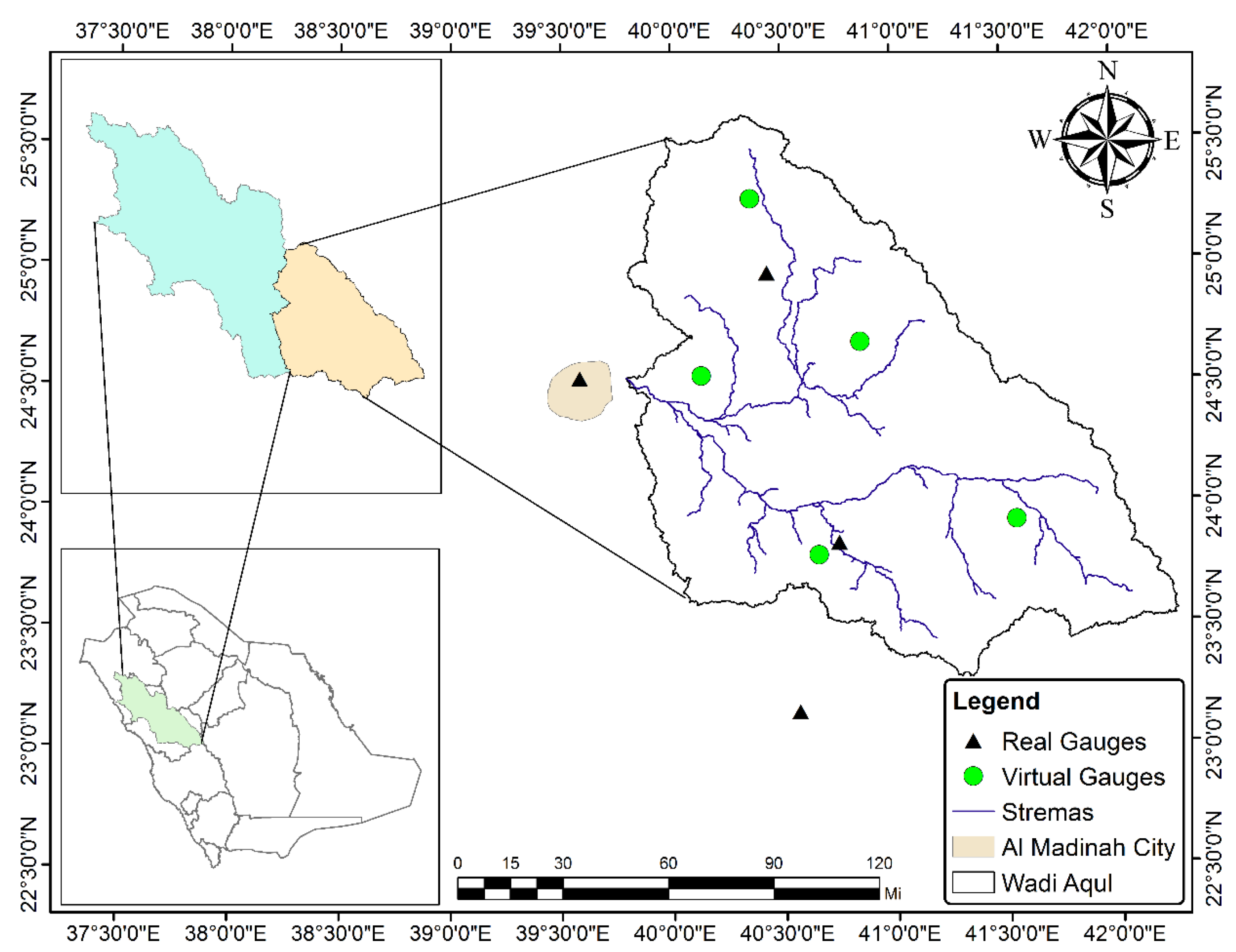
2.1. Study Area

The study area (Wadi Al-Aqul) is located in Al-Madinah Al-Munawarah Province of Saudi Arabia, stretches between 25°38′ to 23°30′ N and 39°40′ to 42°06′ E, toward the east side of Al-Madina City. Geographically, Al-Madina Al-Munawarah Province is surrounded by Makkah Al-Mukarramah Province on the south, Riyadh Province on the southeast, the Red Sea on the west, Tabuk province on the north, and Hail Province on the northeast, as shown in Figure 1. Al-Madinah Al-Munawarah City is the most important part of this region due to its religious importance and remain crowded throughout the year for pilgrims visit to Prophet Muhammad’s (peace be upon him) and his mosque, making it important region for hydrological studies. Hydrologically, different Wadies surround Al-Madinah City, and all of these Wadies are the sub-basins of a very large basin named Wadi Al-Hamad (as indicated in the lower left subsection, in light blue color of Figure 1). Among these sub-basins is the currently selected Wadi Al-Aqul, which is one of the largest, and it is importantly situated in the east of the city, covering an area of 35,584 km2. The climate has been characterized as hyper-arid due to the low annual rainfall (~50 mm), as per criteria defined by [29]. Most of the rainfall predominantly occurred from November to February. The province experiences varying temperatures, with hot and dry summers and mild winters, exhibiting peak mean air temperatures of 36.5 °C in August and minimum mean temperatures of 17.7 °C in January [30].

2.2. Metrological and Streamflow Dataset

The climatic dataset that contains rainfall and minimum and maximum temperature was collected from the Ministry of Environment, Water, and Agriculture (MEWA). The rainfall data were available at four real gauges (actual measurement stations) that reside within and nearby the study area. These real gauges provide direct measurements of rainfall at specific locations. However, the existing watershed is very large and exhibits significant spatial variability in rainfall, necessitating a more detailed approach to accurately represent rainfall distribution across the entire area.
To address this, virtual gauges were constructed in each sub-basin. Virtual gauges are not physical devices but are instead points where rainfall estimates are interpolated based on data from the real gauges. These virtual gauges help to provide a finer resolution of rainfall distribution within the sub-basins, ensuring that spatial variability is effectively captured. There are various methods for rainfall interpolation, but the inverse distance weighting (IDW) technique is recognized as one of the most effective, as highlighted by References [31,32]. This method assigns more weight to rainfall measurements from closer real gauges when estimating rainfall at a virtual gauge. After performing the IDW interpolation, the virtual gauges were established to provide accurate rainfall estimates for each sub-basin. The temperature dataset was collected from Al-Madinah Al-Munawarah Airport for the same study period. The runoff data were available only for 6 years (1979–1984) years; therefore, respective climatic variables were also collected for same time span. Rainfall intensity, along with their respective hydrograph, can be seen in Figure 2.

2.3. Digital Elevation Model

The SWAT model requires topographic attributes (area, slope, slope length, channel length, channel slope, channel width, and channel depth) of the catchment, which are derived from a Digital Elevation Model (DEM) with spatial resolutions ranging from 10 to 90 m. For this study, the DEM from the global Shuttle Radar Terrain Mission (SRTM) was downloaded from the USGS website (https://earthexplorer.usgs.gov (accessed on 1 March 2023)) and has a spatial resolution of 30 m, as shown in Figure 3. The acquired DEM was pre-processed prior to its use in the SWAT model for hydrological delineation. This pre-processing included the sub-setting, filling, and re-projection of the DEM. The elevation in the Wadi ranges from 634 to 1821 m above mean sea level (AMSL), indicating higher peaks in the northern and southwestern edges, with a relatively flat area in the middle.

2.4. Land Use Land Cover Map
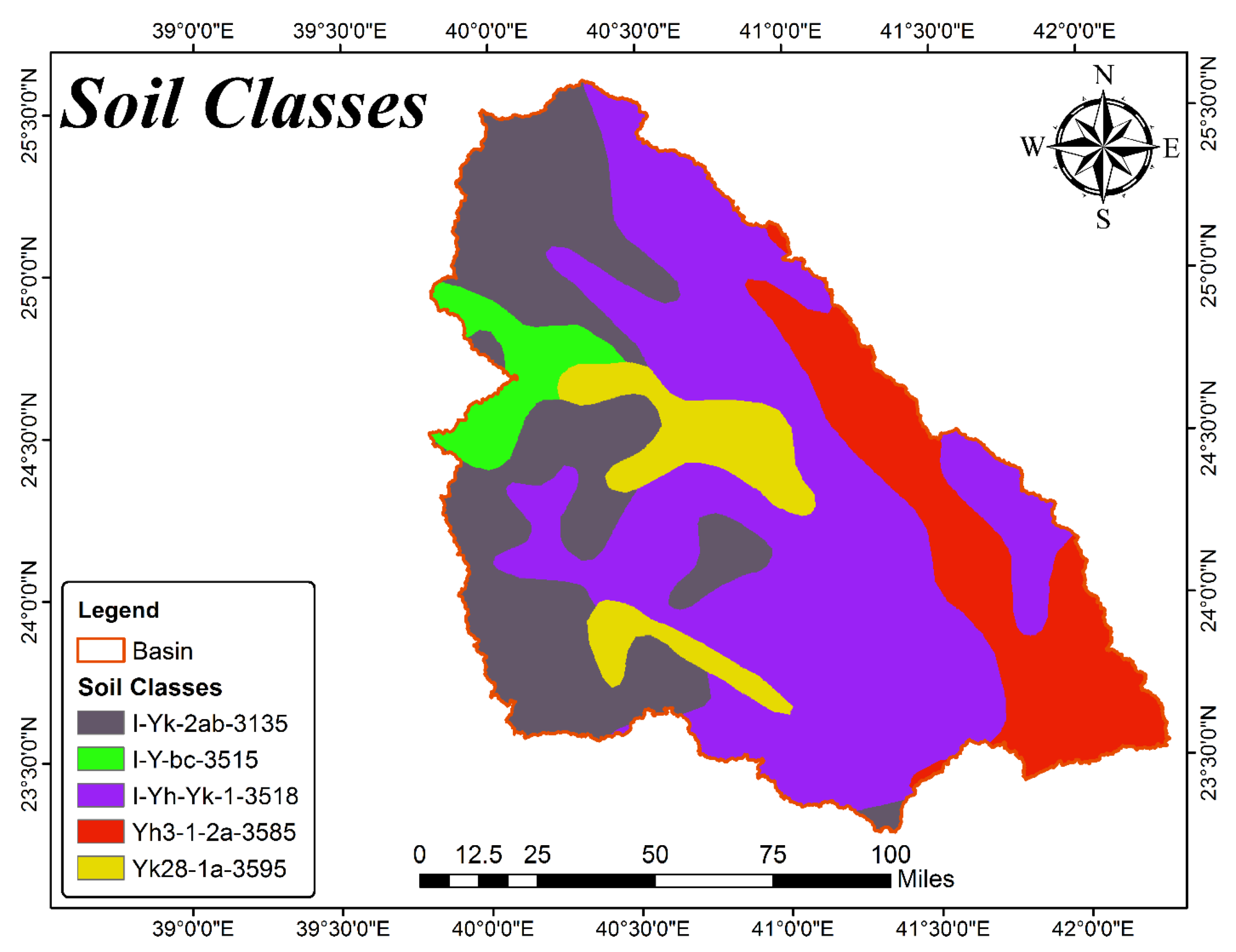
The LULC map is an important parameter that affects different hydrological components in the watershed. In this study, the LULC map was generated by Landsat 8 satellite imagery (30 × 30 m), using Google Earth Engine and GIS as the processing platforms. A supervised machine-learning algorithm, i.e., decision tree, was used in this methodology to classify the acquired images of Landsat. Based on land-use types, the area of the whole watershed was sub-divided into four categories, as shown in Table 1.
The spectral signatures of each land-cover class were obtained using spectral indices, specifically the Normalized Difference Vegetation Index (NDVI), Normalized Difference Built-Up Index (NDBI), and Normalized Difference Water Index (NDWI), along with visual interpretation for the best results. These indices were used to enhance the identification and differentiation of various land-cover types. For example, NDVI was used to identify vegetation cover by using the difference between red and near-infrared reflectance. NDBI was employed to distinguish between built-up and other areas, while NDWI was utilized to detect water bodies in the study region. Detailed descriptions and uses of these indices can be seen in References [33,34]. By analyzing the values of these spectral indices, we were able to create distinct spectral signatures for each class, facilitating accurate classification and mapping. Most of the area in the watershed consists of bare soil (sand + rocks), as shown in Figure 4. However, a very minor (<1%) area has vegetation and built-up areas, with no surface water body due to the hyper-arid climate.

2.5. Soil Map

The soil map utilized in this study was acquired from the Food and Agriculture Organization (FAO) database (https://data.apps.fao.org/map/catalog (accessed on 1 March 2023)). This soil database has been used in numerous research studies [35,36,37] for SWAT applications. The map was partitioned into numerous polygons, as depicted in Figure 5. Each polygon comprises a variety of unique properties associated with the soils that are present in the study area. The properties considered in this study included the hydrological soil group, hydraulic conductivity, soil texture, and other physical and chemical characteristics that were standardized using the FAO soil database. In order to synchronize the soil data with the watershed, the polygons were subjected to a clipping process. Soil characteristics for calibration were estimated by the Soil–Plant–Air–Water (SPAW) model [38], based upon the soil type and infiltration analysis [30] of the study area. Within the study area, five distinct soil classes were identified, each contributing differently to the watershed. Loam soil was the dominant soil in the region, covering 77% of the total area, and the other 23% was covered by sandy loam, as shown in Table 2.

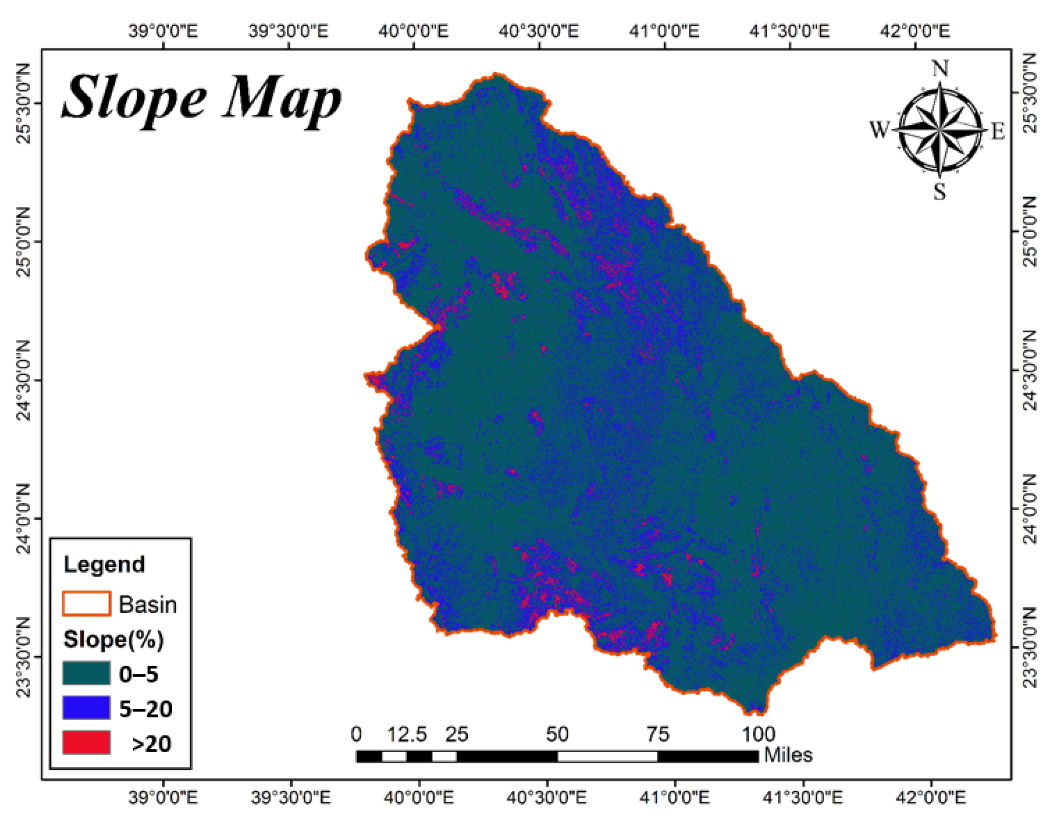
2.6. Watershed Slope

The importance of establishing multiple slope classifications becomes evident when dealing with sub-basins that exhibit a diverse range of topography. To better understand the implications of slope on hydrological processes, we utilized Digital Elevation Models (DEMs) to delineate the watershed’s boundaries and extract valuable sub-basin parameters. Slope is systematically categorized into three distinct classes to correspond with the characteristics of the Wadi Al-Aqul watershed: 0% to 5%, 5% to 20%, and exceeding 20%. These classifications are integral to our hydrological modeling approach. By adopting these slope categories, we enhance the precision of our modeling efforts. The visual representation of these slope classifications allows us to effectively capture the complex variations in slope characteristics, as depicted in Figure 6.

2.7. Hydrological Response Units (HRU’s)

In SWAT, a basin is typically partitioned into numerous watersheds (sub-basins) to account for spatial heterogeneity related to land use and land cover (LULC), soil composition, and topography. These sub-basins are further subdivided into regions characterized by uniform land-use patterns, soil characteristics, and slope gradients. These delineated areas are referred to as Hydrologic Response Units (HRUs). The SWAT model works on water-balance estimation with an assumption that individual HRUs have similar hydrological characteristics and behaviors [39]. HRUs serve to enhance the precision of forecasted outcomes within the sub-basin. However, although having numerous HRUs in a small sub-basin is not recommended, it is suggested to have a number of HRUs in large sub-basins [23]. Therefore, in the current study, we performed a reclassification in order to establish the Hydrological Response Units (HRUs), which serve as crucial elements in SWAT hydrological modeling. In the SWAT model, the HRU threshold determines the minimum area for aggregating land use, soil, and slope classes within each HRU. In delineating Hydrological Response Units (HRUs) for our study, we employed specific threshold values to define meaningful spatial units that capture variations in soil type, slope gradient, and land use/land cover (LULC). For soil, we utilized a threshold of 5% slope gradient to differentiate between areas with distinct hydrological behaviors. Similarly, for slope, we employed a threshold of 5% to delineate terrain units that influence runoff generation and flow pathways significantly. This helped in segregating different slope classes based on their potential for surface runoff. Regarding LULC, we used a 0% threshold due to the minor extent of land-cover classes in the study area, as used in [40]. This approach facilitated the creation of HRUs that capture the sparse vegetation and minimal land-use variations without compromising the model’s ability to simulate runoff dynamics effectively. For the current study, based on the similarities in watersheds, reclassification resulted in 121 HRUs, with most being in Sub-Basin 2.

2.8. Methodology

In this research, the Soil and Water Assessment Tool (SWAT) model was utilized to examine surface runoff for a large watershed, named Wadi Al-Aqul. Initially, the accomplishment of this essential work was facilitated through the utilization of the SWAT-2012 interface that was seamlessly incorporated into the Geographic Information System (GIS). The delineation was performed using the SWAT delineator, using the pre-processing (Re-projection, filling and sub-setting) of DEM. Detailed procedural guidance for this step can be found in the publications by [41]. Following the successful delineation of the catchment, the subsequent phase involved establishing and characterizing Hydrologic Response Units (HRUs), which relied on three critical spatial datasets: slope, land use/land cover, and soil maps. Slope classes were generated by the DEM, while the LULC map was generated by Landsat 8 imagery, using the supervised machine-learning algorithm, as discussed in the LULC section. Similarly, the FAO soil database generated the soil map to be used for HRU generation. Adjustments of the soil characteristics for the study area were taken from [30] and the SPAW model [42]. In this process, the data were gathered from respective data sources and overlaid to generate HRUs. A climatic dataset including the minimum and maximum temperature and rainfall was available for the study region; this information was acquired from the MEWA and imbedded into the model. In the simulation setup, the curve-number method was selected for surface runoff, while Hargreaves was adopted for evapotranspiration (because only the temperature was available as a climatic variable), and Muskingum for routing. Since runoff data were very limited, with few rainfall and runoff events, calibration was performed for the first 3 years and validation for the subsequent 2 years over the daily time scale. Figure 7 presents a detailed structure that illustrates the essential steps involved in the simulation process.
The SWAT model was subjected to uncertainty analysis software named SWAT-CUP 2019 which utilizes the SUFI-2 algorithm for calibration. As a novel approach, the fitted parameters from the daily calibration were used instead of those from the monthly simulation to check the reliability of this approach. Parameters having possibility of high spatial variability are calibrated on a relative basis using SWAT-CUP while other factors by replacing of parameter value. A sensitivity analysis was also performed using SWAT-CUP to identify most sensitive parameters for runoff generation. Statistical indicators were subsequently utilized to evaluate the model’s reliability in both daily and monthly simulations.

2.9. Description of SWAT-Model

The Soil and Water Assessment Tool (SWAT) is a continuous time-series, semi-distributed simulation model that is capable of simulating hydrological and other environmental processes [43]. The SWAT simulated the land phase of the hydrological sequence based on the water-balance equations:
S W t = S W o + i = 1 t ( R d a y Q s u r f E a W s e e p Q q w )
where SWt and SWo = final and initial soil water contents (mm), t = time in days, Rday = amount of rainfall in day i (mm), Qsurf = surface runoff (mm), Ea is evapotranspiration (mm), Wseep = amount of seepage water entering to the vadose zone on day i (mm), and Qqw = amount of return flow on day i (mm).

Surface Runoff

When the soil’s pore space is filled with rain and the soil’s moisture level exceeds the field’s capacity, surface runoff occurs. The SWAT model calculates the runoff using the soil conservation system (SCS) approach, which primarily depends on soil hydrological groups and land use/land cover, using the following equation:
Q s u r f = ( R d a y I a ) 2 R d a y I a + S For ( R a > I a )
Q = 0 For ( R a I a )
S = 25.4 ( 1000 C N 10 )
where Rday = amount of rainfall in day i (mm) , I a = Initial Abstraction, and CN = Curve Number.

2.10. Model Calibration

A successful application of hydrologic models is highly dependent on the calibration and sensitivity analysis of the parameters. The SWAT model provides the ability to calibrate the parameters manually that are very difficult and time-demanding. Throughout this study, sensitivity analysis, calibration, and validation procedures were executed with the assistance of a dedicated computer program known as the SWAT Calibration and Uncertainty Programs (SWAT-CUP), utilizing its built-in Sequential Uncertainty Fitting version 2 (SUFI-2) algorithm. A detailed description of SUFI-2 in the whole calibration procedure can be found in [44,45]. In the calibration process, 15 parameters were selected based on attributes of the study area, and the approximate range for each parameter was defined by literature-review [30] and SPAW-model values, as shown in Table 3. Some spatially variable parameters, such as the Curve Number (CN) and Soil Hydraulic Conductivity (K), were estimated on a relative (spatial) scale to match the real conditions. The objective function for calibration was set to the Nash–Sutcliffe coefficient (NSE) to optimize the results. The algorithm was run to numerous iterations, and parameters were modified each time after analyzing sensitivity and statistical analysis, until the best-fitted results were achieved.

2.11. Sensitivity Analysis Process

Sensitivity refers to the measurement of how the output of a model changes when one of its input parameters is altered. During the calibration phase, it is crucial to perform a sensitivity analysis to identify the most impactful parameters from a larger pool that can affect the model’s output. In SWAT-CUP, there are two types of sensitivity analyses: “one at a time” and “global”. In the one-at-a-time approach, one parameter is adjusted at a time to assess its sensitivity. However, parameter sensitivity often depends on another parameter’s value, as they are not clearly independent. Therefore, we utilized a global sensitivity-analysis approach in this study to comprehensively assess the model’s parameter sensitivities and enhance its performance. The global sensitivity analysis uses the p-test and t-test to rank sensitive model parameters. Parameters that exhibited significant influence on model outputs are indicated by low p-values and high t-values.

2.12. Model Performance Criteria

Model performance was evaluated using numerous statistical indicators, including the Determination Coefficient (R2), Pearson Correlation Coefficient (r), and Nash–Sutcliffe coefficient (NSE), to check the extent of agreement between observed and simulated values. Error metrics were also found using the Mean Absolute Error and Root Mean Square Error. In addition, we used the criteria proposed by [46,47] to evaluate the model’s performance (Table 4). These statistical metrics have been used in numerous studies to evaluate model performance [24,48,49]. The equations of individual matrixes are expressed in Table 5.

3. Results

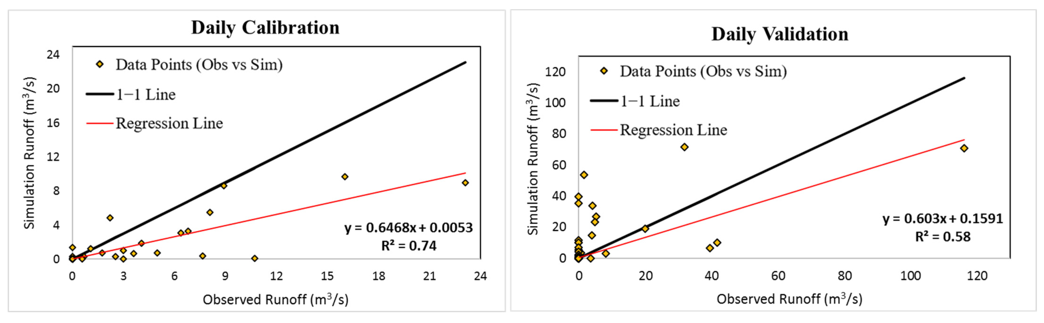
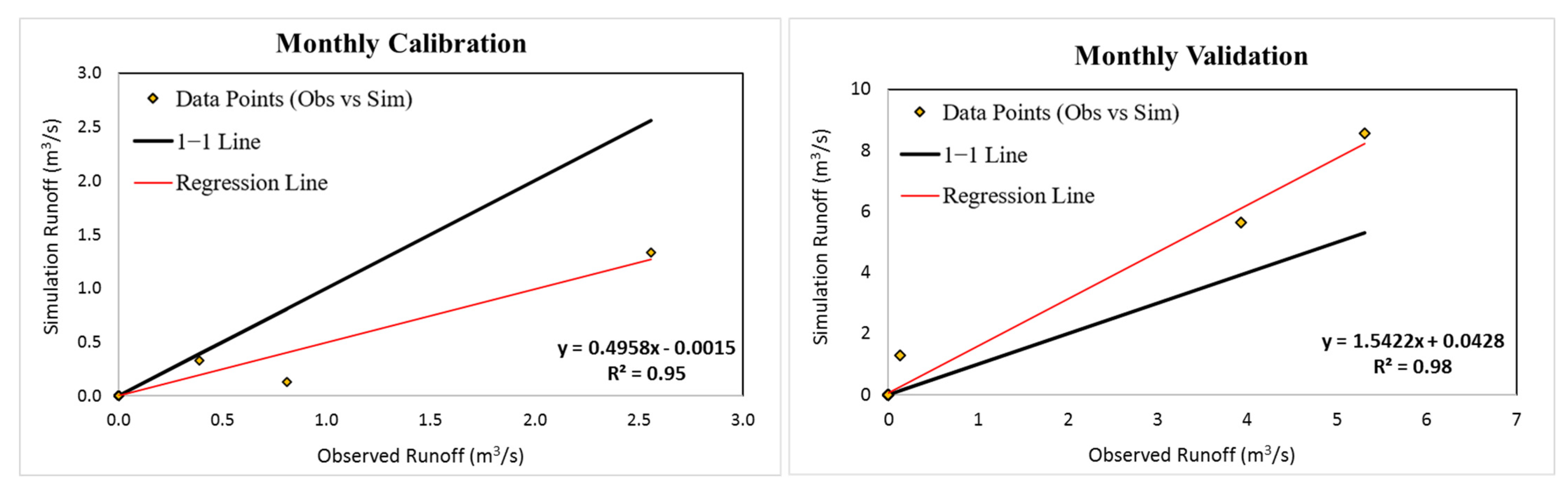
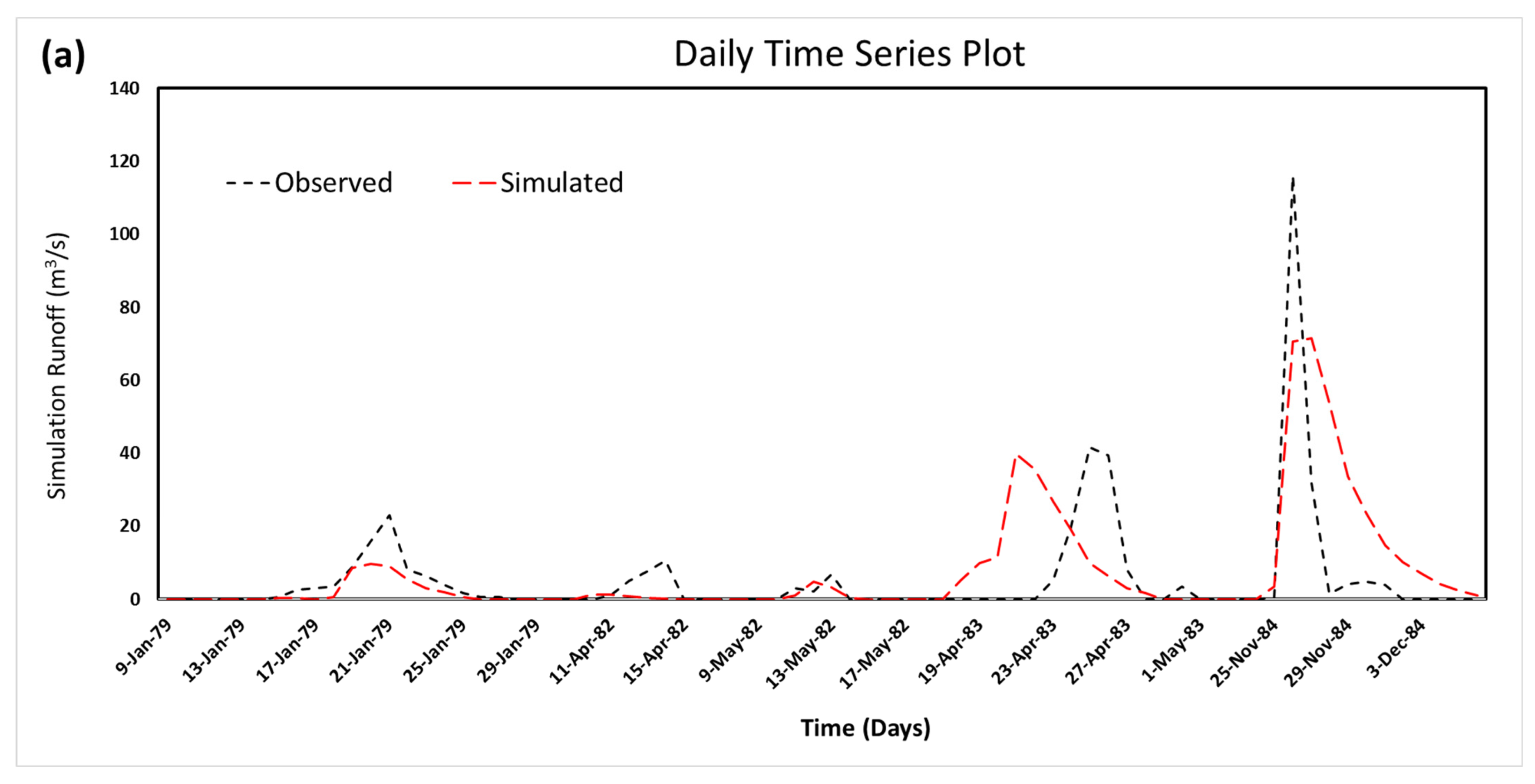
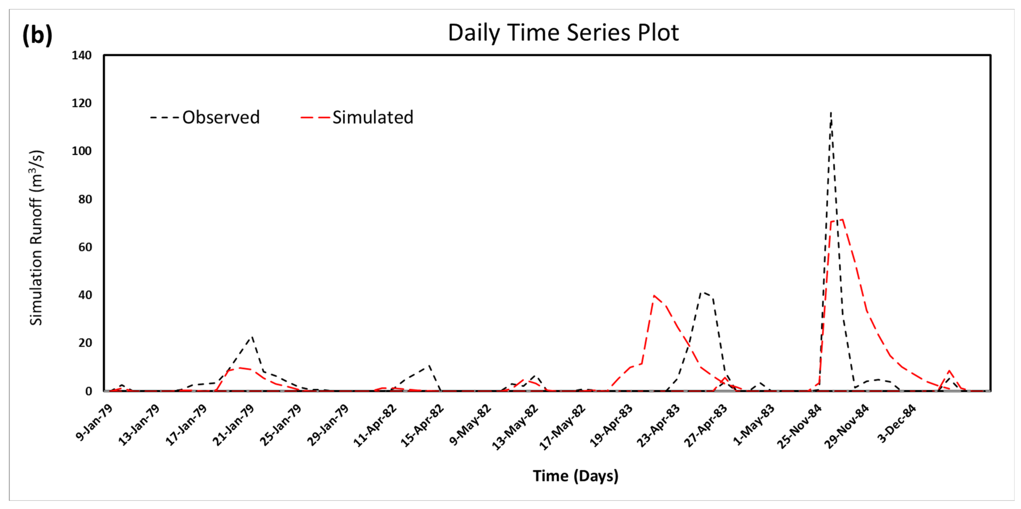
3.1. Model Calibration and Validation

This study was conducted on Wadi Al-Aqul located toward the east of Al-Madinah Al-Munawarah City, in the western part of Saudi Arabia. The study area is considered a hyper-arid region, owing to its very limited rainfall. The observational dataset for runoff is very limited, as the data in it cover a period of only 6 years (1979–1984). The SWAT model was used for the simulation of runoff, while calibration/validation was performed by an integrated model, SWAT-CUP, over a daily and monthly time scale. The first four years (1979–1982) were used as a calibration period, while the next two years (1983–1984) were used as validation. In the calibration period, the model performed well compared to the daily observational runoff, indicating good agreement metrics, including correlation and regression values of 0.86 and 0.74, respectively. The error matrix (MAE and RMSE) presented low values (0.05 and 0.58), while the percent bias (PBIAS) was found to be −54.1%, indicating that the model’s predictions are generally close to the observed values, but some underestimation was found in simulated values. Figure 8 depicts the regression plot between the observed and simulated values for daily time scales’ calibration/validation.
During the validation period, the correlation (regression) 0.76 (0.58) was found to be very high, indicating an excellent extent of agreement between the simulated and observed values for the daily time scale. The PBIAS was 65.7%, indicating overestimation of the simulated values. The daily simulation results can be deemed satisfactory, as per the criteria established by [46].
The fitted parameters estimated in the calibration of daily runoff were implemented to the monthly simulation, which performed excellently for both time spans (calibration/validation). For the monthly calibration period, the model performed better than the daily model response, providing an extremely high correlation coefficient (regression), i.e., 0.97 (0.95), and a very high NS (0.73). The error metrics, MAE and RMSE, were also lower (0.04 and 0.2), with a PBIAS of −52.4%, indicating an underestimation of the model, as found in the daily calibration time span. Similarly, for the validation period, the model had a very good response to the observed values, providing a correlation of 0.99, with regression coefficient of 0.98, thus indicating an extremely high performance. The Nash–Sutcliffe was found to be 0.63, providing a high degree of agreement with overestimation (PBIAS = 65.2) in the simulated values. The MAE and RMSE were 0.25 and 0.78, respectively, slightly higher than calibration, but the overall values remained within an acceptable range. The regression plot for the monthly time scale between the simulated and observed values can be seen in Figure 9.
Both the daily and monthly performance, notably in calibration, highlight the model’s potential for hydrological research in similar strongly arid areas. These findings, regardless of a little tendency toward underestimation and overestimation in the calibration and validation period, respectively, help us to understand the hydrological processes in hyper-arid regions. During extreme events, the peaks of the simulated values for the daily simulation were low as compared to those observed; however, for the monthly simulation, those peaks were overestimated. The reasons for such behavior varies, e.g., model sensitivity toward temporal scales and extremes [50,51]. It also acts as a useful tool for managing and planning water resources in hyper-arid regions, as indicated by statistical measures in Table 6.
The novelty of this research is that, for such a large basin, the fitted parameters of daily calibration can be used perfectly for monthly simulations without further processing being needed for monthly datasets. In contrast, the monthly modeling in this study shows a greater performance in terms of both calibration and validation stages.
The process of aggregating data serves to reduce the impact of random variations, hence improving the model’s capacity to match the simulated values with observed data accurately. The time-series plot of calibration and validation for both time scales can be seen in Figure 10a,b. However, the temporal-scale selection for modeling is generally based on the study’s objective. Monthly modeling is highly effective in capturing the wider patterns and, throughout the year, fluctuations in runoff, demonstrating a stronger correlation with the overall dynamics of hydrological systems. Daily modeling also performed well, indicating that this model can be used for this region at this scale.

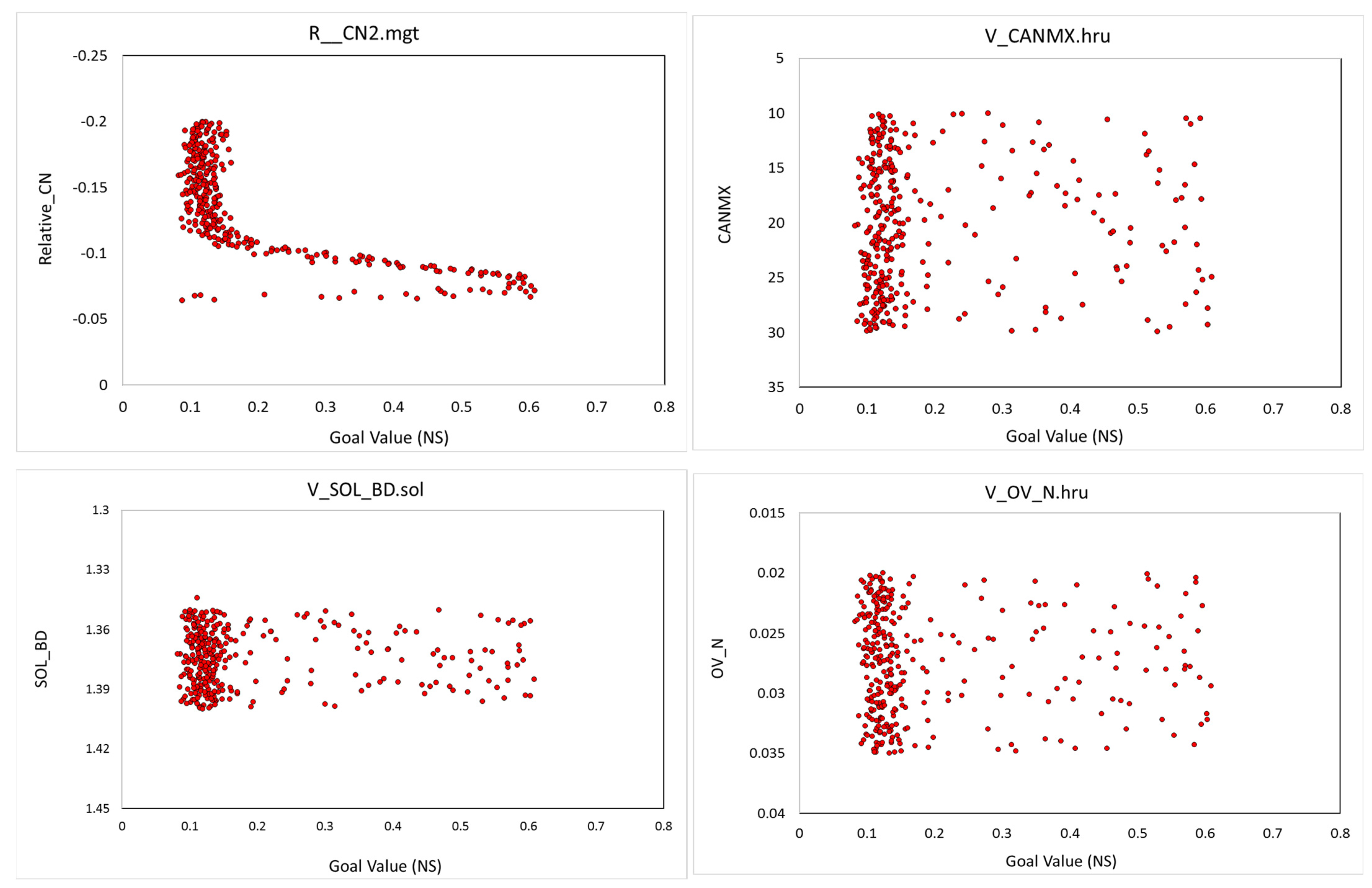
3.2. Sensitivity Analysis

The sensitivity analysis plays a crucial role in identifying the parameters that most significantly influence model outputs, thereby guiding effective calibration and improving model reliability. There are numerous hydrological parameters, but not all of them are sensitive to streamflow, and they vary according to the characteristics of the area. In this study, we conducted a sensitivity analysis to assess the influence of 15 key parameters on the SWAT model’s performance, as measured by the Nash–Sutcliffe efficiency (NS). To perform the sensitivity analysis, the SWAT-CUP tool with the SUFI-2 algorithm was employed, facilitating a comprehensive sensitivity and uncertainty analysis. The existing analysis focused on 15 parameters, which were established by reviewing the literature [52,53,54], and their global sensitivity was assessed for streamflow measurement based on their statistical ranking, upon p- and t-test values, as shown in Figure 11.
For the calibration and uncertainty evaluation, 500 simulations were executed which provided the most sensitive parameters based on their t- and p-test values. In the present study, the Curve Number (CN2) was noted to be the most responsive parameter toward the streamflow, as it is common in strongly arid regions [55,56]. Curve Numbers (CNs) and the number of Hydrological Response Units (HRUs) across the watershed’s sub-basins are crucial for understanding the area’s hydrological characteristics. Collectively, the entire watershed exhibits an average CN of 81, encompassing a total of 121 HRUs. The watershed is divided into five sub-basins, each with a specific Curve Number and a corresponding number of HRUs. Sub-Basin 1 has a CN of 81, with 19 HRUs; Sub-Basin 2 also has a CN of 81, but includes 31 HRUs; and Sub-Basin 3, similarly, has a CN of 81, with 29 HRUs. Sub-Basin 4 shows a slightly lower CN of 80, containing 26 HRUs, while Sub-Basin 5 has a CN of 81, with 16 HRUs. The uniform CN values across most sub-basins suggest consistent runoff potential throughout the watershed, with minor variation observed in Sub-Basin 4. The variation in the number of HRUs among the sub-basins indicates differences in land use and hydrological response within the watershed, as depicted in Figure 4, Figure 5 and Figure 6.
Some parameters, including, GW_Delay, SOL_K (1,3), SOL_K (2,4,5), and SURLAG, were found to be on the least side (p > 0.05) of sensitivity, while SOL_BD, CANMAX, and OV_N were found to be on the moderate side of sensitivity because they have a p-value below 0.05. The uncertainty findings derived from SUFI-2 algorithm indicated the reliability of the SWAT model for modeling large basins. The dotty plots showed the distribution of the number of simulations in the parameter-sensitivity analysis after comparing the parameter values with the objective function (NS) for the calibrations. The uncertainties associated with parameters during streamflow calibration, determined through SUFI-2 techniques, are shown in Table 7.
Figure 12 demonstrates the impact of changing model parameters on NS values. The sensitivity plots generated for each parameter display the relationship between the parameter values and the corresponding NS values, providing insights into the parameters’ influence on model performance. For instance, the most sensitive parameter, CN2, reveals a dense cluster of points around −0.12–0.2 on the y-axis and 0.1–0.2 on the x-axis, indicating a region of high variability in CN but low model performance. However, the points in a specific range (−0.1 to −0.05) have substantial differences in model performance, indicating the high sensitivity of the model’s performance to CN2 variations. This suggests that the precise calibration of CN2 is also critical within this range to achieve reliable model predictions. Likewise, the SOL_BD parameter (soil bulk density) against the Nash–Sutcliffe efficiency (NS) provides insights into how variations in bulk density affect the performance of the model. The dense clustering at lower NS values (0.1 to 0.2) suggests that the model performance is relatively insensitive to variations in SOL_BD within this range. The scattered points at higher NS values (above 0.2) indicate a diverse model performance. In a similar way, the CANMX parameter provides insights into its influence on the model’s performance, as measured by the NS value. The CANMAX plot shows a dense cluster of points at NS values between 0.1 and 0.2, suggesting that the model does not perform well with these parameter settings. However, NS values of beyond 0.2 become more scattered (diverse model performances), suggesting that, for higher NS values, the performance of the model is less sensitive to changes in CANMX. A similar trend of scattering was found in most of the parameters, indicating less sensitivity to the model’s performance.

4. Discussion

The SWAT model is a good tool for hydrological responses estimations, but its implication in strongly arid regions and large watersheds becomes complex due to the unavailability of hydro-climatic data [57,58]. Despite these challenges, findings from the existing study demonstrated that the SWAT model is capable of reliably predicting runoff in hyper-arid regions where data are scarce, as highlighted by [54,59]. The performance of the SWAT model was evaluated on both daily and monthly time scales, indicating a better model performance at the monthly scale compared to the daily in hyper-arid regions, thus resembling the studies of [60,61]. According to [62], the good performance of the monthly time scale in SWAT is due to the data aggregation and less random variations in model simulation, which is in agreement with the findings of [53,58]. Importantly, the model is suitable for capturing broader runoff patterns in arid and hyper-arid regions, making it a valuable tool for climate change studies and long-term water resource management. The sensitivity analysis using the SWAT-CUP tool with the SUFI-2 algorithm was crucial in identifying the parameters that most significantly influence the SWAT model’s performance [51,63]. Among all selected parameters, the curve number (CN2) and soil bulk density (SOL_BD) were identified as the most sensitive parameters, as found by [50,58,64]. Therefore, accurate calibration of CN2 is essential, as small inaccuracies can lead to significant discrepancies in runoff predictions. This finding emphasizes the importance of detailed land cover mapping and soil surveys in hyper-arid regions to improve model accuracy [65,66]. The uncertainty analysis, conducted through 500 simulations, confirmed the relationship between parameter values and the Nash–Sutcliffe efficiency (NS), highlighting areas of high variability and parameter influence.

5. Implications for Hydrological Modeling

The combined findings from the model performance evaluation and sensitivity analysis have several key implications for hydrological modeling in hyper-arid regions:
  • Model calibration and validation: The SWAT model’s ability to simulate runoff on both daily and monthly scales supports its application in hydrological studies and water resource management. The superior performance of the monthly model highlights the benefits of data aggregation in reducing random variations and improving accuracy.
  • Critical parameter identification: The identification of CN2 and SOL_BD as the most sensitive parameters underscores their importance in runoff simulations. The accurate calibration of these parameters is crucial, particularly in hyper-arid regions, where streamflow predictions are highly variable.
  • Model reliability and application: The use of the SWAT-CUP tool with SUFI-2 for the sensitivity and uncertainty analysis proved effective, enhancing the understanding of model behavior. This comprehensive approach ensures more informed calibration and validation, thereby improving model reliability.

6. Limitations and Recommendations

The limitation of this study is data scarcity on the spatiotemporal scale, which is common in hyper-arid regions. Long-term data would enhance the model’s calibration and validation, potentially improving its performance on a daily scale. The rain gauges are also important in this large watershed to capture spatial heterogeneity in the rainfall. A real-time monitoring station must be installed to improve the model’s performance. Despite this limitation, the model performed well on a monthly scale, suggesting its suitability for long-term hydrological studies and climate change-impact assessments.

7. Conclusions

This study provided valuable insights into the modeling of runoff in the challenging hyper-arid region of Wadi Al-Aqul in the western part of Saudi Arabia. Despite the scarcity of observational data, limited to the years 1979–1984, this study successfully tackled the complexities inherent in strongly arid environments. The calibration (1979–1982) and validation period (1983–1984) demonstrated the SWAT model’s capability to simulate daily and monthly runoff with reasonable accuracy. The SWAT model showed a strong performance during the calibration period, with high correlation coefficients (r = 0.86), regression (R2 = 0.76), and Nash–Sutcliffe efficiency (NSE = 0.61), indicating good agreement with observed data. The validation phase maintained a satisfactory performance in regard to the correlation (r = 0.76) and regression (R2 = 0.58). Implementing daily fitted parameters into the monthly simulation emerged as a refined approach, excelling in both the calibration and validation periods. Monthly simulations provided a comprehensive representation of runoff patterns, reducing the impact of random fluctuations and enhancing the model’s accuracy. The significant percent bias (PBIAS) observed during calibration (−54.1%) and validation (65.7%) phases requires thorough model parameter adjustment, but this is restricted with such a limited dataset. However, in such a complex condition, still, it contributes to the satisfactory performance of the model, as highlighted in different studies. The sensitivity analysis identified key parameters influencing streamflow estimation, with the Curve Number (CN) being the most responsive parameter, highlighting the importance of accurate calibration. The study demonstrates the SWAT model’s potential for hydrological research and water resource management in hyper-arid regions, offering a tool for effective planning and management, even with limited data. The findings underscore the model’s utility in long-term climate change-impact assessments, providing a framework for understanding hydrological responses under various climatic scenarios. Future research should focus on enhanced data collection either by installing new gauges or incorporating high-resolution datasets, such as reanalysis data, to overcome data-scarcity issues.

Author Contributions

Conceptualization, S.H., B.N. and A.M.E.; methodology, S.H. and A.M.E.; validation, S.H., B.N., A.M.E., M.M. and X.W.; writing original draft preparation, S.H. and M.A.; review and editing, S.H., B.N., A.M.E., M.M. and X.W. All authors have read and agreed to the published version of the manuscript.

Funding

This research was funded by the Deanship of Scientific Research (DSR), King Abdulaziz University, Jeddah, under Grant No. (IFPRC–017–155–2020).

Data Availability Statement

All data generated or analyzed during this study are included in this published article.

Acknowledgments

The authors extend their appreciation to the Deputyship for Research & Innovation, Ministry of Education in Saudi Arabia for funding this research work through the project number IFPRC–017–155–2020 and King Abdulaziz University, DSR, Jeddah, Saudi Arabia.

Conflicts of Interest

The authors declare no conflicts of interest.

References

  1. Botseva, D.; Tanakov, N.; Nikolov, G. Intelligent Water Resources Management. In Sustainable Development of Water and Environment; Springer: Berlin/Heidelberg, Germany, 2022; pp. 263–273. [Google Scholar]
  2. Li, L.; Zhou, Y.; Li, M.; Cao, K.; Tao, Y.; Liu, Y. Integrated modelling for cropping pattern optimization and planning considering the synergy of water resources-society-economy-ecology-environment system. Agric. Water Manag. 2022, 271, 107808. [Google Scholar] [CrossRef]
  3. Islam, M.; Kashem, S.; Momtaz, Z.; Hasan, M.M. An application of the participatory approach to develop an integrated water resources management (IWRM) system for the drought-affected region of Bangladesh. Heliyon 2023, 9, e14260. [Google Scholar] [CrossRef] [PubMed]
  4. Saeed, E.; Al-Amir, N.; Elfeki, A. Assessment of dams’ efficiency under the effect of climate change and urban expansion: Brayman Dam (Case Study). Res. Sq. 2022. [Google Scholar] [CrossRef]
  5. Kassem, A.A.; Raheem, A.M.; Khidir, K.M.; Alkattan, M. Predicting of daily Khazir basin flow using SWAT and hybrid SWAT-ANN models. Ain Shams Eng. J. 2020, 11, 435–443. [Google Scholar] [CrossRef]
  6. Zakizadeh, H.; Ahmadi, H.; Zehtabian, G.; Moeini, A.; Moghaddamnia, A. A novel study of SWAT and ANN models for runoff simulation with application on dataset of metrological stations. Phys. Chem. Earth Parts A/B/C 2020, 120, 102899. [Google Scholar] [CrossRef]
  7. Javadinejad, S.; Dara, R.; Jafary, F. Analysis and prioritization the effective factors on increasing farmers resilience under climate change and drought. Agric. Res. 2021, 10, 497–513. [Google Scholar] [CrossRef]
  8. Mirramazani, S.M.; Javadinejad, S.; Eslamian, S.; Ostad-Ali-Askari, K. The Origin of River Sediments, the Associated Dust and Climate Change. J. Flood Risk Manag. 2017, 8, 149–172. [Google Scholar]
  9. Yousefi, S.; Pourghasemi, H.R.; Rahmati, O.; Keesstra, S.; Emami, S.N.; Hooke, J. Geomorphological change detection of an urban meander loop caused by an extreme flood using remote sensing and bathymetry measurements (a case study of Karoon River, Iran). J. Hydrol. 2021, 597, 125712. [Google Scholar] [CrossRef]
  10. Azeez, O.; Elfeki, A.; Kamis, A.S.; Chaabani, A. Dam break analysis and flood disaster simulation in arid urban environment: The Um Al-Khair dam case study, Jeddah, Saudi Arabia. Nat. Hazards 2020, 100, 995–1011. [Google Scholar] [CrossRef]
  11. El Bastawesy, M.; Habeebullah, T.; Balkhair, K.; Ascoura, I. Modelling flash floods in arid urbanized areas: Makkah (Saudi Arabia). Sci. Chang. Planétaires/Sécher. 2013, 24, 171–181. [Google Scholar] [CrossRef]
  12. Allam, M.N.; Balkhair, K.S. Case study evaluation of the geomorphologic instantaneous unit hydrograph. Water Resour. Manag. 1987, 1, 267–291. [Google Scholar] [CrossRef]
  13. Li, X.; Long, D.; Slater, L.J.; Moulds, S.; Shahid, M.; Han, P.; Zhao, F. Soil Moisture to Runoff (SM2R): A Data-Driven Model for Runoff Estimation Across Poorly Gauged Asian Water Towers Based on Soil Moisture Dynamics. Water Resour. Res. 2023, 59, e2022WR033597. [Google Scholar] [CrossRef]
  14. Hernández-Bedolla, J.; García-Romero, L.; Franco-Navarro, C.D.; Sánchez-Quispe, S.T.; Domínguez-Sánchez, C. Extreme Runoff Estimation for Ungauged Watersheds Using a New Multisite Multivariate Stochastic Model MASVC. Water 2023, 15, 2994. [Google Scholar] [CrossRef]
  15. Hagras, A. Runoff modeling using SCS-CN and GIS approach in the Tayiba Valley Basin, Abu Zenima area, South-west Sinai, Egypt. Model. Earth Syst. Environ. Res. Lett. 2023, 9, 3883–3895. [Google Scholar] [CrossRef]
  16. Ahmadi, M.; Moeini, A.; Ahmadi, H.; Motamedvaziri, B.; Zehtabiyan, G.R. Comparison of the performance of SWAT, IHACRES and artificial neural networks models in rainfall-runoff simulation (case study: Kan watershed, Iran). Phys. Chem. Earth Parts A/B/C 2019, 111, 65–77. [Google Scholar] [CrossRef]
  17. Noori, N.; Kalin, L. Coupling SWAT and ANN models for enhanced daily streamflow prediction. J. Hydrol. 2016, 533, 141–151. [Google Scholar] [CrossRef]
  18. Grusson, Y.; Anctil, F.; Sauvage, S.; Sánchez Pérez, J.M. Testing the SWAT model with gridded weather data of different spatial resolutions. Water 2017, 9, 54. [Google Scholar] [CrossRef]
  19. Hosseini, M.; Ghafouri, M.; Tabatabaei, Z.; Mokarian, M. Estimation of water balance in watersheds led to west-south frontiers and Persian Gulf by semi distributed SWAT model. J. Water Soil Sci. 2017, 20, Pe183–Pe193. [Google Scholar] [CrossRef]
  20. Valeh, S.; Motamedvairi, B.; Kiadaliri, H.; Ahmadi, H. Hydrological simulation of Ammameh basin by artificial neural network and SWAT models. Phys. Chem. Earth Parts A/B/C 2021, 123, 103014. [Google Scholar] [CrossRef]
  21. Rocha, A.K.P.; de Souza, L.S.B.; de Assunção Montenegro, A.A.; de Souza, W.M.; da Silva, T.G.F. Revisiting the application of the SWAT model in arid and semi-arid regions: A selection from 2009 to 2022. Theor. Appl. Climatol. 2023, 154, 7–27. [Google Scholar] [CrossRef]
  22. Pandi, D.; Kothandaraman, S.; Kuppusamy, M. Simulation of water balance components using SWAT model at sub catchment level. Sustainability 2023, 15, 1438. [Google Scholar] [CrossRef]
  23. Diriba, B.T. Surface runoff modeling using SWAT analysis in Dabus watershed, Ethiopia. Sustain. Water Resour. Manag. 2021, 7, 96. [Google Scholar] [CrossRef]
  24. Marahatta, S.; Devkota, L.P.; Aryal, D. Application of SWAT in hydrological simulation of complex Mountainous river basin (part I: Model development). Water 2021, 13, 1546. [Google Scholar] [CrossRef]
  25. Tibebe, D.; Bewket, W. Surface runoff and soil erosion estimation using the SWAT model in the Keleta watershed, Ethiopia. Land Degrad. Dev. 2011, 22, 551–564. [Google Scholar] [CrossRef]
  26. Zhihua, L.; Zuo, J.; Rodriguez, D. Predicting of runoff using an optimized SWAT-ANN: A case study. J. Hydrol. Reg. Stud. 2020, 29, 100688. [Google Scholar]
  27. Thavhana, M.; Savage, M.; Moeletsi, M. SWAT model uncertainty analysis, calibration and validation for runoff simulation in the Luvuvhu River catchment, South Africa. Phys. Chem. Earth Parts A/B/C 2018, 105, 115–124. [Google Scholar] [CrossRef]
  28. Ezz-Aldeen, M.; Al-Ansari, N.; Knutsson, S. Application of SWAT model to estimate the runoff and sediment load from the Right Bank Valleys of Mosul Dam Reservoir. In Proceedings of the International Conference on Scour and Erosion, Paris, France, 27–31 August 2012. [Google Scholar]
  29. Eugster, W.; Erik, J.S.; Brian, F. Wind Effects, Encyclopedia of Ecology; Academic Press: Oxford, UK, 2008. [Google Scholar]
  30. Niyazi, B.; Masoud, M.; Elfeki, A.; Rajmohan, N.; Alqarawy, A.; Rashed, M. A Comparative Analysis of Infiltration Models for Groundwater Recharge from Ephemeral Stream Beds: A Case Study in Al Madinah Al Munawarah Province, Saudi Arabia. Water 2022, 14, 1686. [Google Scholar] [CrossRef]
  31. Das, M.; Hazra, A.; Sarkar, A.; Bhattacharya, S.; Banik, P. Comparison of spatial interpolation methods for estimation of weekly rainfall in West Bengal, India. Mausam 2017, 68, 41–50. [Google Scholar] [CrossRef]
  32. Chutsagulprom, N.; Chaisee, K.; Wongsaijai, B.; Inkeaw, P.; Oonariya, C.J.T.; Climatology, A. Spatial interpolation methods for estimating monthly rainfall distribution in Thailand. Theor. Appl. Climatol. 2022, 148, 317–328. [Google Scholar] [CrossRef]
  33. Al-Saady, Y.; Merkel, B.; Al-Tawash, B.; Al-Suhail, Q. Land use and land cover (LULC) mapping and change detection in the Little Zab River Basin (LZRB), Kurdistan Region, NE Iraq and NW Iran. FOG-Freib. Online Geosci. 2015, 43. Available online: https://www.academia.edu/20211670/Land_use_and_land_cover_LULC_mapping_and_change_detection_in_the_Little_Zab_River_Basin_LZRB_Kurdistan_Region_NE_Iraq_and_NW_Iran (accessed on 15 June 2024).
  34. da Silva, V.S.; Salami, G.; da Silva, M.I.O.; Silva, E.A.; Monteiro Junior, J.J.; Alba, E. Methodological evaluation of vegetation indexes in land use and land cover (LULC) classification. Geol. Ecol. Landsc. 2020, 4, 159–169. [Google Scholar] [CrossRef]
  35. Satapathy, A.; Naik, B.; Awasthi, N.; Kaushik, V. Estimation of Surface Runoff Using SWAT Model and ArcGIS Approach. Int. J. COMADEM 2023, 26, 37. [Google Scholar]
  36. Alawi, S.A.; Özkul, S. Evaluation of land use/land cover datasets in hydrological modelling using the SWAT model. H2Open J. 2023, 6, 63–74. [Google Scholar] [CrossRef]
  37. Shukla, S.; Meshesha, T.W.; Sen, I.S.; Bol, R.; Bogena, H.; Wang, J. Assessing Impacts of Land Use and Land Cover (LULC) Change on Stream Flow and Runoff in Rur Basin, Germany. Sustainability 2023, 15, 9811. [Google Scholar] [CrossRef]
  38. Saxton, K.E.; Willey, P.H. The SPAW model for agricultural field and pond hydrologic simulation. In Watershed Models; CRC Press: Boca Raton, FL, USA, 2006; pp. 401–435. [Google Scholar]
  39. Winchell, M.; Srinivasan, R.; Di Luzio, M.; Arnold, J. ArcSWAT Interface for SWAT2012: User’s Guide. Blackland Research and Extension Center, Texas Agrilife Research. Grassland; Soil Water Research Laboratory, USDA Agricultural Research Service: Temple, TX, USA, 2013; Volume 3, p. 464. [Google Scholar]
  40. Pignotti, G.; Rathjens, H.; Cibin, R.; Chaubey, I.; Crawford, M. Comparative analysis of HRU and grid-based SWAT models. Water 2017, 9, 272. [Google Scholar] [CrossRef]
  41. Arnold, J.; Kiniry, J.; Srinivasan, R.; Williams, J.; Haney, E.; Neitsch, S. SWAT Input/Output Documentation Version; Texas Water Resources Institute: College Station, TX, USA, 2012; Volume 654, pp. 1–646. [Google Scholar]
  42. Saha, A.K.; McMaine, J. Applicability and sensitivity of field hydrology modeling by the Soil Plant Air Water (SPAW) model under changes in soil properties. J. ASABE 2023, 66, 809–823. [Google Scholar] [CrossRef]
  43. Arnold, J.; Kiniry, J.; Srinivasan, R.; Williams, J.; Haney, E.; Neitsch, S. Soil and Water Assessment Tool Input/Output File Documentation Version 2009; Texas Water Resources Institute: College Station, TX, USA, 2011. [Google Scholar]
  44. Abbaspour, K.; Calibration, S. Uncertainty Programs—A User Manual; Swiss Federal Institute of Aquatic Science and Technology: Duebendorf, Switzerland, 2008; 95p. [Google Scholar]
  45. Abbaspour, K.C.; Johnson, C.; Van Genuchten, M.T. Estimating uncertain flow and transport parameters using a sequential uncertainty fitting procedure. Vadose Zone J. 2004, 3, 1340–1352. [Google Scholar] [CrossRef]
  46. Moriasi, D.N.; Arnold, J.G.; Van Liew, M.W.; Bingner, R.L.; Harmel, R.D.; Veith, T.L. Model evaluation guidelines for systematic quantification of accuracy in watershed simulations. Trans. ASABE 2007, 50, 885–900. [Google Scholar] [CrossRef]
  47. Jimeno-Sáez, P.; Senent-Aparicio, J.; Pérez-Sánchez, J.; Pulido-Velazquez, D. A comparison of SWAT and ANN models for daily runoff simulation in different climatic zones of peninsular Spain. Water 2018, 10, 192. [Google Scholar] [CrossRef]
  48. Schaefli, B.; Gupta, H.V. Do Nash values have value? Hydrol. Process. 2007, 21, 2075–2080. [Google Scholar] [CrossRef]
  49. Su, Q.; Dai, C.; Zhang, Z.; Zhang, S.; Li, R.; Qi, P. Runoff Simulation and Climate Change Analysis in Hulan River Basin Based on SWAT Model. Water 2023, 15, 2845. [Google Scholar] [CrossRef]
  50. Singh, A.; Jha, S.K. Identification of sensitive parameters in daily and monthly hydrological simulations in small to large catchments in Central India. J. Hydrol. 2021, 601, 126632. [Google Scholar] [CrossRef]
  51. Li, M.; Di, Z.; Duan, Q. Effect of sensitivity analysis on parameter optimization: Case study based on streamflow simulations using the SWAT model in China. J. Hydrol. 2021, 603, 126896. [Google Scholar] [CrossRef]
  52. Sahu, M.; Lahari, S.; Gosain, A.; Ohri, A. Hydrological modeling of Mahi basin using SWAT. J. Water Resour. Hydraul. Eng. 2016, 5, 68–79. [Google Scholar] [CrossRef]
  53. Carlos Mendoza, J.A.; Chavez Alcazar, T.A.; Zuñiga Medina, S.A. Calibration and uncertainty analysis for modelling runoff in the Tambo River Basin, Peru, using Sequential Uncertainty Fitting Ver-2 (SUFI-2) algorithm. Air Soil Water Res. 2021, 14, 1178622120988707. [Google Scholar] [CrossRef]
  54. Hosseini, S.H.; Khaleghi, M.R. Application of SWAT model and SWAT-CUP software in simulation and analysis of sediment uncertainty in arid and semi-arid watersheds (case study: The Zoshk–Abardeh watershed). Model. Earth Syst. Environ. 2020, 6, 2003–2013. [Google Scholar] [CrossRef]
  55. Farhan, A.M.; Al Thamiry, H.A. Estimation of the surface runoff volume of Al-Mohammedi valley for long-term period using SWAT model. Iraqi J. Civ. Eng. 2022, 14, 7–12. [Google Scholar]
  56. Khatun, S.; Sahana, M.; Jain, S.K.; Jain, N. Simulation of surface runoff using semi distributed hydrological model for a part of Satluj Basin: Parameterization and global sensitivity analysis using SWAT CUP. Model. Earth Syst. Environ. 2018, 4, 1111–1124. [Google Scholar] [CrossRef]
  57. Mengistu, A.G.; van Rensburg, L.D.; Woyessa, Y.E. Techniques for calibration and validation of SWAT model in data scarce arid and semi-arid catchments in South Africa. J. Hydrol. Reg. Stud. 2019, 25, 100621. [Google Scholar] [CrossRef]
  58. Abu-Zreig, M.; Hani, L.B. Assessment of the SWAT model in simulating watersheds in arid regions: Case study of the Yarmouk River Basin (Jordan). Open Geosci. 2021, 13, 377–389. [Google Scholar] [CrossRef]
  59. Nasiri, S.; Ansari, H.; Ziaei, A.N. Simulation of water balance equation components using SWAT model in Samalqan Watershed (Iran). Arab. J. Geosci. 2020, 13, 421. [Google Scholar] [CrossRef]
  60. Pang, J.; Zhang, H.; Xu, Q.; Wang, Y.; Wang, Y.; Zhang, O.; Hao, J. Hydrological evaluation of open-access precipitation data using SWAT at multiple temporal and spatial scales. Hydrol. Earth Syst. Sci. 2020, 24, 3603–3626. [Google Scholar] [CrossRef]
  61. Tani, H.; Tayfur, G. Modelling Rainfall-Runoff Process of Kabul River Basin in Afghanistan Using ArcSWAT Model. J. Civ. Eng. Constr. 2023, 12, 1–18. [Google Scholar] [CrossRef]
  62. Castellanos-Osorio, G.; López-Ballesteros, A.; Pérez-Sánchez, J.; Senent-Aparicio, J. Disaggregated monthly SWAT+ model versus daily SWAT+ model for estimating environmental flows in Peninsular Spain. J. Hydrol. 2023, 623, 129837. [Google Scholar] [CrossRef]
  63. Brouziyne, Y.; Abouabdillah, A.; Bouabid, R.; Benaabidate, L.; Oueslati, O. SWAT manual calibration and parameters sensitivity analysis in a semi-arid watershed in North-western Morocco. Arab. J. Geosci. 2017, 10, 427. [Google Scholar] [CrossRef]
  64. Martínez-Salvador, A.; Conesa-García, C. Suitability of the SWAT model for simulating water discharge and sediment load in a karst watershed of the semiarid Mediterranean basin. Water Resour. Manag. 2020, 34, 785–802. [Google Scholar] [CrossRef]
  65. Mehta, D.; Hadvani, J.; Kanthariya, D.; Sonawala, P. Effect of land use land cover change on runoff characteristics using curve number: A GIS and remote sensing approach. Int. J. Hydrol. Sci. Technol. 2023, 16, 1–16. [Google Scholar] [CrossRef]
  66. Gunjan, P.; Mishra, S.K.; Lohani, A.K.; Chandniha, S.K. Impact estimation of landuse/land cover changes and role of hydrological response unit in hydrological modelling in a watershed of Mahanadi river basin, India. Nat. Hazards 2023, 119, 1399–1420. [Google Scholar] [CrossRef]
Figure 1. Study area map of Wadi Al-Aqul, located in Al-Madinah Al-Munawarah Province.
Water 16 02043 g001
Figure 2. Rainfall hyetograph and runoff hydrograph of observed events during study period.
Water 16 02043 g002
Figure 3. Digital Elevation Model with stream network of Wadi Al-Aqul.
Water 16 02043 g003
Figure 4. LULC classification of the Wadi Al-Aqul.
Water 16 02043 g004
Figure 5. FAO soil map of Wadi Al-Aqul.
Water 16 02043 g005
Figure 6. Slope classification of Wadi Al-Aqul.
Water 16 02043 g006
Figure 7. Methodological framework of SWAT modeling.
Water 16 02043 g007
Figure 8. Regression plot between simulated and observed runoff for daily calibration (left) and validation (right).
Water 16 02043 g008
Figure 9. Regression plot between simulated and observed runoff for monthly calibration (left) and validation (right).
Water 16 02043 g009
Figure 10. (a) Observed (dotted black line) and simulated (dotted red line) hydrograph for calibration and validation period of Wadi Al-Aqul on the daily time scale. (b) Monthly calibration/validation in lower panel, indicating observed (dotted black line) and simulated (dotted red line) hydrograph for Wadi Al-Aqul.
Water 16 02043 g010aWater 16 02043 g010b
Figure 11. Radar diagram of sensitivity analysis; p-test on left and t-test (absolute values) on right.
Water 16 02043 g011
Figure 12. Sequential Uncertainty Fitting version 2 (SUFI-2) results for the value of Nash–Sutcliffe vs. parameters value.
Water 16 02043 g012aWater 16 02043 g012bWater 16 02043 g012c
Table 1. Land-use/land-cover types, occupying area, and percent cover.
IndexLULC CodeLand TypeArea in km2Area in %
1BARRBare Soil35,298.199.20
2URHDBuilt-up220.20.62
3AGRRAgriculture65.30.18
4WATRWater0.40.00
Total 35,584100
Table 2. Soil groups.
IndexSoils CodeSoil Area (%)Soil Type
1I-Yk-2ab-313526.6Loam
2I-Y-bc-35154.2Loam
3I-Yh-Yk-1-351846.3Loam
4Yh3-1-2a-358515.5Sandy Loam
5Yk28-1a-35957.4Sandy Loam
Table 3. SWAT-CUP model calibration parameters with range and fitted values.
IndexParameter_NameAbbreviationExtensionFitted_ValueMin_ValueMax_Value
1CN2Curve Number.mgt−0.076−0.100.02
2CH_N2Channel Manning Coefficient.rte0.0320.020.04
3SOL_K (1,3),Soil Hydraulic Conductivity.sol11.1897.0015.00
4SOL_K (2,4,5)Soil Hydraulic Conductivity.sol4.53.006.00
5OV_NOver Land Flow manning.hru0.030.020.04
6MSK_CO1Muskingum Coefficient 1.bsn4.0350.0010.00
7MSK_CO2Muskingum Coefficient 2.bsn2.3710.0010.00
8MSK_XMuskingum Weighting factor.bsn0.0870.000.30
9ALPHA_BFBase Flow.gw0.840.001.00
10SURLAGSurface Lag.bsn15.5121.0024.00
11GW_DELAYGround Water Delay.gw291.962100.00500.00
12SOL_BDSoil Bulk Density.sol1.4651.351.50
13CH_S2Channel Slope.rte0.0050.000.01
14HRU_SLPAverage slope steepness.hru0.0090.000.01
15CANMXMaximum Canopy.hru30.15210.0035.00
Table 4. Evaluation model criteria.
Performance RatingNSEPBIAS (%)
Very goodNSE ≥ 0.7|PBIAS| ≤ 25
Good0.5 ≤ NSE < 0.725 < |PBIAS| ≤ 50
Satisfactory0.3 ≤ NSE < 0.550 < |PBIAS| ≤ 70
UnsatisfactoryNSE < 0.3|PBIAS| > 70
Table 5. Statistical parameters.
NameEquationUsage
Percent bias (PBIAS) i = 1 n ( X i Y i ) i = 1 n X i × 100 Over- and underestimation of the model values
Pearson Correlation Coefficient (r) i = 1 n X i X ¯   ( Y i Y ¯ ) i = 1 n   ( X i X ¯ ) 2   i = 1 n   ( Y i   Y ¯ ) 2 Describe the extent of agreement between observed and simulated runoff
Determination Coefficient (R2) 1 S S r S S T
Nash–Sutcliffe coefficient (NSE) 1 i = 1 n   ( X i Y i ) 2 i = 1 n ( X i X ¯ ) 2  
Root Mean Square Error (RMSE) 1 n i = 1 n ( X i Y i ) 2 Express error between observed and simulated runoff
Mean Absolute Error (MAE) 1 n i = 1 n X i Y i
Notes: Xi is the observed dataset values, Yi is the modeled dataset values, X ¯ is the mean of the observed dataset, Y ¯ is the mean of estimated dataset, n is sample size, SSr is residuals sum of square, and SST is total sum of square.
Table 6. Statistical parameters results.
Daily Monthly
Evaluation ParametersCalibrationValidationCalibrationValidation
r0.860.760.970.99
R20.740.580.950.98
NS0.610.580.730.63
MAE0.050.580.040.25
RMSE0.584.310.200.78
PBIAS−54.165.7−52.465.2
Table 7. Parameter uncertainties during streamflow calibration on a daily basis.
RankParameterTpExt
1CN2−15.700.00mgt
2SOL_BD2.780.01sol
3CANMX2.590.01hru
4OV_N2.000.05hru
5HRU_SLP1.690.09hru
6MSK_CO1−1.580.11bsn
7ALPHA_BF1.280.20gw
8MSK_X−0.750.46bsn
9CH_S2−0.700.48rte
10CH_N20.590.56rte
11MSK_CO20.550.58bsn
12SOL_K(2,4,5)0.450.65sol
13SURLAG−0.300.77bsn
14SOL_K(1,3)−0.150.88sol
15GW_DELAY−0.070.94gw
Disclaimer/Publisher’s Note: The statements, opinions and data contained in all publications are solely those of the individual author(s) and contributor(s) and not of MDPI and/or the editor(s). MDPI and/or the editor(s) disclaim responsibility for any injury to people or property resulting from any ideas, methods, instructions or products referred to in the content.

