Abstract
Saltwater intrusion is an essential problem in estuaries that can threaten the ecological environment, especially in high-salinity situations. Therefore in this paper, traditional multiple linear regression (MLR) and artificial neural network (ANN) modeling are applied to forecast overall and high salinity in the Lower Scheldt Estuary, Belgium. Mutual information (MI) and conditional mutual information (CMI) are used to select optimal driving forces (DFs), with the daily discharge (Q), daily water temperature (WT), and daily sea level (SL) selected as the main DFs. Next, we analyze whether applying a discrete wavelet transform (DWT) to remove the noise from the original time series improves the results. Here, the DWT is applied in Signal-hybrid (SH) and Within-hybrid (WH) frameworks. Both the MLR and ANN models demonstrate satisfactory performance in daily overall salinity simulation over the Scheldt Estuary. The relatively complex ANN models outperform MLR because of their capabilities of capturing complex interactions. Because the nonlinear relationship between salinity and DFs is variable at different locations, the performance of the MLR models in the midstream region is far inferior to that in the downstream region during spring and winter. The results reveal that the application of DWT enhances simulation of both overall and high salinity in this region, especially for the ANN model with the WH framework. With the effect of Q decline or SL rise, the salinity in the middle Scheldt Estuary increases more significantly, and the ANN models are more sensitive to these perturbations.
1. Introduction
As transition zones between the river and the sea, estuaries are particularly vulnerable to saltwater intrusions [1]. Many aquatic organisms are adapted to a specific salinity range, making these ecosystems highly sensitive to salinity changes. The high variety in the estuarine environment presents challenges to the physiology of organisms, with different aquatic communities divided along salinity gradients [2]. In recent years, intensive human activities such as damming and urbanization have significantly changed the natural pattern of the coastal areas and further influenced the ecological environment [3]. In addition, global sea levels are rising at an unprecedented rate due to human-caused global warming. This not only brings coastal flood damages but also intensifies saltwater intrusion [4]. Therefore, long-term accurate and reliable overall and extreme salinity estimations are important and necessary for identifying the general characteristics of salinity and mitigating the negative influences of saltwater intrusion in estuaries.
Two popular approaches could be adopted for salinity modeling, namely, numerical hydrodynamic models, in which the main physical processes are considered (e.g., [5,6]), and data-driven (DD) models, in which empirical observations are used to identify the relations between salinity and the main driving forces (DFs) (e.g., [3,7]). Numerical hydrodynamic models allow for exploration of the hydrodynamic mechanisms of saltwater intrusion, and have obtained desirable results. However, they are computationally intensive and require many different types of field data along with considerable effort to calibrate the model parameters [8]. As an alternative, a DD model with a shorter calculation time and requires fewer information requirements could be developed. Unlike physical or deterministic models, which are based on the underlying physical principles and equations governing the hydrological processes, DD models derive patterns and relationships directly from the data without explicit incorporation of the underlying physical principles [1].
To develop a DD model, sufficient empirical observations that cover the spatial and temporal variations of the salinity are needed. Establishing an appropriate initial pool of DFs is the fundamental basis for achieving a dependable outcome [8]. This initial set of DFs can be determined by considering prior knowledge of saltwater conditions, data availability, and their relevance to the specific study area [9]. The dispersion process of salinity, where tidal surges drive saltwater into the estuary, resulting in increased salinity, can be influenced by a series of factors [7,10,11], while freshwater inflows can dilute the salinity in the estuary [7,12]. Within the estuary, these salinity concentrations are highly varied depending on the tidal movement from the sea (e.g., sea level, tidal range) [13], the upstream freshwater inflows [14], the location, and some other factors [15]. Taking into account previous research experience [1,13] and the geographical and hydrological characteristics of the Scheldt Estuary [16], five variables are considered as the potential DFs: discharge (Q), water temperature (WT), sea level (SL), wind speed (WS), and air temperature above 1.5 m (AT).
Traditional DD models offer simplicity and interpretability, while machine learning models provide flexibility, scalability, and the ability to capture complex relationships [17]. The choice between these approaches depends on the specific requirements of the hydrological problem at hand, including the complexity of the system, available data, computational resources, and need for interoperability. As a traditional statistical methodology, multiple linear regression (MLR) can be used to simulate the salinity condition based on regression relations with multiple DFs. However, numerous studies have shown that the relations between salinity and the DFs are highly complex and typically nonlinear [3,18]. To alleviate this problem, various basic data preprocessing methods (e.g., exponential transform, Box-Cox transform) have been introduced before building the MLR model. Exponential and power-law regression equations were applied to analyze the discharge–salinity relationships in the Pearl River estuary, achieving desirable results [12]. Considering that salinity diffusion is a temporally and spatially continuous physical hydrological process, a process-based empirical model was built using the moving average flow for salinity management in the upper Delaware Estuary [19]. The above examples show that simple data preprocessing can greatly improve simple empirical models at low cost. In this study, the natural log transformation and forward moving average methods are applied to Q for data preprocessing.
In a different approach, machine learning allows higher-order nonlinear fitting, and is known for its efficiency when learning from data with minimal human intervention. Many researchers have used machine learning to model nonlinear hydrological processes over the past decades. In [20], four machine learning algorithms were used to predict the location and extent of salt-influenced areas, including decision tree, k-nearest neighbor, random forest, and support vector machine. In [21], an analysis with a feed-forward artificial neural network (ANN) model with quick propagation was carried out under different pumping frequencies to forecast the groundwater salinity.
One of the main problems in using these DD approaches is the presence of data noise from inputs [17]. To remove noise, several methods are already available, such as the discrete wavelet transform (DWT) [22], empirical mode decomposition [3], and empirical orthogonal function analysis [11]. The popularity of DWT-based approaches stems from their capacity to concurrently reveal both spectral and temporal information within a signal [23]. As an advanced preprocessing technique, the DWT offers valuable decompositions of primary time series, enhancing the model’s efficacy by capturing pertinent information across different resolution levels and providing a more coherent structure [24]. Recently, the DWT has been widely used in conjunction with ANNs and other machine learning algorithms for hydrological and water resource forecasting [25,26]. There are two frameworks for coupling DWT in DD models; one is the ‘Single-hybrid’ (SH) framework, where only the DFs are decomposed, and the other is the ‘Within-hybrid’ (WH) framework, where both the target and DFs are decomposed [27].
To date, most studies have considered advanced decomposition methods in combination with machine learning models instead of traditional statistical models [28,29,30]. Simultaneously, numerous studies have solely relied on overall salinity as the final indicator [3,31], overlooking extremely high salinity values. However, high salinity levels are one of the main factors that most strongly influence the survival of aquatic organisms and surrounding environments [32]. Therefore, in this paper an advanced DWT approach is used in combination with both statistical and machine learning methods to assess both overall salinity and high salinity. In total, six DD models for salinity simulation are developed and systematically compared, including MLR, ANN, MLR-DWT with the SH and WH frameworks, and ANN-DWT with the SH and WH frameworks. This analysis aims to discern the strengths and weaknesses of each model, offering valuable insights for selecting appropriate models in similar studies. The most important DFs are selected, six models are constructed, and then the performance regarding overall and high salinity levels is discussed. Lastly, the models’ structural reliability is verified through sensitivity analyses.
2. Study Area and Data
2.1. Study Area
The Scheldt estuary, located in Belgium, was chosen for a case study. The international Scheldt River originates in the north of France and flows through western Belgium and the southwestern part of The Netherlands to the North Sea (see Figure 1). The river is rain-fed by a catchment of approximately 21.863 km2, and can be divided into the non-tidal Upper Scheldt and the tidally influenced part, which extends from its mouth to the weirs/sluices in Ghent. As a macrotidal and relatively turbid estuary, its mean depth varies from about 14 m at the mouth to 7 m near Gent. The tidal wave also enters the major branches, providing the estuary with approximately 235 km of tidal river. The Belgian part of the estuary (105 km) forms a single tidal channel, which is bordered by relatively small mudflats and marshes [16]. In this study, only the Lower Scheldt estuary is considered due to data availability.
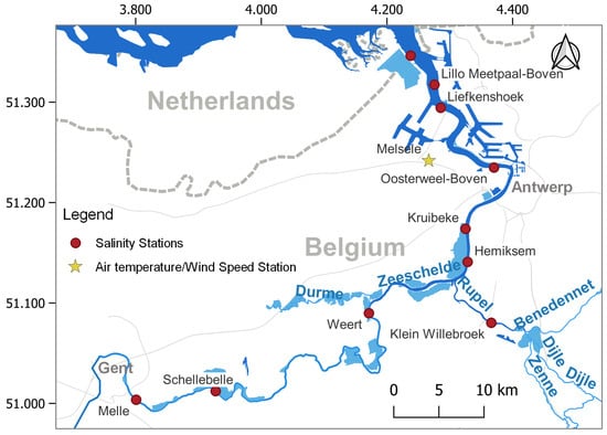
Figure 1.
The Scheldt Estuary and locations of meteorological and salinity stations.
With the transition between fresh and salt water being particularly variable, the salinity intrusion limit migrates along the river [33]. A polyhaline zone and a mesohaline zone in turn extend from the North Sea to the Dutch/Belgian border. The section between the border and Antwerp is characterized by a steep salinity gradient [16]. Upstream of Gent belongs to the freshwater tidal zone, where the salinity varies between 0 and 0.5 psu.
2.2. Data
Publicly available data (https://www.waterinfo.be/ accessed on 5 December 2023) of Salinity, Q, SL, WT, AT, and WS were collected in this study. There are ten stations available for Salinity and WT, of which nine are distributed along the main river and the other is located along the tributary Rupel. Table 1 provides an overview of all stations and their statistical characteristics with regard to salinity. It can be seen that the daily average salinity decreases from outlet to inland. In this area, only one Q station exists, ‘Melle’ (also S station), which is located around 99.3 km upstream of the outlet. For better simulations, a nonparametric DD approach was used to obtain estimations of the river discharges at the Salinity stations [34] by applying interpolation based on the contributing runoff area. The SL refers to the daily water level observed at the downstream ‘Prosperpolder’ station. The WS and AT station ‘Melsele’ is located near Antwerp.

Table 1.
Overview of salinity stations and statistical characteristics in the Scheldt River Estuary.
Considering that Flanders has experienced several droughts over the period from 2018–2020, which can intensify the saltwater intrusion problem due to increased evaporation [35], the study period was chosen from 2016 to 2022. To ensure structural validity, a similar data splitting scheme was applied; a random 70% data subset was selected for calibration and the rest was used for validation. The chosen calibration data for each station remained constant during the entire model calibration process.
3. Methods
3.1. Selection of Driving Forces
By applying appropriate data preprocessing techniques, the dataset can be made more suitable for calibration. This helps to ensure optimal performance and generalizability of DD models, which needs to be carried out prior to the selection. Natural log transformation can help to normalize the distribution of Q, which occurs in the first step. An X-day average moving Q, where the initial X ranges from 1 to 100, is applied to build the relation between its changes with salt intrusion [36].
The dependency between two factors is measured by the Mutual information (MI), and mutual information conditioned on a given factor is calculated using the conditional mutual information (CMI) [37]. These two filters, MI and CMI, have been widely used for uncertainty analysis in hydrology [27,38]. In this study, the initial DFs are Q, WT, SL, WS, and AT. Considering the independence from and coupling ability with regression models, these ‘filter’ algorithms are adopted to choose the final optimal DFs [9]. The MI of X and Y is provided as follows [29]:
where the entropy is an estimate of the uncertainty of the random variable X. The conditional entropy indicates the remaining uncertainty of X after Y is known. A high value means that X and Y are highly related, and vice versa.
To overcome the potential problem of redundancy and conditional irrelevance, one (a group of) other factor is set as condition(s) to calculate the CMI during selection [39]. The CMI between X and Y conditioned on Z is provided as follows [29]:
where equals when Y and Z have same information and is non-negative. In this study, the first DF and the corresponding optimal moving average days are selected based on the highest MI. Afterwards, CMI is applied to select the other DFs. The specific procedures for computing the MI and CMI are as outlined in previous studies [1,40].
3.2. Multiple Linear Regression (MLR)
MLR is a statistical methodology employed to leverage a collection of explanatory variables for simulating the outcome of a response variable. The fundamental objective underlying MLR is the modeling of linear associations between explanatory variables, which are independent in nature, and the response variable, which is dependent. The equation can be represented as follows [24]:
where Y is the target object, to represent all external DFs, to are their corresponding regression slopes, and is the intercept. The coefficients are determined using the least squares method. To account for the nonlinear relationship between salinity and the DFs, a natural logarithmic transformation is applied to the DFs.
3.3. Artificial Neural Network (ANN)
ANNs offer several advantages, including the ability to function effectively with modest data prerequisites, rapid computational execution, and the capacity to generate models that elucidate complex input–output relationships [25]. The multilayer perceptron (MLP) network, featuring a feedforward back-propagation (BP) network structure, represents a widely utilized paradigm in water science applications [28]. An ordinary ANN typically comprises three layers: the input layer, the output layer, and one or more hidden layers. The input is linked to the neurons in the intermediate layer through varying weights, then these intermediate neurons are further linked to the output layer through varying weights. More details about the MLP network can be found in [41]. ANN models with only one hidden layer have proven to be sufficient for hydrology applications [1]. Therefore, in this study we selected a three-layer BP model structure after comprehensive consideration of accuracy and computational time cost.
Standard neural network training methods involve modifying the weights and biases within the network to reduce a measure of ’error’ in the training samples, typically characterized as the sum of squared variances between the network predictions and the desired target values [41]. The logistic sigmoid activation function is chosen to calculate the output of each neuron in the hidden layer, while the linear activation function is used for the output layer. As one of the fastest methods for training ANN models, the Levenberg–Marquardt (LM) backpropagation algorithm is used, with the root mean square error (RMSE) as the objective function (see Equation (6)). More details about the LM method can be found in [42].
To construct an effective network, the primary goal is to refine its architecture to accurately capture the relationships between input and output variables. The key step involves determining the appropriate number of neurons in the input and output layers, which should align with the specific variables used to model the physical process [28]. Optimization relies on the available data, often employing trial-and-error techniques [24]. The practical development of ANN models often begins with training to optimize connection strengths, followed by testing with a distinct dataset. Normally, smaller networks have slightly poorer predictive validation but a better and more stable structural response [43]. In this study, we explore a range of alternative values from 2 to 20 for the number of hidden neurons, for which we used the Neural Networks toolbox in Matlab.
3.4. Discrete Wavelet Transform (DWT)
A wavelet transform is applied, as both MLR and ANN models can be sensitive to noise. Thus, the original time series are decomposed into multiple frequency components to reach more stable variances and/or fewer outliers [44]. Two types of wavelet transform exist, namely, the continuous wavelet transform (CWT) and DWT [28]. Because the DWT is more desirable in hydrology due to its lower computational time and simpler application, it is used here. In the DWT, the data are subjected to a process in which they are passed through a pair of low-pass and high-pass filters, resulting in decomposition into approximation and detail components [25]. Afterward, the approximation components undergo a similar filtering cycle, producing another set of approximation () and detail () components. This iterative process persists until the desired level of decomposition is achieved. The DWT is provided as follows [41]:
where represents the mother function at scale m and position n. Normally, the parameters and are taken to equal 2 and 0, respectively. This representation captures the fundamental principle of the DWT, involving the decomposition of a signal into different scales and positions.
The Haar wavelet is chosen as the foundational wavelet basis for constructing DD models in this study, as it has the exceptional property of concentrated presence within the narrowest spectral band, thereby demonstrating notable capabilities in terms of localizing information [45]. In addition, its superior time localization and compact support make it effective for capturing and distinguishing variations in time series data [1], which can be of high relevance for daily salinity time series due to their transient patterns, short-term memory, and notable fluctuations. After a thorough exploration of the predominant features [22], the depth of decomposition was set to six in this study (, , , , , and ). This work was carried out using the ‘wavelets’ package in R [46].
Integrating the DWT in a DD model can be accomplished through two frameworks, namely, the SH (Single-hybrid) and WH (Within-hybrid) frameworks [27]. It is crucial to consider both frameworks, as they may yield varying accuracy. In SH framework [28], only the input variables are decomposed into subseries ( and ), with an input selection method (e.g., MI) used to determine the optimal inputs ( or for each DF) in order to construct a single model (e.g., MLR or ANN). In the WH framework [47], both the input and target variables are decomposed into subseries. The optimal inputs for each target component are selected, and a dedicated model is trained separately for each component. Afterwards, an ensemble method integrates the simulated components for the final results. There are three types of ensemble methods in the literature: direct addition (DA), MLR, and ANN ensemble algorithms [1]. As a simplified MLR method, DA incorporates all modules directly; however, the outcomes are always inferior compared to the straightforward application of MLR. Hence, in this study MLR is used for the MLR-DWT model and ANN is used for the ANN-DWT model.
3.5. Model Evaluation
The performance of the models was evaluated using the following indexes: the Nash–Sutcliffe model efficiency coefficient (NSE), the root mean squared error (RMSE), and the relative error (RE) [29,48]:
where N is the length of the time series, is the observed daily salinity, is the predicted daily salinity, and represents the mean predicted daily salinity.
4. Results
4.1. Selection of DFs
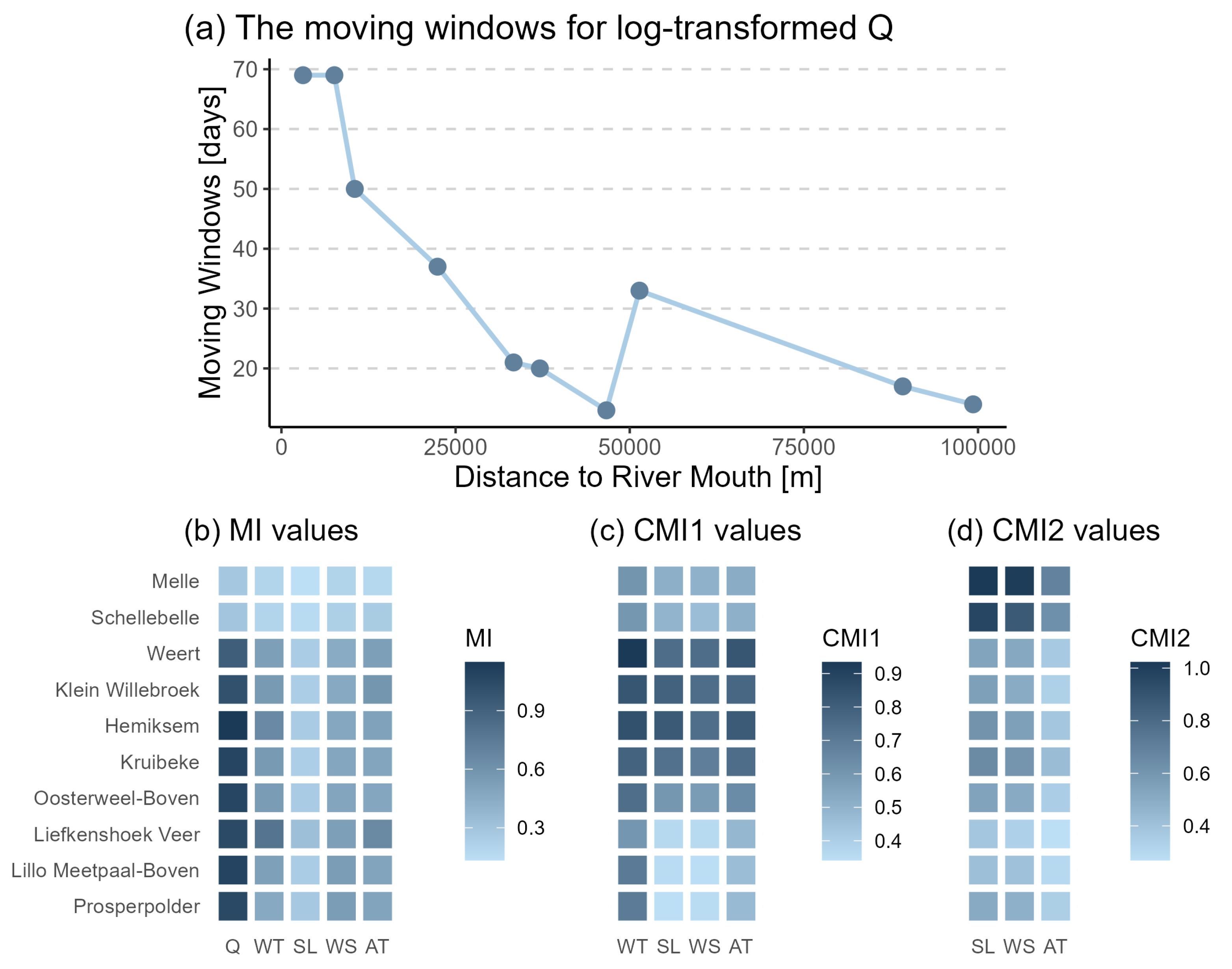
The initial DFs included the natural log-transformed X-day forward moving averaged Q, WT, AT, SL, and WS. First, the best moving average window (1 to 100 days) for natural log-transformed Q was determined based on the highest MI value between it and the salinity for each station, as shown in subplot (a) of Figure 2. Generally, the optimal moving average day decreases from downstream to upstream. Near the outlet area, where the Q and S vary largely, the moving windows are around 70 days. A rapid decline is apparent in the middle part from 70 to 30 days, where the tidal effect becomes weaker. In the upstream areas, where salinity concentration is lower than 0.5 psu all year round, it remains below 20 days.
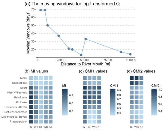
Figure 2.
The top panel indicates the optimal moving averaged days for log-transformed Q. The bottom panel shows MI, CMI1, and CMI2 values between the observed salinity and DFs (Q, WT, SL, WS, and AT) for the ten stations.
From top to bottom, Figure 2 shows MI values in subplot (b), CMI1 values in subplot (c), and CMI2 values in subplot (d) between the observed daily salinity and these DFs from downstream to upstream. The selection of DFs was determined based on the highest MI, CMI1, and CMI2 values. As the MI values of processed Q are obviously greater than the other four factors in subplot (b), Q was chosen as the dominant DF. The MI values for the other DFs are about half those for Q, but bigger than 0, which indicates that the salinity dispersion is also related to WT, SL, WS, and AT, although not as strongly.
The CMI1 values for the other four DFs conditioned on Q are shown in subplot (c). WT was selected as the second DF because of its relatively higher CMI values. Compared with AT, higher CMI1 values of WT can more directly affect the salinity diffusion. The CMI2 values for SL, WS, and AT conditioned on Q and WT are shown in subplot (d), it can be seen that all CMI2 values are close and small, which means that the mutual information between salinity and these three factors is similar. Because SL is slightly higher, it was chosen as the third DF. Unlike the decrease in MI values when moving inland, there is no obvious trend at the spatial scale for CMI1 and CMI2; hence, the X-day moving averaged natural log-transformed Q, WT, and SL were considered as the final input variables for modeling in this study.
4.2. Results of Models
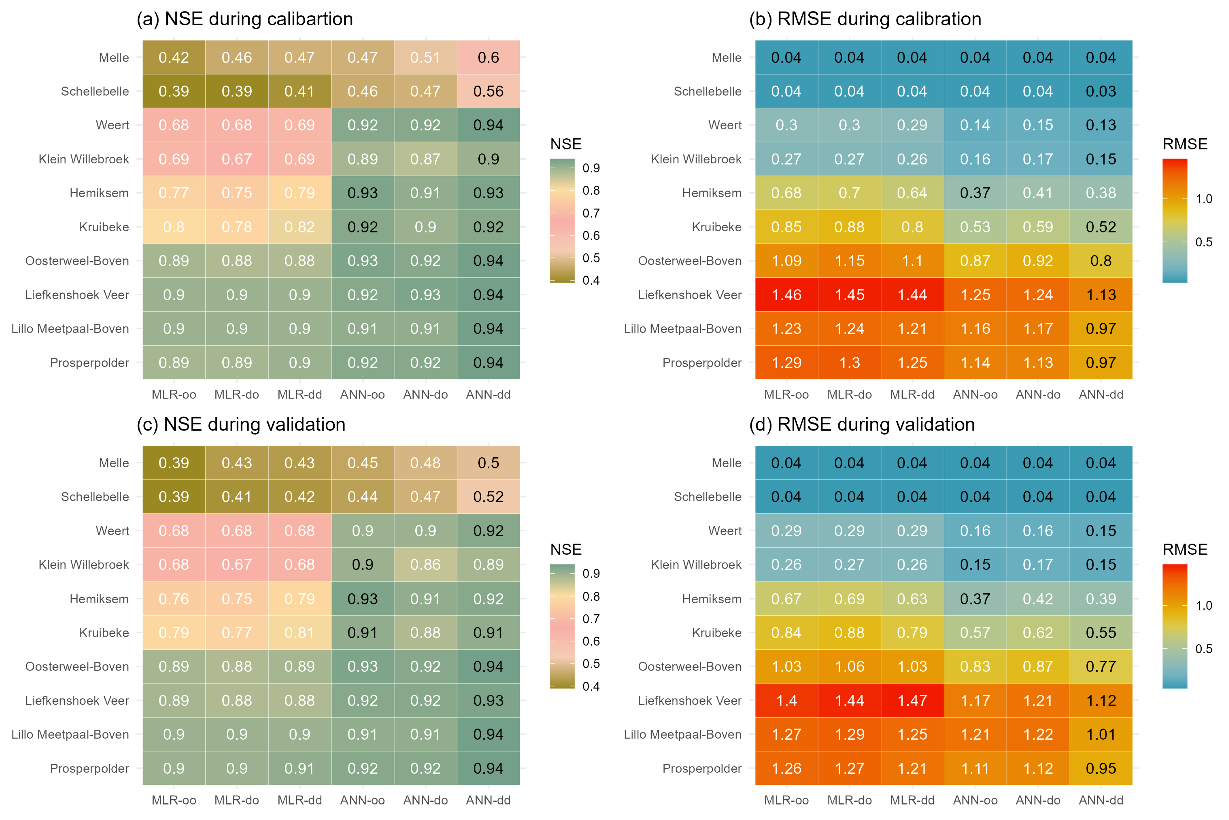
This study considers six DD models (see Figure 3). Each model differs from the other regarding the used technique (MLR or ANN) and DWT ensemble framework (SH or WH). Figure 3 presents the performance of the six models from upstream to downstream during the calibration and validation periods. The evaluation metrics of NSE and RMSE are calculated to assess the simulations spanning from the outlet to upstream.
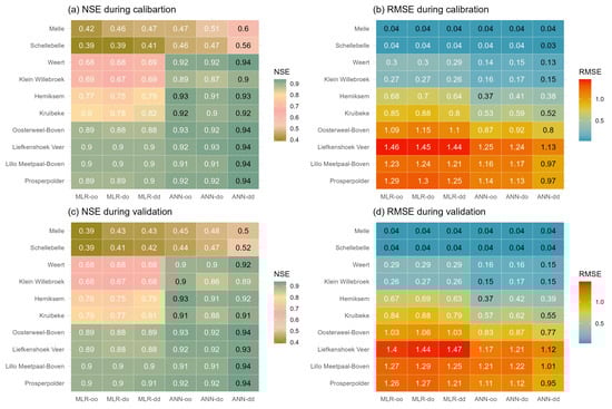
Figure 3.
Performance statistics (NSE and RMSE) for salinity simulations for the ten stations using six DD models during calibration and validation periods. The maximum NSE and Minimum RMSE values per station are highlighted in black.
In general, the simulation results from ANN models are much more accurate than MLR in both calibration and validation periods, with higher NSE and lower RMSE. As mentioned above, there are two main frameworks for coupling DWT in MLR and ANN models. With the SH framework, the performance of the models ‘MLR-do’ and ‘ANN-do’, which utilized the original salinity time series and decomposed DFs, does not exhibit any notable improvement in comparison to the ‘MLR-oo’ and ‘ANN-oo’ models. This indicates that applying the DWT solely to the DFs does not manifest as conspicuously as anticipated in this study. When juxtaposing ‘MLR-oo’ and ‘MLR-dd’ with ‘ANN-oo’ and ‘ANN-dd’, it becomes obvious that the outcomes achieved when implementing the WH framework surpass compared those for the models that use the SH framework. The ‘ANN-dd’ model performs best during the calibration period, with an NSE over 0.56 and RMSE lower than 1.13. A slight reduction in performance is observed in the validation accuracy, with NSE over 0.5 and RMSE lower than 1.12, though it remains within an acceptable and plausible range. Similarly, the simulation results of MLR simulation using DWT are better than ‘MLR-oo’ and ‘MLR-do’, although the improvements are not as obvious as for ANN.
As presented in Figure 3, the NSE values decrease from downstream to upstream for the MLR models, which decrease from 0.89 to 0.39 during the calibration period, and this trend remains for the validation dataset from the ’MLR-oo’ model. In subplots (b) and (d) for RMSE, an obvious spatial decreasing trend from downstream to upstream is observed, which is mainly due to the decreasing average salinity concentration along the river channel. Noticeably, a steep increase in RMSE is shown at the station ’Liefkenshoek Veer’, with a high RMSE value of 1.46 (1.4) during the calibration (validation) period. This is caused by excessive missing data leading to multiple discontinuities in the time series, making the sample size about half or less that of the other stations in Table 1.
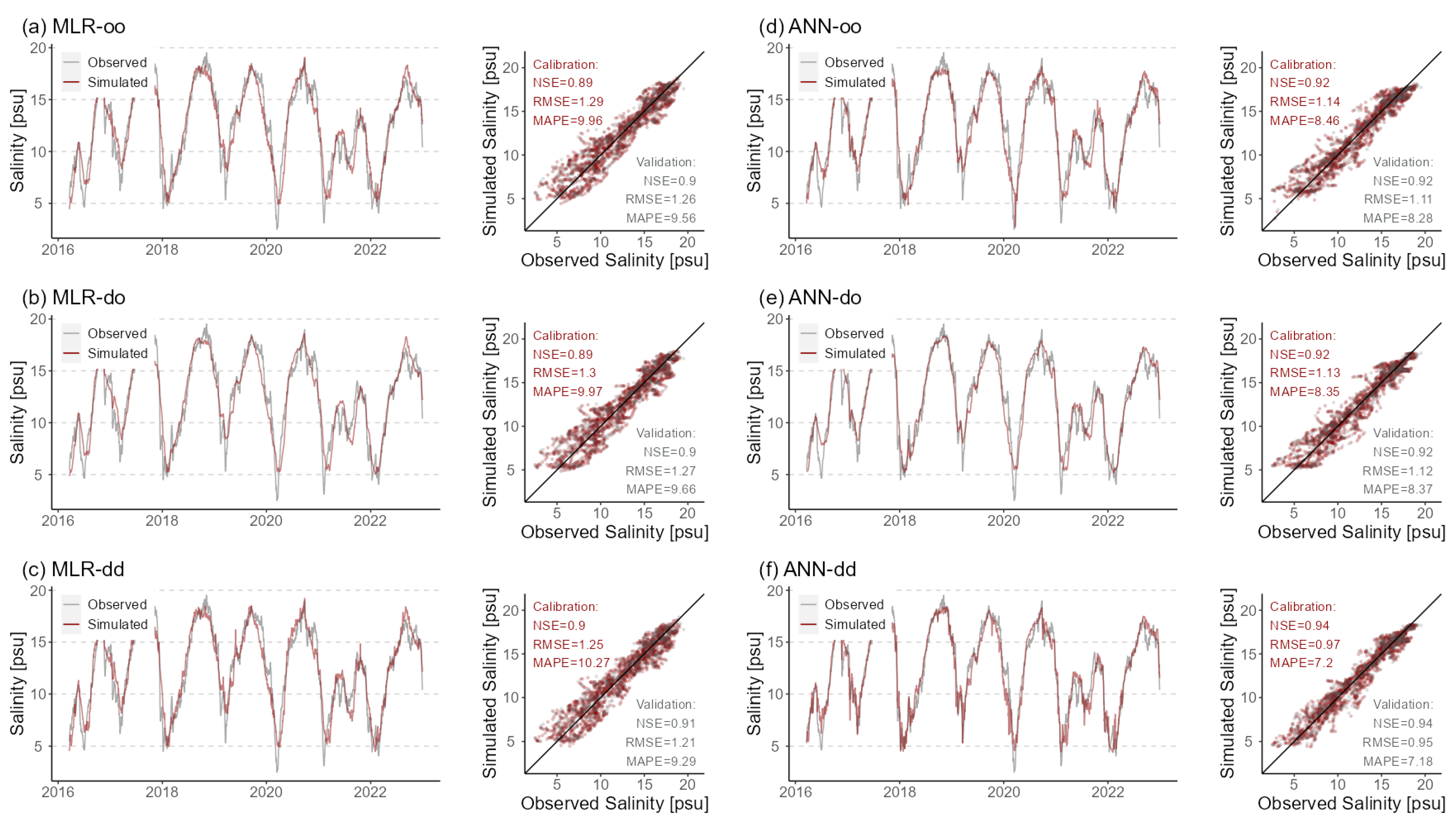
Figure 4 provides the observed and simulated salinity time series plots with six models at station ‘Prosperpolder’, which is only 3100 m away from the river mouth. Salinity concentrations at this station are very high, with peaks reaching 19.5 psu. Moreover, the correlations between salinity and the DFs are robust, which can be seen from the high MI and CMI values in Figure 2. Consequently, all DD models perform well at this station, showing high NSE and low RMSE in Figure 3. The time series plots in Figure 4 (the left panel in each subplot) reveal that these models exhibit a commendable and stable capacity to capture salinity variations, particularly the timing of rising and falling salinity. From the scatter plots in the right panel of each subplot, part of the data points from MLR models (in subplots (a), (b), and (c)) are significantly below the identity line, exhibiting a trend of underestimating the high values. The ANN models perform better in both the simulation and verification periods, where the problem of peak underestimation is significantly improved. With combined DWT, the overall scatters from ‘ANN-dd’ are much more densely distributed around the identity line, indicating better performance compared with ‘ANN-oo’, where the NSE increases from 0.92 to 0.94, RMSE decreases from 1.11 to 0.95, and MAPE decreases from 8.28 to 7.18 during the validation period.
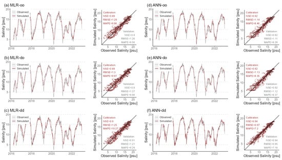
Figure 4.
Simulated and observed daily salinity time series at station ‘Prosperpolder’ using six models during calibration and validation periods. The right panel shows time series plots. The left panel shows scatter plots, where NSE, RMSE, and MAPE are calculated for calibration (in red) and validation periods (in grey).
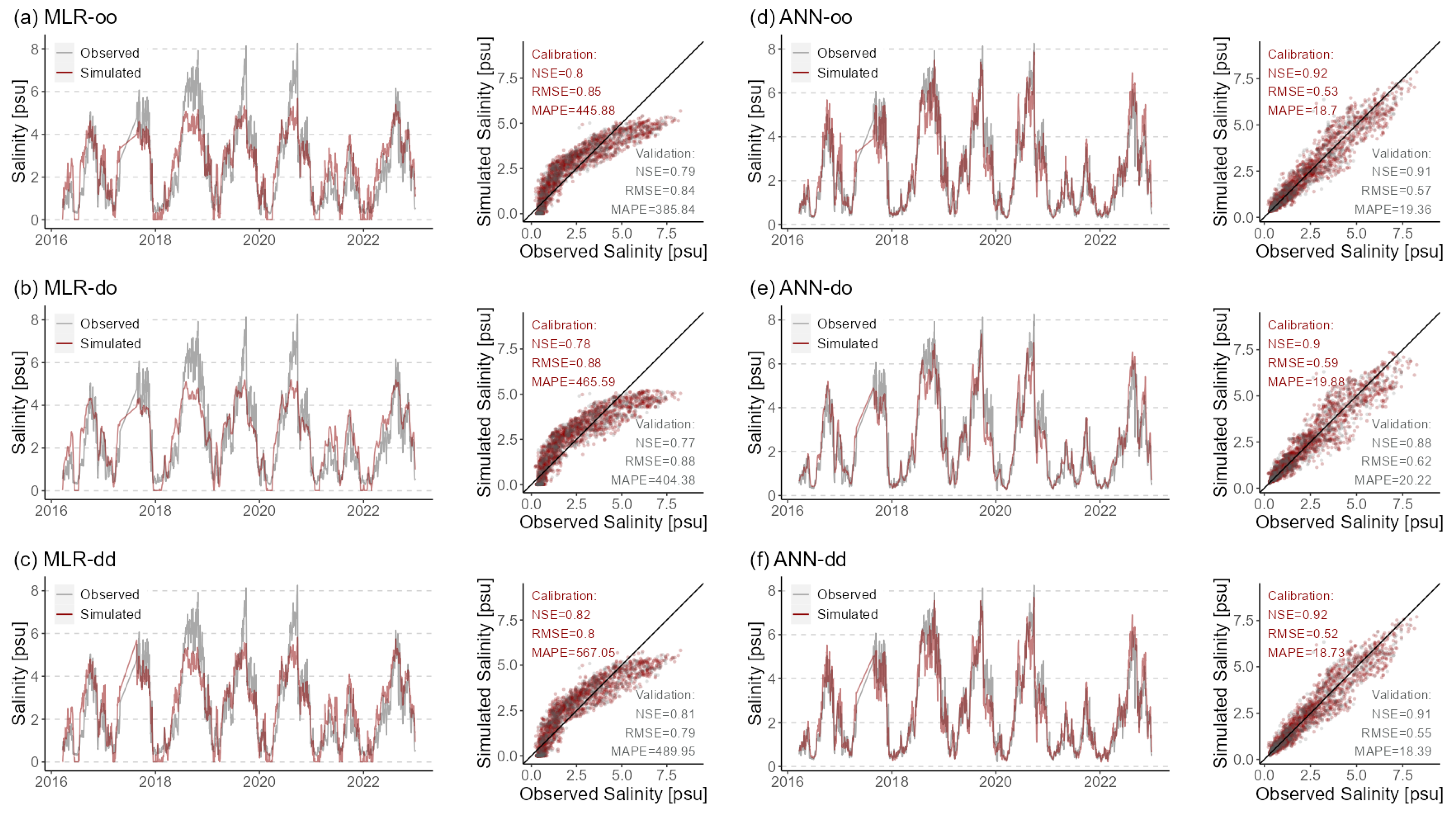
The simulations from station ‘Kruibeke’ are shown in Figure 5, which is 33,330 m away from the river mouth. Corresponding to Figure 3, the MLR models perform much worse than the ANN models in the middle reaches. The high salinity values are greatly underestimated, especially the three extreme values at around 8 psu shown in Figure 5, which are underestimated by about one-third. However, most low and medium values are overestimated except for a few extremely low salinity values. Considering the non-negativity of the salinity concentration, all negative simulations were set to 0. Although this high-value underestimation still exists in the ANN models, it is greatly improved, and the low-value simulations are also much better than for the MLR models.
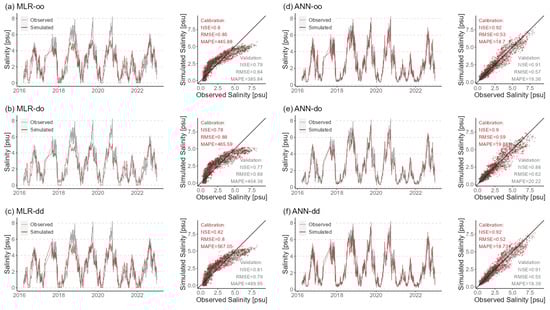
Figure 5.
Simulated and observed daily salinity time series at station ‘Kruibeke’ using six models during calibration and validation periods. Other information is the same as in Figure 4.
In the area downwards from station ‘Weert’, the simulation results of the ANN models far exceed the MLR performance of NSE > 0.75 [49]. All NSE values are greater than 0.85 in both the simulation and validation periods. Farther upstream, the effect of seawater intrusion diminishes while the impact of freshwater influx into the sea intensifies, resulting in a weakened correlation between these DFs and salinity. This amalgamation of factors contributes to the subpar simulation outcomes of the DD model at the upstream stations ‘Melle’ and ‘Schellebelle’, with all NSE values below 0.6, which is also consistent with the low MI values in Figure 2. Note the consistently low salinity levels upstream, which vary between 0.3 and 0.6 psu throughout the year. With the standard water supply limit being typically set at 0.5 psu and the limited influence on the nearby aquatic ecosystem and water abstractions, there is no requirement for high precision at these two stations.
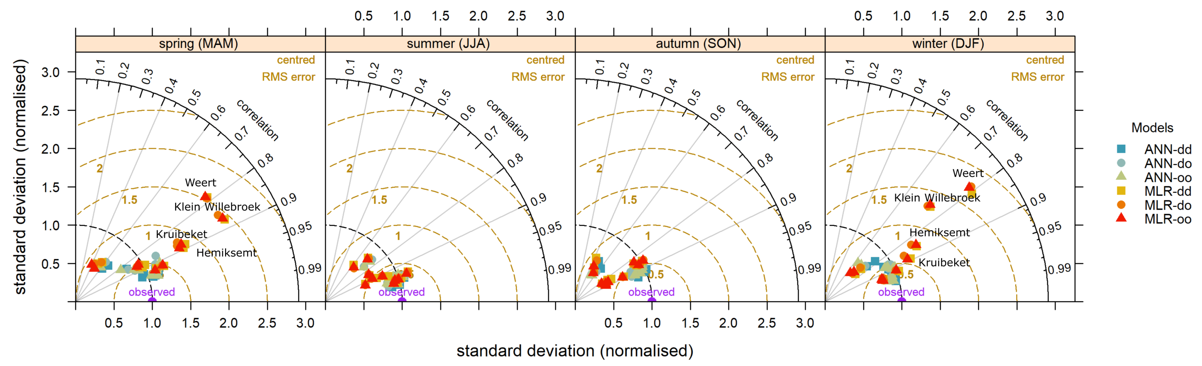
Analyzing seasonal patterns aids in ecosystem management and conservation efforts. Figure 6 shows the Taylor diagram of the six models over the four seasons of the validation period. The seasonal results from the ANN models are closer to the observed data than those from the MLR models, among which the ANN-dd model has the best performance with relatively low centered-RMSE. In addition, most of the points are located within the black dashed arc (normalized standard deviation = 1), indicating that their variations are smaller than observed. It is noticeable that the pattern of variations at these midstream stations (stations Kruibeket, Hemiksemt, Klein Willebroek, and Weert) have larger amplitude compared with the patterns observed during spring and winter. The performance of MLR models reveals notable success during the summer and autumn, while simulation capabilities are largely limited at most midstream stations during the spring and winter. The scatters representing the ANN models are more concentrated, and perform better all year round.
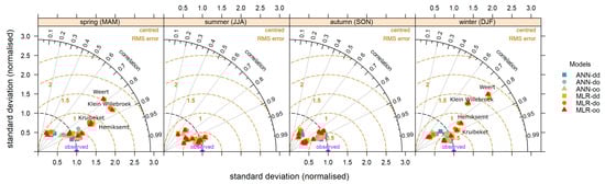
Figure 6.
Taylor diagram of seasonal salinity simulation for the ten stations using six models during the validation period.
4.3. Percentile Analysis
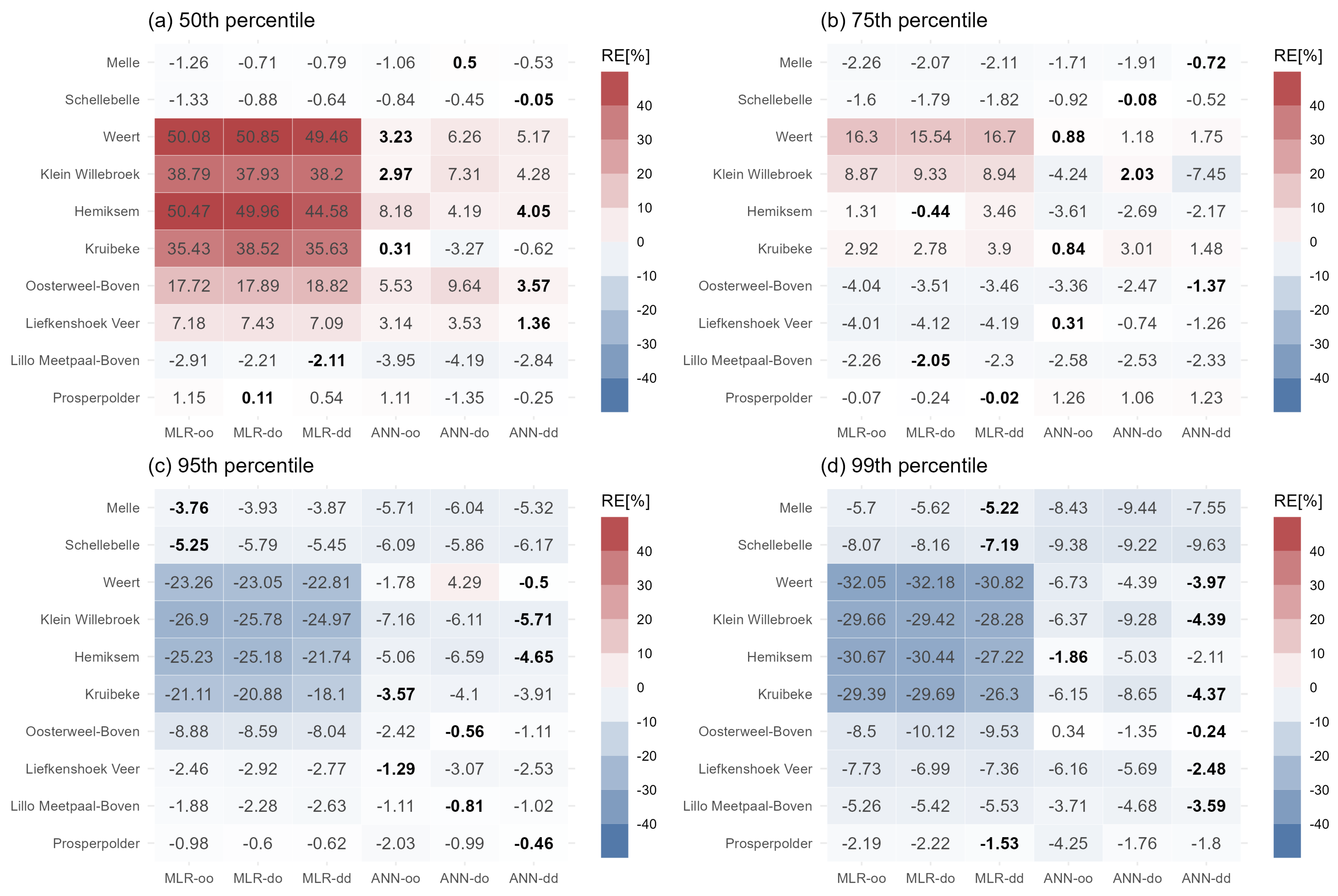
To investigate the simulations of high salinity along the studied river, the RE between observations and simulations during the validation period at different percentiles are compared in Figure 7. In evaluating simulations of the 50th (median), 75th (upper quartile), 95th, and 99th (extremes) percentiles of salinity by the six models, almost all models consistently overestimated the 50th percentile salinity. In contrast, simulations of the 95th and 99th percentile salinity were significantly underestimated. It is noticeable that the simulation of the 75th percentile salinity exhibited slight biases, indicating higher accuracy.
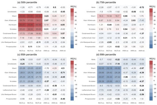
Figure 7.
RE between simulated and observed salinity at the 50th, 75th, 95th, and 99th percentiles from the six models during the validation period. The lowest RE values among the six models per station are shown in bold.
Because of the low average salinity and small variations for the two upstream stations ‘Melle’ and ‘Schellebelle’, these two sites were not included in the percentile comparison. In the 50th percentile analysis from subplot (a) of Figure 7, the RE values by the MLR models increase from 1.15% to 50.47% from downstream to upstream for the MLR-oo model. There is no obvious spatial feature for the ANN-dd model, with the RE varying between −0.25% and 5.17%. From the percentile heatmaps at the 95th percentile in subplot (c) and 99th percentile in subplot (d), underestimation becomes more pronounced when moving downwards along the river. Surprisingly, the biggest overestimation with RE of 50.05% at the 50th percentile is more severe than the biggest underestimation with RE of −32.05% for extremely high 99th percentile values.
The best model for each station is highlighted in Figure 7 in bold. The ANN models perform better in different percentile analyses than the MLR ones. As the percentile increases, the number of stations with the ANN-oo model as the optimal model continues to decrease from 4 to 1, while the number for ANN-dd models reaches the largest at the 99th percentile. The simulations for extremely high values improve as the model becomes more complex, which can be mutually confirmed from the previous time series and scatter plots in Figure 4 and Figure 5.
4.4. Sensitivity Analysis
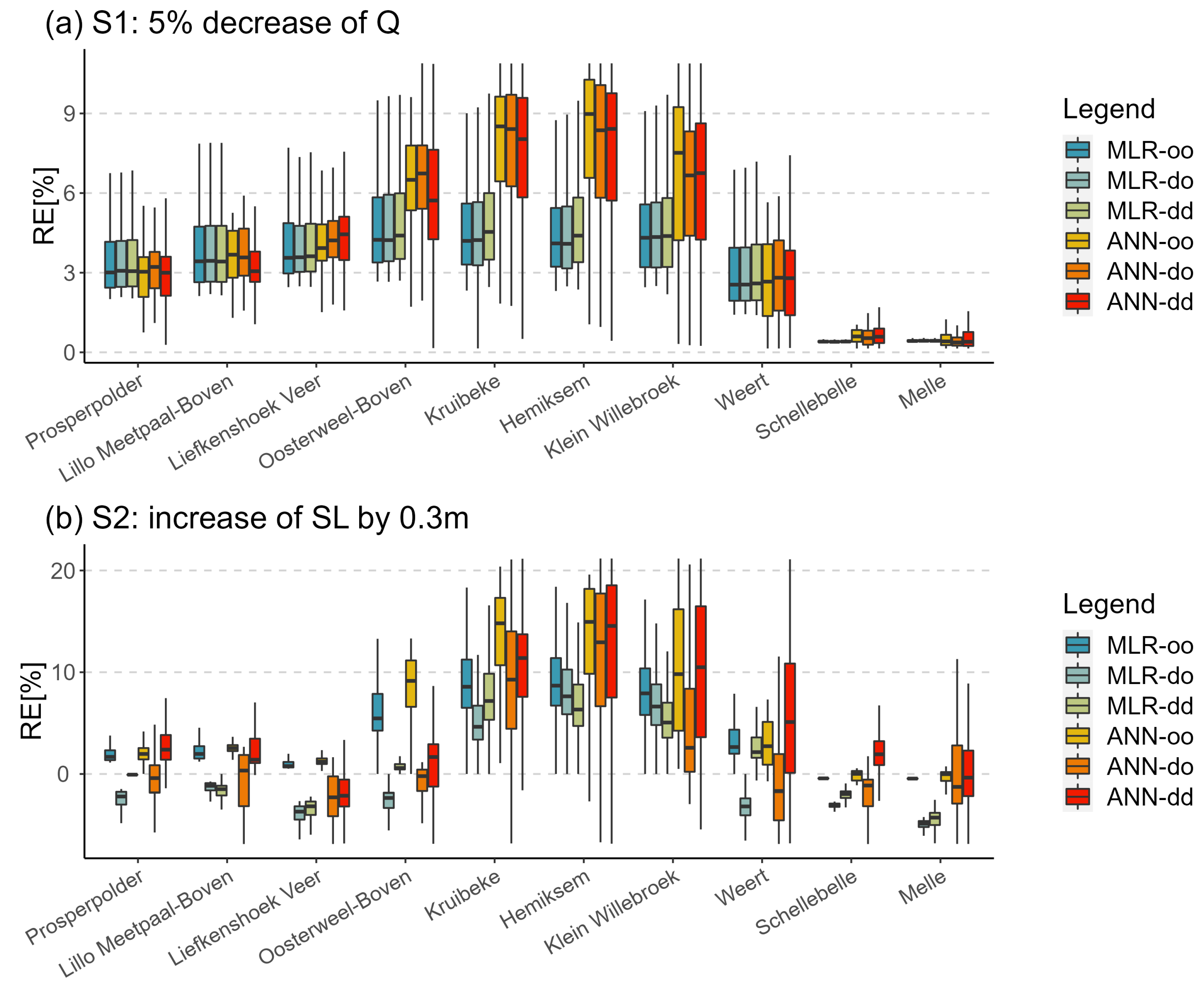
The sensitivity of DD models is evaluated by perturbing the corresponding DFs. Two scenarios, S1 (5% decrease of Q) and S2 (increase of WL by 0.3 m), were included to test how the salinity changes when disturbing different DFs. The RE values between historical and perturbed scenarios for the whole study period are calculated in Figure 8.
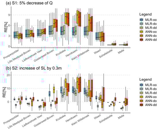
Figure 8.
RE between the perturbed scenarios and original simulations from the six models during the whole study period.
In subplot (a) of Figure 8, the RE values are above 0 in scenario S1, indicating that the salinity increases as Q decreases. The salinity variations show a trend of first increasing and then decreasing from downstream to upstream, which is especially obvious in the ANN models. For most of the stations, the modeled salinity is expected to increase between 3% and 6% for MLR models and the change range is between 3% and 9% for ANN models, with the main difference concentrated in the middle reaches of the river. In the previous model evaluation shown in Figure 3, the ANN models performed significantly better in the middle reaches which is the main reason for this difference in the sensitivity analysis.
Subplot (b) shows the salinity response to SL perturbation of 0.3 m. When SL rises, salinity intrusion becomes relatively intensified. The overall RE values corresponding to most simulations are greater than 0. The spatial variations in RE also show a trend of first increasing and then decreasing in scenario S2. Except for the two most upstream stations, the RE values from the ‘MLR-oo’ model are all greater than 0, fluctuating between 0 and 10%; however, there are negative RE values in nearly half of the simulation results from the ‘MLR-do’ and ‘MLR-dd’ models. This means that application of the DWT increases the uncertainty of the MLR models, making them unsuitable for salinity prediction under changing climate conditions. Except for a small number of low salinity values corresponding to RE less than 0, the simulated RE values for mean salinity events from ‘ANN-oo’ and ‘ANN-dd’ are both greater than 0, ranging from 0 to 20%, while the performance of ‘ANN-do’ is relatively poor.
5. Discussions
The imperative to ascertain salinity variations has been a longstanding concern, prompting contemporary investigations to employ diverse methodologies in temporally distributed salinity estimations at uncharted points [7,50]. This study utilizes and compares traditional statistical MLR and machine learning ANN methods to model daily salinity along the Scheldt Estuary in Belgium. To improve the models, the DWT is combined in two different frameworks, namely, SH and WH. In total, six models were constructed.
Optimal DFs serve as the foundation for guiding execution and advancing towards a dependable and accurate model output [8]. The forward moving averaged natural log-transformed Q is highly related to the salinity concentration, with moving windows ranging from 70 to 20 days along the Scheldt Estuary in Figure 2. In [51], it was pointed out that daily salinity concentrations are highly related to 30-day to 60-day averaged Q with least-squares regression near the Conowingo Hydroelectric Project at the mouth of the Susquehanna River, with the conclusions for the range of moving windows being almost consistent. Other studies have found that Q is the best salinity predictor for long-term salinity simulation [12,31]. Due to the certain correlation between WT and salinity, high-salinity events are relatively common during periods of high temperature and drought [3]. Studies indicate that the mixing of salinity can be related to the wind by altering salinity stratification [13,52], which is confirmed by the MI of WS being greater than 0. In addition, higher MI values can be observed in Figure 2 for all the DFs near the river mouth compared with the upstream area, which is consistent with the spatial distribution pattern of salinity concentration [10]. The DFs for salinity vary across different basins due to the distinct hydrological and geographical characteristics in previous studies [1,10,13]. In the case of the Scheldt Estuary, DFs of Q, WT, and SL were determined by the highest MI, CMI1, and CMI2 values.
Based on different calculation principles, this study involves the following six models with different simulation accuracy and construction difficulty: ‘MLR-oo’, ‘MLR-do’, ‘MLR-dd’, ‘ANN-oo’, ‘ANN-do’, and ‘ANN-dd’. Among these, the ‘MLR-oo’ model stands out as the most straightforward to construct. As a conventional DD model, MLR models boast simple construction, ease of use, and acceptable simulation accuracy in many cases [12,24]. Despite ‘MLR-oo’ exhibiting notable deviation from the observations, it is imperative to underscore that the majority results evince a robust NSE above 0.68 at most stations in the estuary, which meets the ‘satisfying’ standard of NSE > 0.36 [49]. The ‘ANN-oo’ model is a basic machine learning model with NSE above 0.88 and RMSE less than 1.64, a considerable improvement compared to the MLR models. This finding further underscores the intrinsic capacity of the ANN methodology to effectively capture the intricate nonlinear relationships between the independent and dependent variables [39].
From the heatmap of NSE and RMSE in Figure 3, the MLR models perform almost as well as the ANN models at downstream stations (stations Prosperpolder, Lillo Meetpaal, Liefkenshoek, and Oosterweel-Boven); however, their simulation accuracy is largely limited in the middle reaches (stations Kruibekes, Hemiksem, Klein Willebroek, and Weert). Specifically, comparing the results at the downstream Prosperpolder station in Figure 4 and the midstream Kruibeke station in Figure 5, the ‘bending’ shape of the scattered point distribution in the later station suggests that the relationship between salinity and DFs applicable to the former station is not optimal in this location. Thus, further testing was conducted using the natural log-transformed salinity instead of the original time series to calibrate the parameters of the MLR models. This adjustment greatly improved the simulation accuracy over the midstream reaches (e.g., NSE increases from 0.8 to 0.87 at Kruibeke station during validation), while leading to deteriorated simulation accuracy over the downstream reaches (e.g., NSE drops from 0.9 to 0.8 at Prosperpolder station during validation). Because the areas affected by high salinity (downstream) deserve more attention, this change is not adopted here. For further enhancement of simulation accuracy, readers may contemplate the substitution of more state-of-art models in [20,53].
It is important to note that the relationship between DFs and salinity can be influenced by geographical factors [54] such as river topography, vegetation cover, and precipitation patterns, leading to uncertainties in salinity distributions. Different types of human activity [55,56] such as agriculture, industry, and transportation can also contribute to changes in the relations between salinity and DFs in rivers. In the Scheldt River Estuary, the lower reaches after passing through Antwerp have widening water surfaces with a complex network of natural waterways and artificial channels, as shown in Figure 1. In contrast, the midstream area belongs to relatively natural river nets. These significant differences between downstream and midstream partly contribute to different performances in the middle and downstream areas with the same fixed-form MLR models, implying that the fixed regression equation can hardly be applied to the entire Scheldt Estuary, even with different coefficients. In Figure 6, the main difference in MLR models compared with the ANN models occurs over the midstream stations with relatively high centered RMSE during spring and winter. This also corresponds to overestimated middle–low salinity simulations in Figure 5 and positive RE at the 50th percentile salinity in Figure 7. Therefore, if we only focus on high salinity, this problem can be avoided by extracting high values in advance and then analyzing them through MLR modeling.
A general consensus exists that the DWT can increase the correlation between input and output variables and improve DD models [27,29,44], which explains the superiority of ‘MLR-dd’ and ‘ANN-dd’ models in the calibration periods. From the statistical indexes, except for the two most upstream stations in Figure 3, in comparisons between ‘ANN-oo’ and ‘ANN-dd’ (NSE increases around 0 to 0.03, RMSE decreases around 0 to 0.07), the application of DWT has a more pronounced positive impact on enhancing the simulation accuracy of the ANN machine learning mythology (see the performance of ‘MLR-oo’ and ‘MLR-dd’: NSE increases around 0 to 0.02, while RMSE decreases around 0 to 0.05). Overall, the application of the DWT improves the accuracy slightly in these DD models, which is most likely because the dominant DF of Q has already undergone data preprocessing (forward moving average method and natural log transformation). This proves that appropriate data preprocessing can largely reduce data noise and simulation complexity, thereby improving the simulation accuracy of DD models.
Except for the overall salinity simulation, high salinity in estuaries is a critical factor that shapes the ecology, biodiversity, and overall functioning of these dynamic environments [57]. Due to its straightforward linear features, MLR models struggle to effectively balance overall simulation and accurate representation of extreme events, as found in previous analyses [1]. The negative RE at the 99th percentile in Figure 7 indicates that all mentioned DD models consistently underestimate the extreme values, a trend consistent with the findings of [26]. While considering the overall simulation effect, the simulation accuracy for the low proportion of high salinity is inevitably affected. This is one of the main reasons for previous studies choosing to divide the dry and wet seasons in advance [52,56]; however, this may lead to a discontinuity between the alternation of seasons. In addition, application of the DWT improves high-salinity simulations when comparing RE values from the MLR models (‘MLR-oo’ vs. ‘MLR-dd’) and ANN models (‘ANN-oo’ vs. ‘ANN-dd’). Although underestimation remains present, it is been alleviated to an extent. This study also reports that the ANN model coupled with DWT can help to reduce the typical overestimation of low salinity and underestimation of high salinity in comparison with the basic ANN model [1]. Hence, integration of the DWT is highly recommended for high-salinity simulations in the Scheldt Estuary.
Sensitivity analysis represents a robust methodology for evaluating model structure and determining the key parameters influencing model behavior [58]. In this study, we tested the DD models’ physical plausibility by decreasing Q (adding SL), where the salinity of each station increased to varying degrees due to the reduced dilution (strengthened seawater encroachment). Similar results can be found in the sensitivity analysis from [43]. Previous research has also demonstrated that discharge reduction can increase saline intrusion under future drought scenarios [13,59]. The predicted increment of salinity decreases from upstream to downstream, whereas the percentage variable of RE more clearly shows the relative impact of DFs disturbances along the river network. From the RE, which first increases and then decreases from downstream to upstream in Figure 8, it can be observed that the salinity in the midstream area is more sensitive to disturbances in both Q and SL. This longitudinal salinity pattern mentioned above has also been identified in certain 3D salinity modeling studies [60,61], which is due to the weaker vertical stratification under SL rise or decreased freshwater scenarios. The ANN (MLR) models exhibit heightened sensitivity, leading to notable fluctuations in RE of 0% to 10% (0% to 6%) under S1 and RE of −5% to 20% (−5% to 10%) under S2. Considering that the simulation accuracy of ANN models is higher, the predicted variation range is more reliable. Furthermore, the analysis reveals many negative RE values in predicted salinity by the ‘MLR-do’ and ‘ANN-do’ models with the SH framework under S2. This observed trend contradicts the anticipated salinity diffusion patterns under the defined scenario [62]. Consequently, it suggests that the SH framework may not be appropriate for practical implementation.
6. Conclusions
This paper presents a comparison of traditional statistical (MLR) and machine learning (ANN) algorithms to simulate daily overall and high salinity along the Scheldt River estuary. Meanwhile, two ensemble approaches incorporating the DWT are tested. We demonstrate each model’s applicability and advantages by comparing six different models.
Our comprehensive inter-model comparison of simulation outcomes across six distinct models reveals noteworthy insights. The accuracy of DD models is strongly related to the connection between the external DFs and the target salinity concentration. In terms of the tide-influenced Scheldt Estuary, Q is the main DF of salinity diffusion, followed by WT and then SL. The application of moving averages over different days and natural log transformation on Q can significantly improve the accuracy of DD models. ANN models score better than MLR models in both overall and high salinity simulations at all ten stations, with the ‘ANN-dd’ model outperforming the others. With variations in the geographical environment and human activities affecting different reaches, the universal applicability of fixed-form MLR models is notably inferior to that of ANN models. The Scheldt River Estuary displays a complex network of artificial channels and natural rivers in its lower reaches, transitioning into natural flows in the middle and lower reaches. One approach that can address this complexity is to employ various types of MLR models or to predefine the division between the dry and wet seasons. A commonality among MLR and ANN models lies in their tendency to underestimate high salinity values. Applying the DWT with the WH framework could help to reduce the underestimation of maximum values, while employing the SH framework can lead to high uncertainties in real practices. In the rising SL or declining Q scenarios, salinity intrusion intensifies more in the middle areas. This shows that the salinity in the middle estuary area is more worthy of attention under the background of climate change.
Our research provides a reference for determining the optimal model depending on the desired goal and simplicity in other similar study areas. In general, the relatively parsimonious ‘MLR-oo’ model consistently yields trustworthy results with the lowest time cost, while the existence of certain deficiencies in seasonal simulation and high-value simulation is acknowledged. The findings stemming from the ANN models rooted in the basic ANN methodology underscore the prowess of machine learning techniques in delivering superior performance. Lastly, as embodied by ‘ANN-dd’, the integration of the DWT with the WH framework represents an advanced iteration that achieves enhanced results for both overall and high salinity simulations.
Author Contributions
B.Z.: methodology, software, formal analysis, investigation, writing—original draft, visualization. T.W.: data curation, writing—review and editing. J.D.M.: data curation, writing—review and editing. P.W.: writing—review and editing, supervision. All authors have read and agreed to the published version of the manuscript.
Funding
Boli Zhu has been funded by the China Scholarship Council (Grant No.201906710112).
Data Availability Statement
All data used in this paper can be downloaded from the website (https://www.waterinfo.be/ accessed on 5 December 2023).
Conflicts of Interest
The authors declare no conflicts of interest.
Abbreviations
The following abbreviations are used in this manuscript:
| ANN | Artificial Neural Network |
| AT | Air Temperature above 1.5 m |
| BP | Backpropagation |
| CMI | Conditional Mutual Information |
| DD | Data-Driven |
| DFs | Driving Forces |
| DWT | Discrete Wavelet Transform |
| LM | Levenberg–Marquardt |
| MI | Mutual Information |
| ML | Machine Learning |
| MLP | Multilayer Perceptron |
| MLR | Multiple Linear Regression |
| Q | Discharge |
| SH | Signal-Hybrid |
| SL | Sea Level |
| WH | Within-Hybrid |
| WS | Wind Speed |
| WT | Water Temperature |
References
- Zhou, F.; Liu, B.; Duan, K. Coupling wavelet transform and artificial neural network for forecasting estuarine salinity. J. Hydrol. 2020, 588, 125127. [Google Scholar] [CrossRef]
- Li, H.; Wang, C.; Liang, C.; Zhao, Y.; Zhang, W.; Grégori, G.; Xiao, T. Diversity and distribution of tintinnid ciliates along salinity gradient in the Pearl River Estuary in southern China. Estuar. Coast. Shelf Sci. 2019, 226, 106268. [Google Scholar] [CrossRef]
- Hu, J.; Liu, B.; Peng, S. Forecasting salinity time series using RF and ELM approaches coupled with decomposition techniques. Stoch. Environ. Res. Risk Assess. 2019, 33, 1117–1135. [Google Scholar] [CrossRef]
- Hinkel, J.; Lincke, D.; Vafeidis, A.T.; Perrette, M.; Nicholls, R.J.; Tol, R.S.J.; Marzeion, B.; Fettweis, X.; Ionescu, C.; Levermann, A. Coastal flood damage and adaptation costs under 21st century sea-level rise. Proc. Natl. Acad. Sci. USA 2014, 111, 3292–3297. [Google Scholar] [CrossRef] [PubMed]
- Apiratikul, R.; Ponpan, W.; Chonwattana, S. Application of MIKE Hydro River and QGIS Programs to Simulate and Visualize Dissolved Oxygen Concentrations in Maeklong River, Samutsongkhram Province, Thailand; Assoc Computing Machinery: New York, NY, USA, 2019; pp. 139–143. [Google Scholar] [CrossRef]
- Lam, N.T. Real-Time Prediction of Salinity in the Mekong River Delta; Springer: Singapore, 2020; pp. 1461–1468. [Google Scholar] [CrossRef]
- He, W.; Zhang, J.; Yu, X.; Chen, S.; Luo, J. Effect of Runoff Variability and Sea Level on Saltwater Intrusion: A Case Study of Nandu River Estuary, China. Water Resour. Res. 2018, 54, 9919–9934. [Google Scholar] [CrossRef]
- Lu, P.; Lin, K.; Xu, C.Y.; Lan, T.; Liu, Z.; He, Y. An integrated framework of input determination for ensemble forecasts of monthly estuarine saltwater intrusion. J. Hydrol. 2021, 598, 126225. [Google Scholar] [CrossRef]
- May, R.; Dandy, G.; Maier, H. Review of Input Variable Selection Methods for Artificial Neural Networks. In Artificial Neural Networks-Methodological Advances and Biomedical Applications; IntechOpen: London, UK, 2011. [Google Scholar]
- He, Y.; Chen, S.; Huang, R.; Chen, X.; Cong, P. Impact of upstream runoff and tidal level on the chlorinity of an estuary in a river network: A case study of Modaomen estuary in the Pearl River Delta, China. J. Hydroinform. 2019, 21, 359–370. [Google Scholar] [CrossRef]
- Gong, W.; Lin, Z.; Zhang, H.; Lin, H. The response of salt intrusion to changes in river discharge, tidal range, and winds, based on wavelet analysis in the Modaomen estuary, China. Ocean. Coast. Manag. 2022, 219, 106060. [Google Scholar] [CrossRef]
- Zhang, Z.; Cui, B.; Hui, Z.; Fan, X.; Zhang, H. Discharge-salinity relationships in Modaomen waterway, Pearl River estuary. Procedia Environ. Sci. 2010, 2, 1235–1245. [Google Scholar] [CrossRef]
- Uncles, R.J.; Stephens, J.A. The Effects of Wind, Runoff and Tides on Salinity in a Strongly Tidal Sub-estuary. Estuaries Coasts 2011, 34, 758–774. [Google Scholar] [CrossRef]
- Onabule, O.A.; Mitchell, S.B.; Couceiro, F. The effects of freshwater flow and salinity on turbidity and dissolved oxygen in a shallow Macrotidal estuary: A case study of Portsmouth Harbour. Ocean Coast. Manag. 2020, 191, 105179. [Google Scholar] [CrossRef]
- Zhang, X.; Deng, J. Affecting Factors of Salinity Intrusion in Pearl River Estuary and Sustainable Utilization of Water Resources in Pearl River Delta. In Sustainability in Food and Water; Springer: Dordrecht, The Netherlands, 2010; pp. 11–17. [Google Scholar] [CrossRef]
- Meire, P.; Ysebaert, T.; Damme, S.V.; Bergh, E.V.D.; Maris, T.; Struyf, E. The Scheldt estuary: A description of a changing ecosystem. Hydrobiologia 2005, 540, 1–11. [Google Scholar] [CrossRef]
- Zounemat-Kermani, M.; Batelaan, O.; Fadaee, M.; Hinkelmann, R. Ensemble machine learning paradigms in hydrology: A review. J. Hydrol. 2021, 598, 126266. [Google Scholar] [CrossRef]
- Tian, R. Factors controlling saltwater intrusion across multi-time scales in estuaries, Chester River, Chesapeake Bay. Estuar. Coast. Shelf Sci. 2019, 223, 61–73. [Google Scholar] [CrossRef]
- Meyer, E.S.; Sheer, D.P.; Rush, P.V.; Vogel, R.M.; Billian, H.E. Need for Process Based Empirical Models for Water Quality Management: Salinity Management in the Delaware River Basin. J. Water Resour. Plan. Manag. 2020, 146, 5020018. [Google Scholar] [CrossRef]
- Granata, F.; Nunno, F.D.; Modoni, G. Hybrid Machine Learning Models for Soil Saturated Conductivity Prediction. Water 2022, 14, 1729. [Google Scholar] [CrossRef]
- Banerjee, P.; Singh, V.S.; Chatttopadhyay, K.; Chandra, P.C.; Singh, B. Artificial neural network model as a potential alternative for groundwater salinity forecasting. J. Hydrol. 2011, 398, 212–220. [Google Scholar] [CrossRef]
- Maheswaran, R.; Khosa, R. Comparative study of different wavelets for hydrologic forecasting. Comput. Geosci. 2012, 46, 284–295. [Google Scholar] [CrossRef]
- Nourani, V.; Komasi, M.; Mano, A. A Multivariate ANN-Wavelet Approach for Rainfall–Runoff Modeling. Water Resour. Manag. 2009, 23, 2877–2894. [Google Scholar] [CrossRef]
- Adamowski, J.; Chan, H.F.; Prasher, S.O.; Ozga-Zielinski, B.; Sliusarieva, A. Comparison of multiple linear and nonlinear regression, autoregressive integrated moving average, artificial neural network, and wavelet artificial neural network methods for urban water demand forecasting in Montreal, Canada. Water Resour. Res. 2012, 48, W01528. [Google Scholar] [CrossRef]
- Hinge, G.; Piplodiya, J.; Sharma, A.; Hamouda, M.A.; Mohamed, M.M. Evaluation of Hybrid Wavelet Models for Regional Drought Forecasting. Remote Sens. 2022, 14, 6381. [Google Scholar] [CrossRef]
- Syed, Z.; Mahmood, P.; Haider, S.; Ahmad, S.; Jadoon, K.Z.; Farooq, R.; Syed, S.; Ahmad, K. Short–long-term streamflow forecasting using a coupled wavelet transform–artificial neural network (WT–ANN) model at the Gilgit River Basin, Pakistan. J. Hydroinform. 2023, 25, 881–894. [Google Scholar] [CrossRef]
- Quilty, J.; Adamowski, J. Addressing the incorrect usage of wavelet-based hydrological and water resources forecasting models for real-world applications with best practices and a new forecasting framework. J. Hydrol. 2018, 563, 336–353. [Google Scholar] [CrossRef]
- Alizadeh, M.J.; Kavianpour, M.R. Development of wavelet-ANN models to predict water quality parameters in Hilo Bay, Pacific Ocean. Mar. Pollut. Bull. 2015, 98, 171–178. [Google Scholar] [CrossRef] [PubMed]
- Li, S.; Wang, P.; Goel, L. A Novel Wavelet-Based Ensemble Method for Short-Term Load Forecasting with Hybrid Neural Networks and Feature Selection. IEEE Trans. Power Syst. 2016, 31, 1788–1798. [Google Scholar] [CrossRef]
- Kim, N.H.; Kim, D.H.; Park, S.H. Prediction of the Turbidity Distribution Characteristics in a Semi-Enclosed Estuary Based on the Machine Learning. Water 2024, 16, 61. [Google Scholar] [CrossRef]
- Chao, Y.; Farrara, J.D.; Schumann, G.; Andreadis, K.M.; Moller, D. Sea surface salinity variability in response to the Congo river discharge. Cont. Shelf Res. 2015, 99, 35–45. [Google Scholar] [CrossRef]
- Laprise, R.; Dodson, J.J. Environmental variability as a factor controlling spatial patterns in distribution and species diversity of zooplankton in the St. Lawrence Estuary. Mar. Ecol.-Prog. Ser. 1994, 107, 67. [Google Scholar] [CrossRef]
- Winterwerp, J.C.; Wang, Z.B.; van Braeckel, A.; van Holland, G.; Kösters, F. Man-induced regime shifts in small estuaries-II: A comparison of rivers. Ocean. Dyn. 2013, 63, 1293–1306. [Google Scholar] [CrossRef]
- Meester, J.D.; Willems, P. Assessing the power of non-parametric data-driven approaches to analyse the impact of drought measures. Environ. Model. Softw. 2024, 172, 105923. [Google Scholar] [CrossRef]
- Wen, W.; Timmermans, J.; Chen, Q.; van Bodegom, P.M. Monitoring the combined effects of drought and salinity stress on crops using remote sensing. Hydrol. Earth Syst. Sci. Discuss. 2022, 2022, 1–15. [Google Scholar] [CrossRef]
- Lerczak, J.A.; Geyer, W.R.; Ralston, D.K. The Temporal Response of the Length of a Partially Stratified Estuary to Changes in River Flow and Tidal Amplitude. J. Phys. Oceanogr. 2009, 39, 915–933. [Google Scholar] [CrossRef] [PubMed]
- Lingling Ni, D.W.; Wu, J. Mutual information-based approach for vine copula selection for hydroligical dependence modeling. In Risk Analysis Based on Data and Crisis Response beyond Knowledge: Proceedings of the 7th International Conference on Risk Analysis and Crisis Response, Athens, Greece, 15–19 October 2019; CRC Press: Boca Raton, FL, USA, 2019. [Google Scholar]
- Sharma, S.; Siddique, R.; Reed, S.; Ahnert, P.; Mejia, A. Hydrological Model Diversity Enhances Streamflow Forecast Skill at Short-to Medium-Range Timescales. Water Resour. Res. 2019, 55, 1510–1530. [Google Scholar] [CrossRef]
- Chen, L.; Singh, V.P.; Guo, S.; Zhou, J.; Ye, L. Copula entropy coupled with artificial neural network for rainfall-runoff simulation. Stoch. Environ. Res. Risk Assess. 2014, 28, 1755–1767. [Google Scholar] [CrossRef]
- Quilty, J.; Adamowski, J.; Khalil, B.; Rathinasamy, M. Bootstrap rank-ordered conditional mutual information (broCMI): A nonlinear input variable selection method for water resources modeling. Water Resour. Res. 2016, 52, 2299–2326. [Google Scholar] [CrossRef]
- Khan, M.M.H.; Muhammad, N.S.; El-Shafie, A. Wavelet-ANN versus ANN-Based Model for Hydrometeorological Drought Forecasting. Water 2018, 10, 998. [Google Scholar] [CrossRef]
- Karul, C.; Soyupak, S.; Çilesiz, A.F.; Akbay, N.; Germen, E. Case studies on the use of neural networks in eutrophication modeling. Ecol. Model. 2000, 134, 145–152. [Google Scholar] [CrossRef]
- Rath, J.S.; Hutton, P.H.; Chen, L.; Roy, S.B. A hybrid empirical-Bayesian artificial neural network model of salinity in the San Francisco Bay-Delta estuary. Environ. Model. Softw. 2017, 93, 193–208. [Google Scholar] [CrossRef]
- Amjady, N.; Keynia, F. Short-term load forecasting of power systems by combination of wavelet transform and neuro-evolutionary algorithm. Energy 2009, 34, 46–57. [Google Scholar] [CrossRef]
- Belayneh, A.; Adamowski, J.; Khalil, B.; Ozga-Zielinski, B. Long-term SPI drought forecasting in the Awash River Basin in Ethiopia using wavelet neural network and wavelet support vector regression models. J. Hydrol. 2014, 508, 418–429. [Google Scholar] [CrossRef]
- Percival, D.B.; Walden, A.T. Wavelet Methods for Time Series Analysis; Cambridge University Press: Cambridge, UK, 2000; Volume 4. [Google Scholar]
- Shafaei, M.; Kisi, O. Lake Level Forecasting Using Wavelet-SVR, Wavelet-ANFIS and Wavelet-ARMA Conjunction Models. Water Resour. Manag. 2016, 30, 79–97. [Google Scholar] [CrossRef]
- Barzegar, R.; Fijani, E.; Moghaddam, A.A.; Tziritis, E. Forecasting of groundwater level fluctuations using ensemble hybrid multi-wavelet neural network-based models. Sci. Total Environ. 2017, 599–600, 20–31. [Google Scholar] [CrossRef]
- Motovilov, Y.G.; Gottschalk, L.; Engeland, K.; Rodhe, A. Validation of a distributed hydrological model against spatial observations. Agric. For. Meteorol. 1999, 98–99, 257–277. [Google Scholar] [CrossRef]
- Bertels, D.; Willems, P. Climate change impact on salinization of drinking water inlets along the Campine Canals, Belgium. J. Hydrol. Reg. Stud. 2022, 42, 101129. [Google Scholar] [CrossRef]
- Salinity and Salt Wedge Encroachment Study, RSP 3.20. Conowingo Hydroelectric Project. 2012. Available online: https://mde.maryland.gov/programs/water/WetlandsandWaterways/Documents/ExelonMD/FERC/Conowingo-FRSP-3.20.pdf (accessed on 20 January 2022).
- Lin, Z.; Zhang, H.; Lin, H.; Gong, W. Intraseasonal and interannual variabilities of saltwater intrusion during dry seasons and the associated driving forcings in a partially mixed estuary. Cont. Shelf Res. 2019, 174, 95–107. [Google Scholar] [CrossRef]
- Ni, J.; Liu, R.; Li, Y.; Tang, G.; Shi, P. An Improved Transfer Learning Model for Cyanobacterial Bloom Concentration Prediction. Water 2022, 14, 1300. [Google Scholar] [CrossRef]
- Gaiolini, M.; Colombani, N.; Mastrocicco, M.; Postacchini, M. Seawater intrusion assessment along the Volturno River (Italy) via numerical modeling and spectral analysis. J. Hydrol. 2023, 626, 130289. [Google Scholar] [CrossRef]
- Feng, X.; Chen, J. Impacts of environmental factors and freshwater discharges from multiple river outlets on estuarine salinity variation in rainy season: A case study of the Pearl River Estuary in China. J. Hydrol. 2023, 623, 129784. [Google Scholar] [CrossRef]
- Vargas, C.I.C.; Vaz, N.; Dias, J.M. An evaluation of climate change effects in estuarine salinity patterns: Application to Ria de Aveiro shallow water system. Estuar. Coast. Shelf Sci. 2017, 189, 33–45. [Google Scholar] [CrossRef]
- Feher, L.C.; Osland, M.J.; Swarzenski, C.M. Estuarine salinity extremes: Using the Coastal Salinity Index to quantify the role of droughts, floods, hurricanes, and freshwater flow alteration. Estuar. Coast. Shelf Sci. 2023, 291, 108445. [Google Scholar] [CrossRef]
- Holvoet, K.; van Griensven, A.; Seuntjens, P.; Vanrolleghem, P.A. Sensitivity analysis for hydrology and pesticide supply towards the river in SWAT. Phys. Chem. Earth 2005, 30, 518–526. [Google Scholar] [CrossRef]
- Costa, Y.; Martins, I.; de Carvalho, G.C.; Barros, F. Trends of sea-level rise effects on estuaries and estimates of future saline intrusion. Ocean Coast. Manag. 2023, 236, 106490. [Google Scholar] [CrossRef]
- Chen, W.B.; Liu, W.C.; Hsu, M.H. Modeling assessment of a saltwater intrusion and a transport time scale response to sea-level rise in a tidal estuary. Environ. Fluid Mech. 2015, 15, 491–514. [Google Scholar] [CrossRef]
- Chua, V.P.; Xu, M. Impacts of sea-level rise on estuarine circulation: An idealized estuary and San Francisco Bay. J. Mar. Syst. 2014, 139, 58–67. [Google Scholar] [CrossRef]
- Ross, A.C.; Najjar, R.G.; Li, M.; Mann, M.E.; Ford, S.E.; Katz, B. Sea-level rise and other influences on decadal-scale salinity variability in a coastal plain estuary. Estuar. Coast. Shelf Sci. 2015, 157, 79–92. [Google Scholar] [CrossRef]

Disclaimer/Publisher’s Note: The statements, opinions and data contained in all publications are solely those of the individual author(s) and contributor(s) and not of MDPI and/or the editor(s). MDPI and/or the editor(s) disclaim responsibility for any injury to people or property resulting from any ideas, methods, instructions or products referred to in the content. |
© 2024 by the authors. Licensee MDPI, Basel, Switzerland. This article is an open access article distributed under the terms and conditions of the Creative Commons Attribution (CC BY) license (https://creativecommons.org/licenses/by/4.0/).