Article

Surface and Subsurface Water Impacts of Forestry and Grassland Land Use in Paired Watersheds: Electrical Resistivity Tomography and Water Balance Analysis

by
Éricklis Edson Boito de Souza
1,
Franciele de Bastos
1,†,
Pedro Daniel da Cunha Kemerich
2,
Marieli Machado Zago
3,
Éderson Diniz Ebling
1,
Elias Frank de Araujo
4,
Antonio Celso Dantas Antonino
5 and
José Miguel Reichert
1,5,*
1
Soils Department, Universidade Federal de Santa Maria (UFSM), Santa Maria 97105-900, RS, Brazil
2
Geosciences Department, Universidade Federal de Santa Maria (UFSM), Santa Maria 97105-900, RS, Brazil
3
Geology Course, Universidade Federal do Pampa, Caçapava do Sul 96570-000, RS, Brazil
4
Research Department, CMPC Celulose Riograndense, Guaíba 92703-470, RS, Brazil
5
Nuclear Energy Department, Universidade Federal de Pernambuco (UFPE), Recife 50740-545, PE, Brazil
*
Author to whom correspondence should be addressed.
Current address: Institute of Silviculture, Department of Forest and Soil Sciences, University of Natural Resources and Life Sciences, Vienna, A-1190 Vienna, Austria.
Water 2024, 16(15), 2191; https://doi.org/10.3390/w16152191 (registering DOI)
Submission received: 10 June 2024 / Revised: 9 July 2024 / Accepted: 25 July 2024 / Published: 2 August 2024
(This article belongs to the Special Issue Soil Dynamics and Water Resource Management)

Abstract

:
Global forest plantations are expanding, causing land-use changes and impacting the water cycle. This study assesses whether eucalyptus plantations reduce groundwater levels compared to grasslands in paired subtropical watersheds. The hydrological dynamics of surface and subsurface water were compared in three small watersheds in southern Brazil, mainly occupied by Eucalyptus saligna (Es-W, 79.9 ha), Eucalyptus benthamii (Eb-W, 82.1 ha), and degraded anthropized natural grassland (G-W, 109.4 ha). Rainfall, flow, and piezometric levels were monitored. Runoff, evapotranspiration, and water balance in the soil profile were estimated, and the subsurface environment was characterized using electrical resistivity tomography. During higher accumulated rainfall, water surplus increased for all watersheds. In the wet period (accumulated rainfall of 1098.0 mm), evapotranspiration was higher for eucalyptus (624.3 mm for Eb-W and 512.5 mm for Es-W) than for the grassland watershed (299.5 mm), resulting in the highest runoff in G-W (649.6 mm). During the dry period (accumulated rainfall of 478.5 mm), water deficit and withdrawal were mainly observed in forested watersheds, decreasing groundwater. Combining water balance and electrical resistivity tomography estimations results in a better understanding of the hydrological dynamics in paired watersheds with different land uses. This information is useful for developing best-practice management strategies for sustainable water resource use and forest production.

1. Introduction

Global forest plantations are expected to double by 2050 in response to increasing demand for forest products [1], with changes in land use and management [2] and impacts on various components of the water cycle [3,4]. Even though forest plantations positively contribute to ecosystem services and the conservation of native forests [5], the impact of this expansion is controversial, mainly regarding the effects on local communities [6], the use of exotic species with invasive potential [7,8] that impact on biodiversity [9], and alteration in water availability [10,11].
Understanding water use by forest plantations and the impact of this dynamic on the landscape is crucial for sustainable forest management [12]. Currently, most of the studies focus on surface hydrology, investigating the role of forest plantations in rainfall interception by a canopy and contribution to water flow regulation [3,4,13,14], erosion, and sediment yield [15,16], the establishment of guidelines for forest management, such as tillage [17] and planting density [18], moisture and permeability in distinct soils [19], and water quality monitoring [20].
Groundwater behavior is complex and depends on interactions among physical, geochemical, and biological aspects [21]. The association of surface and subsurface hydrology under different land uses contributes to integrating hydrological processes more comprehensively. Geophysical techniques have been applied to diverse environments and conditions to evaluate subsurface hydrology [22,23,24,25,26], providing information about aquifer dynamics concerning seasonal variations and anthropic effects.
Electrical resistivity tomography (ERT) is a non-invasive tool for subsurface investigation. Electrical resistivity values are influenced by soil properties such as porosity, clay content, moisture, and pore water conductivity [27], which helps in imaging subsurface structures and hydrogeological processes [28]. In South America, ERT has been applied to different geological conditions [29,30], but the effect of changing land use from grasslands to commercial forests on groundwater has not been addressed.
Characterizing subsurface hydrology in forest plantations and integrating this information with water balance estimation allows for a better understanding of water dynamics. With climate change, increases in temperature and variations in precipitation patterns are occurring, potentially leading to longer drought periods [31]. Under drought conditions, trees can switch water uptake from superficial to deeper soil layers, which may affect groundwater [32]. Knowing the ecophysiological behavior of different species under environmental conditions is also important for forest management operations. Water use efficiency tends to vary for different eucalyptus species under the same environmental conditions [33]. A clear comprehension of this variability can help alleviate the impact of water scarcity by selecting more water-efficient species that decrease water use on the watershed scale.
Thus, studies evaluating groundwater resources in forest plantations are crucial for understanding the effects of silvicultural activities on hydrological variables. The study objective was to assess whether eucalyptus plantations reduce groundwater levels in paired subtropical watersheds compared to grasslands.

2. Materials and Methods

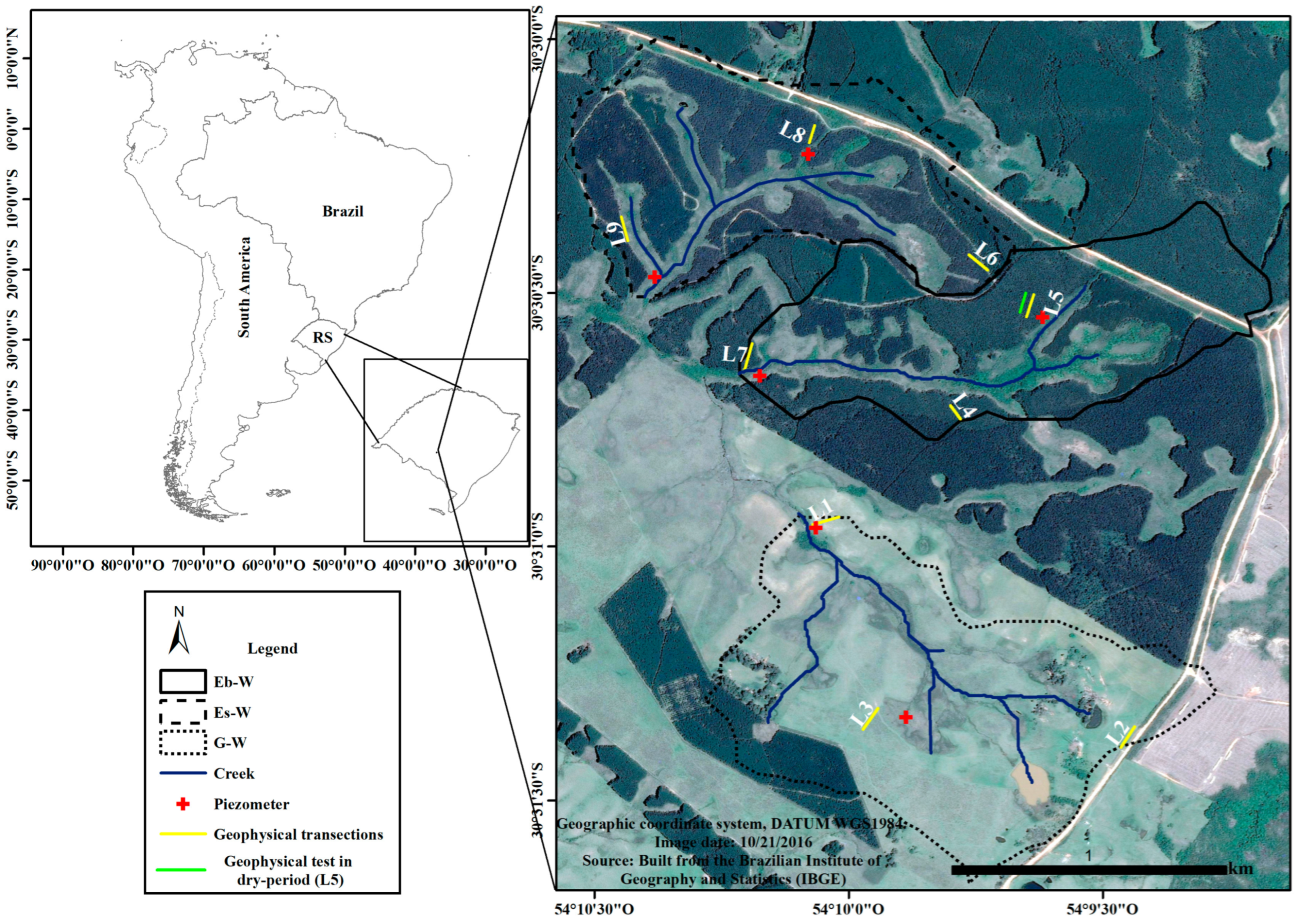
2.1. Study Watersheds

The study area is located in southern Brazil, at a latitude of 30°19′51″ S and a longitude of 54°19′32″ W. According to Köppen’s classification, the regional climate is Cfa, which corresponds to a subtropical climate. The mean elevation, annual temperature, and annual rainfall are 114 m, 18.6 °C, and 1356 mm, respectively [34,35].
The study area comprises three paired small rural watersheds (Figure 1). Two watersheds consist predominantly of eucalyptus plantations for cellulose production: one under cultivation with Eucalyptus saligna (Es-W) since 2006, which underwent a partial harvest of 30% in February 2014; and another watershed had a prior rotation of E. saligna clear-cut in 2014 and subsequent planting of E. benthamii (Eb-W) [36]. The third watershed is composed mainly of degraded natural and anthropized grassland (G-W) for extensive cattle production [4]. The paired watersheds approach assumes similar characteristics between watersheds to assess the effects of land use change on water resources. The Es-W, Eb-W, and G-W are second-order watersheds and were chosen because of their similar areas (0.83, 0.80, and 1.10 km²), altitudes (271, 258, and 284 m), and slopes (7.7, 6.2, and 3.9%), differing mostly in their land use.
Land use in Es-W is composed of clonal E. saligna plantations (61%) with a tree stocking of 1225 trees ha−1, native grassland and shrubs (30%), roads (6%), and rock outcrops (3%). In Eb-W, land use comprehends E. benthamii plantations (65%) with a tree stocking of 1225 trees ha−1, native grassland and shrubs (32%), and roads (3%), while in G-W, land use is based on degraded anthropized natural grasslands (71%), pasture (24%), grassland and shrubs (2.6%), an artificial dam (1.4%), and roads (1%). The eucalyptus plantations in Es-W were planted in 2006 (65%) and 2014 (35%), with a tree spacing of 3.0 × 3.3 m, resulting in a tree stocking of 1225 trees ha−1 and stand age of approximately 14 and 6 years. In Eb-W, the eucalyptus plantation was established in 2014, with a tree spacing of 3.0 × 2.2 m, a tree stocking of 1515 trees ha−1, and a stand age of approximately 6 years.
Local geology consists of orthogneisses, metadiorites from the Cambaí Complex stratigraphic unit, sandstones, and siltstones from the Rio Bonito Formation [4]. According to Soil Taxonomy [37] and the Brazilian Soil Classification System [38], the soils in the study area are classified as Udults (Argissolos Vermelhos), predominant on gentle interfluves, and higher landscape areas, Orthents (Neossolos Regolíticos) on steep slopes, and Aquults (Planossolos Háplicos) on lowlands [14]. The soils in all watersheds are considered physically fragile due to the predominant sandy texture and fast water infiltration, resulting in high susceptibility to surface erosion [14].

2.2. Hydrological Monitoring

Hydrological monitoring was conducted for each watershed from 1 January 2019 to 4 June 2020. Automatic tipping-bucket rain gauges (TB4 model from Campbell Scientific Instruments) were installed at each fluviometric station [14] and calibrated according to Reichert et al. [36]. Flow measurements were taken at automated streamflow purpose-built gauging stations, which include spillways equipped with water level sensors (Float-type water level sensor—Thalimedes, OTT Hydrometrie). Streamflow was calculated based on hydraulic equations considering the water depth in each spillway [36] and converted into millimeters based on the watershed area and time. Groundwater level data were collected from piezometers positioned in each watershed’s upper and lower sections, totaling two piezometers per watershed. Water levels were recorded hourly using dataloggers.

2.3. Water Balance

2.3.1. Water Balance at the Watershed Scale

The water balance was estimated using the mass conservation method [4], which calculates the water balance by comparing precipitation inputs and outputs such as evapotranspiration, runoff, and changes in soil water storage. Surface and subsurface drainage boundaries were assumed to coincide, with no subsurface exchange with adjacent areas. The temporal series considered for this study spanned from 1 January 2019 to 4 June 2020. However, to align water balance data with ERT results, 197 days were chosen. This period represents the difference between two geophysical surveys defined as wet (5 June 2019 to 19 November 2019) and dry (20 November 2019 to 4 June 2020) periods.
Reference evapotranspiration (ETo) was calculated using the FAO Penman–Monteith method [39], assuming grass as the reference crop. Climate data were obtained from a weather station owned by the Brazilian National Institute of Meteorology, located approximately 20 km from the study area. Due to the mature stage of the eucalyptus stands, leading to little change in leaf area and consequently in the rainfall interception by the plants, plant interception (INT) was estimated based on percentages reported by Ferreto et al. [3] for Es-W (26.8%), Eb-W (22.7%), and G-W (13.6%) during the period from October 2014 to September 2018. The available water capacity of the soil down to the root-system effective depth was 98.2 mm for Eb-W, 88.4 mm for Es-W, and 64.2 mm for G-W, previously defined by Ferreto et al. [3].
For water balance calculation on the watershed scale, rainfall was considered the only input into the system, while evapotranspiration, water intercepted by vegetation, soil water evaporation, plant transpiration, and runoff were the main outputs (Equation (1)).
Pyr − Qyr − ETayr − INTyr ± ΔSyr = 0,
where Pyr: total precipitation in the year i (mm), Qyr: runoff in the year i (mm), ETayr: soil evaporation and plant transpiration in the year i (mm), INTyr: water intercepted by vegetation in the year i (mm), and ΔSyr: variation of water storage in the watershed for the year i (mm).
By assuming ΔSyr = 0, the actual evapotranspiration (ETa) was calculated using Equation (2).
ETayr = Pyr − Qyr − INTyr = 0,
where ETayr: soil evaporation and plant transpiration in the year i (mm), Pyr: total precipitation in the year i (mm), Qyr: runoff in the year i (mm), and INTyr: water intercepted by vegetation in the year i (mm).

2.3.2. Water Balance in the Soil Profile

Water balance in the soil profile was determined using a sequential method adapted from Thornthwaite and Mather [40], covering the period from 01 January 2019 to 15 June 2020. Input parameters included total monthly precipitation (Pt), runoff (Q), reference evapotranspiration (ETo), and water intercepted by vegetation (INT).
As the main output parameters in this method, monthly evapotranspiration demand of vegetation not met due to water deficit (DEF), water surplus after satisfying evapotranspiration demand (EXC), replacement of water storage within the root zone (REP), soil water storage (S), and withdrawal of water that was previously stored in the soil to meet evapotranspiration demand (RET) were obtained.

2.4. Subsurface Characterization

Electrical resistivity tomography (ERT) was employed near piezometers of the study area to gather information on subsoil composition, particularly water content. Two geophysical monitoring campaigns were conducted: the first, called the wet period, on 19 November 2019, represents the rainy period, and the second, called the dry period, on 4 June 2020, represents a below-average rainfall period. ERT was performed using a Syscal Pro resistivity meter (IRIS Instruments®, Orléans, France) with 72 channels, following the method proposed by NBR 15.935/2011 [41]. Nine transects were scanned, each with a maximum length of 90 m, using a dipole–dipole arrangement with an electrode spacing of 5 m (Figure 1).
Data pre-processing was performed with Prosys II software (V3.14) from Iris Instruments® for data transfer, profile topography insertion, and raw data quality control. During the quality control process, negative resistivity values were removed from raw data, and the standard deviation of resistivity was controlled. Subsequently, Res2Dinv® software (V3.53) was used for data processing, which involved the inversion of apparent electrical resistivity values. The inversion process efficiently transforms the data into parameters that model subsurface structures. A technique for inverting resistivity data based on least squares and smoothness-constrained methods was employed [42,43]. This technique creates a 2D subsurface model from resistivity data obtained through electrical imaging surveys.
The interpretation of ERT sections considered electrical resistivity values of materials present in the study area, along with the porosity and permeability of sedimentary rocks (sandstones of the Rio Bonito Formation) and clayey layers. Electrical resistivity values were categorized into four zones based on the acquisition area and resistivity values:
1. Saturated zone: electrical resistivity ranges from 33 to 180 Ω·m (colors from deep blue to light blue). Low resistivity indicates the presence of subsurface water layers found within sedimentary rocks with high porosity and low permeability, enabling fluid percolation.
2. Intermediate zone I: electrical resistivity ranges from 180 to 1700 Ω·m (colors from light blue to moss green). This zone typically represents the contact area between the saturated zone and rocks with lower water content amid grains or areas with medium-grained sandstones. This zone may also relate to sandy-clay soils acting as a sealant for the strongly saturated zone.
3. Intermediate zone II: electrical resistivity ranges from 1700 to 5022 Ω·m (colors from moss green to orange). This zone comprises medium to fine unsaturated sandstones and serves as a transitional area with unsaturated igneous rocks at its base.
4. Unsaturated zone: electrical resistivity ranges from 5022 to 11605 Ω·m (colors varying between orange and purple). This zone is associated with unsaturated sandstones and/or rocks from the rock base, possibly granites.
To quantify each zone of the four zones, proportional ratios were applied to each line, delineating each section using AutoCAD® (Version 2020, Autodesk). This approach allowed the comparison of geophysical survey lines.

3. Results and Discussion

3.1. Surface Hydrology

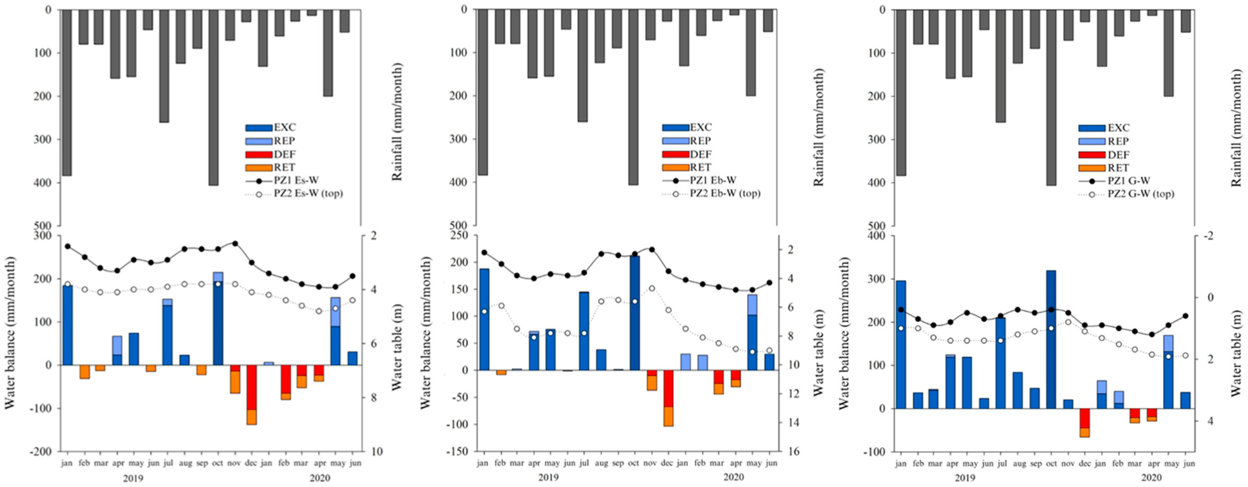
3.1.1. Water Balance at the Watershed Scale

The hydrological variables—rainfall, runoff, water intercepted by vegetation, soil evaporation, and evapotranspiration (Table 1)—varied between the dry and wet periods and among the watersheds. During the wet period, the accumulated rainfall in the paired watersheds was 1098.0 mm. Evapotranspiration was higher in the eucalyptus watersheds, resulting in 624.3 mm for Eb-W and 512.5 mm for Es-W. Evapotranspiration for the grassland watershed was almost half the observed for the eucalyptus watersheds (299.5 mm). Despite higher evapotranspiration, water intercepted by vegetation was higher for Es-W (356.1 mm) than for Eb-W (248.4 mm), while runoff was similar among the forest watersheds. As observed for evapotranspiration, water intercepted by vegetation for the grassland watershed (149.4 mm) was also almost half that observed in the eucalyptus watersheds, resulting in the highest runoff among the evaluated watersheds (649.6 mm).
During the dry period, the accumulated rainfall in the paired watersheds was 478.5 mm. The lower precipitation resulted in higher evapotranspiration in Eb-W (347.6 mm) compared to Es-W (257 mm), while water intercepted by vegetation was higher for Es-W (153.4 mm) compared to Eb-W (108.3 mm). For the grassland watershed, despite the lower water intercepted by vegetation (65.1 mm) compared to the eucalyptus watersheds, evapotranspiration (328.7 mm) exceeded that of Es-W. As observed during the wet period, runoff for the grassland was higher than for the eucalyptus watersheds (Table 1). The evapotranspiration for the grassland was slightly higher during the dry period (328.7 mm) than during the wet season (299.5 mm), which may be attributed to the occurrence of summer months in the southern hemisphere affecting seasonal plant behavior.
The greater evapotranspiration and interception observed for Eb-W and Es-W result from the higher evapotranspiration demands of tree species compared to grasslands. Similar results were observed in previous studies, where Es-W and G-W were compared in the initial rotation [14], resulting in a higher runoff for G-W. Even though grassland is the native vegetation for this environment, grazing activities result in soil compaction and a reduction in aboveground biomass, favoring the occurrence of erosion processes.
Variations in evapotranspiration and water intercepted by vegetation in Eb-W and Es-W result from stand traits. Despite the similar tree spacing among the forest watersheds (1225 and 1515 trees ha−1 for Es-W and Eb-W, respectively), Eb-W has approximately half of the stand age observed in 65% of the total area of Es-W, which may result in stand productivity differences [44]. However, intrinsic species characteristics may also contribute to differences in water use. Eucalyptus species have significant morphological differences, such as leaf inclination, shape, and stomatal index [45,46]. These factors impact species’ ecophysiology. Under the same site and climatic conditions, three different eucalyptus species used resources differently, resulting in tree transpiration rates of 1249, 928, and 733 mm y−1 for E. saligna, E. benthamii, and E. dunnii, respectively [33].

3.1.2. Water Balance in the Soil Profile

The sequential water balance, adapted from Thornthwaite and Mather [40], was calculated for each watershed (Figure 2). This approach encompasses measurements of the components’ excess water after satisfying evapotranspiration demand (EXC), replenishment of water storage within root zone (REP), evapotranspiration demand not satisfied because of water deficit (DEF), and soil profile water withdrawal by plants (RET).
Rainfall effect on water fluxes was observed for all watersheds (Figure 2). During months with higher accumulated rainfall, such as January, July, and October 2019, water surplus increased for all watersheds, with higher EXC for G-W, Es-W, and Eb-W, respectively. The highest water surplus was observed in the G-W watershed during the whole study period, with water deficit and water withdrawal occurring only during three months of lower rainfall in the current and previous months, in the summer and autumn of the southern hemisphere.
There was a significant base flow contribution to streams from groundwater during the wet season at the site G-W. This is corroborated by the observation that the water table remained shallow (<2 m) during this period, as indicated in Figure 3. The ERT results show zones of low resistivity along the profiles, indicating the presence of water and, consequently, the interaction between the water table and streams, contributing to base flow during the rainy months.
For the eucalyptus watersheds, excess water after satisfying the evapotranspiration demand was higher for Es-W compared to Eb-W. This behavior is confirmed by the greater frequency and more negative values of water deficit and water withdrawal for Eb-W than for Es-W. Increased evapotranspiration reduces subsurface water recharge, and plants use groundwater to develop [47]. This behavior is characterized as a drought-avoidance strategy and varies between species. Species that are more conservative in water use tend to invest more energy in fine root production than in leaf area [48]. Therefore, forest managers should consider climatological zoning and develop strategies based on regional water balance, considering interannual variation in rainfall, to plan sustainable practices related to forest water consumption and water inflow into the system [49].
The elevation differences of the piezometers corresponded to 54.8, 29.9, and 31.0 m, respectively, for Eb-W, Es-W, and G-C. By comparing these significant differences in upper-lower piezometer elevations (greater than 29 m) with the depths to the water table (less than 10 m during the studied period) in all three watersheds (Figure 2), we expect groundwater flow direction to move from the upper to the lower portion of the watershed.

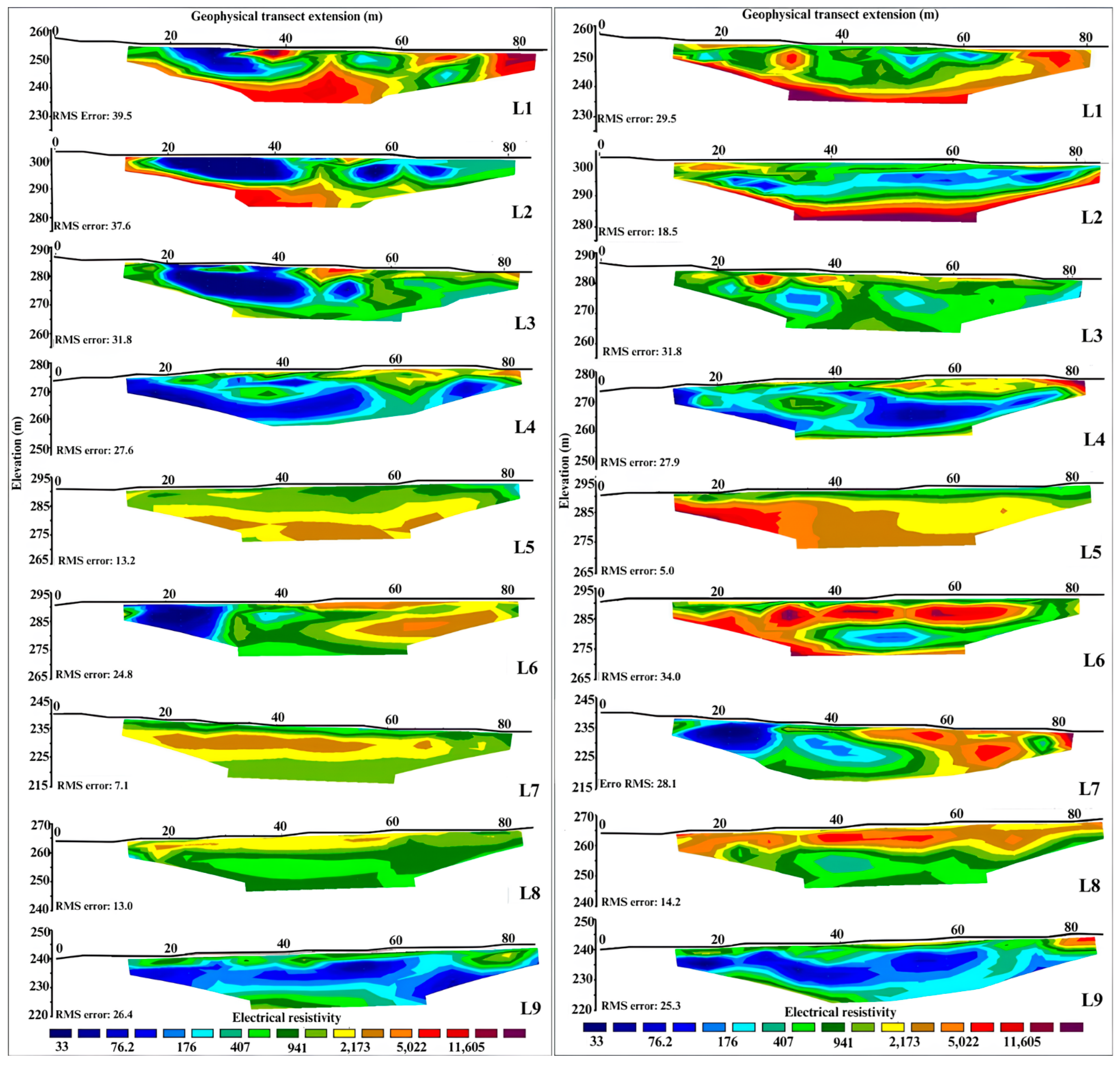
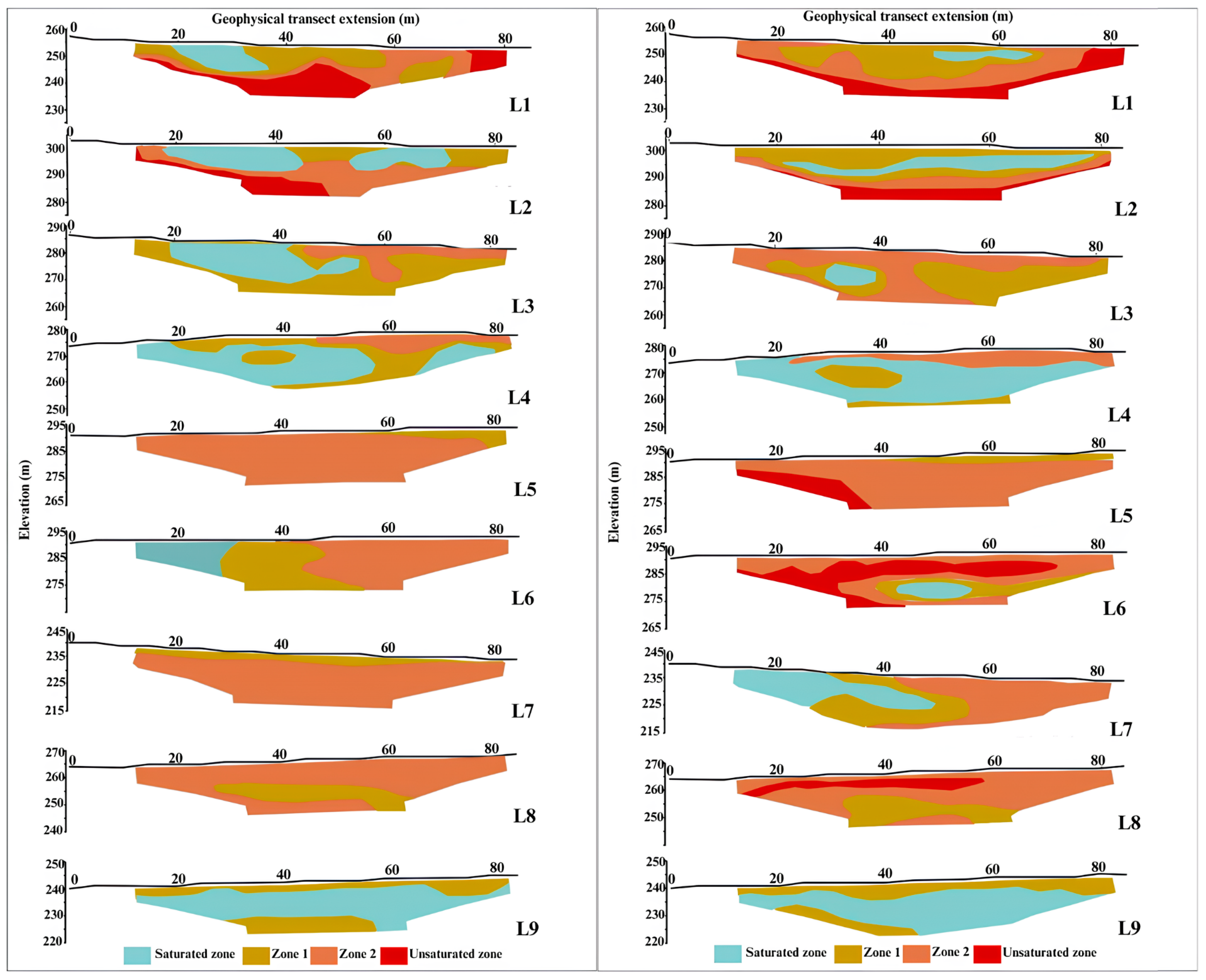
3.2. Subsurface Characterization: Groundwater

Three profiles per watershed were characterized geophysically at the end of the dry and wet periods. The color scale ranged from 33 to 11,605 Ω·m, with root mean square (RMS) errors ranging from 7.1% to 39.5% for the wet period and 5% to 34% for the dry period (Figure 3). Most errors were observed for lower resistivity values, while in transects with higher resistivity values, the errors were lower, thus requiring less data smoothing.
Electrical resistivity profiles (Figure 4) and quantification zones (Table 2) were created for the nine transects. During the evaluation period, an expansion of the saturated zone was observed in transects L4 and L7 in the Es-W watershed. These changes in features, boundaries, and geometry are closely linked to the soil profile water balance (Figure 2). The model with the lowest RMS error sometimes indicates large and unrealistic changes in resistivity values [43] and may not always be the best model from a geological perspective. The most prudent approach is to select the model interactively, after which the RMS error does not change significantly. This may apply to sections where resistivity values were not consistently low.
The Es-W watershed (transects 4 and 7) experienced water deficits in November 2019. Consequently, due to the evapotranspiration demand not being satisfied because of water deficit (DEF), the water demand of eucalyptus was likely higher, resulting in a reduced amount of soil water. In transect 9, the zones were similar across both fields (Figure 5). The soil saturated zone reduced from the wet to the dry period in all transects evaluated in the G-W watershed (Table 2). This decrease is potentially explained by water deficits observed in March and April during the dry period.
In Es-W, despite an increase in the saturated zone for profiles L4 and L7 and variations in the proportions of zones 1 and 2, there was no unsaturated zone in these profiles. In L5, the occurrence of an unsaturated zone was observed only in the measurements for the dry period, ranging from 0 to 12.9%. Similar behavior occurred in Eb-W, where the unsaturated zone ranged from 0 to 34.9% in L6 and from 0 to 13.6% in L8. The presence of an unsaturated zone during the dry period resulted from the contribution of percentages previously representing zone 2, characterized by medium to fine unsaturated sandstones.
Overall, the highest water content observed among watersheds was in the G-W for the wet and dry periods. Groundwater variations among the forest watersheds were not as clear as the observed surface water variations from the water balance estimation. During the dry period, unsaturated zones appeared in two profiles of Eb-W and only one of Es-W. However, saturated zones were observed in two profiles of Es-W (64.6 and 29.5%) and Eb-W (63.6 and 6.9%).
Despite the high accumulated rainfall of 199.9 mm in May 2020, this precipitation was insufficient to expand the soil saturated zone, as observed in transects 1–3 (Figure 4), due to drought conditions in the preceding months. In the same area, Ferreto et al. [4] observed the occurrence of soil water replenishment during autumn and winter due to reduced plant growth, along with increased water consumption by plants during summer, which is the period of higher vegetative growth. This phenomenon was also observed by Almeida et al. [50], with greater soil water depletion during summer attributed to high evapotranspiration resulting from higher vapor pressure deficits and high solar radiation.
Water absorption by plant roots depends on water potential, as roots absorb more water when the water potential in the root zone is more negative compared to the soil solution. This is especially true with a more extensive root system [51] and may explain the saturated zone in the root zone of eucalyptus (Figure 5 and Figure 6). When water availability in the environment is insufficient, plants experience water deficits. Christina et al. [52] suggest that eucalyptus crops, after canopy closure, draw water from the capillary fringe, and the soil-saturated zone acts as an additional water source that was replenished within the first two years after clear-cutting and was only partially used after tree canopy closure.
Groundwater in forest watersheds decreased compared to those in grassland watersheds. This is justified by the plant’s ability in forest watersheds to acquire water from deeper roots and soil layers during dry periods. This behavior may have occurred mainly in profiles L5, L6, and L8, where there was no unsaturated zone during the wet periods, which appeared after the rainfall reduction during the growing season. Predicting root water uptake is complex due to the variability of influencing factors. Despite soil and environmental conditions, plant species tend to regulate this behavior. For some species, plants tend to decrease transpiration when the topsoil dries, even when the groundwater is available, but for others, transpiration is maintained through water uptake from bedrock fractures [32,53]. The combination of water balance estimation and ERT better described the hydrological dynamics in paired watersheds with different land uses.

4. Conclusions

The study objective was to assess whether eucalyptus plantations reduce groundwater levels in paired subtropical watersheds compared to grasslands. Geophysical methods constituted a valuable alternative for collecting data in forested and grassland areas, allowing for the characterization of different subsurface geometries and aiding in water balance estimations. Through water balance, variations in interception, evapotranspiration, and runoff in forested watersheds were identified in comparison with the grassland watershed. These differences result from the physiological characteristics of each vegetation cover (e.g., leaf area, root system, and stomatal efficiency) and water availability (precipitation and soil water). During winter, with reduced crop growth due to higher moisture and lower incidence of sunlight and temperature, excess water is stored in the soil and recharging groundwater, while during summer, plants utilize water from deeper zones, e.g., from the saturated subsoil, due to greater evapotranspiration.

Author Contributions

Conceptualization, É.E.B.d.S. and J.M.R.; methodology, É.E.B.d.S., J.M.R., P.D.d.C.K., É.D.E. and M.M.Z.; formal analysis, É.E.B.d.S. and J.M.R.; investigation, all; resources, E.F.d.A.; data curation, É.E.B.d.S. and E.F.d.A.; writing—original draft preparation, É.E.B.d.S. and F.d.B.; writing—review and editing, F.d.B. and J.M.R.; supervision, J.M.R. and P.D.d.C.K.; project administration, J.M.R., É.D.E. and P.D.d.C.K.; funding acquisition, J.M.R. All authors have read and agreed to the published version of the manuscript.

Funding

We thank Coordenação de Aperfeiçoamento de Pessoal de Nível Superior (Capes)—Finance code 001; RITES-FAPERGS “Low Carbon Agriculture Adapted to Climate Changes in Rio Grande do Sul” project (22/2551-0000392-3); INCT Low Carbon Emission Agriculture (CNPq 406635/2022-6); Geology group of the Universidade Federal do Pampa; and CMPC Cellulose Riograndense.

Data Availability Statement

The data presented in this study are available on request from the corresponding author.

Acknowledgments

We thank Maximilian Fries, from Universidade Federal do Pampa, Thais Palumbo da Silva and Gabriel D’Avila Fernandes, from UFSM, and José Carlos de Deus Junior, from CMPC, for their assistance with equipment, fieldwork and software, or data provision.

Conflicts of Interest

Author Elias Frank de Araujo was employed by the company CMPC Celulose Riograndense. The remaining authors declare that the research was conducted in the absence of any commercial or financial relationships that could be construed as a potential conflict of interest.

References

  1. WWF. Forests and Climate: REDD+ at a Crossroads: Living Forests Report: Chapter 3. In Living Forests Report; WWF: Gland, Switzerland, 2011. [Google Scholar]
  2. Maeda, S.; Medrado, M.J.S. Plantações Florestais Comerciais e o Solo. In Plantações Florestais: Geração de Benefícios com Baixo Impacto Ambiental; Embrapa: Brasília, Brazil, 2017; pp. 21–29. [Google Scholar]
  3. Ferreto, D.O.C.; Reichert, J.M.; Cavalcante, R.B.L.; Srinivasan, R. Rainfall Partitioning in Young Clonal Plantations Eucalyptus Species in a Subtropical Environment, and Implications for Water and Forest Management. Int. Soil Water Conserv. Res. 2021, 9, 474–484. [Google Scholar] [CrossRef]
  4. Ferreto, D.O.C.; Reichert, J.M.; Cavalcante, R.B.L.; Srinivasan, R. Water Budget Fluxes in Catchments under Grassland and Eucalyptus Plantations of Different Ages. Can. J. For. Res. 2021, 51, 513–523. [Google Scholar] [CrossRef]
  5. Pirard, R.; Dal Secco, L.; Warman, R. Do Timber Plantations Contribute to Forest Conservation? Environ. Sci. Policy 2016, 57, 122–130. [Google Scholar] [CrossRef]
  6. Kröger, M. The Expansion of Industrial Tree Plantations and Dispossession in Brazil. Dev. Change 2012, 43, 947–973. [Google Scholar] [CrossRef]
  7. Dodet, M.; Collet, C. When Should Exotic Forest Plantation Tree Species Be Considered as an Invasive Threat and How Should We Treat Them? Biol. Invasions 2012, 14, 1765–1778. [Google Scholar] [CrossRef]
  8. Lorentz, K.A.; Minogue, P.J. Exotic Eucalyptus Plantations in the Southeastern US: Risk Assessment, Management and Policy Approaches. Biol. Invasions 2015, 17, 1581–1593. [Google Scholar] [CrossRef]
  9. Vance, E.D.; Loehle, C.; Wigley, T.B.; Weatherford, P. Scientific Basis for Sustainable Management of Eucalyptus and Populus as Short-Rotation Woody Crops in the U.S. Forests 2014, 5, 901–918. [Google Scholar] [CrossRef]
  10. Gush, M.B.; Scott, D.F.; Jewitt, G.P.W.; Schulze, R.E.; Hallowes, L.A.; Görgens, A.H.M. A New Approach to Modelling Streamflow Reductions Resulting from Commercial Afforestation in South Africa. S. Afr. For. J. 2002, 2002, 27–36. [Google Scholar] [CrossRef]
  11. Cademus, R.; Escobedo, F.J.; McLaughlin, D.; Abd-Elrahman, A. Analyzing Trade-Offs, Synergies, and Drivers among Timber Production, Carbon Sequestration, and Water Yield in Pinus elliotii Forests in Southeastern USA. Forests 2014, 5, 1409–1431. [Google Scholar] [CrossRef]
  12. Ferraz, S.F.B.; Lima, W.d.P.; Rodrigues, C.B. Managing Forest Plantation Landscapes for Water Conservation. For. Ecol. Manag. 2013, 301, 58–66. [Google Scholar] [CrossRef]
  13. Baumhardt, E. Hidrologia de Bacia de Cabeceira com Eucaliptocultura e Campo Nativo na Região da Campanha Gaúcha. Doctoral Dissertation, Universidade Federal de Santa Maria, Santa Maria, Brazil, 2014. [Google Scholar]
  14. Reichert, J.M.; Rodrigues, M.F.; Peláez, J.J.Z.; Lanza, R.; Minella, J.P.G.; Arnold, J.G.; Cavalcante, R.B.L. Water Balance in Paired Watersheds with Eucalyptus and Degraded Grassland in Pampa Biome. Agric. For. Meteorol. 2017, 237, 282–295. [Google Scholar] [CrossRef]
  15. Rodrigues, M.F.; Reichert, J.M.; Burrow, R.A.; Flores, E.M.M.; Minella, J.P.G.; Rodrigues, L.A.; Oliveira, J.S.S.; Cavalcante, R.B.L. Coarse and Fine Sediment Sources in Nested Watersheds with Eucalyptus Forest. Land Degrad. Dev. 2018, 29, 2237–2253. [Google Scholar] [CrossRef]
  16. Ebling, É.D.; Reichert, J.M.; Zuluaga Peláez, J.J.; Rodrigues, M.F.; Valente, M.L.; Lopes Cavalcante, R.B.; Reggiani, P.; Srinivasan, R. Event-Based Hydrology and Sedimentation in Paired Watersheds under Commercial Eucalyptus and Grasslands in the Brazilian Pampa Biome. Int. Soil Water Conserv. Res. 2021, 9, 180–194. [Google Scholar] [CrossRef]
  17. Dos Santos, K.F.; Reichert, J.M. Best Tillage Practices for Eucalyptus Growth and Productivity: A Review on the Brazilian Experience. Rev. Bras. Cienc. do Solo 2022, 46, e0210091. [Google Scholar] [CrossRef]
  18. Reichert, J.M.; Prevedello, J.; Gubiani, P.I.; Vogelmann, E.S.; Reinert, D.J.; Consensa, C.O.B.; Soares, J.C.W.; Srinivasan, R. Eucalyptus Tree Stockings Effect on Water Balance and Use Efficiency in Subtropical Sandy Soil. For. Ecol. Manag. 2021, 497, 119473. [Google Scholar] [CrossRef]
  19. Cavalli, J.P.; Reichert, J.M.; Rodrigues, M.F.; de Araújo, E.F. Composition and Functional Soil Properties of Arenosols and Acrisols: Effects on Eucalyptus Growth and Productivity. Soil Tillage Res. 2020, 196, 104439. [Google Scholar] [CrossRef]
  20. de Bastos, F.; Reichert, J.M.; Minella, J.P.G.; Rodrigues, M.F. Strategies for Identifying Pollution Sources in a Headwater Catchment Based on Multi-Scale Water Quality Monitoring. Environ. Monit. Assess. 2021, 193, 169. [Google Scholar] [CrossRef]
  21. Conant, B.; Robinson, C.E.; Hinton, M.J.; Russell, H.A.J. A Framework for Conceptualizing Groundwater-Surface Water Interactions and Identifying Potential Impacts on Water Quality, Water Quantity, and Ecosystems. J. Hydrol. 2019, 574, 609–627. [Google Scholar] [CrossRef]
  22. Chandra, S.; Dewandel, B.; Dutta, S.; Ahmed, S. Geophysical Model of Geological Discontinuities in a Granitic Aquifer: Analyzing Small Scale Variability of Electrical Resistivity for Groundwater Occurrences. J. Appl. Geophys. 2010, 71, 137–148. [Google Scholar] [CrossRef]
  23. McLachlan, P.J.; Chambers, J.E.; Uhlemann, S.S.; Binley, A. Geophysical Characterisation of the Groundwater–Surface Water Interface. Adv. Water Resour. 2017, 109, 302–319. [Google Scholar] [CrossRef]
  24. Mansour, K.; Omar, K.; Ali, K.; Abdel Zaher, M. Geophysical Characterization of the Role of Fault and Fracture Systems for Recharging Groundwater Aquifers from Surface Water of Lake Nasser. NRIAG J. Astron. Geophys. 2018, 7, 99–106. [Google Scholar] [CrossRef]
  25. Knight, A.C.; Werner, A.D.; Irvine, D.J. Combined Geophysical and Analytical Methods to Estimate Offshore Freshwater Extent. J. Hydrol. 2019, 576, 529–540. [Google Scholar] [CrossRef]
  26. Ezema, O.K.; Ibuot, J.C.; Obiora, D.N. Geophysical Investigation of Aquifer Repositories in Ibagwa Aka, Enugu State, Nigeria, Using Electrical Resistivity Method. Groundw. Sustain. Dev. 2020, 11, 100458. [Google Scholar] [CrossRef]
  27. Parsekian, A.D.; Singha, K.; Minsley, B.J.; Holbrook, W.S.; Slater, L. Multiscale Geophysical Imaging of the Critical Zone. Rev. Geophys. 2015, 53, 1–26. [Google Scholar] [CrossRef]
  28. Chambers, J.E.; Gunn, D.A.; Wilkinson, P.B.; Meldrum, P.I.; Haslam, E.; Holyoake, S.; Kirkham, M.; Kuras, O.; Merritt, A.; Wragg, J. 4D Electrical Resistivity Tomography Monitoring of Soil Moisture Dynamics in an Operational Railway Embankment. Near Surf. Geophys. 2014, 12, 61–72. [Google Scholar] [CrossRef]
  29. de Oliveira, M.V.G.; Moreira, C.A.; Netto, L.G.; Nascimento, M.M.P.F.; Sampaio, B.V. Geophysical and Geological Surveys to Understand the Hydrogeological Behavior in an Outcrop Area of the Guarani Aquifer System, in Brazil. Environ. Chall. 2022, 6, 100448. [Google Scholar] [CrossRef]
  30. Moreira, C.A.; Helene, L.P.I.; Rosa, F.T.G.; Hansen, M.A.F.; Malagutti Filho, W.; Dourado, J.C. Comparative Analysis among Electrical Resistivity Tomography Arrays in the Reconnaissance of Flow Structure in Fractures Aquifer in Caçapava Do Sul (RS). Pesqui. Geocienc. 2019, 46, e0710. [Google Scholar] [CrossRef]
  31. Myhre, G.; Alterskjær, K.; Stjern, C.W.; Hodnebrog; Marelle, L.; Samset, B.H.; Sillmann, J.; Schaller, N.; Fischer, E.; Schulz, M.; et al. Frequency of Extreme Precipitation Increases Extensively with Event Rareness under Global Warming. Sci. Rep. 2019, 9, 16063. [Google Scholar] [CrossRef]
  32. Tfwala, C.M.; van Rensburg, L.D.; Bello, Z.A. Groundwater Contribution to Transpiration of Trees under Wet and Dry Soil Conditions. Irrig. Drain. 2021, 70, 42–51. [Google Scholar] [CrossRef]
  33. de Bastos, F.; Carlos, J.; Júnior, D.D.; Ebling, É.D.; Neumann, M.; Reichert, J.M.; Neumann, M. Efficiency of Water Use by Eucalyptus spp. for Water Conservation and Sustainable Forest Production. Hydrol. Sci. J. 2024, 69, 844–860. [Google Scholar] [CrossRef]
  34. Alvares, C.A.; Stape, J.L.; Sentelhas, P.C.; De Moraes Gonçalves, J.L.; Sparovek, G. Köppen’s Climate Classification Map for Brazil. Meteorol. Z. 2013, 22, 711–728. [Google Scholar] [CrossRef] [PubMed]
  35. Moreno, J.A. Clima Do Rio Grande Do Sul. In Boletim Geográfico do Estado do Rio Grande do Sul; Secretaria de Planejamento, Governança e Gestão: Porto Alegre, Brazil, 1961; Volume 11, pp. 2446–7251. [Google Scholar]
  36. Reichert, J.M.; de Deus Junior, J.C.; Borges Junior, N.; Cavalcante, R.B.L. Experimental Catchments in the Pampa Biome: Database on Hydrology in Grasslands and Eucalyptus Plantations in Subtropical Brazil. Hydrol. Process. 2021, 35, e14285. [Google Scholar] [CrossRef]
  37. USDA—United States Department of Agriculture. Keys to Soil Taxonomy; USDA: Washington, DC, USA, 2014.
  38. Dos Santos, H.G.; Jacomine, P.K.T.; Anjos, L.H.C.; Oliveira, V.Á.; Oliveira, J.B.; Coelho, M.R.; Lumbreras, J.F.; Cunha, T.J.F. Sistema Brasileiro de Classificação de Solos, 3rd ed.; Empresa Brasileira de Pesquisa Agropecuária (EMBRAPA): Brasília, Brazil, 2013; 353p, ISBN 85-85864-19-2. [Google Scholar]
  39. Allen, R.G.; Pereira, L.S.; Raes, D.; Smith, M. Crop Evapotranspiration—Guidelines for Computing Crop Water Requirements—FAO Irrigation and Drainage Paper 56; FAO: Rome, Italy, 1998. [Google Scholar] [CrossRef]
  40. Thornthwaite, C.W.; Mather, J.R. The Water Balance; Drexel Institute of Technology—Laboratory of Climatology: Centerton, NJ, USA, 1955. [Google Scholar]
  41. ABNT NBR 15.935; Investigações Ambientais—Aplicação de Métodos Geofísicos. ABNT: Rio de Janeiro, Brazil, 2011.
  42. Degroot-Hedlin, C.; Constable, S. Occam’s Inversion to Generate Smooth, Two-Dimensional Models from Magnetotelluric Data. Geophysics 1990, 55, 1613–1624. [Google Scholar] [CrossRef]
  43. Loke, M. Rapid 2-D Resistivity & IP Inversion Using the Least-Squares Method; Geotomo Software: Penang, Malaysia, 2019. [Google Scholar]
  44. Resende, R.T.; Soares, A.A.V.; Forrester, D.I.; Marcatti, G.E.; dos Santos, A.R.; Takahashi, E.K.; e Silva, F.F.; Grattapaglia, D.; Resende, M.D.V.; Leite, H.G. Environmental Uniformity, Site Quality and Tree Competition Interact to Determine Stand Productivity of Clonal Eucalyptus. For. Ecol. Manag. 2018, 410, 76–83. [Google Scholar] [CrossRef]
  45. de Mattos, E.M.; Binkley, D.; Campoe, O.C.; Alvares, C.A.; Stape, J.L. Variation in Canopy Structure, Leaf Area, Light Interception and Light Use Efficiency among Eucalyptus Clones. For. Ecol. Manag. 2020, 463, 118038. [Google Scholar] [CrossRef]
  46. Migacz, I.P.; Raeski, P.A.; de Almeida, V.P.; Raman, V.; Nisgoski, S.; de Muniz, G.I.B.; Farago, P.V.; Khan, I.A.; Budel, J.M. Comparative Leaf Morpho-Anatomy of Six Species of Eucalyptus Cultivated in Brazil. Rev. Bras. Farmacogn. 2018, 28, 273–281. [Google Scholar] [CrossRef]
  47. Dresel, P.E.; Dean, J.F.; Perveen, F.; Webb, J.A.; Hekmeijer, P.; Adelana, S.M.; Daly, E. Effect of Eucalyptus Plantations, Geology, and Precipitation Variability on Water Resources in Upland Intermittent Catchments. J. Hydrol. 2018, 564, 723–739. [Google Scholar] [CrossRef]
  48. Pinheiro, R.C.; de Deus Junior, J.C.; Nouvellon, Y.; Campoe, O.C.; Stape, J.L.; Aló, L.L.; Guerrini, I.A.; Jourdan, C.; Laclau, J.P. A Fast Exploration of Very Deep Soil Layers by Eucalyptus Seedlings and Clones in Brazil. For. Ecol. Manag. 2016, 366, 143–152. [Google Scholar] [CrossRef]
  49. de Barros Ferraz, S.F.; Rodrigues, C.B.; Garcia, L.G.; Alvares, C.A.; de Paula Lima, W. Effects of Eucalyptus Plantations on Streamflow in Brazil: Moving beyond the Water Use Debate. For. Ecol. Manag. 2019, 453, 117571. [Google Scholar] [CrossRef]
  50. Almeida, A.C.; Soares, J.V.; Landsberg, J.J.; Rezende, G.D. Growth and Water Balance of Eucalyptus Grandis Hybrid Plantations in Brazil during a Rotation for Pulp Production. For. Ecol. Manag. 2007, 251, 10–21. [Google Scholar] [CrossRef]
  51. Dos Reis, G.G.; Reis, M.G.F. Fisiologia da Brotação de Eucalipto com Ênfase nas Suas Relações Hídricas; IPEF—Instituto de Pesquisas e Estudos Florestais: Piracicaba, Brazil, 1997. [Google Scholar]
  52. Christina, M.; Nouvellon, Y.; Laclau, J.P.; Stape, J.L.; Bouillet, J.P.; Lambais, G.R.; le Maire, G. Importance of Deep Water Uptake in Tropical Eucalypt Forest. Funct. Ecol. 2017, 31, 509–519. [Google Scholar] [CrossRef]
  53. Eliades, M.; Bruggeman, A.; Lubczynski, M.W.; Christou, A.; Camera, C.; Djuma, H. The Water Balance Components of Mediterranean Pine Trees on a Steep Mountain Slope during Two Hydrologically Contrasting Years. J. Hydrol. 2018, 562, 712–724. [Google Scholar] [CrossRef]
Figure 1. Study area with three watersheds predominantly under Eucalyptus benthamii (Eb-W), Eucalyptus saligna (Es-W), and grassland (G-W), showing the transects in the watersheds: G-W (L1 to L3), Es-W (L4, L5 and L7), and Eb-W (L6, L8, and L9) for electrical resistivity measurements, where each transect had a length of about 90 m and a dipole–dipole arrangement with an electrode spacing of 5 m.
Water 16 02191 g001
Figure 2. Sequential water balance, adapted from Thornthwaite and Mather (1955), and monitoring flow levels for Eb-W (left), Es-W (center), and G-C (right). The lower piezometers were located at elevations of 243.5, 236.4, and 260.8 m a.s.l. for Eb-W, Es-W, and G-C, respectively, while the upper ones were at elevations of 298.3, 266.3, and 291.8 m a.s.l., respectively. Data used until 15 June 2020.
Water 16 02191 g002
Figure 3. Electrical resistivity values (Ω·m) for the transects evaluated at the end of the wet period on 19 November 2019 (left) and at the end of the dry period on 04 June 2020 (right).
Water 16 02191 g003
Figure 4. Zoning of transects evaluated at the end of the wet (left) and dry periods (right).
Water 16 02191 g004
Figure 5. Zoning of transect 9 (L9) evaluated at the end of the wet (a) and dry periods (b).
Water 16 02191 g005
Figure 6. Zoning of transect 4 (L4) evaluated at the end of the wet (a) and dry periods (b).
Water 16 02191 g006
Table 1. Water balance components—rainfall (P), runoff (Q), water intercepted by vegetation (Int), and soil evapotranspiration (ETa)—for the wet period (5 June 2019 to 19 November 2019) and the dry period (20 November 2019 to 4 June 2020), both consisting of 197 days for the Eucalyptus benthamii (Eb-W), Eucalyptus saligna (Es-W), and grassland (G-W) watersheds.
VariableEb-WEs-WG-W
WetDryWetDryWetDry
P (mm)1098.50478.51098.50478.51098.50478.5
Q (mm)225.822.7 *229.8 **66.6649.6 ***84.7 ***
Int (mm)248.4108.3356.1154.9149.465.1
ETa (mm)624.3347.5512.6257299.5328.7
Notes: * Only from 11 July 2019 to 4 December 2019; ** From 23 July 2019 to 20 August 2019; *** From 26 July 2019 to 29 July 2019 and from 30 November 2019 to 19 December 2019.
Table 2. Relative proportion (%) of saturated zones, zones 1 and 2, and the unsaturated zone for each of the nine transects at the end of the wet and dry periods for the Eucalyptus benthamii (Eb-W), Eucalyptus saligna (Es-W), and grassland (G-W) watersheds.
End of Wet Period (19 November 2019)End of Dry Period (4 June 2020)
Transection 1 (%) G-WTransection 1 (%) G-W
Saturated zone 12.7Saturated zone 5.3
Zone 1 29.4Zone 1 33.0
Zone 2 28.3Zone 2 37.4
Unsaturated zone 29.6Unsaturated zone 24.3
Transection 2 (%) G-WTransection 2 (%) G-W
Saturated zone 33.9Saturated zone 22.2
Zone 1 15.5Zone 1 40.3
Zone 2 35.8Zone 2 21.5
Unsaturated zone 14.8Unsaturated zone 16.0
Transection 3 (%) G-WTransection 3 (%) G-W
Saturated zone 33.8 Saturated zone 5.8
Zone 1 47.5Zone 1 40.3
Zone 2 18.7 Zone 2 53.9
Unsaturated zone -Unsaturated zone -
Transection 4 (%) Es-WTransection 4 (%) Es-W
Saturated zone 53.3 Saturated zone 64.6
Zone 1 32.1 Zone 1 15.0
Zone 2 14.6 Zone 2 20.4
Unsaturated zone -Unsaturated zone -
Transection 5 (%) Es-WTransection 5 (%) Es-W
Saturated zone -Saturated zone -
Zone 1 6.8 Zone 1 9.6
Zone 2 93.2Zone 2 77.5
Unsaturated zone -Unsaturated zone 12.9
Transection 6 (%) Eb-WTransection 6 (%) Eb-W
Saturated zone -Saturated zone 6.9
Zone 1 13.7 Zone 1 13.7
Zone 2 86.3 Zone 2 44.5
Unsaturated zone -Unsaturated zone 34.9
Transection 7 (%) Es-WTransection 7 (%) Es-W
Saturated zone 18.5 Saturated zone 29.5
Zone 1 33.7 Zone 1 26.9
Zone 2 47.8 Zone 2 43.6
Unsaturated zone -Unsaturated zone -
Transection 8 (%) Eb-WTransection 8 (%) Eb-W
Saturated zone -Saturated zone -
Zone 1 21.0Zone 1 22.5
Zone 2 79.0 Zone 2 63.9
Unsaturated zone -Unsaturated zone 13.6
Transection 9 (%) Eb-WTransection 9 (%) Eb-W
Saturated zone 64.7 Saturated zone 63.6
Zone 1 35.3Zone 1 36.4
Zone 2 -Zone 2 -
Unsaturated zone -Unsaturated zone -
Disclaimer/Publisher’s Note: The statements, opinions and data contained in all publications are solely those of the individual author(s) and contributor(s) and not of MDPI and/or the editor(s). MDPI and/or the editor(s) disclaim responsibility for any injury to people or property resulting from any ideas, methods, instructions or products referred to in the content.

