
Refined Reservoir Routing (RRR) and Its Application to Atmospheric Carbon Dioxide Balance


Department of Water Resources and Environmental Engineering, School of Civil Engineering, National Technical University of Athens, 157 72 Zographou, Greece
Water 2024, 16(17), 2402; https://doi.org/10.3390/w16172402
Submission received: 13 May 2024
/
Revised: 3 August 2024
/
Accepted: 23 August 2024
/
Published: 26 August 2024
Abstract
:Reservoir routing has been a routine procedure in hydrology, hydraulics and water management. It is typically based on the mass balance (continuity equation) and a conceptual equation relating storage and outflow. If the latter is linear, then there exists an analytical solution of the resulting differential equation, which can directly be utilized to find the outflow from known inflow and to obtain macroscopic characteristics of the process, such as response and residence times, and their distribution functions. Here we refine the reservoir routing framework and extend it to find approximate solutions for nonlinear cases. The proposed framework can also be useful for climatic tasks, such as describing the mass balance of atmospheric carbon dioxide and determining characteristic residence times, which have been an issue of controversy. Application of the theoretical framework results in excellent agreement with real-world data. In this manner, we easily quantify the atmospheric carbon exchanges and obtain reliable and intuitive results, without the need to resort to complex climate models. The mean residence time of atmospheric carbon dioxide turns out to be about four years, and the response time is smaller than that, thus opposing the much longer mainstream estimates.
What is more I loved, and still do love, mathematics for itself as not allowing room for hypocrisy or vagueness, my two pet aversions.Stendhal [1] (p. 111).
1. Introduction
Thanks to their links with real-world problems and their engineering approach in seeking rational solutions to them, hydrology and hydraulics have ever been in close contact with reality. This has prevented them from practicing hypocrisy and vagueness, much like in mathematics (cf. the epigram above). Historically, the solutions to real-world problems preceded the development of hydrology and hydraulics as sciences and thus could not be based on scientific knowledge. Rather, they were based on common sense, which historically has provided the foundation of philosophical and scientific knowledge, while in recent decades, it tends to be abandoned in favor of what euphemistically has been called “political correctness”.
Among the solutions to real-world problems, the technology of storage, implemented by cisterns at a small scale and reservoirs at dammed rivers at a large scale, has been most determinant. Perhaps the first dam with a reservoir storing water was that in Jawa, in the desert of Northeastern Jordan, a 5 m high and 80 m long dam dated between 3500 and 3400 BC [2]. Another prehistoric example is the so-called Sadd el Kafara dam in Wadi Garawi, about 50 km southeast of Cairo, dated into the old kingdom of Egypt, around 2650 BC [3].
Storage facilities for surpluses of goods, in particular grains, to be consumed in periods of deficit, preceded those for water. Granaries date as far back as 9500 BC in the Jordan Valley, coinciding with the dawn of agriculture, and they were initially at the household scale, later expanding to larger scales for collective storage of grain [4].
We may speculate that this type of storage, whether for water or grain, was for seasonal (intra-annual) regulation and is far different from modern facilities for overyear regulation. Yet we have written information about the latter type of regulation, which is necessary to deal with famines, in the biblical story of Joseph and the pharaoh’s dream of the seven fat and the seven skinny cows. The famine, which was predicted by Joseph in his interpretation of the pharaoh’s dream, indeed occurred, but Egypt was prepared for it [5].
Bell [6] and Said [7] confirm this biblical story and date it to an uncertain number of years preceding 1740 BC. Specifically, Bell [6] links this story with an inscription in the tomb of Sobek-nakht, which was decorated in the three-year reign of Sobekhotep III, just prior to ca. 1740, and reads as follows: “I was a man who protected the afflicted against the powerful […] who supplied the granaries of the god […] who summoned his entire energy every time he saw an insufficient flood”. She also refers to another (undated) tomb inscription, which reads, “I gave grain to the entire country, I saved my town from famine […] no one has done what I did”.
This biblical story is of great hydrological and climatic importance, as it is perhaps the oldest text referring to a long-lasting drought, as well as to the natural behavior of clustering in time of similar events (such as dry or wet years), which in recent times was quantified by Hurst [8] in 1951. Mandelbrot and Wallis [9] used the term Joseph effect for this behavior, which today is more often called Hurst-Kolmogorov dynamics [10]. The importance of the story extends to good management practices, in which the storage of goods (in this case in granaries) during periods of abundance can mitigate the adverse consequences in periods of shortage.
Yet storage is not a human invention, because nature uses it extensively. Numerous natural processes include storage, and their modeling needs to properly represent it. On the other hand, the need for the design and management of human storage facilities, particularly water reservoirs, has enabled deeper insights and more concrete knowledge on modeling storage and the related processes. This modeling typically follows a systems approach, with an input (inflow), an output (outflow), and a state variable (stored quantity). These three quantities are interlinked with a first principle, i.e., mass conservation, implemented as a linear differential or a difference equation. This, however, does not suffice for complete modeling. One more equation is needed. In detailed physical modeling, this can be offered by another physical principle, such as conservation of momentum, but in macroscopic modeling, this is not possible, and the second equation is macroscopic with some conceptual or statistical meaning, depending on the nature of the system. In particular, if this second equation is a linear relationship between inflow and storage, then there exists an analytical solution of the resulting differential equation, which can be directly utilized to find the outflow from the known inflow and to obtain macroscopic characteristics of the process, such as response and residence times and their distribution functions. If that equation is nonlinear, then only special cases admit an analytical solution.
Here, the reservoir routing framework is revisited, streamlined, and extended to find approximate solutions for nonlinear cases (Section 2). Furthermore, this framework, developed under the name Refined Reservoir Routing (RRR), is applied to a topical issue of climatic interest, the mass balance of atmospheric carbon dioxide (Section 4). Before that (in Section 3), the particulars of the problem of atmospheric carbon dioxide storage are discussed, along with a summary of the complex established approach, which presents substantial differences from the simple RRR approach. The RRR framework readily allows the determination of characteristic residence times, which have been an issue of controversy (Section 5). It is concluded (Section 6) that the application of the RRR framework results in excellent agreement with real-world data. In this manner, it easily quantifies the atmospheric carbon exchanges and produces reliable and intuitive results, without the need to resort to complex climate models.
It is worth emphasizing that the atmospheric carbon dioxide balance, like the water balance, is governed by geophysical processes, despite the common perception that it is determined by human emissions from the burning of fossil fuels. The latter represent only 4% of total emissions [11], and in this respect, they are similar to human emissions of water vapor, whose percentage is of the same order of magnitude [12,13,14,15]. In global hydrology, we usually neglect the human emissions part, although we certainly consider it in local studies related to irrigation. The opposite is thought in climate studies, where human emissions are seen as the cornerstone of the climate edifice. However, this is not due to the importance of human emissions but has rather been dictated by non-scientific influences [15]. Geophysically driven emissions of both carbon dioxide and water vapor are closely linked to each other and to the biosphere processes.
Specifically, during photosynthesis, plants absorb both CO2 and H2O, producing organic matter. The water availability drives the uptake of CO2 through stomata, creating an interconnected cycle of gas exchange. In addition, both plants and animals respire, emitting CO2 and H2O, while plants also transpire. These processes determine the inflow of both CO2 and H2O to the atmosphere. Furthermore, decomposers break down organic material, releasing CO2, while water facilitates the breakdown of organic compounds, influencing the decomposition rates and thus CO2 emissions. The hydrological cycle influences plant growth by providing the water needed for photosynthesis, thereby driving CO2 absorption. Furthermore, both CO2 and H2O affect the climate, as both are greenhouse gases, with water being the determinant one, as, in addition to its much larger absorption of longwave radiation, it is also responsible for clouds, which also absorb radiation [15].
Of these two, we opt to study the atmospheric CO2 balance for three reasons:
- Its “lumping” in a systems approach is direct, because its concentration varies slowly, while that of atmospheric water varies dramatically with time, geographic location, and altitude.
- As we will see below, there is controversy about the atmospheric CO2 budget, reflecting incomplete understanding and quantification of the processes, which the simple RRR framework may shed light on.
- Exporting a methodological framework developed in hydrology to the study of climate may be beneficial to both hydrology and climatology and may demonstrate the potential and usefulness of hydrology in climate research.
2. Theoretical Analysis
2.1. System Components and Determination of Their Temporal Evolution
We consider a system that can be represented as a reservoir, with input , output , and storage . These three quantities are connected by the continuity equation, which expresses the conservation of mass and is written in differential form as
It can be seen that in the systems approach we follow, the continuity equation is unidimensional. No extensions for more dimensions are required. In hydrosystems, the inflow is typically the upstream flow discharge, the outflow is the downstream flow discharge or a reservoir spill, and they are usually expressed in terms of volumes instead of masses. (However, unless we deal with uncompressible fluids, we should stick with mass units.) The reservoir could be a real one, upstream of a dam, but the use of imaginary reservoirs is not uncommon. For example, an entire catchment is often represented as a single imaginary reservoir with the inflow being the precipitation [10,16] or as a cascade of reservoirs [17], in which outputs from upstream reservoirs are inputs to the downstream reservoirs in the cascade. Similar representations may be appropriate for groundwater stored in aquifers [18].
Storage, however, is not limited to locally resolved processes of surface- or ground-water. The global hydrological cycle can be viewed in terms of mass exchange, with the main storage being the oceans but with the atmosphere having a crucial role when evaporation and precipitation are studied [19]. Modeling of the carbon cycle can also be made in a similar setting, as will be shown in Section 4.
The typical problem is to determine the outflow for known inflow . To fully describe the transformation of inflow to outflow, we need one more equation. The solution of the two equations is commonly known as reservoir routing. In hydrology and hydraulics, we usually construct the second equation by means of stage–discharge and stage–storage relationships. Different equations can be formulated, depending on the system dynamics, but the following power type (combined) equation is representative for most problems:
where is a dimensionless parameter (exponent), and and are parameters with units of mass and mass flow, respectively. These are necessary to make the equation physically (dimensionally) consistent and here will be regarded to be the initial conditions (at time zero, i.e., and , respectively). Notice that these parameters are not unique; for example, we can multiply and by and , respectively, and get another pair of valid parameters.
It is well known that when , we get a first-order linear differential equation with constant coefficients, i.e.,
where is a characteristic residence time, whose meaning will be discussed below. This admits a closed solution:
This case () is known as the linear reservoir [20,21,22,23,24,25], and the fact that it admits a general analytical solution makes it a useful tool. We will call a reservoir with a sublinear reservoir (as the discharge function is sublinear, meaning that ). Conversely, we will call a reservoir with a superlinear reservoir. For both sublinear and superlinear reservoirs, no general analytical solution can be found, except for very few special cases (e.g., [26,27,28]), some of which will be discussed below and in Appendix A. Here, we will seek general approximate solutions for .
As a first step, we standardize the equation in the following form, in which all variables are dimensionless:
with initial conditions
where
with , denoting the values of the respective variable at time . Notice the use of lower- and upper-case symbols for dimensionless and dimensional quantities, respectively, with the exception of dimensional time, where we use the common symbol t, while we use the Greek symbol τ for dimensionless time.
Now we make a first-order linear approximation of at (similar to Basha [29]), as
and neglecting the high-order terms we get
whose solution is
If the dimensionless inflow is constant (i.e., , or dimensional inflow ), this simplifies to
where, as , the dimensionless outflow becomes and the dimensional output becomes .
It is important to note that, despite being an approximation, this preserves the mass balance precisely. Indeed, the time integral of outflow minus inflow is
while the change in storage is
and upon substituting , we confirm that the right-hand sides in the above two equations are identical.
It is readily seen that if , then , which describes a steady state flow. In this particular case, the solution is exact. When the inflow is zero, a case that is represented as , the solution becomes
but it is not exact; the exact one will be discussed below. For and this results in , meaning that the reservoir never empties. This looks absurd, but it is consistent with the linear approximation made, as seen in Equation (8), according to which no outflow occurs for . For , the resevoir empties at and beyond that time .
For inflow linearly varying with time, i.e., , the solution becomes
where the rightmost equation can also be written as
If , the solution is valid for any τ; if , it is valid for .
Some special cases also admit exact analytical solutions, like in the linear reservoir problem. A most interesting case is when the inflow is zeroed at time and continues to be zero () at any . In this case, the solution of the differential Equation (5), which is now homogenous with initial conditions (6), is easily found to be
and it apparently holds for , that is, for any if , but for if ; beyond that time, . As , we have the limiting case:
We also examine the following two special cases, which are useful as benchmarks. The first benchmark case is superlinear, , for which
The second is sublinear, , with
where denotes the Lambert W function, defined as the inverse of the function . The case also has an analytical solution for linearly changing inflow, but this is too complicated to write down. It is thus preferable to use numerical integration, which can work in every case, yet the analytical approximations are quite useful, as will be seen in the next sections. Additional cases of analytical solutions and different approximations are studied in Appendix A.
The good performance of the approximate solution is illustrated in Figure 1 for constant inflow and in Figure 2 for input linearly changing with time. From these figures, we infer that as long as the exponent is between 1/2 and 2, and the initial dimensionless output between 0.8 and 1.25, the linear approximation is satisfactory. In practical tasks, these ranges cover the most typical applications. An exception is the determination of the response time (see Section 2.3), in which the input is zero (and hence ), but for this case, we have an exact solution (Equation (17)).
2.2. Residence Time
The above mathematical framework allows us to determine residence and response times and probabilities thereof. In this subsection, we deal with the former, starting with its definition, and in the next one with the latter.
Definition 1.
The residence time, W, is defined to be the time duration that a particle (molecule) spends in the reservoir from its entry to its exit.
As a starting point, we consider a simple reservoir in which the flow is steady, laminar, and one-dimensional, i.e., the flow properties change only along the flow direction, described with a variable , while the cross-sectional area may change with x and is . As the flow is steady, the discharge is constant in time and the same for all x (inflow equal to outflow), while the velocity changes with as . Due to the laminar flow, a molecule flowing into the reservoir at point will follow a smooth trajectory and will travel a distance in time . Therefore, by integration, the total time that the molecule spends inside the reservoir, i.e., the residence time, denoted as , is and in this case is the same for all particles. The integral is the reservoir volume and hence
As we will see below, this residence time, , despite being determined above by assuming a simplistic and unrealistically regular system, is characteristic for any reservoir, however complex and chaotic.
Next, we examine a fully random system, in which particles are well mixed and the residence time can only be modeled by a stochastic approach. Let be a stochastic variable (random variable) representing the time a molecule left the reservoir, once it entered at time . (Notice that we use the Dutch notational convention to underline the stochastic variables.) At time , the mass stored in the reservoir is . At time , the mass is . Of the molecules contained in at time , the proportion of those removed at time is found, by neglecting second-order differentials, to be .
The event that a molecule, which entered the reservoir at , has remained at time , can be denoted as }. The event that it leaves the reservoir in the next elementary interval is and its probability, conditional on , is equal to the ratio of the mass leaving during this interval, , to the total mass:
Applying the definition of conditional probability, we write
The numerator of the left-hand side is the probability density multiplied by , i.e., the derivative of the distribution function . Hence
The solution of this differential equation is
and in dimensionless form, with
the distribution function of the dimensionless residence time is
or
This simplifies to the following expressions in the indicated special cases:
- Linear reservoir (in which ), any inflow:
- Superlinear benchmark reservoir, , constant inflow:
- Sublinear benchmark reservoir, , constant inflow:
Equation (29) is the standard exponential distribution. The equations for the benchmark reservoirs are non-standard and look complicated, yet if we plot them, we see that they do not differ substantially from the exponential distribution. To make the differences more visible, we choose to plot the probability ratio on a logarithmic axis, instead of the distribution function , which would not show any visible difference. This is seen in Figure 3, where indeed the body of each distribution is almost identical to the other, and differences appear in the tails (, noting that both the mean and standard deviation of the standard exponential distribution equal 1).
Next, we proceed to form an approximation of the distribution function for the general case, i.e., not limited to the benchmark cases. Specifically, for the ratio appearing in Equation (27), we propose the approximation
where are parameters. Then, the integral in Equation (27) becomes
so that Equation (27) becomes
The distribution is interesting, and its domain is if (corresponding to ) and if (corresponding to ). In both cases, it has all its moments finite if .
To find the parameters for , we match at , (a) the true values of and , (b) their derivatives, found by approximating from Equation (11), and (c) at , the true values of and . The obtained equations are
If , instead of the value at , we use that at , which is the upper bound of the variable, as in this case, it is bounded from above. The last part of Equation (35) becomes
Hence, the solution covering both cases is
It is interesting to note that when , meaning that the inflow tends to zero, in both cases, and , we obtain . Hence, , and the limiting distribution becomes
We stress that in this special case, the resulting Equation (38) is an exact solution, as are Equations (29)–(31) as well. In the general case, Equation (34) is an approximation. As seen in Figure 3, the approximation compares very well to the exact solutions for the benchmark cases (Equations (29)–(31)).
By integration of , we find that the mean is
while in subcases not included above (e.g., ), the mean diverges to infinity. From the equation , the median is found to be
It is useful to note that for a linear reservoir (), the above approximations result in and hence recover the exact case of an exponential distribution, in which . In the exponential distribution, we have , and this property has been used to define other variants of characteristic times such as the so-called e-time (used by Berry [30]), relaxation time, e-folding time, half-life, or decay constant (used by IPCC [31,32], but without providing definitions). Here, we prefer not to use such terms but stick to the probabilistically meaningful terms mean and median (dimensionless) residence times. The dimensional mean and median are found after multiplication by .
We stress that, excepting special cases, some of which are already mentioned, the above formulae provide approximations rather than exact values. To find a second approximation, simpler to apply, a numerical investigation was conducted and concluded with the following simple formulae, designated as approximation 2:
where the approximation of also includes the case of a linear change of inflow with rate (dimensionless).
Comparisons of the approximations of the mean residence time with the exact values for the benchmark cases and constant inflow are given in Figure 4. It is observed that approximation 2 is somewhat better than approximation 1—and also simpler. In addition, Figure 5 shows comparisons for changing inflows. Generally, the approximations perform well. Most importantly, both figures show that for the common ranges of and , the dimensionless residence time is close to 1, not differing more than ±10%. Therefore, this thorough theoretical investigation results in the simple conclusion that in practical problems, it is sufficient to take and . Consequently, considering the dimensional time, in practice, we may take the mean residence time as and the median one as 70% of .
2.3. Response Time
The response time is conceptually different from the residence time, as it is related to the impulse response function (IRF), defined as follows:
Definition 2.
The impulse response function (IRF), g(h), of a system is defined to be the system output at time distance (lag) h from the time the system is perturbed by an input that is an (instantaneous) impulse of unit mass (a Dirac delta function).
A thorough and general presentation of the IRF concept in a causality framework has been presented by Koutsoyiannis et al. [11,33,34,35]. In our case, the following particular considerations are made for a reservoir: (a) the system can be studied in terms of the dimensionless quantities, and the dimensional ones can then be obtained through Equation (7); (b) the response function for dimensionless time lag is identical to the dimensionless output function for , which results from the impulse of an otherwise empty reservoir; and (c) the system is causal, which means that for . Point (b) entails that when we speak about the IRF, we can use the symbols and interchangeably. When we need to refer to dimensional time, the respective IRF is .
Based on these considerations and the framework in [33], we proceed to the following:
Definition 3.
Based on the dimensionless IRF of a reservoir, g(η), we define the mean and the median dimensionless response time as the mean and the median of the function g(η), and the dimensional ones are derived by multiplying the dimensionless ones by the characteristic residence time :
Notice that the median is defined by an implicit equation.
To conceptualize the impulse, we imagine an empty reservoir (in dimensionless setting) with zero inflow, which at time zero receives instantaneously a unit input, increasing the storage to and causing an outflow . Subsequently, the input becomes zero, and the outflow is decreased. Hence, the outflow is given by Equation (17), and, consequently,
It is then easy to find from Equation (42) the characteristic times, which are
Notice that for , the mean diverges to infinity. It is stressed that the quantity is the dimensionless time required to empty half of the reservoir storage and not that required for the outflow to be reduced to half its initial value (denoted as and implicitly defined as ). For completeness, the resulting expression for the latter is
While the median (similar to the mean ) is an increasing function of , is a decreasing one (for ), taking identical values only for (linear reservoir). The particular values for (linear reservoir) are identical to the mean and median residence times:
It is interesting to note that the original definitions of the characteristic lag times in the causality framework of Koutsoyiannis et al. [33] were based on a linearity assumption. On the other hand, Equations (27) and (17) did not assume linearity, and thus the results found do hold for a nonlinear system (reservoir). This offers a basis for an extension of that causality framework. We note, however, that while in the linear case, the function suffices to determine the output for any input through a convolution equation, this is not the case if the dynamics is nonlinear.
The residence time in the case that the input is an impulse at time is given by Equation (38). For , this corresponds to the exponential distribution; indeed, by taking the limit as , we recover Equation (29). For , the variable becomes bounded from above by , which means that the reservoir empties (and the outflow ceases) at a finite time. For , the time to full emptying is infinite, and for , the mean of is also infinite.
Furthermore, it can be observed that
and if we take the derivatives, we find that the probability density function is
This is not a coincidence, but it can be easily shown that it holds for any function . We can thus state this result and the ones it entails as follows:
Proposition 1.
The IRF equals the probability density function of the residence time for the case that the input is an impulse function.
Corollary 1.
The mean and median response time equal the mean and median residence time for the case that the input is an impulse function.
Corollary 2.
In a linear reservoir, the dimensionless IRF is a standard exponential distribution.
For different input, though, the residence time is different from the response time. The former depends on the input, while the latter depends only on the exponent (or more generally on the function ). Illustrations of the different residence and response times for characteristic values of and are shown in Figure 6, which allows the formulation of the following:
Remark 1.
For a linear reservoir, (a) the IRF is exponential; (b) the mean residence time and the mean response time are equal to each other, with a value ; (c) the median residence time and the median response are also equal to each other and smaller than by the factor ln 2 = 0.69.
Remark 2.
For a sublinear reservoir, the mean and median response times are generally smaller than the mean and median residence time, respectively, and can only become equal if the input is zero.
Remark 3.
From a practical point of view and for a reservoir that is not superlinear, the response times are smaller than the characteristic value , and the residence times can only slightly (by < 10%) exceed this value (for highly sublinear reservoirs and initial inflow higher than outflow).
It is useful to notice that for a nonlinear reservoir, the linear approximation, which in this case takes the form of Equation (14), is not satisfactory when the inflow is zero. This is illustrated in Figure 7, where the approximation is compared to the exact one. The same is the case for the distribution function of residence time when the inflow is zero, as seen in Figure 8. However, this is not a problem in our framework, since the exact solutions in this case are explicit (Equation (17) for outflow and (38) for residence time).
2.4. Parameters and Their Estimation
The reservoir model, as a system with a power law connecting the outflow and storage, is quite simple and involves two parameters, the dimensionless exponent and a dimensional parameter. For a linear reservoir, the characteristic dimensional parameter is the characteristic residence time, , which is invariant (does not change if we change the time origin) and equals the mean residence time. However, if the reservoir is nonlinear, this is not invariant. Instead, the invariant dimensional parameter is
which for becomes identical to . The dimensions of are [.
To estimate the parameters, we need at least a couple of simultaneous observations of and . However, these would not give any information about the appropriateness of the model. The ideal case is to have systematic measurements (time series) of all three processes , and , and fit the model by minimizing the error in processes and . If we have observations of the storage process only, which is the easiest to measure, the model cannot be fitted, unless we have some additional estimates of the balance at some time scale. An example will be discussed in Section 4 for the atmospheric component of the carbon cycle, which has been of topical interest, yet the established approach lacks simplicity, transparency, and clarity, and hence the RRR framework can help in better modeling the storage and balance.
3. Carbon Cycle: A Summary of the Established Approach
3.1. Concepts and Terminology
Typically, the carbon cycle is modeled with complex approaches, such as in climate models, which do not allow transparency and easy understanding. The established approach is reflected in the Assessment Reports of the Intergovernmental Panel on Climate Change (IPCC), among which here we refer to the Fifth Assessment Report (AR5) [31] and the Sixth Assessment Report (AR6) [32]. Comprehensive critiques on the established approach, accompanied by alternative approaches and quantifications, have been provided by Salby [36], Humlum et al. [37], Harde [38,39], Berry [30], Poyet [40], and Stallinga [41].
The approach presented here, with its simplicity and transparency, can shed light on the unclear issues and highlight the problems in the established approach. Here we emphasize some of the problems, starting with those in terminology, which reflect obscureness, ambiguity, and vagueness in the concepts studied.
The terminology within the IPCC reports is different than that used here, as seen in the following extract from the latest IPCC report [32] (Glossary; pp. 2237, 2246):
Lifetime is a general term used for various time scales characterizing the rate of processes affecting the concentration of trace gases. The following lifetimes may be distinguished:[…] Response time or adjustment time (Ta) is the time scale characterizing the decay of an instantaneous pulse input into the reservoir. The term adjustment time is also used to characterize the adjustment of the mass of a reservoir following a step change in the source strength. Half-life or decay constant is used to quantify a first-order exponential decay process. […]The term lifetime is sometimes used, for simplicity, as a surrogate for adjustment time.In simple cases, where the global removal of the compound is directly proportional to the total mass of the reservoir, the adjustment time equals the turnover time: T = Ta.[…]Turnover time (T) (also called global atmospheric lifetime) is the ratio of the mass M of a reservoir (e.g., a gaseous compound in the atmosphere) and the total rate of removal S from the reservoir: T = M/S.[…]Response time or adjustment time In the context of climate variations, the response time or adjustment time is the time needed for the climate system or its components to re-equilibrate to a new state, following a forcing resulting from external processes. It is very different for various components of the climate system. The response time of the troposphere is relatively short, from days to weeks, whereas the stratosphere reaches equilibrium on a time scale of typically a few months. […] In the context of lifetimes, response time or adjustment time (Ta) is the time scale characterizing the decay of an instantaneous pulse input into the reservoir.
We notice in the above definitions the terms lifetime, turnover time, global atmospheric lifetime, response time, adjustment time, half-life, and decay constant, none of which is clear enough to allow quantification or even to allow distinguishing which one is referred to each time. The most general term appears to be lifetime, which is typically used to describe decaying entities such as unstable atoms (radioactive) or particles but may be inappropriate for the processes in question. For example, the atmospheric carbon dioxide may not die or decay (e.g., in the ocean-atmosphere exchange), and therefore it is meaningless to speak about its lifetime. In contrast, it is meaningful to speak about its residence time, the time between entering and leaving the atmosphere. As explained in Section 2, the residence time can be represented as a stochastic variable ranging from zero to infinity, yet we can quantify and specify it through either (a) its distribution function, (b) its average, (c) its median, or (d) any other statistic (e.g., standard deviation, skewness, etc.) that would be relevant in each case. No such information is given or hinted at in the above definitions by IPCC.
The ambiguity in the terminology and definitions is manifest also in the assessments and results provided. Thus, the IPCC AR5 contains the following statements:
The concept of a single, characteristic atmospheric lifetime is not applicable to CO2.[31] (p. 473)
No single lifetime can be given [for CO2]. The impulse response function for CO2 from Joos et al. (2013) [42] has been used.[31] (p. 737)
Likewise, the IPCC AR6 refers to “multiple lifetimes for CO2” without specifying which ones [32] (p. 302, Table 2.2; p. 1017, Table 7.15).
Apparently, the residence time (and IPCC’s “lifetime”) may take any positive real value, if modeled as a stochastic variable, yet it has certain statistics, such as a mean, which IPCC avoids specifying, preferring to report that the values are multiple. It is interesting that the same reports give specific values for other substances. The reasons for this special treatment of CO2 by IPCC may be inferred from what follows.
3.2. Separate Treatment of CO2 Depending on Its Origin
The ambiguity is accompanied by inappropriate assumptions and speculations, the weirdest of which is that the behavior of the CO2 in the atmosphere depends on its origin and that CO2 emitted by anthropogenic fossil fuel combustion has higher residence time than when naturally emitted. This is clear in the IPCC AR5:
Simulations with climate–carbon cycle models show multi-millennial lifetime of the anthropogenic CO2 in the atmosphere.[31] (p. 435)
It is also repeated in IPCC AR6:
This delay between a peak in emissions and a decrease in concentration is a manifestation of the very long lifetime of CO2 in the atmosphere; part of the CO2 emitted by humans remains in the atmosphere for centuries to millennia.[32] (p. 642 FAQ 4.2)
This weird idea has a long history, as it was thought from the beginning of climate modeling that the fate of anthropogenic CO2 is different from that of the natural CO2. For example, Joos et al. [43] stated the following:
When considering the fate of anthropogenic CO2, the emission into the atmosphere can be considered as a series of consecutive pulse inputs.
More recently, in their study entitled “The millennial atmospheric lifetime of anthropogenic CO2”, Archer and Brovkin [44] stated,
The largest fraction of the CO2 recovery will take place on time scales of centuries, as CO2 invades the ocean, but a significant fraction of the fossil fuel CO2, ranging in published models in the literature from 20–60%, remains airborne for a thousand years or longer.
In addition, Archer et al. [45] stated,
The models agree that 20–35% of the CO2 remains in the atmosphere after equilibration with the ocean (2–20 centuries).
The idea is also redundantly repeated in gray literature (and more recently promoted by artificial intelligence chatbots), including in publications by universities and research organizations, such as the following by the Massachusetts Institute of Technology (MIT) and the National Aeronautics and Space Administration (NASA), respectively:
Estimates for how long carbon dioxide (CO2) lasts in the atmosphere […] are often intentionally vague, ranging anywhere from hundreds to thousands of years. […] As it stands, says [Ed] Boyle, human-generated carbon dioxide is expected to continue warming the planet for tens of thousands of years [46].Once [carbon dioxide is] added to the atmosphere, it hangs around, for a long time: between 300 to 1000 years. Thus, as humans change the atmosphere by emitting carbon dioxide, those changes will endure on the timescale of many human lives [47].
We may highlight in the former quotation the phrase “intentionally vague”, which faithfully conveys the fact that behind all this vagueness, there are intentions. The reader interested in some amusement may also see a summarizing depiction of the idea in a cartoon by Berry [48] depicting a demon that separates and delays the human CO2 molecules in the atmosphere.
3.3. Modeling Approach
IPCC’s methodology in modeling the atmospheric CO2 exchange is based on the so-called Bern modeling approach (Joos et al. [42,43]; Myhre et al. [49]; Strassmann and Joos [50]; Luo et al. [51]). It is reflected in the following expression of the IRF as the sum of three exponential functions and a constant term:
The fitting of the parameters of this expression has been based on climate model results. This is made clear by Joos et al. [42], who stated (below their Equation (11) and in the caption of their Table 5) that they fitted on the mean of the multimodel mean in future studies. In other words, the parameters were not obtained from observed data.
There are several problems with this methodology, in addition to the fact that it is based on imaginary data. These are discussed in general mathematical terms in Appendix B, as well as in numerical terms, with the specified values of the parameters also given in Appendix B, which were used in IPCC AR5 and IR6. In particular, the form of the equation is arbitrary and does not correspond to a reservoir’s dynamics. The inclusion of the constant term () results in theoretically infinite mean response time. Even if the constant term is excluded, the resulting mean response time is 353 years. With the inclusion of this term, even if we replace the nominal upper limit of integration, which is infinity, with 1000 years (the duration considered by Joos et al. [42] for their model fitting), the mean response time is no less than 432 years. These values can hardly be reconciled with the fact that the residence time of CO2 is no more than 4 years, as admitted even by IPCC [32] (p. 2237):
Carbon dioxide (CO2) is an extreme example. Its turnover time is only about 4 years because of the rapid exchange between the atmosphere and the ocean and terrestrial biota. However, a large part of that CO2 is returned to the atmosphere within a few years. The adjustment time of CO2 in the atmosphere is determined from the rates of removal of carbon by a range of processes with time scales from months to hundreds of thousands of years. As a result, 15 to 40% of an emitted CO2 pulse will remain in the atmosphere longer than 1000 years, 10 to 25% will remain about ten thousand years, and the rest will be removed over several hundred thousand years.
In Section 5, we will show that the first part of this quotation (referring to a 4-year “turnover time”) is correct, while the last part is blatantly incorrect, as not even one CO2 molecule remains in the atmosphere for such a long time.
4. RRR Application to the Atmospheric Component of the Carbon Cycle
4.1. Data
Systematic measurements of the atmospheric CO2 have been made since 1958 [52] by the Scripps CO2 Program of the Scripps Institution of Oceanography, University of California, and are available online [53,54,55]. The data include observations of CO2 concentration (in micro-moles CO2 per mole, or parts per million—ppm), and are processed to extract monthly values, filled in in case of missing data. Here, the monthly time series have been retrieved and processed for two stations, namely, Mauna Loa Observatory, Hawaii (19.5° N, 155.6° W, 3397 m a.s.l., 1958–present), and Barrow (recently renamed to Utqiagvik), Alaska (71.3° N, 156.6° W, 11 m a.s.l., 1961–present).
Data on global human carbon emissions are also available online for the years 1850–2022 and have been retrieved from [56,57]. The value of 2023 was taken as that of 2022 increased by 1.01, according to the International Energy Agency’s report [58] (p. 3)].
For conversion of different units, we use the following coefficients:
- From mass of C to mass of CO2, we multiply by 44/12 = 3.67 kg CO2/kg C (where 44 and 12 are the molecular masses of CO2 and C).
- From atmospheric CO2 concentration in ppm to total atmospheric mass in Gt CO2, we multiply by 7.8 Gt CO2/ppm CO2.
4.2. Premises of the Application
Based on the IPCC AR6 estimates of the global carbon balance [32] (Figure 5.12), Koutsoyiannis et al. [11] compiled a summary graph of total carbon emissions and sinks, distinguishing the preindustrial quantities (before 1750) and modern additions. This graph is reproduced here as Figure 9, after conversion from Gt C to ppm CO2.
Based on this graph, we make the following observations, which are important for the modeling of the CO2 exchanges that follow:
- Human activities are responsible for only 4% of carbon emissions.
- The vast majority of changes in the atmosphere since 1750 (red bars in the graph) are due to natural processes, respiration and photosynthesis.
- The increases in both CO2 emissions and sinks are due to the temperature increase, which expands the biosphere and makes it more productive.
- The terrestrial biosphere processes are much stronger than the maritime ones in terms of both production and absorption of CO2.
- The CO2 emissions by merely the ocean biosphere are much larger than human emissions.
- The modern (post 1750) CO2 additions to pre-industrial quantities (red bars in the right half of the graph, corresponding to positive values) exceed the human emissions by a factor of ~4.5. In the most recent 65 years, covered by measurements, the rate of natural emissions is ~3.5 times greater than the CO2 emissions from fossil fuels.
Point 3 above implies a causality direction between temperature and CO2 concentration that is opposite to the popularly assumed one, which is also the one assumed and embedded in climate models. Indeed, according to conventional wisdom, it is the increased atmospheric carbon dioxide concentration ([CO2]) that caused the increase in temperature (T). However, this was questioned by Koutsoyiannis and Kundzewicz [59], while later Koutsoyiannis et al. [11,33,34] provided evidence, based on analyses of instrumental measurements of the last seven decades, for a unidirectional, potentially causal link between T as the cause and [CO2] as the effect. The same causality direction was confirmed for the entire Phanerozoic by using several proxy data series [35].
The effect of [CO2] on the CO2 inflow to the atmosphere is depicted in Figure 10. The two endpoints, corresponding to 1750 and 2017, were determined from the quantities given in Figure 9, with the additional information that [CO2] was 280.0 and 404.6 in these two years, respectively.
The remaining points are obtained from the so-called model [60], as in Koutsoyiannis et al. [11] (their Appendix A). This is based on the following equation:
where and denote the respiration rate at times and , respectively, and are the temperatures at these times, and is a dimensionless parameter, characteristic of the species. Assuming a linear trend in temperature, we get
The linear trends for the last 65-year period were calculated in [11] from the NCEP/NCAR reanalysis data at 0.26 °C/decade for the terrestrial and 0.12 °C for the maritime part. The literature gives representative average values of 3.05 for the terrestrial respiration [60] and 4.07 for the maritime respiration [61]. For these values and after anchoring the calculations at year 2017, the resulting total inflow to the atmosphere (the sum of respiration from the terrestrial and the maritime part) is shown in Figure 10 against the [CO2] observed values at a decadal time step. The figure also shows a power law between [CO2] and input (emitted) CO2, with an exponent of 0.7, determined from the two endpoints. The intermediate points do not perfectly agree with this power law, although they show a rising trend. If we increase the values by 30% (e.g., to account indirectly for processes that are not explicitly considered, such as ocean outgassing driven by Henry’s Law, which states that as water temperature increases, the solubility of CO2 in water decreases), the agreement is improved, as also shown in the figure. In addition, the figure shows two points of CO2 outflow from the atmosphere corresponding to 1750 and 2017, which were again determined from the quantities given in Figure 9. These points show a similarity with those of the input, with a greater rise, yielding an exponent of a power law equal to 0.77.
4.3. Model and Its Fitting Methodology
To apply the reservoir routing methodology to the atmospheric CO2, we represent the storage as the atmospheric [CO2] (in ppm) and the inflow and outflow as the emissions and sinks, respectively (ppm/year). An eminent characteristic of the atmospheric CO2 exchange is its seasonality, implying seasonal variation of the characteristic residence time. To take seasonality into account in a parsimonious manner, we modify Equation (2) by substituting for and then replacing with a periodic function of time, :
In the first phase (Phase 1), several preliminary model runs were made with different parameterizations, including mathematical expressions of different from the power law, but here, only final runs are presented. It was concluded that the best results are obtained by the power-law relationship and with the following simple and parsimonious mathematical form for :
where the parameter has dimensions of time (as does ), and the parameters (phase) and are dimensionless. Hence,
For two times and differing by , where is an integer (meaning: referring to the same date in different years), we have , which is a periodic extension of the invariance condition in Equation (49).
Given the similar behaviors in the input and outflow, as seen in Figure 10, we choose a similar expression for the natural inflow, , which is not measured:
with parameters like those in the expression of outflow. This defines a characteristic time for input:
To find the total input, we add the anthropogenic emissions, , which are known as described in Section 4.1:
In this, we have neglected inflows from volcanism and other outgassing sources (e.g., related to El Niño–Southern Oscillation), which may induce some inaccuracies in our modeling.
To apply the differential equation with the observations, which are in discrete time with a monthly step, we discretize the time, , and to avoid an implicit numerical scheme, we reduce the time step to half monthly ( years, but it varies slightly among months because of the different durations of the months) and estimate the values of at the mid-month as the average of the values in consecutive months. The differential equation is then written in discrete time as
from which we find the storage at the step from the values of the three variables at step , i.e.,
where is the net inflow at step :
The model has eight parameters, two dimensionless exponents of the storage–outflow and storage–inflow power laws, two dimensional (in time units), and four dimensionless parameters of the cosine functions that describe seasonality. We apply the model to two locations (Barrow and Mauna Loa), letting the parameter values be different in the two locations, except for the exponents , which we assume to be the same at both locations. To estimate these parameters, we make a complete simulation at both locations and perform an optimization (using a typical solver in a common spreadsheet software).
The quantities that provide means for comparing actual data and simulations are and . Observed time series of the former are readily available, while the latter are estimated from the former from Equation (60). The simulated values, which we denote and , are determined from Equations (55)–(61). After completing a simulation with a specified parameter set, we determine the explained variance for each quantity, and , as follows:
respectively. These quantities are equivalent to the coefficient of determination () in linear regression. For zero bias, EV is identical to the Nash–Sutcliffe efficiency (NSE) and as in our applications the bias was negligible, EV and NSE virtually coincided. We form an objective function as the sum of these two quantities in both locations, and we maximize this sum by changing the parameters.
In the second phase (Phase 2), we focus on determining the exponents by numerous simulation runs, by fixing and optimizing all other parameters. Figure 11 shows the optimized as a function of . Consistently with what was already observed in the discussion of Figure 10, the optimal is always smaller than by 0.05–0.06. This small difference is essential to keep, as no good fitting is possible if the two are assumed equal.
Figure 12 shows the explained variances as functions of the specified exponent . Those of are extraordinarily high (higher than 0.997), while those of are around 0.85. We observe that the explained variances for Barrow are consistently increasing with the increase of , while those at Mauna Low decrease for . From a Pareto optimality point of view, these results suggest that there is no meaning in adopting any value of . Therefore, we finally choose , i.e., a linear reservoir, for the additional reason that it is simpler, exact in its analytical solution, and more intuitive.
4.4. Results of Final Modeling
The next phase (Phase 3) includes the fine-tuning of the results of Phase 2, after choosing , and their detailed presentation. The final optimized parameters are shown in Table 1.
The evolution of storage, , observed and simulated, is shown in Figure 13, along with a visualization of the seasonal variation of the characteristic times . The agreement of observed and simulated values is impressively good, as visually seen and also indicated in the values of explained variances, marked in the figures.
The evolution of the simulated inflow and outflow (, ) is shown in Figure 14. Here, we do not have means for comparison, as there are no observations of these quantities. Yet we know that in the last ten years, the average outflow should be close to 104.9 ppm/year (Figure 9). In the optimization, we introduced a constraint that the average outflow should not depart more than 5% from the value of 104.9 ppm/year, and this constraint is satisfied. It is informative to compare in this figure the natural emissions to the anthropogenic ones, which are a very small portion of the total.
The evolution of the observed and simulated net inflow () is shown in Figure 15. There is good agreement between the two, reflected in explained variances of ~86%, as shown in the figures. Yet there is some discrepancy in reproducing the increasing variation of the net inflow with time in Barrow, which is due to the biosphere expansion.
It is not easy to improve the fitting in terms of the latter discrepancy and better represent the biosphere expansion in the last years, unless we sacrifice the parsimony in modeling. An example is given in Figure 16, where we replaced the cosine function for the inflow characteristic time (Equation (57)) with 24 half-monthly values while not modifying the corresponding expression for the outflow. As seen in the figure, the explained variance was improved from 86% to 92%. Yet there is no perfection in reproducing the biosphere expansion, and, anyhow, the pursuit of parsimony should never be neglected. For these reasons, we may regard our final solution as that presented in Figure 13 through Figure 15, rather than that of Figure 16.
4.5. Results for Imaginary Cases
Our next phase (Phase 4) is devoted to examining some imaginary cases to offer additional insights. In this phase, we examine the following four cases:
- Human emissions are disregarded, and only natural processes are considered.
- The natural processes are neglected, and only the anthropogenic emissions are considered.
- In addition to anthropogenic emissions, natural outputs (but no inputs) are also considered.
- All processes are considered, but the biosphere expansion is neglected.
The results for case 1 are shown in Figure 17 in terms of comparisons of observed and simulated time series of storage, . The agreement of observed and simulated series is as impressively good as that in the complete modeling shown in Figure 13. Hence, the inclusion or omission of the anthropogenic contribution does not offer anything important in modeling, except in altering the model parameters.
The results for the other three cases of Phase 4 are shown in Figure 18 and are not satisfactory. The worst of all is case 2, in which only the anthropogenic emissions are considered. The results have no relationship with reality. Case 3 is better, but again, neither the overyear trend nor the seasonality is captured. Case 4 is even better, as it captures seasonality, but the overyear trend is again not well represented. To implement Case 4 (all processes but without biosphere expansion), was substituted for in Equations (55) and (56). For this case, Figure 19 shows the observed and simulated net inflow (), where the inability to capture the observed behavior, namely the increasing variation of the net inflow with time in Barrow, which is due to the biosphere expansion, is manifest.
4.6. RRR Validation
A first thought when proposing a new method is to compare it with an existing method. As discussed in Section 3, the topic of the CO2 balance is heavily studied and also officially reported in IPCC Assessment Reports. However, possible agreement of the RRR framework results with those of IPCC would not validate the former because of the severity of the problems in the latter, which are discussed in Section 3 and in Appendix B and Appendix C. In particular, Appendix C offers an indirect (not formal) validation of the RRR results by enrolling additional data, namely isotopic data of atmospheric 14C. These data reflect an accidental real-world experiment, not designed as such but related to nuclear weapons testing, in the 1950s and 1960s, which stopped afterwards. The injection of a series of 14C impulses in the atmosphere made a real-world situation close to an ideal to estimate an IRF of the 14CO2 dynamics. The analysis in Appendix C shows that the observed 14CO2 dynamics are compatible with the RRR results and blatantly incompatible with the IPCC results.
For a formal validation of the RRR method, we use the split-sample scheme (Klemeš, 1986, [62]) which has been the standard methodology in hydrology. Specifically, we split the data into two periods, where the first, 1958–2002, representing about two thirds of the dataset length, is used for model fitting, and the second, 2003–2023, is used for validation. The resulting model fits are shown graphically in Figure 20 and Figure 21, the fitted parameters by the same method as in Section 4.3 are shown in Table 2, and the performance indices are shown in Table 3, also in comparison to those of the fit on the entire observation period.
Figure 20 shows that the model, when fitted in 1958–2002, somewhat underestimates the [CO2] in the last few years. Figure 21 does not have any discernible visual difference in net inflow, , from Figure 15, in which the calibration was for the entire observation period. Table 2 shows that the parameter values changed only slightly with the change in the calibration period. Finally, Table 3 shows slight decreases of the performance indices in the period 2003–2023 when the fitting is made in the period 1958–2002. The decrease is about 3.5% in [CO2] and 1–1.5% in when compared to the values of the fitting on the entire observation period. Overall, the validation results are deemed satisfactory.
5. Discussion and Further Results
5.1. Residence Times
The fitted model parameters directly provide the reservoir characteristics and their seasonal variation. That variation, which is substantial, is easy to explain as follows: contrary to the common belief highlighting anthropogenic emissions, the carbon cycle is dominated by the natural emissions and absorptions. It is useful to find an annual average in the following manner:
where for convenience (and without introducing errors), we have changed the time origin so that the phase φ be zero. Observing that the variation in within a year is much smaller than in , we simplify the expression to
The integral can be evaluated analytically for any , but here we give its value for , which resulted from our analysis. The integral in this case is . Hence,
because the seasonal minimum and maximum values of are, respectively, .
In other words, the annual mean residence time is the geometric mean of the minimum and maximum values of . The characteristic seasonal and annual mean residence times are shown in Table 4. They vary seasonally from ~1.5 to ~10 years at Barrow, with a narrower range (~2 to ~6 years) at Mauna Loa. On an annual basis, the residence time is ~3.5 to ~4 years. The table also includes empirical mean values, separately for the beginning and the ending years, estimated as the ratio of the average S to the average Q of that year (where, however, the Q series is produced in the model). It is impressive that (a) there is no change throughout the last 63 years covered by the dataset, and (b) the agreement between the RRR theoretical results and the empirical estimates is close to perfect.
Table 4 also contains residence times for the case that the calibration period was 1958–2002. No noticeable differences are seen in that case. For completeness of the analysis, an additional model fitting was made assuming different parameter sets for each half of the observation period. The results (not reported quantitatively) do not show any discernible change in the characteristic times between the two subperiods.
5.2. Anthropogenic Emissions Remaining in the Atmosphere: Total Mass
In light of the above analyses and results (and in view of the IPCC claims quoted in Section 3), we can discuss a relevant question of general interest, that is, what part of anthropogenic emissions through the period 1850 to date (the period for which emission data are available) has remained in the current atmosphere.
To answer this question, we observe that from the mass that entered the atmosphere from anthropogenic emissions at time , there remains a portion equal to , where is the current time. This portion is equal to . In other words, the mass remaining is
By integrating from to , we can find the total remaining mass, . If is the total mass of anthropogenic emissions through this period, then the proportion remaining is
Application with emission data and with years results in Gt CO2 or 20.9 ppm, while Gt CO2 or 334.9 ppm, so that , comparable to (somewhat smaller than) the estimate ~10% by Stallinga [41] and also slightly smaller than the cumulative emissions of the last 4 years (as is reasonable). This contradicts the IPCC assertion [32] (p. 676, also repeated many times in AR6), which follows:
Over the past six decades, the average fraction of anthropogenic CO2 emissions that has accumulated in the atmosphere (referred to as the airborne fraction) has remained nearly constant at approximately 44%.
5.3. Anthropogenic Emissions Remaining in the Atmosphere: Probabilistic Assessment of Characteristic Times
Another relevant question that the RRR framework allows us to answer is whether or not there is some truth in the IPCC’s statement quoted in Section 3, that “15 to 40% of an emitted CO2 pulse will remain in the atmosphere longer than 1000 years, 10 to 25% will remain about ten thousand years, and the rest will be removed over several hundred thousand years”. We examine it also in connection with the IPCC statement that the “turnover time is only about 4 years”, which we deem correct, as it agrees with the results of this study. We make the following calculations:
- The probability that a molecule remains after 1000 years is , where we have used Equation (29) to evaluate the .
- The probability that out of molecules none remain after 1000 years is , and the probability that at least one molecule remains is . Given that as , , for small (as in our case), we have .
- According to IPCC [32] (Figure 5.12), the atmospheric CO2 amounts to 870 Pg C = g C. Thus, the mass of CO2 is g (where 44 and 12 are the molecular masses of CO2 and C, respectively). The number of moles is .
- The Avogadro constant is , and thus the number of CO2 molecules in the atmosphere is .
- Hence, the probability that after 1000 years, at least one out of the molecules remains in the atmosphere is .
- A probability is virtually no different from an impossibility. Hence, we can be certain that none of the molecules existing in the atmosphere now, whether due to an “emitted CO2 pulse” or existing before it, will remain after 1000 years—let alone after “ten thousand years” or after “several hundred thousand years”.
- To make this probability a reasonable rarity of 1% () that a single molecule out of the remains in the atmosphere, we need to make . This would occur at time such that , which yields years.
In other words, the IPCC’s statement that “15 to 40% of an emitted CO2 pulse will remain in the atmosphere longer than 1000 years, 10 to 25% will remain about ten thousand years, and the rest will be removed over several hundred thousand years” needs to be corrected to “not even one molecule from an emitted CO2 pulse will remain in the atmosphere longer than 400 years, even if that emitted pulse amounts to the entire current atmospheric CO2 content”.
The above results are based on the linear reservoir dynamics (, according to our optimized model run). If was smaller, e.g., , as in the discussion in Section 4.2, the processes would be faster and the probabilities even smaller. (As discussed in Section 2.2 and Section 2.3, the residence time , as a stochastic variable, becomes bounded from above, and the IRF becomes zero at a finite time.)
6. Conclusions
The study offers a comprehensive framework to refine reservoir routing (RRR), which is of some usefulness for several problems in hydrology, hydraulics, and water management. Additionally, it offers some insights into the application of mass balance (continuity equation) with linear or nonlinear dynamics in hydrological processes and beyond, most notably in processes of the climatic system. The RRR framework includes the following features, obtained by theoretical analyses and also useful for practical problems:
- It defines and clarifies the relevant quantities, including the characteristic time lags, such as residence and response times, which are often confused in the literature. (The Glossary presented below summarizes the related concepts and their definitions.)
- It refines the case of a reservoir with linear dynamics, which admits analytical solutions for all related variables, and rederives and streamlines these analytical solutions.
- It classifies the cases of a reservoir with nonlinear dynamics, studies some special cases that admit analytical solutions, and provides working approximations of the outflow and the residence time, including its probability distribution and statistical characteristics.
- It provides an exact solution for the instantaneous response function and the response time, whether for the linear or nonlinear case.
- It proposes a framework for model fitting, based on observed data, for several cases, whether with linear or nonlinear dynamics.
In the theoretical aspect, our analyses provide a case where the instantaneous response function results directly from the system dynamics, rather than from stochastic, data-based means, thus complementing the recent causality framework by Koutsoyiannis et al. [11,33,34]. It further provides an extension of this framework for nonlinear dynamics, which deserves further pursuit. Additionally, it confirms the importance of the feature of this framework to include a nonnegative value at zero time lag (a value that in the reservoir case is actually the global maximum of the function), contrary to the Granger causality scheme [63], which excludes the zero time lag (see additional discussion on that issue in [33]).
While our framework is fairly general and comprehensive, it cannot represent every problem related to storage systems. In particular, the paper’s scope leaves out problems whose dynamics require advanced stochastic methodologies to describe. These may be dealt with in future research.
The application of the RRR framework to the atmospheric CO2 gives useful insights in terms of residence and response times, which have been an issue of controversy. The theoretical framework results in excellent agreement with real-world data on carbon dioxide concentration. The atmosphere appears to behave as a linear reservoir in terms of the atmospheric CO2, whose exchange is clearly dominated by the biosphere processes, with human emissions playing a minor role. The quantification of the atmospheric CO2 exchange with the RRR framework yields reliable and intuitive results, complying with observations, in contrast to the results of complex climate models, which are shown to be inconsistent with reality. The mean residence time of atmospheric CO2 is about four years, and the mean response time is smaller than that, thus contradicting the mainstream estimates, which suggest times of hundreds or thousands of years, or even longer.
Undoubtedly, numerous natural processes are involved in the carbon cycle, which operate on widely ranging time scales. Indeed, we have rapid processes (photosynthesis, respiration), which occur over days to years, and slower processes (e.g., ocean-atmosphere exchange), which operate over timescales of decades to centuries. There are also very slow processes (e.g., carbonate formation) that operate over millennial timescales. However, this is irrelevant, as rapid processes remove the CO2 molecules at their pertinent scales, without waiting for the slow or the very slow processes to act.
Clearly, the atmospheric CO2 observational data are not consistent with the climate narrative. They rather contradict it. In this, the present study complements earlier studies in that (a) causality direction between temperature and atmospheric CO2 is opposite to that commonly assumed [11,12,13,14,15,16,17,18,19,20,21,22,23,24,25,26,27,28,29,30,31,32,33,34], (b) climate models misrepresent the causality direction that is identified by the data [11], (c) there are no discernible signs of anthropogenic CO2 emissions on the greenhouse effect, which is dominated by water vapor and clouds [64], and (d) there are no discernible signs of change in the isotopic synthesis of atmospheric CO2 sources and sinks, which is determined by the biosphere processes [65].
Funding
This research received no external funding but was conducted out of scientific curiosity.
Data Availability Statement
No new data were created in this study. The data sets used were retrieved from the sources described in detail in the text.
Acknowledgments
I thank Ioannis Benekos and G.-Fivos Sargentis for their discussions during the preparation of this study and Chris Schoneveld for sharing some notes on 14C, which helped me to think about it and prepare Appendix C. Three anonymous reviewers provided comments, most of which were constructive and helped me to improve and expand the paper. Finally, I thank the Editorial Office staff for the processing of the paper, the editors involved in the final assessment, and particularly the Water’s Editor-in-Chief for the favorable decision.
Conflicts of Interest
The author declares no conflicts of interest.
Glossary
Continuity equation: The equation expressing the conservation of mass, which for a reservoir with storage , inflow , and outflow is written in differential form as .
Impulse response function (IRF, ): A system’s output at a time distance (lag) h from the time in which the system is perturbed by an input that is an (instantaneous) impulse of unit mass (a Dirac delta function). It is also expressed in dimensionless form, . An interesting property (proposition 1) is that the IRF is identical to the probability density function of the residence time for the case that the input is an impulse function.
Reservoir, linear: A reservoir in which the outflow is proportional to storage. Any other type of storage–outflow relationship defines a nonlinear reservoir.
Reservoir, sublinear: A reservoir in which the outflow is proportional to storage raised to a power .
Reservoir, superlinear: A reservoir in which the outflow is proportional to storage raised to a power .
Residence time (): The time duration that a particle (molecule) spends in the reservoir from its entry to its exit. Excepting the (unrealistic) case of a perfectly regular (laminar) flow, the residence time is different for different molecules and is therefore represented as a stochastic variable (hence the underscore in the notation).
Residence time, characteristic (): The time that is defined as the ratio , where and represent the initial conditions of storage and outflow, respectively, at time . In general, depends on the initial conditions. In a linear reservoir it is equal to the mean residence time, .
Residence time, mean (): The mean of the stochastic variable , which represents the residence time. It may also be expressed in dimensionless form, . In a linear reservoir, the mean residence time is equal to the characteristic residence time , and the dimensionless mean residence time is . In a sublinear or superlinear reservoir, a simple approximation of the mean residence time is given by Equation (41).
Residence time, median (): The median of the stochastic variable , which represents the residence time. It may also be expressed in dimensionless form, . In a linear reservoir, the median residence time is smaller than the mean residence time by the factor ln 2 = 0.69. In a sublinear or superlinear reservoir, a simple approximation of the median residence time is given by Equation (41).
Response time, mean: The mean of the IRF, in dimensional form () or dimensionless form (). In a linear reservoir, the mean response time is equal to the mean residence time and to the characteristic residence time, , and the dimensionless ones are . In a sublinear reservoir, the mean response time is generally smaller than the mean residence time. In a sublinear or superlinear reservoir, the mean response time is determined from the exact Equation (44).
Response time, median: The median of the IRF, in dimensional form () or dimensionless form (). In a linear reservoir, the median response time is smaller than the mean response time by the factor ln 2 = 0.69. In a sublinear reservoir, the median response time is generally smaller than the median residence time. In a sublinear or superlinear reservoir, the median response time is determined from the exact Equation (44).
System: A set of independent interacting elements, characterized by (a) a boundary that determines whether an element belongs to the system or the environment, (b) interactions with the environment (inputs and outputs), and (c) relationships between its elements and inputs and outputs. In its simplest form, a system transforms an input signal into an output signal.
Systems approach: A holistic way of describing complex structures and solving complex problems, using the concept of a system, thereby simplifying the representation of a structure or a problem without requiring a detailed description of every element and process.
Appendix A. Alternative Approximations of a Sublinear or Superlinear Reservoir
With reference to the dimensionless form of the nonlinear reservoir dynamics, here we offer four alternative approximations, which are more involved than the first-order approximation discussed and used in the body of this paper. The first is a second-order approximation, which works for Its form preserves the exact values of for and and the exact value of its derivative for . The expression is
and its solution for constant is
The second approximation is appropriate for and also preserves the same exact values. It has the fractional form
and its solution for constant is
An obvious advantage of both these approximations is that they result in when , while the linear approximation in Equation (8) does not have this property. The third approximation does not have this property either (i.e., while it preserves the other two values, ), but it has the advantage of being easier to handle. Its expression is
and its solution for constant is
Next, we study an approximation in which the reservoir is decomposed into two linear reservoirs with characteristic times , storages and outflows , so that the totals equal the quantities of the real reservoir:
To specify the constituent reservoirs, we study them in the case that the inflow is zero
with solutions
where we have assumed that the initial conditions in each of the two reservoirs are .
On the other hand, the exact solution in this case (homogenous differential equation) exists (see Equation (17)) and is
Therefore, the problem is to specify the weights and the characteristic times that best approximate . To this aim, we determine the first three derivatives of the exact solution and the approximation at and equate them. After the algebraic manipulations, we find
The approximation works for , so that the quantity in the square root be positive. In the case of , there is no meaning in using exponential functions for the approximation, as the domain for which is finite.
In a similar manner, we can make approximations with more than two linear reservoirs (see also Appendix B), but we should bear in mind that these are approximations and not exact solutions. In contrast, a differential equation of a reservoir, which is a first-order equation, generally does not have an exact solution that is a sum of exponential functions.
Appendix B. Notes on the Sum of Exponential Functions as a Response Function
To illustrate the case that the response function is a sum of exponential functions, we consider the IRF of Equation (50) as given by Joos et al. [42], with their original coefficients, which are reproduced in Table A1. Here we note that the coefficients are given in [42] (Table 5) without units, with the four adding up to 1 (except that the table caption contains some instructions with coefficients to multiply and get certain units). This vagueness does not affect our calculations below, as we are only interested in the temporal characteristics of their proposed IRF.

Table A1.
Parameters of the IRF of Joos et al. [42] as given for CO2 in their Table 5 and as used in both the IPCC AR5 and IR6 [51].
| Term | ||||
|---|---|---|---|---|
| 0.2173 | 0.224 | 0.2824 | 0.2763 | |
| (years) | ∞ | 394.4 | 36.54 | 4.304 |
With the parameter values in Table A1, the IRF is
With some algebra, we may find that if we erase the constant term , Equation (A12) is a solution of the linear differential equation
This is a third-order linear equation and does not typically represent the dynamics of a reservoir. Instead, this solution can be the output of a cascade of three linear reservoirs, where the first has characteristic time 4.304 years and input 0; the second has characteristic time 36.54 years, and its input is the output of the first reservoir; and the third has characteristic time 394.4 years, and its input is the output of the second reservoir. While the notion of a cascade has been useful in hydrological applications, i.e., in representing a basin as a cascade of reservoirs, it can hardly be imagined as a proper model for the atmosphere in the carbon balance case of the atmosphere as a whole.
It is stressed that in the above case, the reservoirs of the cascade are arranged in series and not in parallel (which would make more sense). If different sinks operate in parallel at a single linear reservoir, with each one having a characteristic time , which means that each of the outputs is proportional to the storage
then the overall reservoir dynamics will be
or
Obviously, this is the dynamics of a simple linear reservoir with characteristic time equal to the inverse sum of reciprocals (ISR), or else equal to the harmonic mean of divided by the number of sinks. For the case examined with the coefficients in Table A1, the inverse sum of reciprocals is 3.8 years. Notice that (a) the term does not contribute at all in (as ), and (b) the coefficients in Table A1 are not relevant, as the reservoir is not partitioned into different parts (as if each sink worked for a specific part only), but they act all together for the entire reservoir.
On the other hand, in the cascade of reservoirs in series, characterized by the differential Equation (A13) and its solution in Equation (A12), if we omit the constant term , following Equation (42), the mean is given by
Now, if we take into account the constant term 0.2173 in Equation (A12) (i.e., do not subtract it from ), then apparently the mean response time becomes infinite. However, this is not the only problem caused by the constant term. An IRF is the response from an instantaneous impulse, which has infinite mass flow rate but finite (unit) total mass. On the other hand, the total outflow integral due to this constant term only is . Therefore, there is a violation of the mass balance, with an imbalance equal to infinity. A third problem is that if we solve the reservoir differential Equation (1) in its homogenous form, there will appear a linear term in , namely, , which at some time (depending on the initial condition of storage) will make the storage negative.
Since Joos et al. [42] state that they fitted their model for lags < 1000 years, it is useful to repeat the above calculation including their constant but replacing infinity with the upper limit of their fitting, i.e., 1000 years. This gives
This can be regarded as the lowest possible value implied by the Joos et al. model, assuming that their response function vanishes off beyond their fitting limit of 1000 years (which, however, is not stated in their paper).
Appendix C. Indirect Validation of the RRR Results Using 14C Isotopic Data
An accidental real-world experiment, not designed as such but coming up as a result of the nuclear weapons testing, allows us to calculate an upper bound of the response time of atmospheric CO2 and thereby assess whether the claimed time lags by IPPC, reaching “several hundred thousand years”, can have any relevance to reality or, alternatively, whether the reality is that these time lags are of the order of a few years, as found in this paper.
It is remembered that carbon appears in the atmosphere, the oceans, and the biosphere in the form of the stable isotopes 12C and 13C at percentages of 99% and 1%, respectively [66]. It also appears in the unstable isotopic form 14C, known as radiocarbon but in trace amounts (of the order of 1 × 10⁻¹²). As detailed by Hua et al. [67], radiocarbon is naturally produced in the upper atmosphere by the interaction of the secondary neutron flux from cosmic rays with atmospheric nitrogen isotope 14N. Following its production and oxidation to CO2, 14C enters the biosphere and oceans via photosynthesis and air-sea gas exchange, respectively, providing a supply that approximately compensates for the decay of the existing 14C in terrestrial and marine reservoirs.
In the 1950s and 1960s, the presence of 14C was dramatically increased due to nuclear weapons testing. This produced large fluxes of thermal neutrons, which reacted with atmospheric 14N to form 14C. These were mostly injected into the stratosphere and subsequently transported to the troposphere. Since about 1965, the 14C concentration in the atmosphere has been dropping rapidly. Given that the half life of 14C is about 5700 years [68], this drop was not due to radioactive decay but due to CO2 absorption by other reservoirs. Hence, the radioactive decay during these few decades can be neglected.
The use of 14C data to estimate the atmospheric CO2 residence time is not new, as it appears that it has been pioneered by Starr (1993) [69], who noted the following:
This study explores the plausibility of this concept, which results in much shorter atmospheric residence times, 4-5 years, than the magnitude larger outcomes of the usual global carbon cycle models which are adjusted to fit the assumption that anthropogenic emissions are primarily the cause of the observed rise in atmospheric CO2. The continuum concept is consistent with the record of the seasonal photosynthesis swing of atmospheric CO2 which supports a residence time of about 5 years, as also does the bomb C14 decay history. The short residence time suggests that anthropogenic emissions contribute only a fraction of the observed atmospheric rise, and that other sources need be sought.
More recently, several studies have corroborated Starr’s [69] results by independent analyses. These have been produced by Berry [30,70,71]; Harde, either alone [39] or in collaboration with Salby [72,73,74]; Poyet [40], and Stallinga [41]. On the other hand, Andrews [75] disputed these studies, claiming that they are mistaken and that his analysis “confirms the prediction of a conventional model of the carbon cycle”, but without providing any calculation to show that.
Here we perform an analysis independent of all the above by using the rich data sets compiled by Hua et al. [67]. These include zonal, hemispheric, and global summer data sets for the period 1950–2019, as well as compiled monthly data sets for five different geographical zones. All data are openly provided in spreadsheets in the Supplementary Information section of the Hua et al. study. The symbols F14C and Δ14C denote the so-called “fraction modern” and “the per mil difference of the normalized sample/modern-carbon ratio from unity”, respectively, and are defined in [76,77,78]. As we consistently refer to atmospheric CO2, and since both quantities express ratios, the symbols Δ14C and Δ14CO2 are used here interchangeably (and likewise for F14C).
We wish to investigate the time evolution of the radiocarbon fraction in the atmosphere, say, , and, in particular, how fast this fraction converges to the pre-bomb testing minimum value which can be assumed to be the naturally occurring one. We clarify that this differs from examining the concentration [14CO2] per se, because the latter also depends on the total [CO2] in the atmosphere, which has been increasing for more than a century. Here, the question we deal with is how fast the excess 14C was removed by the biosphere, and, therefore, we should isolate the study of that question from the modern increase of the total . To see that this is the reasonable approach, let us consider the imaginary case that throughout the examined period, the concentration of was constant, while the fraction was decreasing, e.g., at the observed rate. This would happen if the 14CO2 absorbed by the biosphere, , was replaced by that added through the total CO2 inflow, , that is, if , where the is the isotope-14 fraction in the input CO2. Clearly, if in this imaginary case we considered the concentration in our calculations, we would conclude that the residence time of 14CO2 would be infinite, because would be constant. This is absurd, because the biosphere in fact removes 14CO2, as shown by the decrease in .
The impulses produced by the “bomb experiment” and in particular its stop at about 1965 make a real-world situation close to an ideal to estimate an IRF of the 14CO2 dynamics. It is remembered that by definition, an IRF assumes zero input after the impulse, and this is precisely consistent with the above explanation as to why we should not consider the and hence the in our estimation.
Based on these observations, we may form an IRF of the atmospheric 14CO2 dynamics by considering either of the quantities (relative differences):
where and are the maximum observations of the respective quantities, which occurred close to the year 1965, while the respective minimum values occurred in 1955 or before (depending on the geographical zone). By their definitions, both and range between 0 and 1.
Figure A1 compares the temporal evolution of and for the North Hemisphere (NH) zone 1 and for the period after the occurrence of the maximum until 2019, as derived from the Hua et al. [67] data. It is seen that the differences between the two are negligible, and therefore the results are expected to be the same regardless of which of the two we choose to analyze.
Figure A1.
Comparison of and derived from the Hua et al. [67] data for NH zone 1.
Figure A1.
Comparison of and derived from the Hua et al. [67] data for NH zone 1.
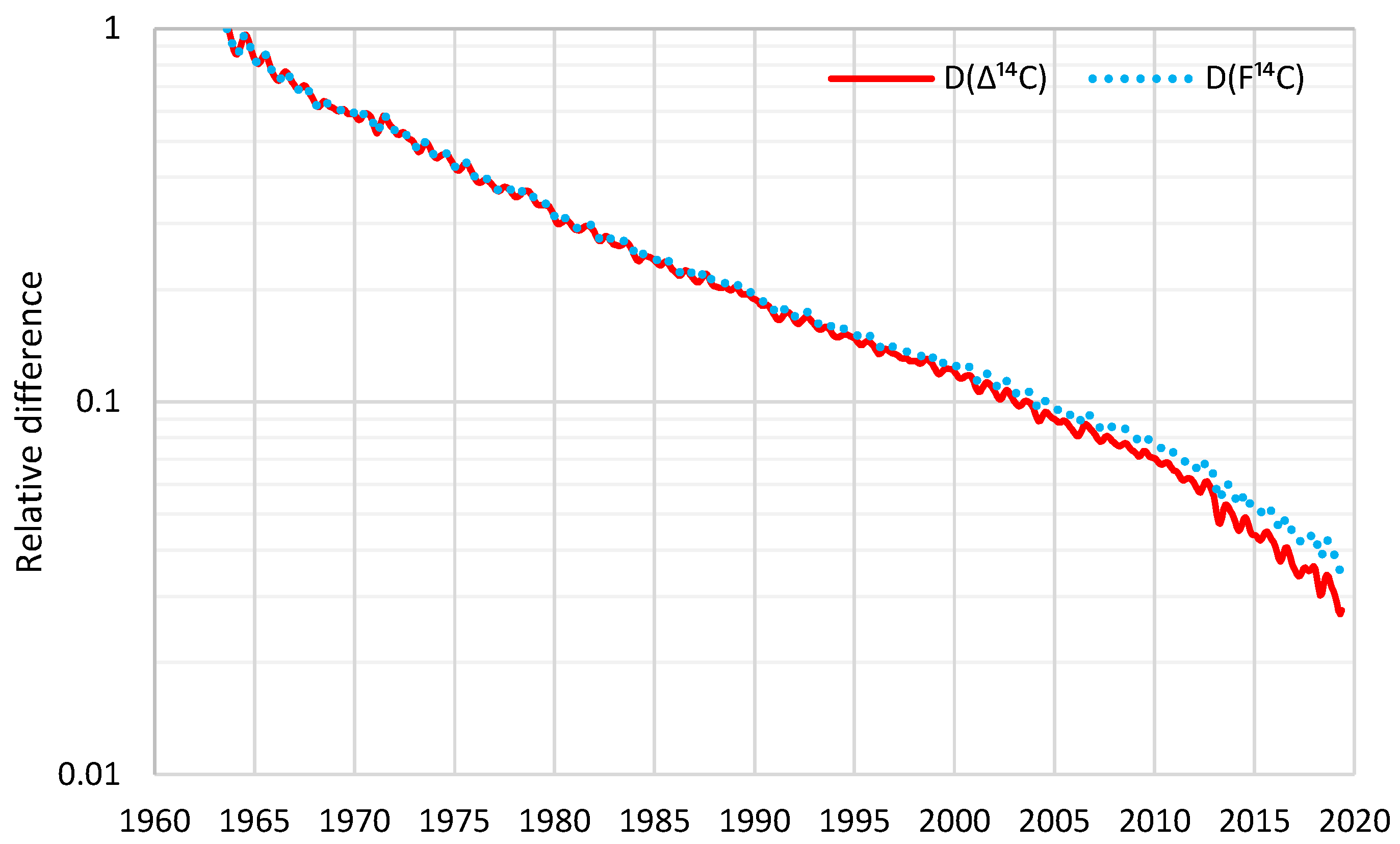
Eventually, we choose to analyze the series because Hua et al. [67] also provide a time series on a global basis for , which is depicted in Figure A2. Before we proceed to analyze this time series, it is useful to stress the following two quotations from their paper:
Decreases in atmospheric Δ14C from the mid-1960s to mid-1980s are mainly due to rapid exchange between the atmosphere and the biosphere and oceans […], while combustion of fossil fuels free of 14C is the main causal factor for the Δ14C decline since the late 1980s and early 1990s […]. Since the early and late 2000s, the atmospheric Δ14C values have been lower than those of the surface waters in the North and South Pacific Gyres, respectively, indicating the oceans might become a net 14C source (instead of a net 14C sink) of the atmosphere […]The last data points in our compiled monthly data at 2019.375 have respective F14C values of 1.0084 and 1.0195 for the NH and SH (see Supplementary Tables 2a–e), which are very close to the pre-bomb F14C value of slightly lower than 1. This indicates that clean-air F14C is likely to reach the pre-bomb value in the early 2020s […].
The first quotation guides us to focus our model and its fitting on the period 1965–1985, because (a) it most faithfully reflects the system dynamics sought, i.e., the exchange between the atmosphere and the biosphere and oceans, and (b) the IRF values are higher, as are their changes in time, and hence they are more appropriate for model fitting.
The second quotation expresses a blatant disagreement with IPCC claims of time lags reaching “several hundred thousand years”, given that the entire perturbation of 14C by bomb testing disappeared in about 55 years.
If we assume that the reservoir dynamics is linear, which is the simplest and most parsimonious case, then, according to corollary 2, the IRF will be exponential, i.e.,
where is the mean response time. Hence,
This model, with fitted 17.2 years, perfectly describes the data for the period 1965–1985, as seen in Figure A2. In addition, its extrapolation for the subsequent period (without changing the fitted parameters) agrees very well with the data. Hence, the simple linear reservoir is a good model for the system examined.
Figure A2.
Global time series, as provided by Hua et al. [67], and fitted linear reservoir model (Equation (A21)).
Figure A2.
Global time series, as provided by Hua et al. [67], and fitted linear reservoir model (Equation (A21)).
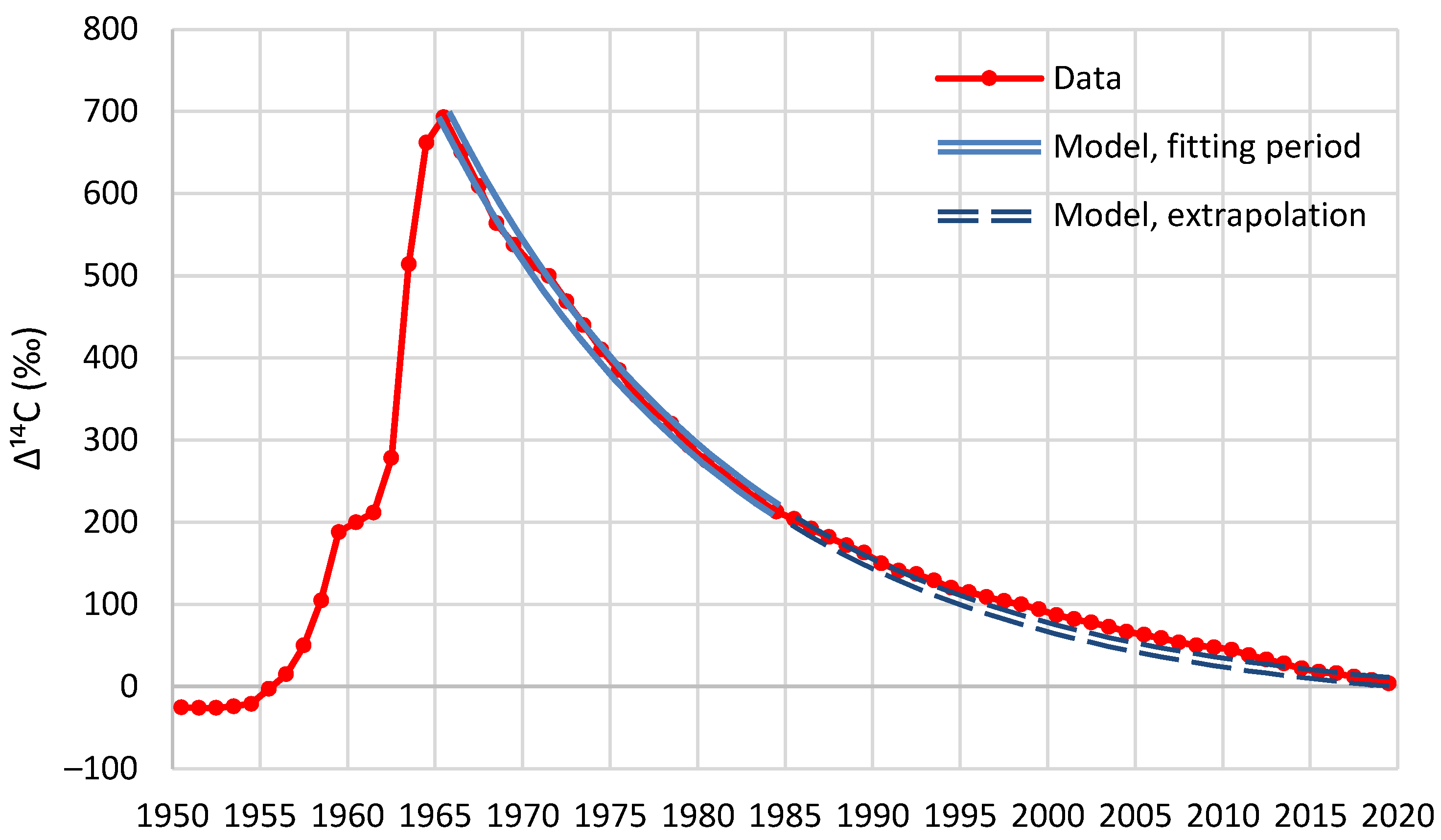
The two IRFs for the case, empirical (from data) and modeled (from Equation (A21) with = 17.2 years), are compared with two IRFs that refer to the total [CO2]. These are the IPCC model (Equation (50) with the coefficients shown in Table A1) and the linear reservoir model of the present study with years. The absolute incompatibility of the IPCC model with reality, as demonstrated through the Δ14C data (and the model fitted to them, which is in perfect agreement with the data) is obvious (Figure A3).
The relevant question is whether or not the Δ14C data and model are compatible with the linear reservoir model of the present study. The answer is affirmative, and the longer mean response time in the Δ14C case ( 17.2 years) compared to the total [CO2] case ( years) is expected. There are three very strong reasons for this increase in the response time of Δ14C:
- The absorption of the heavier isotope 14C is subject to a function known as fractionation, that is, isotope discrimination. In particular, photosynthesis, during the exchange of O2 and CO2, discriminates against the heavier isotopes, and, as a result, 14C remains in the atmosphere for longer periods.
- As already noted above, most of the 14C produced by nuclear weapons testing was injected into the stratosphere, and the transport from the stratosphere to the troposphere is a slow process, substantially increasing the time lags.
- While, by its definition, the IRF presupposes zero inflows after the impulse, in reality, there were additional 14C inflows due to anomalous neutron flux (corresponding to a systematic increase of 5–10% over the last 30 years, according to Harde and Salby [74]). The fact that these 14C inflows were not considered in the model led to an artificial increase in the actual response time.
The precise quantification of these factors is not easy and does not belong to the scope of this paper. Nonetheless, the 14C analysis offers an indirect validation of the RRR results by determining an upper bound of the response time, which the RRR model respects, while the IPCC model blatantly violates it.
Figure A3.
Comparison of two total [CO2] IRFs, i.e., (a) the IPCC model (Equation (50) with the coefficients shown in Table A1), (b) the results from the present study (a linear reservoir model with years), and two IRFs, i.e., (c) empirical (from data) and (d) modeled (from Equation (A21) with 17.2 years).
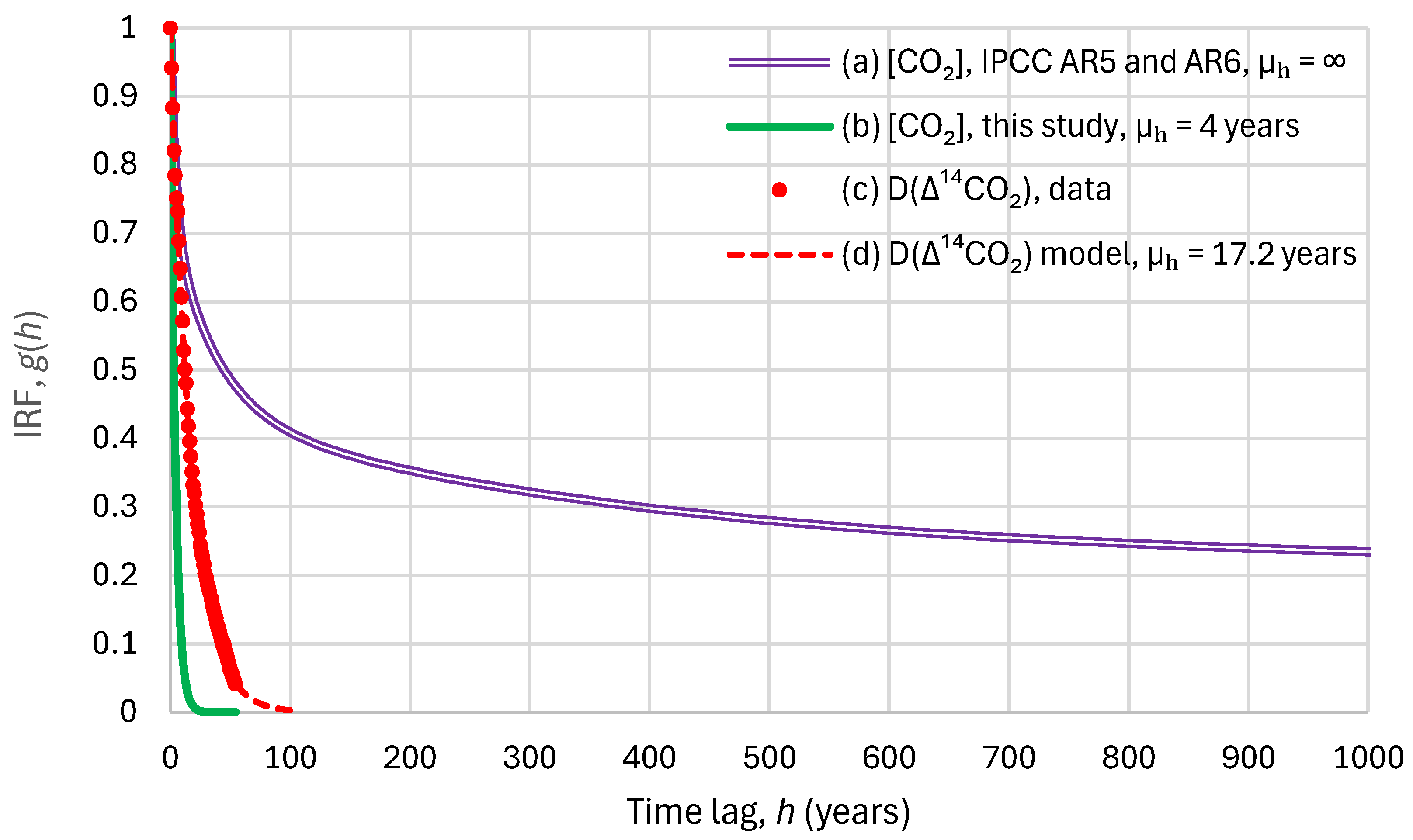
References
- Stendhal. The Life of Henry Brulard [Vie de Henry Brulard]; Sturrock, J., Translator; The New York Review of Books: New York, NY, USA, 1995; ISBN 978-1-681371-22-1. Available online: https://archive.org/details/stendhal-life-of-henry-brulard/ (accessed on 30 April 2024).
- Müller-Neuhof, B.; Betts, A.V.G.; Wilcox, G. Jawa, Northeastern Jordan: The first 14C dates for the early occupation phase. Z. Für Orient-Archäologie 2015, 8, 124–131. [Google Scholar]
- Fahlbusch, H. Early dams. Proc. ICE—Eng. Hist. Herit. 2009, 162, 13–18. [Google Scholar] [CrossRef]
- Makarewicz, C.A.; Finlayson, B. Constructing community in the Neolithic of southern Jordan: Quotidian practice in communal architecture. PLoS ONE 2018, 13, e0193712. [Google Scholar] [CrossRef]
- Bible, Genesis, 41. Available online: https://www.bible.com/el/bible/2503/GEN.41.GRCBRENT?parallel=392 (accessed on 30 April 2024).
- Bell, B. Climate and the History of Egypt: The Middle Kingdom. Am. J. Archaeol. 1975, 79, 223–269. [Google Scholar] [CrossRef]
- Said, R. The River Nile: Geology, Hydrology and Utilization; Pergamon Press: Oxford, UK, 1993. [Google Scholar]
- Hurst, H.E. Long term storage capacities of reservoirs. Trans. Am. Soc. Civ. Eng. 1951, 116, 776–808. [Google Scholar] [CrossRef]
- Mandelbrot, B.B.; Wallis, J.R. Noah, Joseph, and operational hydrology. Water Resour. Res. 1968, 4, 909–918. [Google Scholar] [CrossRef]
- Koutsoyiannis, D. Stochastics of Hydroclimatic Extremes—A Cool Look at Risk, 3rd ed.; Kallipos Open Academic Editions: Athens, Greece, 2023; p. 391. ISBN 978-618-85370-0-2. [Google Scholar] [CrossRef]
- Koutsoyiannis, D.; Onof, C.; Kundzewicz, Z.W.; Christofides, A. On Hens, Eggs, Temperatures and CO2: Causal Links in Earth’s Atmosphere. Sci 2023, 5, 35. [Google Scholar] [CrossRef]
- Peachey, B. Mitigating human enhanced water emission impacts on climate change. In Proceedings of the 2006 IEEE EIC Climate Change Conference, Ottawa, ON, Canada, 9–12 May 2006. [Google Scholar] [CrossRef]
- Sherwood, S.C.; Dixit, V.; Salomez, C. The global warming potential of near-surface emitted water vapor. Environ. Res. Lett. 2018, 13, 104006. [Google Scholar] [CrossRef]
- Li, X.; Peachey, B.; Maeda, N. Global warming and anthropogenic emissions of water vapor. Langmuir 2024, 40, 7701–7709. [Google Scholar] [CrossRef]
- Koutsoyiannis, D. Relative importance of carbon dioxide and water in the greenhouse effect: Does the tail wag the dog? Preprints 2024, 2024040309. [Google Scholar] [CrossRef]
- Klemeš, V. Watershed as semiinfinite storage reservoir. J. Irrig. Drain. Div. 1973, 99, 477–491. [Google Scholar] [CrossRef]
- Liu, Z.; Todini, E. Assessing the TOPKAPI non-linear reservoir cascade approximation by means of a characteristic lines solu-tion. Hydrol. Process. 2005, 19, 1983–2006. [Google Scholar] [CrossRef]
- Fenicia, F.; Savenije, H.H.G.; Matgen, P.; Pfister, L. Is the groundwater reservoir linear? Learning from data in hydrological modelling. Hydrol. Earth Syst. Sci. 2006, 10, 139–150. [Google Scholar] [CrossRef]
- Koutsoyiannis, D. Revisiting the global hydrological cycle: Is it intensifying? Hydrol. Earth Syst. Sci. 2020, 24, 3899–3932. [Google Scholar] [CrossRef]
- Nash, J.E.; Farrel, J.P. A graphical solution of the flood-routing equation for linear storage-discharge relation. Eos Trans. Am. Geophys. Union 1955, 36, 319–320. [Google Scholar]
- Langbein, W.B. Queuing theory and water storage. J. Hydraul. Div. 1958, 84, 1–24. [Google Scholar] [CrossRef]
- Nash, J.E. Systematic determination of unit hydrograph parameters. J. Geophys. Res. 1959, 64, 111–115. [Google Scholar] [CrossRef]
- Dooge, J. Linear Theory of Hydrologic Systems; No. 1468; Agricultural Research Service, US Department of Agriculture: Washington, DC, USA, 1973. Available online: https://books.google.com/books?id=iVgTfUhBi2gC (accessed on 20 April 2024).
- Klemeš, V. Probability distribution of outflow from a linear reservoir. J. Hydrol. 1974, 21, 305–314. [Google Scholar] [CrossRef]
- Klemeš, V.; Borůvka, L. Output from a cascade of discrete linear reservoirs with stochastic input. J. Hydrol. 1975, 27, 1–13. [Google Scholar] [CrossRef]
- Basha, H.A. Nonlinear reservoir routing: Particular analytical solution. J. Hydraul. Eng. 1994, 120, 624–632. [Google Scholar]
- Paik, K. Analytical derivation of reservoir routing and hydrological risk evaluation of detention basins. J. Hydrol. 2008, 352, 191–201. [Google Scholar] [CrossRef]
- Nematollahi, B.; Niazkar, M.; Talebbeydokhti, N. Analytical and numerical solutions to level pool routing equations for sim-plified shapes of inflow hydrographs. Iran. J. Sci. Technol. Trans. Civ. Eng. 2022, 46, 1–15. [Google Scholar] [CrossRef]
- Basha, H.A. Routing equations for detention reservoirs. J. Hydraul. Eng. 1995, 121, 885–888. [Google Scholar] [CrossRef]
- Berry, E.X. Human CO2 emissions have little effect on atmospheric CO2. Int. J. Atmos. Ocean. Sci. 2019, 3, 13–26. [Google Scholar]
- IPCC. Climate Change 2013: The Physical Science Basis. Contribution of Working Group I to the Fifth Assessment Report of the Intergovernmental Panel on Climate Change; Stocker, T.F., Qin, D., Plattner, G.-K., Tignor, M., Allen, S.K., Boschung, J., Nauels, A., Xia, Y., Bex, V., Midgley, P.M., Eds.; Cambridge University Press: Cambridge, UK; New York, NY, USA, 2013. [Google Scholar]
- IPCC. Climate Change 2021: The Physical Science Basis. Contribution of Working Group I to the Sixth Assessment Report of the Intergovernmental Panel on Climate Change; Masson-Delmotte, V., Zhai, P., Pirani, A., Connors, S.L., Péan, C., Berger, S., Caud, N., Chen, Y., Goldfarb, L., Gomis, M.I., et al., Eds.; Cambridge University Press: Cambridge, UK; New York, NY, USA, 2021; p. 2391. [Google Scholar] [CrossRef]
- Koutsoyiannis, D.; Onof, C.; Christofides, A.; Kundzewicz, Z.W. Revisiting causality using stochastics: 1. Theory. Proc. R. Soc. A 2022, 478, 20210835. [Google Scholar] [CrossRef]
- Koutsoyiannis, D.; Onof, C.; Christofides, A.; Kundzewicz, Z.W. Revisiting causality using stochastics: 2. Applications. Proc. R. Soc. A 2022, 478, 20210836. [Google Scholar] [CrossRef]
- Koutsoyiannis, D. Stochastic assessment of temperature—CO2 causal relationship in climate from the Phanerozoic through modern times. Math. Biosci. Eng. 2024, 21, 6560–6602. [Google Scholar] [CrossRef]
- Salby, M.L. Physics of the Atmosphere and Climate; Cambridge University Press: New York, NY, USA, 2012. [Google Scholar]
- Humlum, O.; Stordahl, K.; Solheim, J.E. The phase relation between atmospheric carbon dioxide and global temperature. Glob. Planet. Chang. 2013, 100, 51–69. [Google Scholar] [CrossRef]
- Harde, H. Scrutinizing the carbon cycle and CO2 residence time in the atmosphere. Glob. Planet. Chang. 2017, 152, 19–26. [Google Scholar] [CrossRef]
- Harde, H. What humans contribute to atmospheric CO2: Comparison of carbon cycle models with observations. Earth Sci. 2019, 8, 139–159. [Google Scholar]
- Poyet, P. The Rational Climate e-Book, 2nd ed.; ResearchGate; ISBN 978-99957-1-929-62022. Available online: https://www.researchgate.net/publication/347150306 (accessed on 30 April 2024).
- Stallinga, P. Residence time vs. adjustment time of carbon dioxide in the atmosphere. Entropy 2023, 25, 384. [Google Scholar] [CrossRef] [PubMed]
- Joos, F.; Roth, R.; Fuglestvedt, J.S.; Peters, G.P.; Enting, I.G.; von Bloh, W.; Brovkin, V.; Burke, E.J.; Eby, M.; Edwards, N.R.; et al. Carbon dioxide and climate impulse response functions for the computation of greenhouse gas metrics: A multi-model analysis. Atmos. Chem. Phys. 2013, 13, 2793–2825. [Google Scholar] [CrossRef]
- Joos, F.; Bruno, M.; Fink, R.; Siegenthaler, U.; Stocker, T.F.; Le Quere, C.; Sarmiento, J.L. An efficient and accurate representation of complex oceanic and biospheric models of anthropogenic carbon uptake. Tellus B 1996, 48, 397–417. [Google Scholar] [CrossRef]
- Archer, D.; Brovkin, V. The millennial atmospheric lifetime of anthropogenic CO2. Clim. Chang. 2008, 90, 283–297. [Google Scholar] [CrossRef]
- Archer, D.; Eby, M.; Brovkin, V.; Ridgwell, A.; Cao, L.; Mikolajewicz, U.; Caldeira, K.; Matsumoto, K.; Munhoven, G.; Mon-tenegro, A.; et al. Atmospheric lifetime of fossil fuel carbon dioxide. Annu. Rev. Earth Planet. Sci. 2009, 37, 117–134. [Google Scholar] [CrossRef]
- MIT Climate Portal Writing Team Featuring Guest Expert Ed Boyle, How Do We Know How Long Carbon Dioxide Remains in the Atmosphere? MIT Climate Portal. 2023. Available online: https://climate.mit.edu/ask-mit/how-do-we-know-how-long-carbon-dioxide-remains-atmosphere (accessed on 30 April 2024).
- Buis, A. The Atmosphere: Getting a Handle on Carbon Dioxide, NASA’s Jet Propulsion Laboratory. 2019. Available online: https://science.nasa.gov/earth/climate-change/greenhouse-gases/the-atmosphere-getting-a-handle-on-carbon-dioxide/ (accessed on 30 April 2024).
- Berry, E. Why Climate Change Is a Fraud. Available online: https://edberry.com/why-climate-change-is-a-fraud/ (accessed on 30 April 2024).
- Myhre, G.; Shindell, D.; Bréon, F.-M.; Collins, W.; Fuglestvedt, J.; Huang, J.; Koch, D.; Lamarque, J.-F.; Lee, D.; Mendoza, B.; et al. Anthropogenic and natural radiative forcing supplementary material. In Climate Change 2013: The Physical Science Basis. Contribution of Working Group I to the Fifth Assessment Report of the Intergovernmental Panel on Climate Change; Stocker, T.F., Qin, D., Plattner, G.-K., Tignor, M., Allen, S.K., Boschung, J., Nauels, A., Xia, Y., Bex, V., Midgley, P.M., Eds.; Cambridge University Press: Cambridge, UK; New York, NY, USA, 2013; p. 1535. Available online: https://www.ipcc.ch/report/ar5/wg1/chapter-8sm-anthropogenic-and-natural-radiative-forcing-supplementary-material/ (accessed on 30 April 2024).
- Strassmann, K.M.; Joos, F. The Bern Simple Climate Model (BernSCM) v1.0: An extensible and fully documented open-source re-implementation of the Bern reduced-form model for global carbon cycle–climate simulations. Geosci. Model Dev. 2018, 11, 1887–1908. [Google Scholar] [CrossRef]
- Luo, X.; Xia, T.; Huang, J.; Xiong, D.; Ridoutt, B. Radiative forcing climate footprints in the agricultural sector: Comparison of models from the IPCC 5th and 6th Assessment Reports. Farming Syst. 2023, 1, 100057. [Google Scholar] [CrossRef]
- Keeling, C.D.; Piper, S.C.; Whorf, T.P.; Keeling, R.F. Evolution of natural and anthropogenic fluxes of atmospheric CO2 from 1957 to 2003. Tellus B Chem. Phys. Meteorol. 2011, 63, 1–22. [Google Scholar] [CrossRef]
- Scripps CO2 Program, Sampling Station Records. Available online: https://scrippsco2.ucsd.edu/data/atmospheric_co2/sampling_stations.html (accessed on 30 April 2024).
- Keeling, C.D.; Piper, S.C.; Bacastow, R.B.; Wahlen, M.; Whorf, T.P.; Heimann, M.; Meijer, H.A. Exchanges of Atmospheric CO2 and 13CO2 with the Terrestrial Biosphere and Oceans from 1978 to 2000. I. Global Aspects; SIO Reference Series, No. 01-06; Scripps Institution of Oceanography: San Diego, CA, USA, 2001; p. 88. [Google Scholar]
- Keeling, C.D.; Piper, S.C.; Bacastow, R.B.; Wahlen, M.; Whorf, T.P.; Heimann, M.; Meijer, H.A. Atmospheric CO2 and 13CO2 exchange with the terrestrial biosphere and oceans from 1978 to 2000: Observations and carbon cycle implications. In A History of Atmospheric CO2 and Its Effects on Plants; Ehleringer, J.R., Cerling, T.E., Dearing, M.D., Eds.; Springer: New York, NY, USA, 2005; pp. 83–113. [Google Scholar]
- Ritchie, H.; Roser, M. CO2 Emissions. OurWorldInData.org. 2020. Available online: https://ourworldindata.org/co2-emissions (accessed on 30 April 2024).
- Global Carbon Budget (2023)—With Major Processing by Our World in Data. “Annual CO2 Emissions—GCB” [Dataset]. Global Carbon Project, “Global Carbon Budget” [Original Data]. Available online: https://ourworldindata.org/co2-and-greenhouse-gas-emissions (accessed on 30 April 2024).
- International Energy Agency. CO2 Emissions in 2023. 2024. Available online: https://iea.blob.core.windows.net/assets/33e2badc-b839-4c18-84ce-f6387b3c008f/CO2Emissionsin2023.pdf (accessed on 30 April 2024).
- Koutsoyiannis, D.; Kundzewicz, Z.W. Atmospheric temperature and CO2: Hen-or-egg causality? Sci 2020, 2, 83. [Google Scholar] [CrossRef]
- Patel, K.F.; Bond-Lamberty, B.; Jian, J.L.; Morris, K.A.; McKever, S.A.; Norris, C.G.; Zheng, J.; Bailey, V.L. Carbon flux estimates are sensitive to data source: A comparison of field and lab temperature sensitivity data. Environ. Res. Lett. 2022, 17, 113003. [Google Scholar] [CrossRef]
- Robinson, C. Microbial respiration, the engine of ocean deoxygenation. Front. Mar. Sci. 2019, 5, 533. [Google Scholar] [CrossRef]
- Klemeš, V. Operational testing of hydrological simulation models. Hydrol. Sci. J. 1986, 31, 13–24. [Google Scholar] [CrossRef]
- Granger, C.W. Investigating causal relations by econometric models and cross-spectral methods. Econometrica 1969, 37, 424–438. [Google Scholar] [CrossRef]
- Koutsoyiannis, D.; Vournas, C. Revisiting the greenhouse effect—A hydrological perspective. Hydrol. Sci. J. 2024, 69, 151–164. [Google Scholar] [CrossRef]
- Koutsoyiannis, D. Net isotopic signature of atmospheric CO2 sources and sinks: No change since the Little Ice Age. Sci 2024, 6, 17. [Google Scholar] [CrossRef]
- Graven, H.; Keeling, R.F.; Rogelj, J. Changes to carbon isotopes in atmospheric CO2 over the industrial era and into the future. Glob. Biogeochem. Cycles 2020, 34, e2019GB006170. [Google Scholar] [CrossRef] [PubMed]
- Hua, Q.; Turnbull, J.C.; Santos, G.M.; Rakowski, A.Z.; Ancapichún, S.; De Pol-Holz, R.; Hammer, S.; Lehman, S.J.; Levin, I.; Miller, J.B.; et al. Atmospheric radiocarbon for the period 1950–2019. Radiocarbon 2022, 64, 723–745. [Google Scholar] [CrossRef]
- Kondev, F.G.; Wang, M.; Huang, W.J.; Naimi, S.; Audi, G. The NUBASE2020 evaluation of nuclear physics properties. Chin. Phys. C 2021, 45, 030001. [Google Scholar] [CrossRef]
- Starr, C. Atmospheric CO2 residence time and the carbon cycle. Energy 1993, 18, 1297–1310. [Google Scholar] [CrossRef]
- Berry, E.X. The impact of human CO2 on atmospheric CO2. Sci. Clim. Chang. 2021, 1, 1–46. [Google Scholar]
- Berry, E.X. Nature Controls the CO2 Increase. Sci. Clim. Chang. 2023, 3, 68–91. [Google Scholar]
- Salby, M.; Harde, H. Control of atmospheric CO2-Part I: Relation of carbon 14 to the removal of CO2. Sci. Clim. Chang. 2021, 1, 177–195. [Google Scholar]
- Salby, M.; Harde, H. Control of atmospheric CO2- Part II: Influence of Tropical Warming. Sci. Clim. Chang. 2021, 1, 197–213. [Google Scholar]
- Harde, H.; Salby, M. What controls the atmospheric CO2 level. Sci. Clim. Chang. 2021, 1, 54–69. [Google Scholar]
- Andrews, D.E. Correcting an error in some interpretations of atmospheric 14C data. Earth Sci. 2020, 9, 126–129. [Google Scholar]
- Reimer, P.J.; Brown, T.A.; Reimer, R.W. Discussion: Reporting and calibration of postbomb 14C data. Radiocarbon 2004, 46, 1299–1304. [Google Scholar]
- Currie, L.A.; Stafford, T.W.; Sheffield, A.E.; Klouda, G.A.; Wise, S.A.; Fletcher, R.A.; Donahue, D.J.; Jull, A.T.; Linick, T.W. Microchemical and molecular dating. Radiocarbon 1989, 31, 448–463. [Google Scholar]
- Stenström, K.; Skog, G.; Georgiadou, E.; Genberg, J.; Mellström, A. A Guide to Radiocarbon Units and Calculations. Lund University, Department of Physics, Internal Report LUNFD6(NFFR-3111)/1-17/(2011). 2011. Available online: https://portal.research.lu.se/files/5555659/2173661.pdf (accessed on 30 July 2024).
Figure 1.
Comparison of the exact (lines) and approximate (dots) solutions for the indicated cases and for constant inflow. The exact solutions are derived from (left) Equation (19) (superlinear reservoir, ) and (right) Equation (20) (sublinear reservoir, ). The approximate solutions are derived from Equation (11).
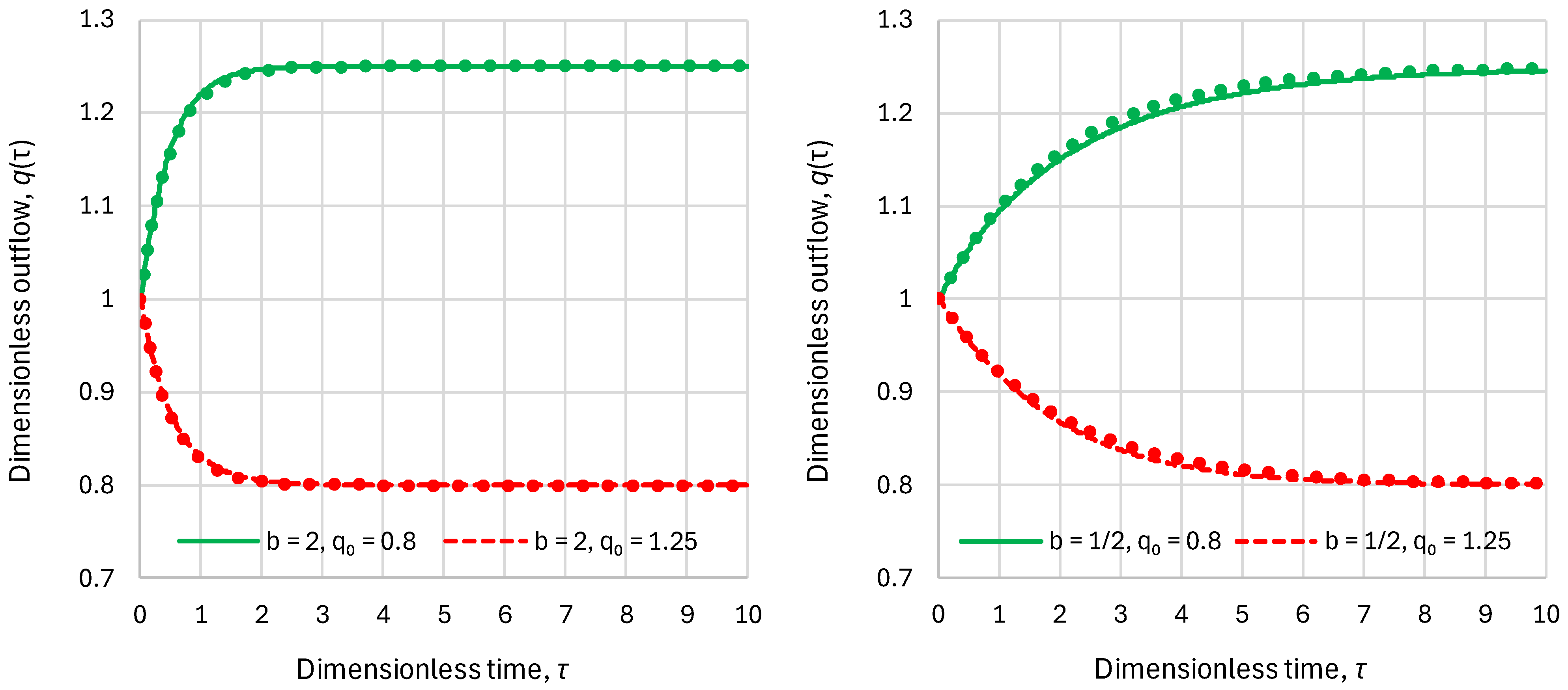
Figure 2.
Comparison of the exact (lines) and approximate (points) solutions for and (left) and (right) and for the indicated cases. In the case of the constant inflow (), the exact solution is derived from Equation (19) and the approximate solution from Equation (11). The cases of increasing and decreasing flow correspond to and , respectively, and the exact curves were determined by numerical integration, while the approximate solutions were determined by Equation (15).

Figure 3.
Probability plots of the distribution function of the dimensionless residence time for the indicated cases and constant inflow. The exact distributions (lines) are determined by numerical integration of Equations (29)–(31) and are compared to approximate analytical solutions (dots) determined by Equation (34).
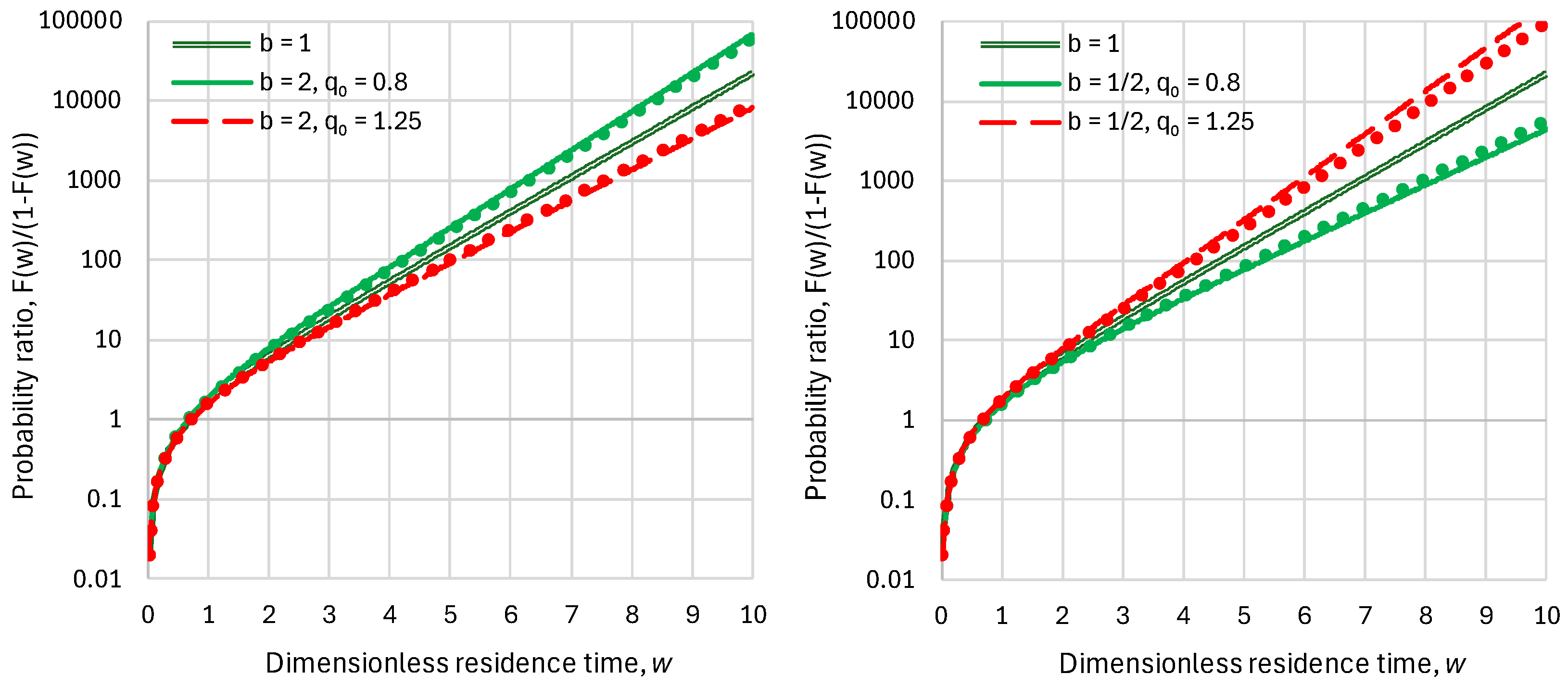
Figure 4.
Comparison of the mean dimensionless residence time from exact benchmark solutions (Equations (30) and (31) with numerical integration to find ) and approximations 1 and 2 (Equations (39) and (41), respectively).
Figure 4.
Comparison of the mean dimensionless residence time from exact benchmark solutions (Equations (30) and (31) with numerical integration to find ) and approximations 1 and 2 (Equations (39) and (41), respectively).
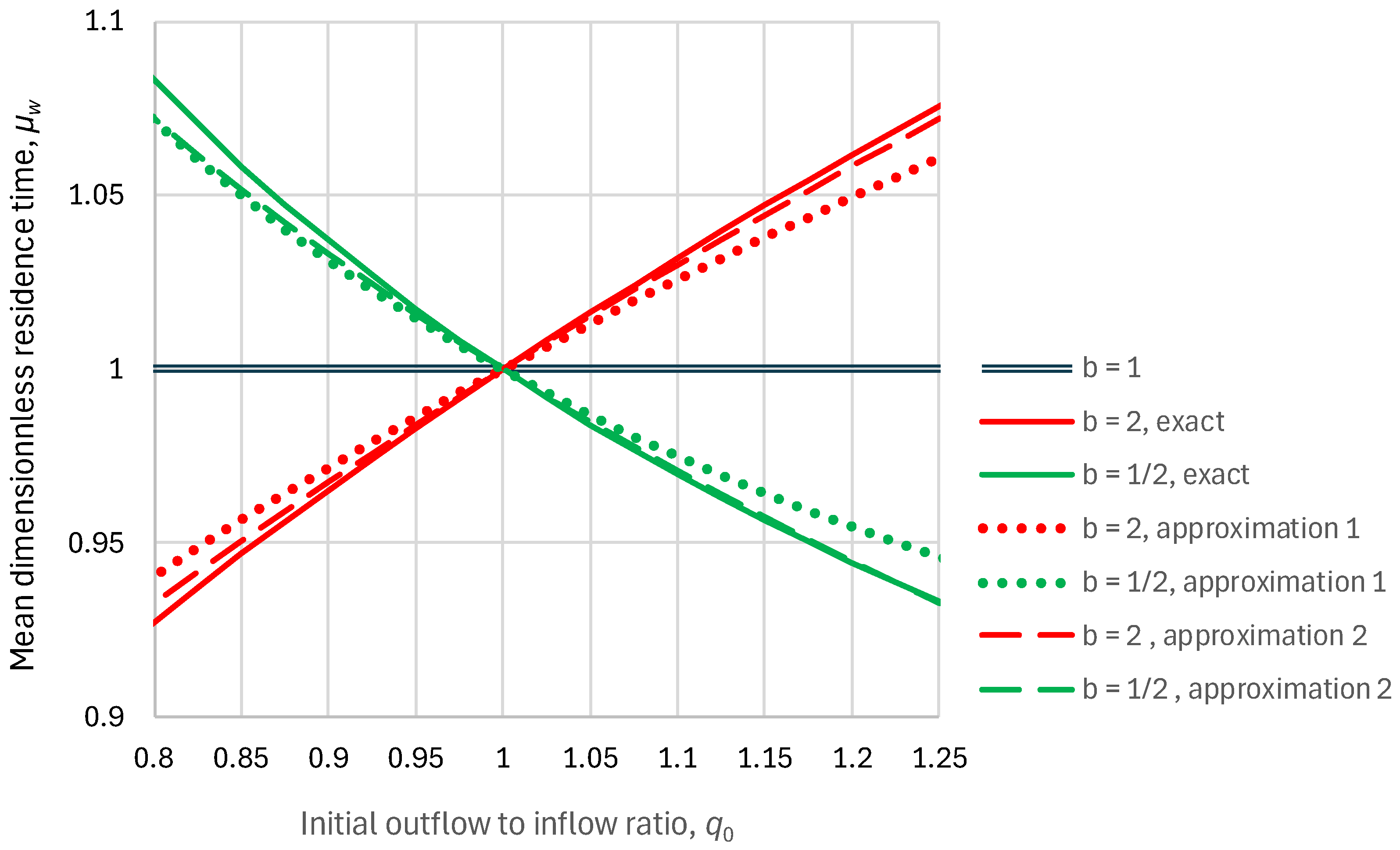
Figure 5.
Comparison of the mean dimensionless residence time for the indicated cases. Continuous lines for constant inflow () were obtained from Equations (30) and (31) (with numerical integration to find ), and those for increasing () and decreasing () inflow were found by numerical integration of the exact differential equations (considering a finite upper limit of integration, determined such as to avoid numerical instabilities). Beside each exact curve, that of approximation 2 (Equation (41)) is also plotted as a dashed line.
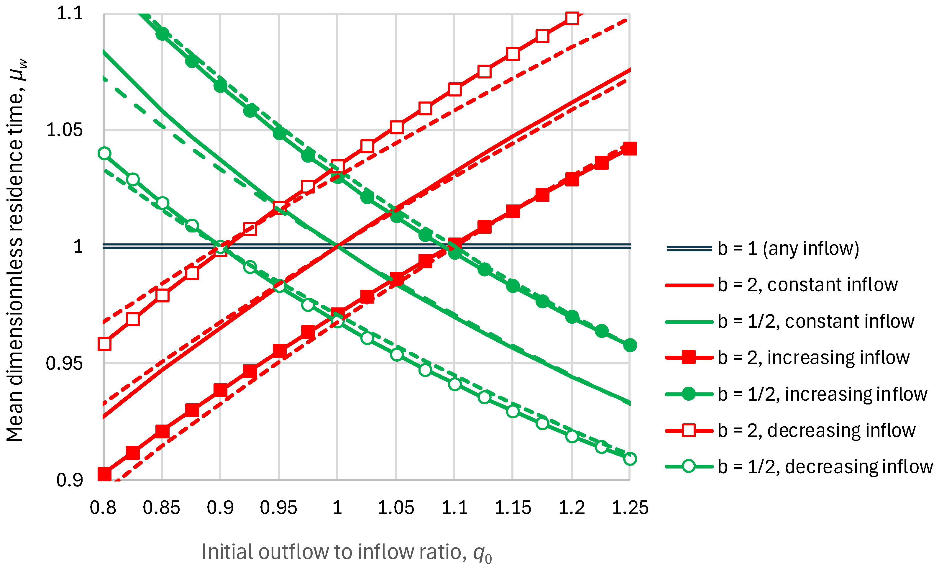
Figure 6.
Comparison of characteristic dimensionless time lags for the indicated cases. Mean and median residence times are determined from approximation 2 (Equation (41)). Response times are determined from the exact solution (Equation (44)). The mean response time in the bottom left graph () is infinite.
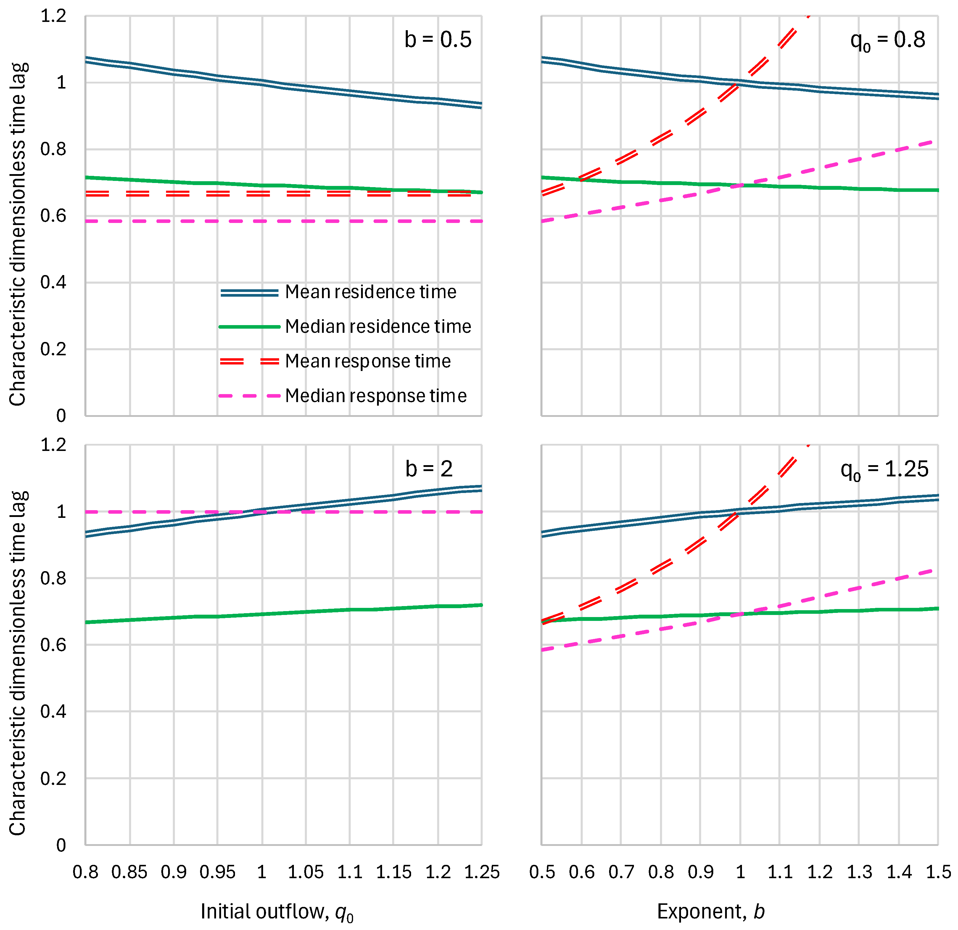
Figure 7.
Dimensionless outflow for zero inflow in the indicated cases, representing an impulse response function, with comparison of exact solutions (Equation (17)) and approximate ones (Equation (14)). In the right panel (sublinear reservoir, ), according to the exact solution, the reservoir empties at time , while according to the linear reservoir approximation, the emptying time is ; beyond emptying time, the outflow is zero.
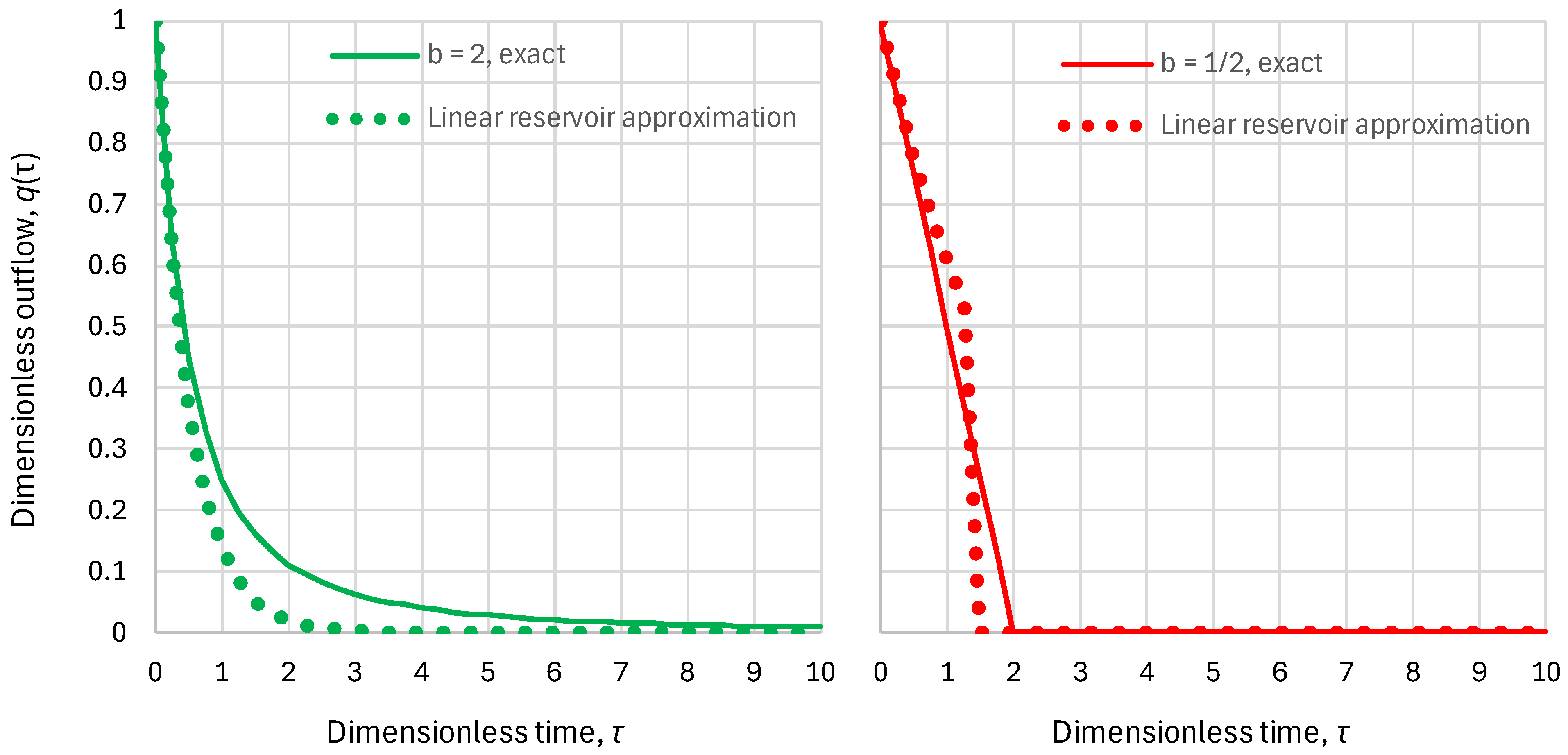
Figure 8.
Probability plots of the distribution function of dimensionless residence time for the indicated cases and zero inflow, with comparison of the exact solution (Equation (38)) with the linear reservoir approximation (Equation (14), which, combined with Equation (27), yields ).
Figure 8.
Probability plots of the distribution function of dimensionless residence time for the indicated cases and zero inflow, with comparison of the exact solution (Equation (38)) with the linear reservoir approximation (Equation (14), which, combined with Equation (27), yields ).
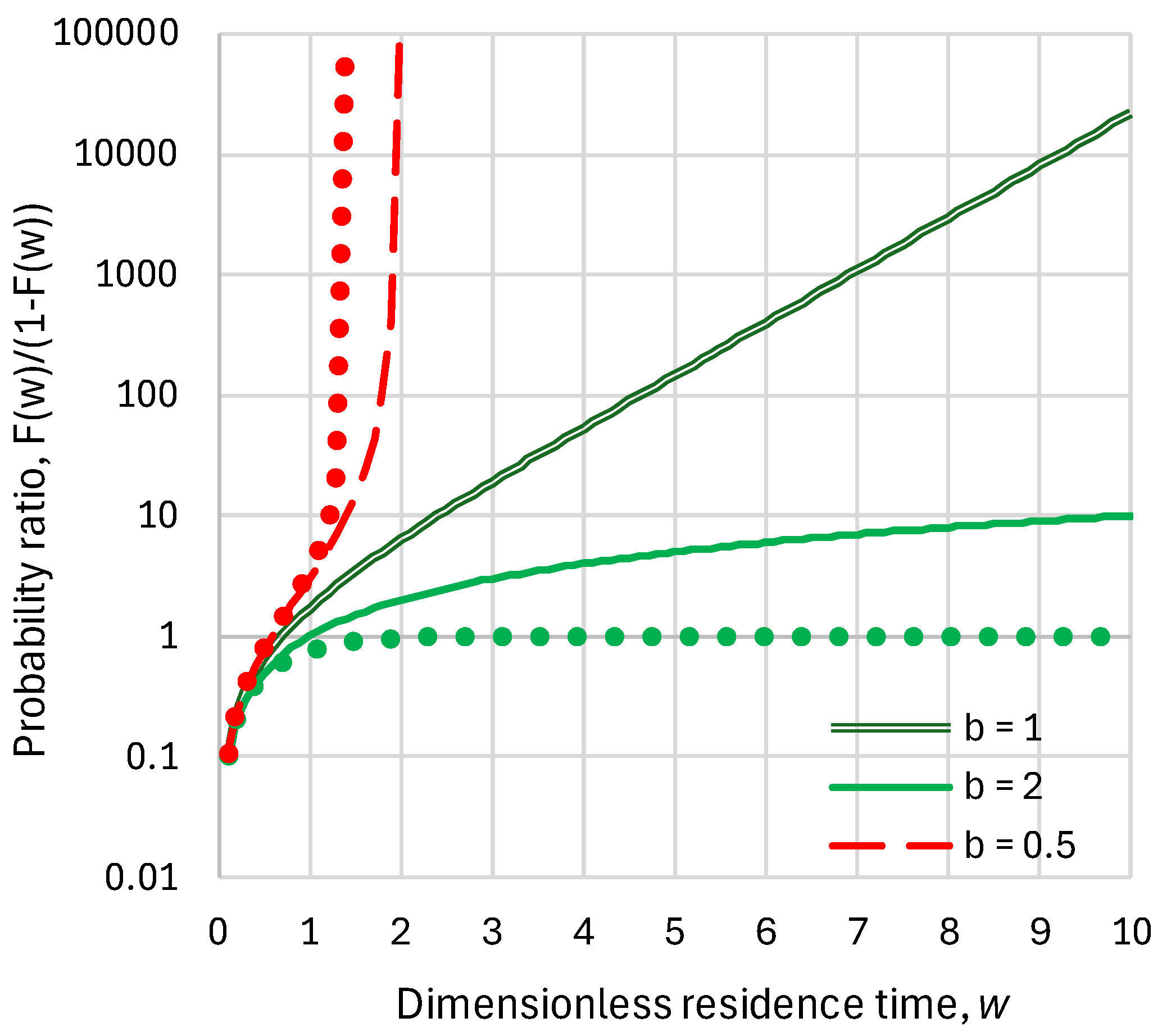
Figure 9.
Annual carbon balance in the Earth’s atmosphere, in ppm CO2/year, based on the IPCC estimates [32] (Figure 5.12). The balance of 2.4 ppm CO2/year is the annual CO2 accumulation in the atmosphere. The total of the modern natural additions (64.2 + 36.5 − (52.2 + 25.6)) = 22.9 ppm is 4.4 times larger than the human emissions (4.4 + 0.8 = 5.2 ppm). (Adapted from [11]).
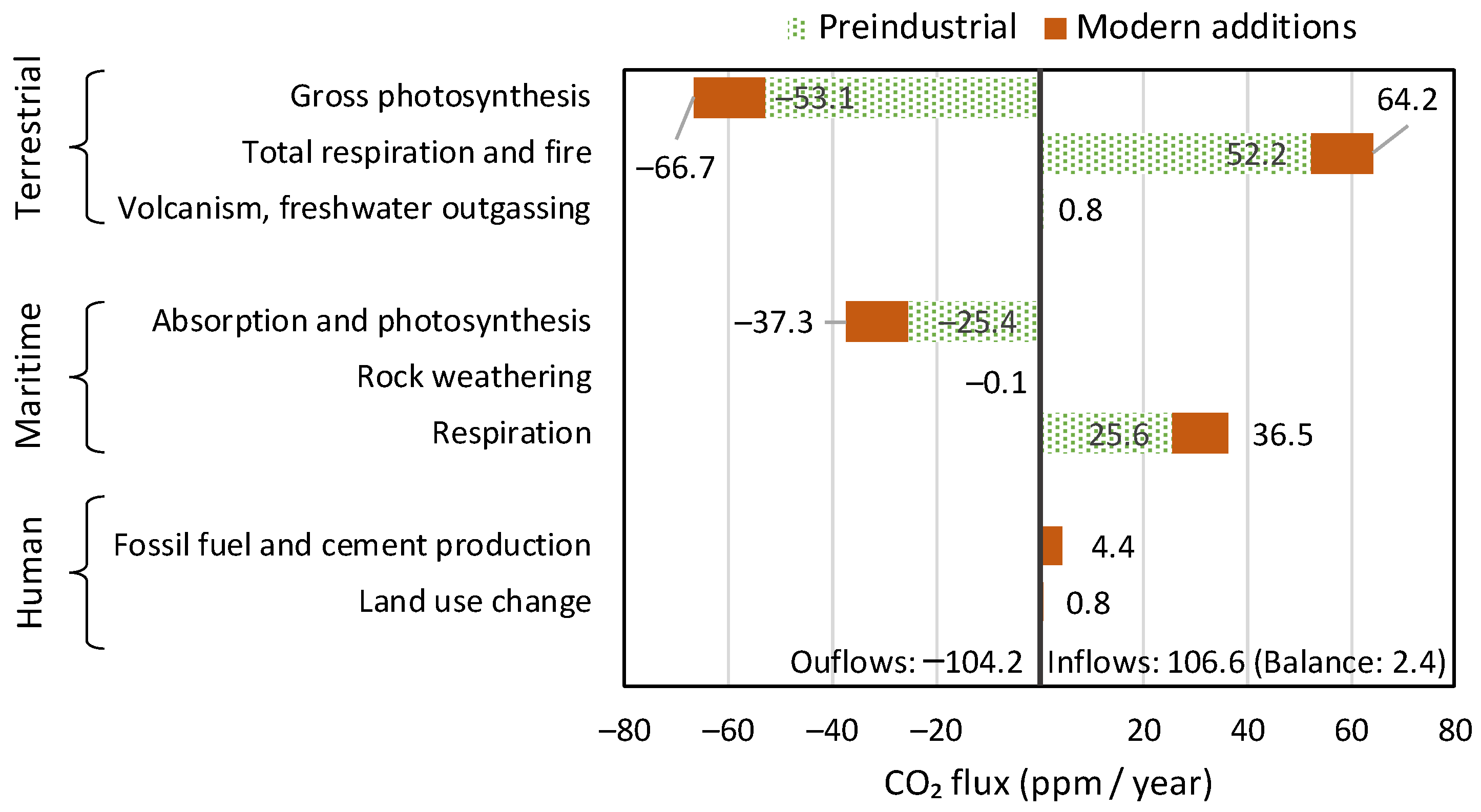
Figure 10.
Atmospheric carbon dioxide inflows and outflows as a function of carbon dioxide concentration. Large circles correspond to IPCC estimates for 1750 and the recent decade (assigned to 2017), and the line joining them is a power law with slope . The other circles have been determined using the method, as in Koutsoyiannis et al. [11], and the triangles by the same method but using 30% higher values of . A power law for output (not drawn in the graph) has a slope of 0.77.
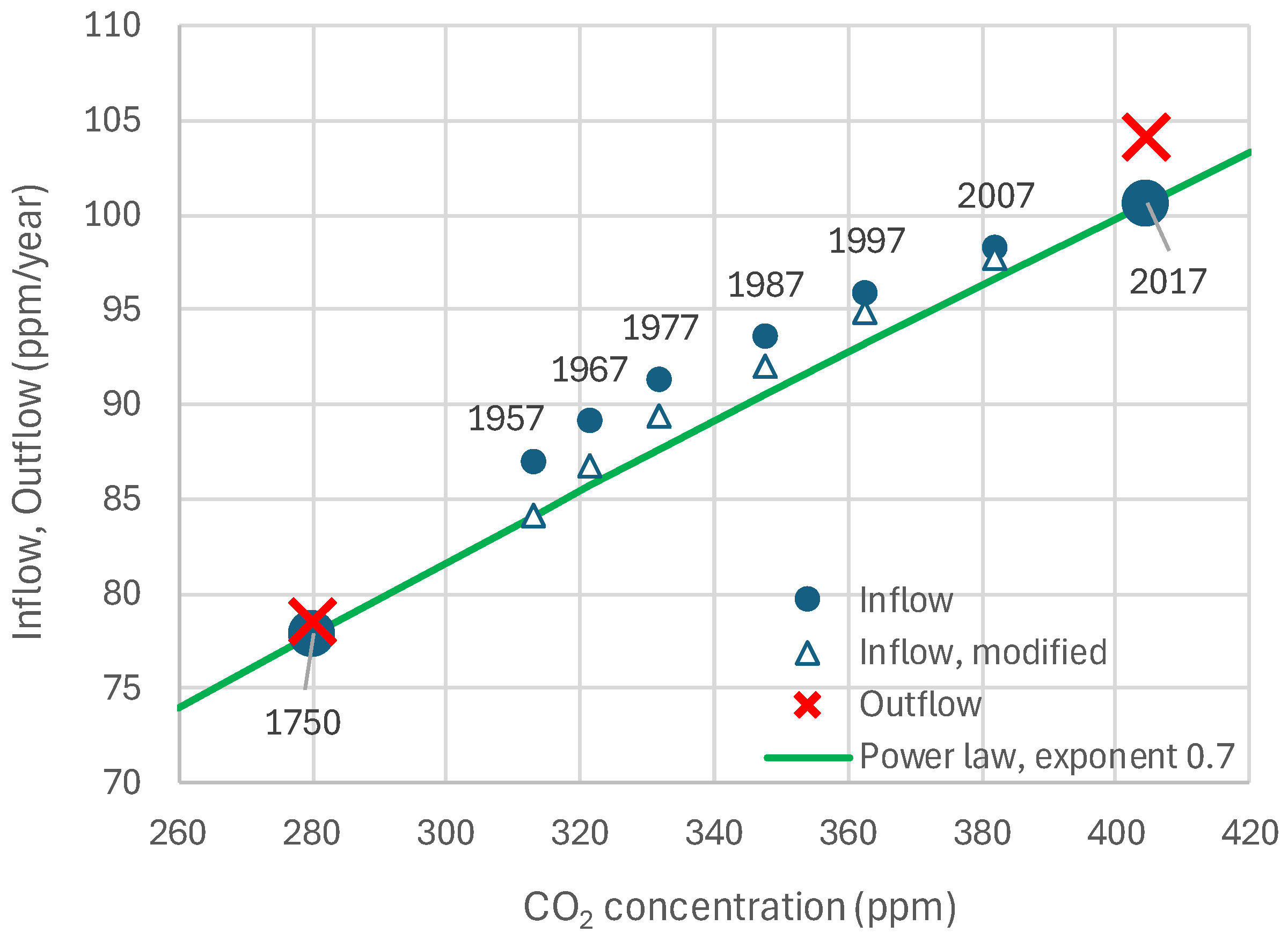
Figure 11.
Optimized values of (the exponent of the power law of inflow) as a function of the values of (the exponent of the power law of outflow). The optimization was made by fixing to a specified value and letting all other parameters free.
Figure 11.
Optimized values of (the exponent of the power law of inflow) as a function of the values of (the exponent of the power law of outflow). The optimization was made by fixing to a specified value and letting all other parameters free.
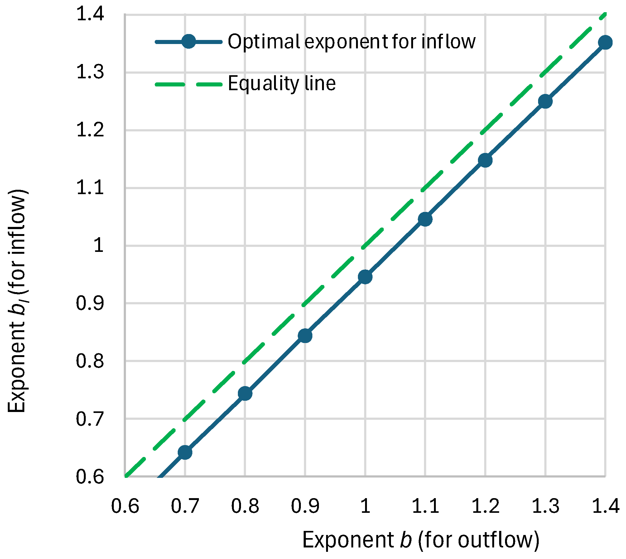
Figure 12.
Achieved values of the indicated explained variances, after maximizing their sum by fixing to a specified value and letting all other parameters free.
Figure 12.
Achieved values of the indicated explained variances, after maximizing their sum by fixing to a specified value and letting all other parameters free.
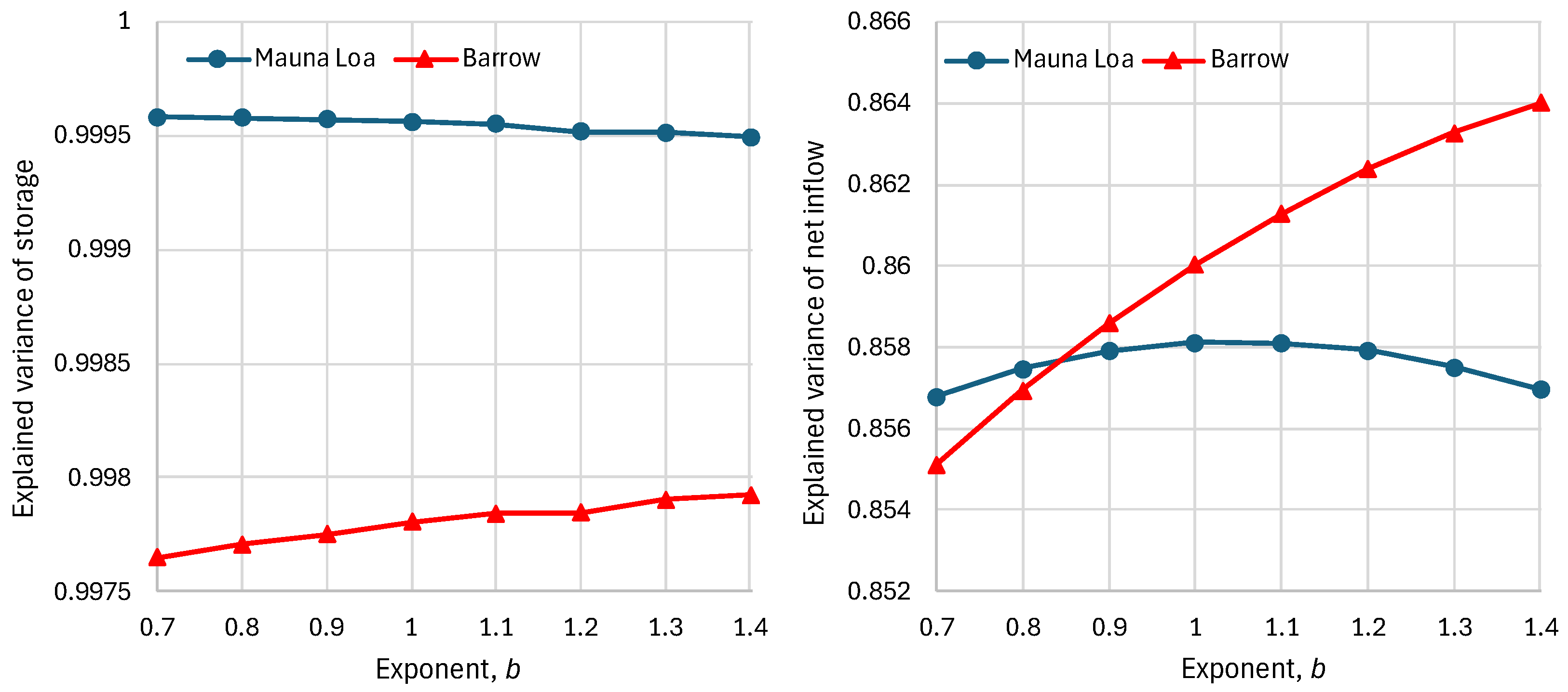
Figure 13.
Comparison of observed and simulated storage, , for (upper) Mauna Loa and (lower) Barrow. The insets show the seasonal variation of the characteristic times .
Figure 13.
Comparison of observed and simulated storage, , for (upper) Mauna Loa and (lower) Barrow. The insets show the seasonal variation of the characteristic times .
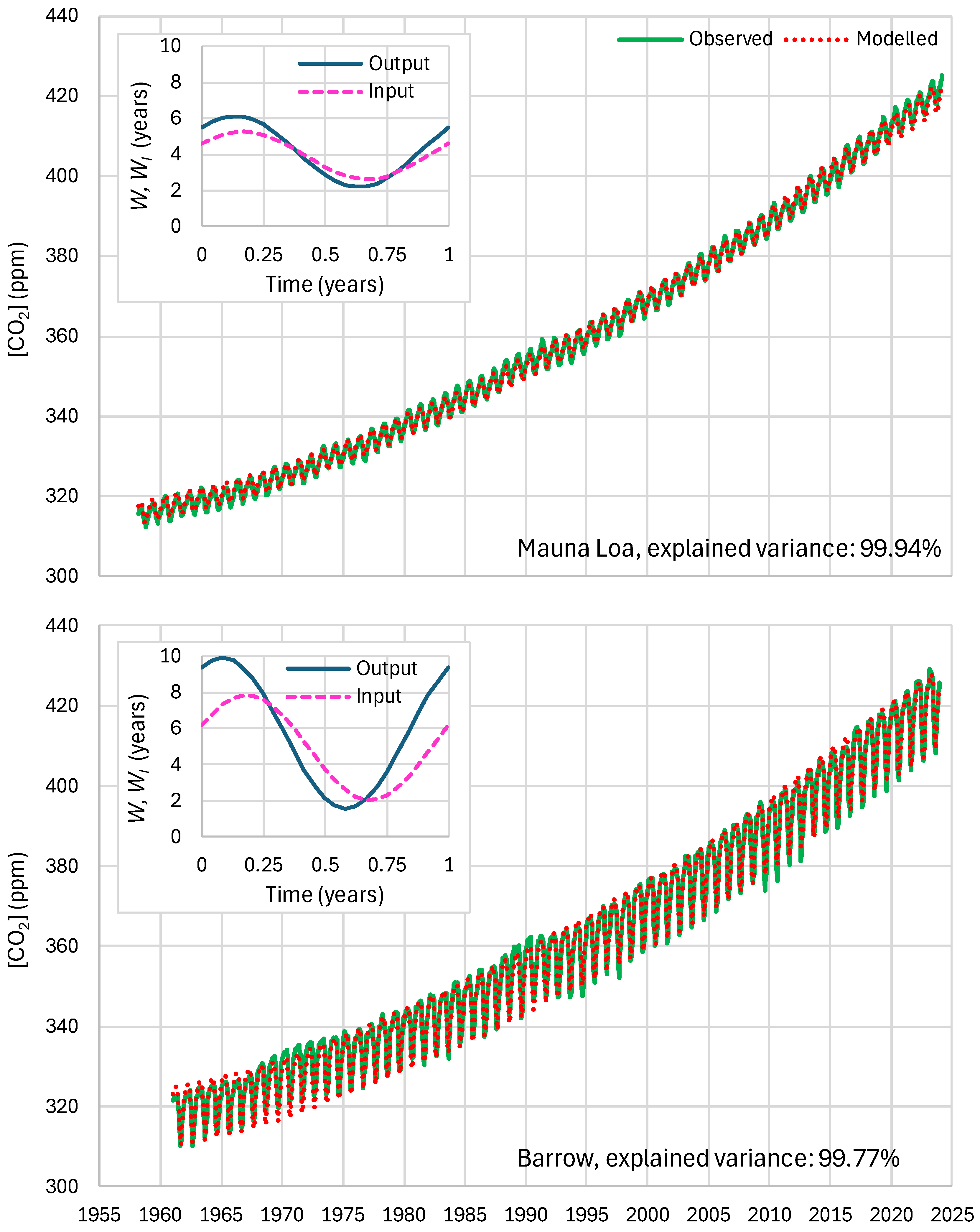
Figure 14.
Simulated inflows and outflows for (upper) Mauna Loa and (lower) Barrow.
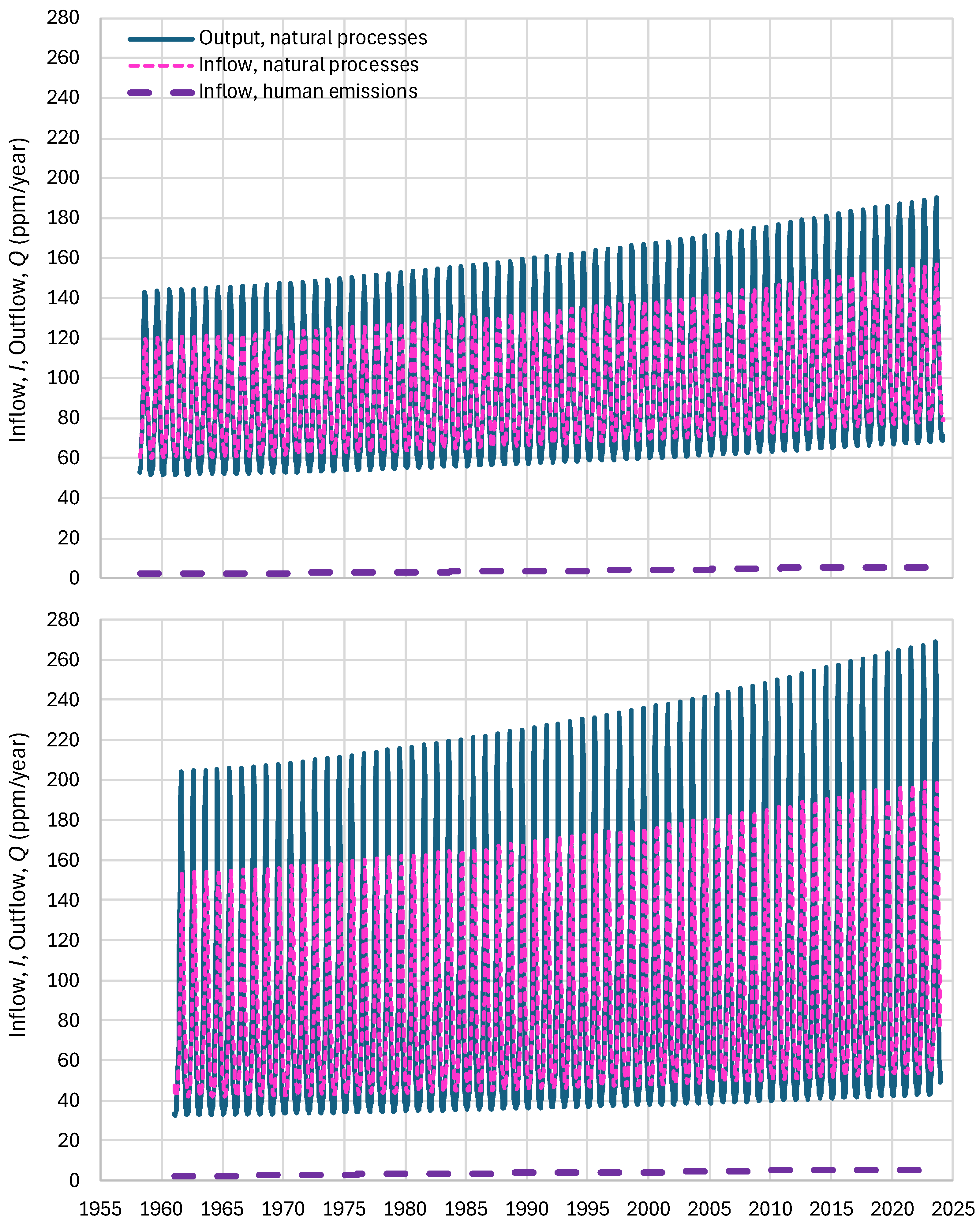
Figure 15.
Comparison of observed and simulated net inflows for (upper) Mauna Loa and (lower) Barrow.
Figure 15.
Comparison of observed and simulated net inflows for (upper) Mauna Loa and (lower) Barrow.
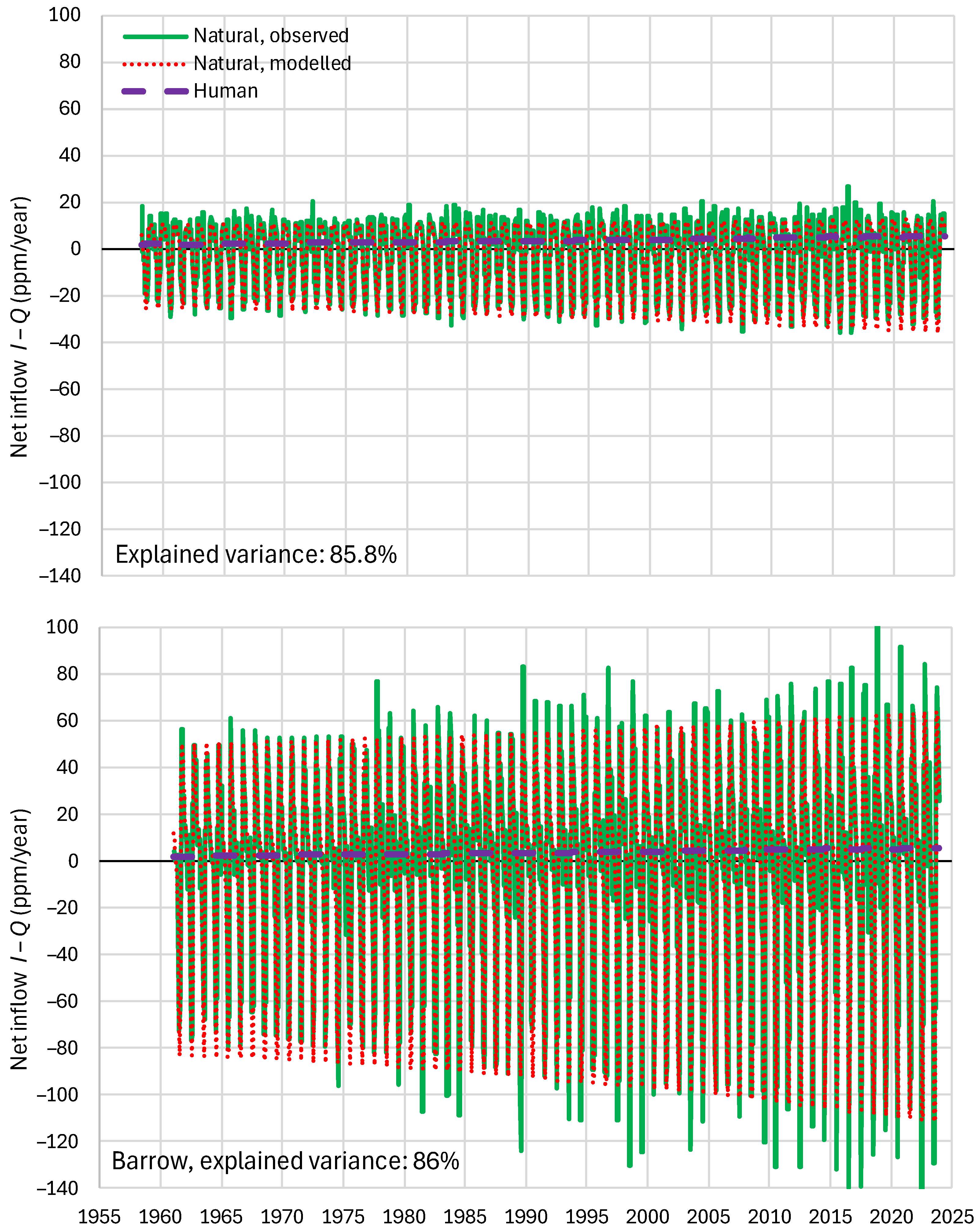
Figure 16.
Comparison of observed and simulated (upper) storages and (lower) net inflows for Barrow, in the case that the cosine function of inflow is replaced by an arbitrary function, defined through 24 coordinates.
Figure 16.
Comparison of observed and simulated (upper) storages and (lower) net inflows for Barrow, in the case that the cosine function of inflow is replaced by an arbitrary function, defined through 24 coordinates.
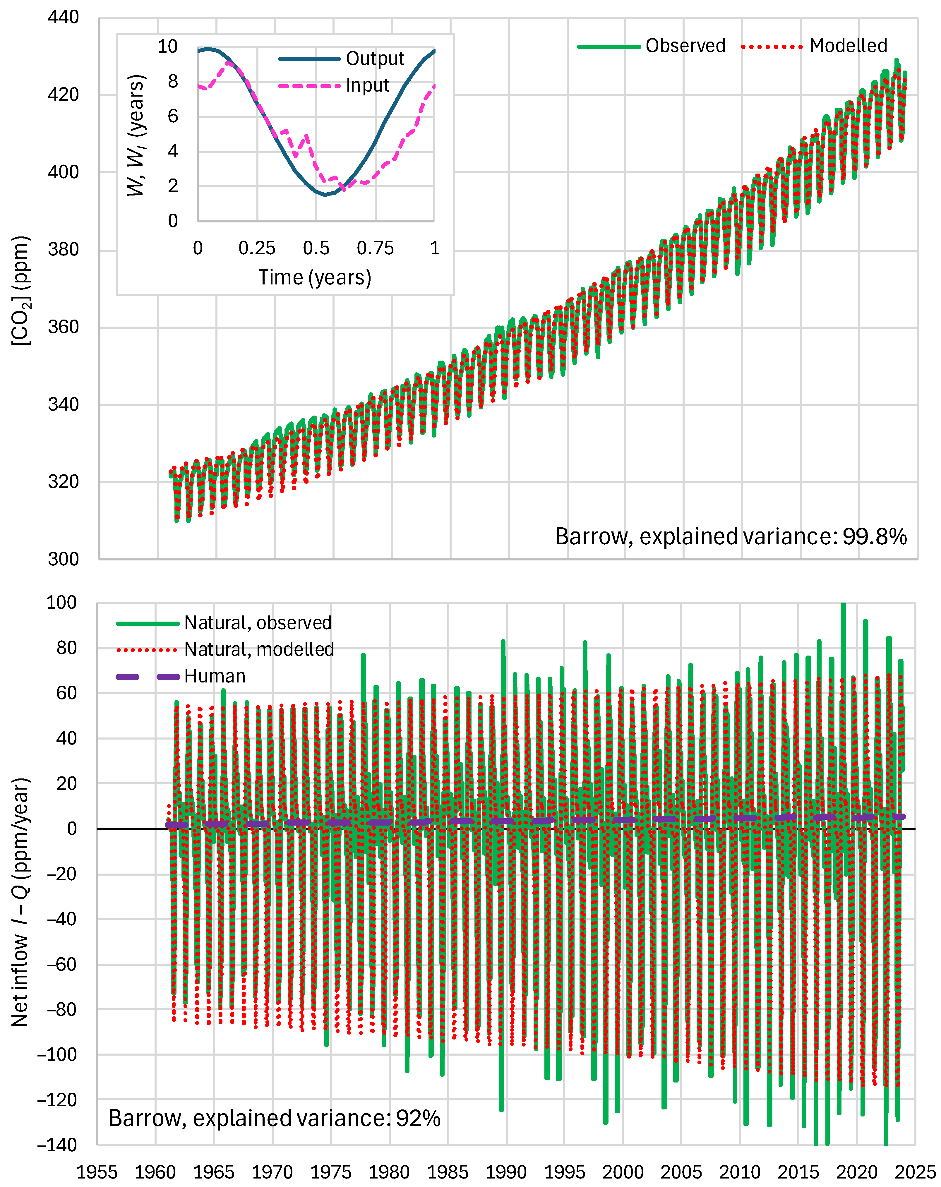
Figure 17.
Comparison of observed and simulated storage, , for (upper) Mauna Loa and (lower) Barrow, as in Figure 13, but omitting anthropogenic emissions (imaginary case 1). The insets show the seasonal variation of the characteristic times .
Figure 17.
Comparison of observed and simulated storage, , for (upper) Mauna Loa and (lower) Barrow, as in Figure 13, but omitting anthropogenic emissions (imaginary case 1). The insets show the seasonal variation of the characteristic times .
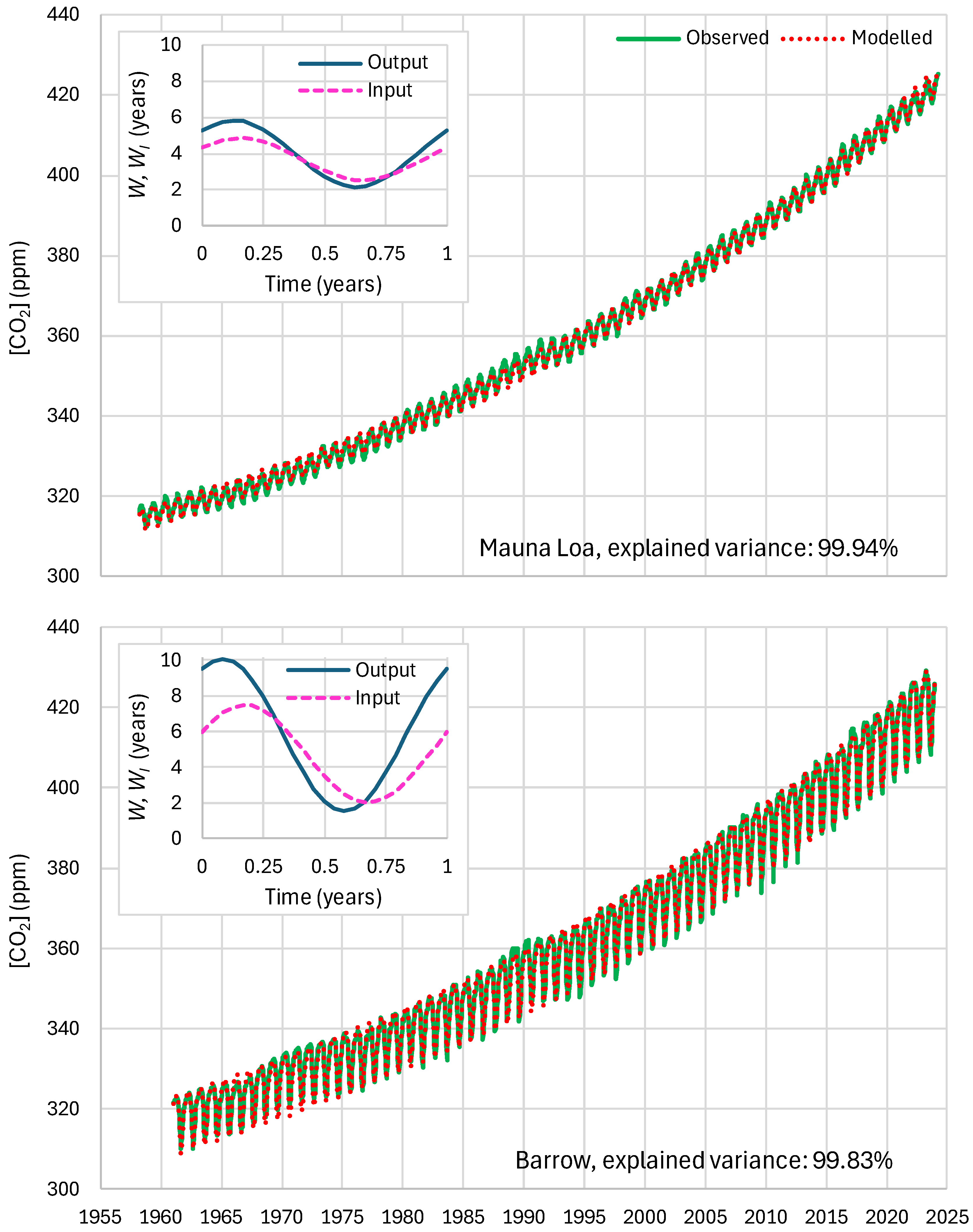
Figure 18.
Comparison of observed and simulated storage, , for (upper) Mauna Loa and (lower) Barrow, as in Figure 13 but for the indicated imaginary cases. The insets show the seasonal variation of the characteristic times for the case of all emissions without biosphere expansion (imaginary case 4). The explained variance noted is for the same case, while it is smaller in the other indicated cases, and decreased to less than –100% for the worst case of human emissions only.

Figure 19.
Comparison of observed and simulated net inflows for (upper) Mauna Loa and (lower) Barrow as in Figure 15 but without biosphere expansion (imaginary case 4).
Figure 19.
Comparison of observed and simulated net inflows for (upper) Mauna Loa and (lower) Barrow as in Figure 15 but without biosphere expansion (imaginary case 4).

Figure 20.
Comparison of observed and simulated storage, , as in Figure 13 but for the calibration period 1958–2002: (upper) Mauna Loa and (lower) Barrow. The insets show the seasonal variation of the characteristic times .
Figure 20.
Comparison of observed and simulated storage, , as in Figure 13 but for the calibration period 1958–2002: (upper) Mauna Loa and (lower) Barrow. The insets show the seasonal variation of the characteristic times .
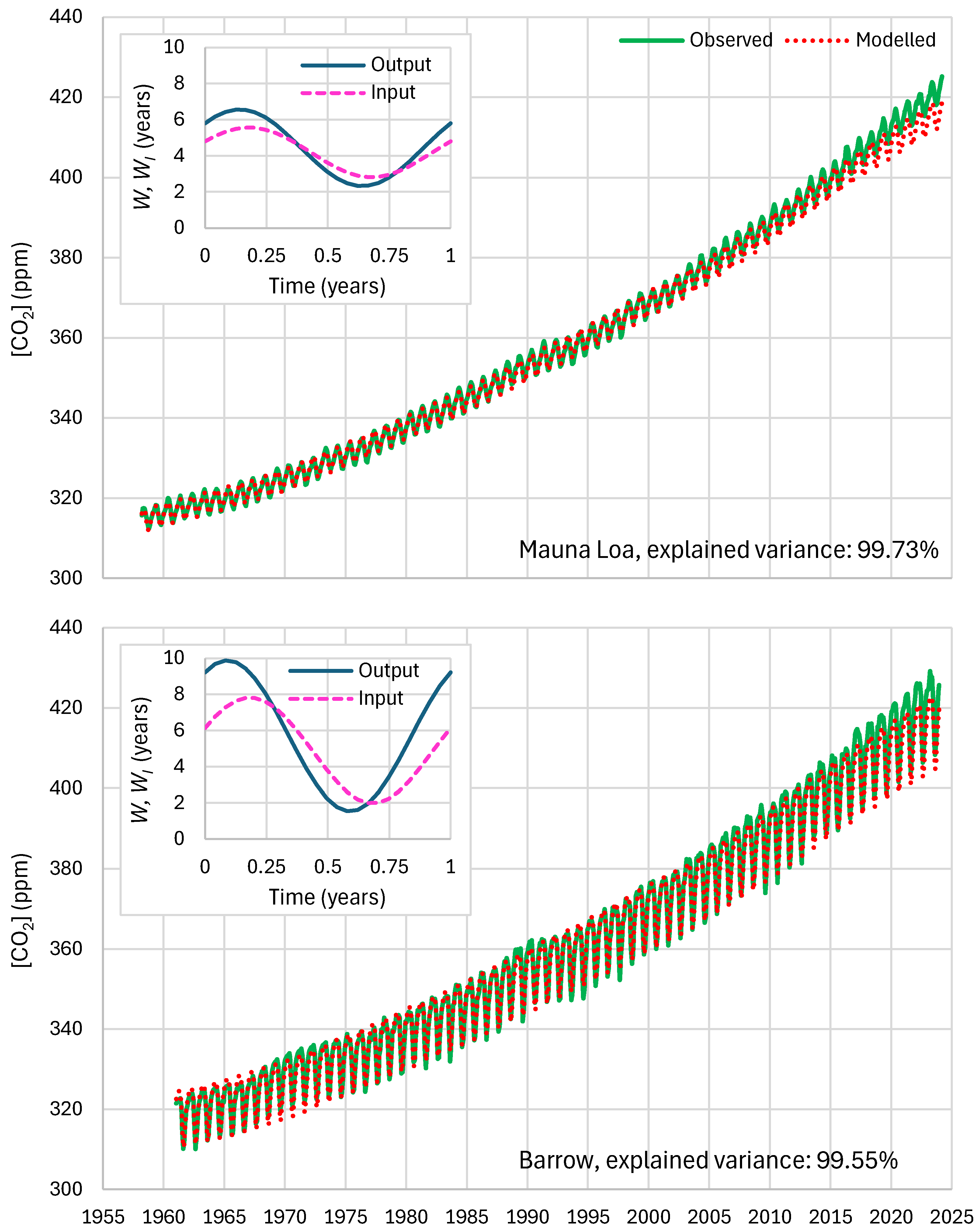
Figure 21.
Comparison of observed and simulated net inflows as in Figure 15 but for the calibration period 1958–2002: (upper) Mauna Loa and (lower) Barrow.
Figure 21.
Comparison of observed and simulated net inflows as in Figure 15 but for the calibration period 1958–2002: (upper) Mauna Loa and (lower) Barrow.
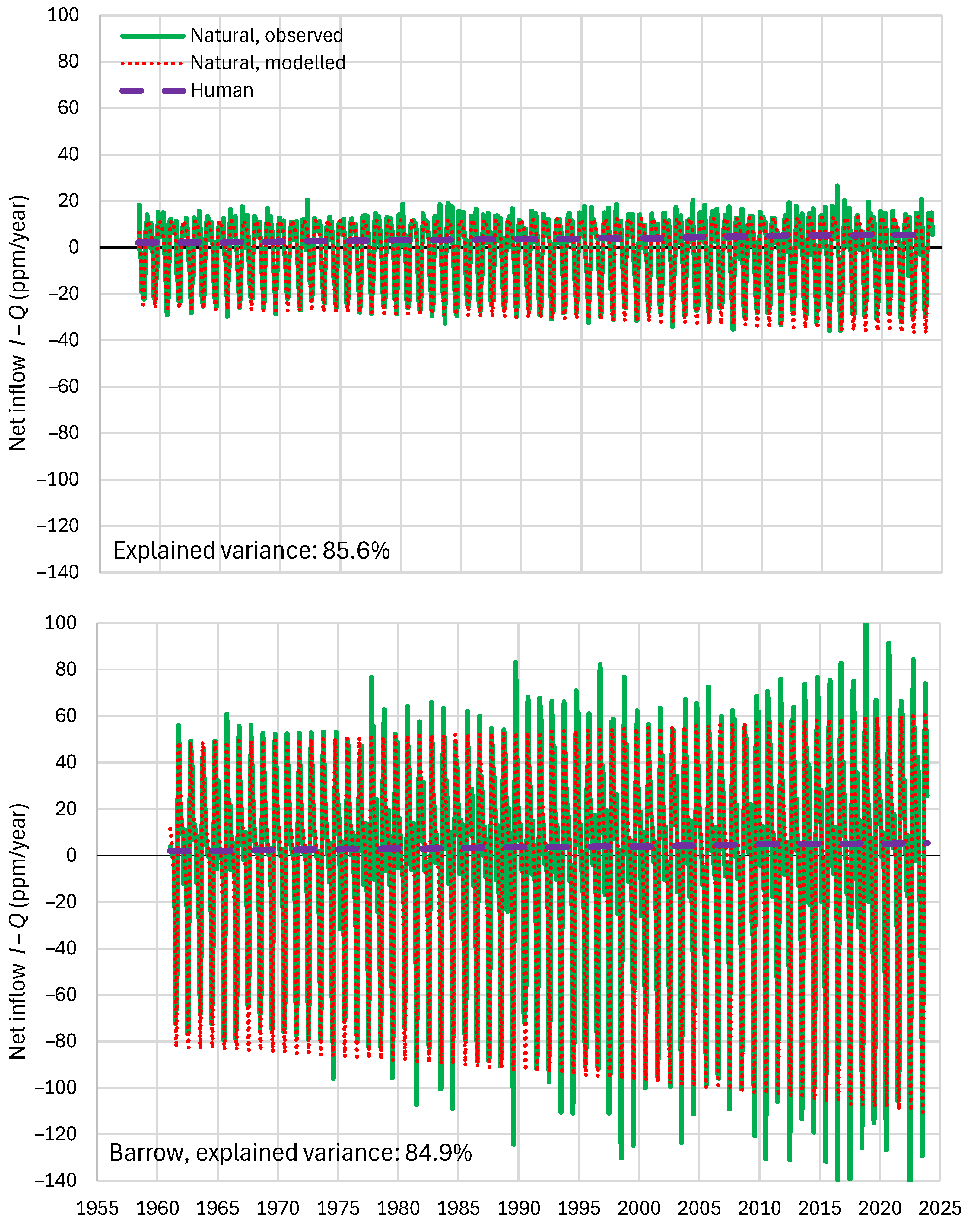
Table 1.
Fitted parameters of Equations (55) and (56).
| Site | (Years) | (Years) | ||||||
|---|---|---|---|---|---|---|---|---|
| Mauna Loa | 1 | 5.445 | 1.973 | 2.115 | 0.953 | 5.247 | 1.462 | 2.855 |
| Barrow | 1 | 5.757 | 4.181 | 1.370 | 0.953 | 5.149 | 3.104 | 1.633 |
Table 2.
Fitted parameters of Equations (55) and (56) as in Table 1 but for the calibration period 1958–2002. For comparison, the parameters of Table 1 are also shown in parentheses.
| Site | (Years) | (Years) | ||||||
|---|---|---|---|---|---|---|---|---|
| Mauna Loa | 1 | 5.399 (5.445) | 2.126 (1.973) | 2.092 (2.115) | 0.935 (0.953) | 5.164 (5.247) | 1.578 (1.462) | 2.858 (2.855) |
| Barrow | 1 | 5.710 (5.757) | 4.174 (4.181) | 1.368 (1.370) | 0.935 (0.953) | 5.134 (5.149) | 2.207 (3.104) | 1.594 (1.633) |
Table 3.
Explained variances (%) as performance indices of the RRR method for the indicated applications.
Table 3.
Explained variances (%) as performance indices of the RRR method for the indicated applications.
| ↓Site | (ppm) | (ppm/year) | ||||
|---|---|---|---|---|---|---|
| Period→ | All | 1958–2002 | 2003–2023 | All | 1958–2002 | 2003–2023 |
| Calibration over the entire period | ||||||
| Mauna Loa | 99.94 | 99.82 | 99.64 | 85.81 | 87.25 | 83.30 |
| Barrow | 99.77 | 99.25 | 99.16 | 85.30 | 85.82 | 84.64 |
| Calibration over the period 1958–2002 | ||||||
| Mauna Loa | 99.73 | 99.90 | 96.24 | 85.57 | 87.46 | 82.25 |
| Barrow | 99.55 | 99.44 | 95.88 | 84.85 | 86.18 | 83.13 |
Note: The arrow ↓ point to the column that follows and the → points to the row.
Table 4.
Mean residence times, seasonal () and annual (in years).
| Site | , Beginning Year | , Ending Year | ||||
|---|---|---|---|---|---|---|
| Calibration over the entire period | ||||||
| Mauna Loa | 2.20 | 6.15 | 4.17 | 3.68 | 3.68 | 3.70 |
| Barrow | 1.55 | 9.91 | 5.73 | 3.91 | 3.94 | 3.95 |
| Calibration over period 1958–2002 | ||||||
| Mauna Loa | 2.32 | 6.57 | 4.45 | 3.91 | 3.93 | 3.98 |
| Barrow | 1.53 | 9.88 | 5.70 | 3.89 | 3.92 | 3.98 |
Disclaimer/Publisher’s Note: The statements, opinions and data contained in all publications are solely those of the individual author(s) and contributor(s) and not of MDPI and/or the editor(s). MDPI and/or the editor(s) disclaim responsibility for any injury to people or property resulting from any ideas, methods, instructions or products referred to in the content. |
© 2024 by the author. Licensee MDPI, Basel, Switzerland. This article is an open access article distributed under the terms and conditions of the Creative Commons Attribution (CC BY) license (https://creativecommons.org/licenses/by/4.0/).
Share and Cite
MDPI and ACS Style
Koutsoyiannis, D. Refined Reservoir Routing (RRR) and Its Application to Atmospheric Carbon Dioxide Balance. Water 2024, 16, 2402. https://doi.org/10.3390/w16172402
AMA Style
Koutsoyiannis D. Refined Reservoir Routing (RRR) and Its Application to Atmospheric Carbon Dioxide Balance. Water. 2024; 16(17):2402. https://doi.org/10.3390/w16172402
Chicago/Turabian StyleKoutsoyiannis, Demetris. 2024. "Refined Reservoir Routing (RRR) and Its Application to Atmospheric Carbon Dioxide Balance" Water 16, no. 17: 2402. https://doi.org/10.3390/w16172402
Note that from the first issue of 2016, this journal uses article numbers instead of page numbers. See further details here.