Article

Characterization and Quantification of Dam Seepage Based on Resistivity and Geological Information

1
Hekoucun Reservoir Operation Center, Jiyuan 454650, China
2
Yellow River Engineering Consulting Co., Ltd., Zhengzhou 450003, China
3
School of Civil Engineering, Shandong University, Jinan 250061, China
*
Author to whom correspondence should be addressed.
Water 2024, 16(17), 2410; https://doi.org/10.3390/w16172410
Submission received: 19 July 2024 / Revised: 21 August 2024 / Accepted: 25 August 2024 / Published: 27 August 2024
(This article belongs to the Section Hydrogeology)

Abstract

:
Dam seepage significantly poses a serious threat to both the reservoir safety and the ecological health of the surrounding area. Characterizing and quantifying seepage zones is essential for effective risk mitigation and reinforcement measures. In this study, Electrical Resistivity Tomography (ERT) was applied to detect seepage on a reservoir dam. The ERT survey included three survey lines along the dam. The results indicated low resistivity in seepage zones, showing a distribution extending to the deep section in the middle of the dam and shallow section on both sides of the dam. The reservoir water came out to the ground surface in the downstream from seepage zones. Five seepage models were constructed to quantify seepage based on geological information. The models were further modeled based on the ERT results. Simulated results revealed the annual seepage of the reservoir is 78,880.16 m3. However, 75.5% of the total seepage is contributed by a region representing 50% of the dam. This concentrated seepage should draw the attention of future safety monitoring and reinforcement efforts. This study combines geophysics, geological, and numerical simulation to quantify dam seepage. This allows for the development of more scientifically sound solutions for preventing seepage and improving drainage ability in reservoir dams.

1. Introduction

Water resources are critical for healthy development of the economy and society. Reservoirs play a vital role in flood control, water supply, ecological balance, and power generation [1]. In the past century, numerous reservoirs have been constructed in China with the objective of enhancing the usage of water resources and mitigating the occurrence of water-related disasters [2,3]. However, these reservoirs frequently fail to meet current quality standards after years of operation due to funding and technology limitations [4].
Seepage can trigger the erosion of the dam structure, which is one of the main causes of reservoir failure [5,6,7]. Concentrated seepage channels have the potential to result in heterogeneous settlement of the dam body [8,9]. The unremitting deterioration of seepage will lead to water wastage, external submersion, and soil salinization, severely impacting the reservoir safety and ecological health of the surrounding area [10]. Therefore, detection of dam seepage is crucial for evaluating reservoir safety and implementing reinforcement efforts [11,12].
Seepage detection through borehole drilling and sampling is limited by the number of boreholes, which only provide localized information rather than continuous results. Moreover, the process of borehole drilling could potentially compromise the integrity of the original structure, thus worsening seepage issues [13,14]. Temperature measurements can be used to evaluate leakages, but this approach is also invasive [15,16]. The utilization of geochemical, isotopic, and tracer data has also been employed to identify seepage pathways, but this approach is associated with high costs, making it unsuitable for large-scale studies [17].
Geophysical methods have become an efficient and non-invasive means for detecting dam seepage and assessing its stability [18,19,20]. The ground-penetrating radar (GPR) method is a fast and reliable technique, although the penetration depth of electromagnetic waves at specific frequencies can be limited [21]. Geoelectrical methods are essential for identifying flow pathways through dams during seepage investigations [22,23,24]. The self-potential (SP) method is a commonly employed technique for the detection of dam seepage. However, the SP signal is often relatively weak, and the presence of other underground current sources can complicate data interpretation [25,26,27,28]. Electrical Resistivity Tomography (ERT) is particularly valuable for providing essential data in the assessment of seepage [29,30,31]. Numerous ERT studies in dam seepage detection and monitoring have fully demonstrated its effectiveness and benefits [32,33]. The combined use of techniques such as Electrical Resistivity Tomography and Fiber Bragg grating (FBG) shows promising results for seepage detection [34]. Long-term resistivity monitoring provides valuable insights into seepage development [35]. However, existing studies primarily focus on the alterations in resistivity caused by seepage and the localization of seepage pathways; there is a paucity of studies that simultaneously address both seepage localization and quantification issues [36]. Numerical simulations based on hydrogeological information allow for the quantitative estimation of seepage. However, the seepage models are limited by the number of boreholes [36]. The integration of geological data with resistivity results can facilitate the inference of more continuous sections. Furthermore, the correlation between seepage models and hydrogeological profiles can be established to make the quantitative results more reliable.
In this study, we explore a method for describing and quantifying dam seepage with geological and resistivity information. The resistivity method is combined with numerical simulation to characterize and quantitatively analyze dam seepage. An ERT survey is used to collect resistivity data of the dam. Seepage models are proposed to quantify seepage based on geological data, which are correlated to specific regions of the dam based on the ERT results. Numerical simulation results provide quantification of the spatial variations in seepage within these regions. In the end, we advocate for the integration of geophysical and geological datasets for comprehensive interpretation and detailed delineation of the seepage zones.

2. Materials and Methods

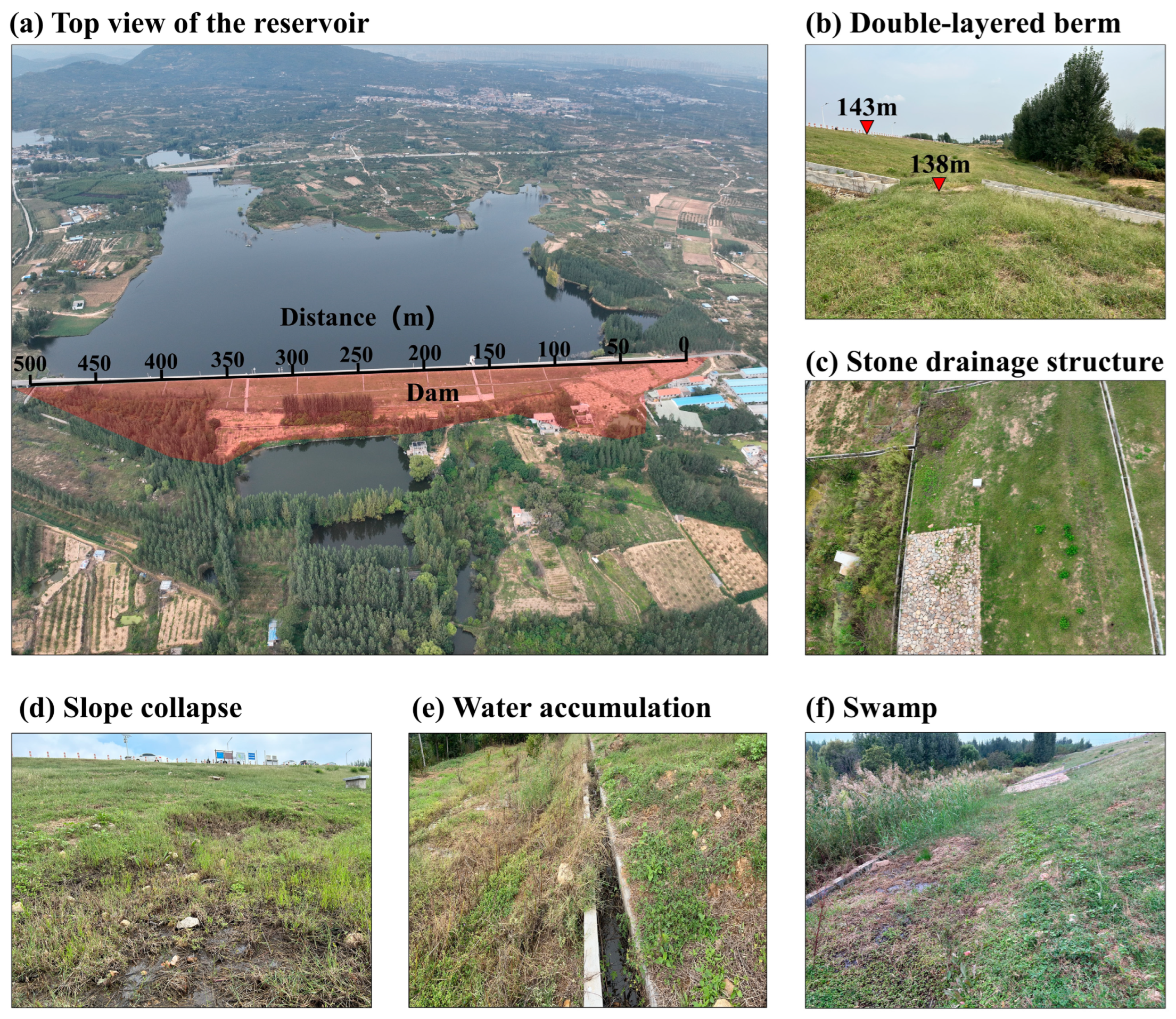
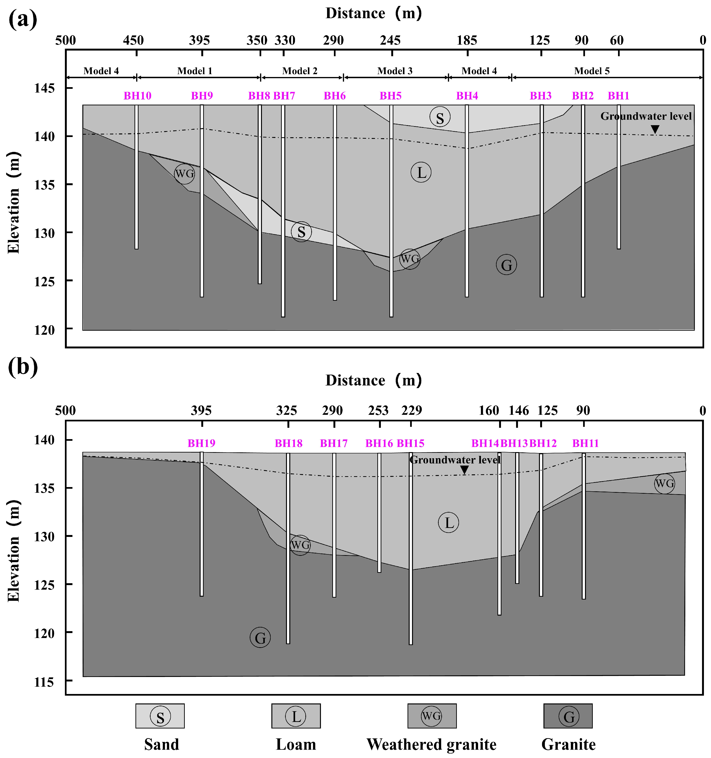
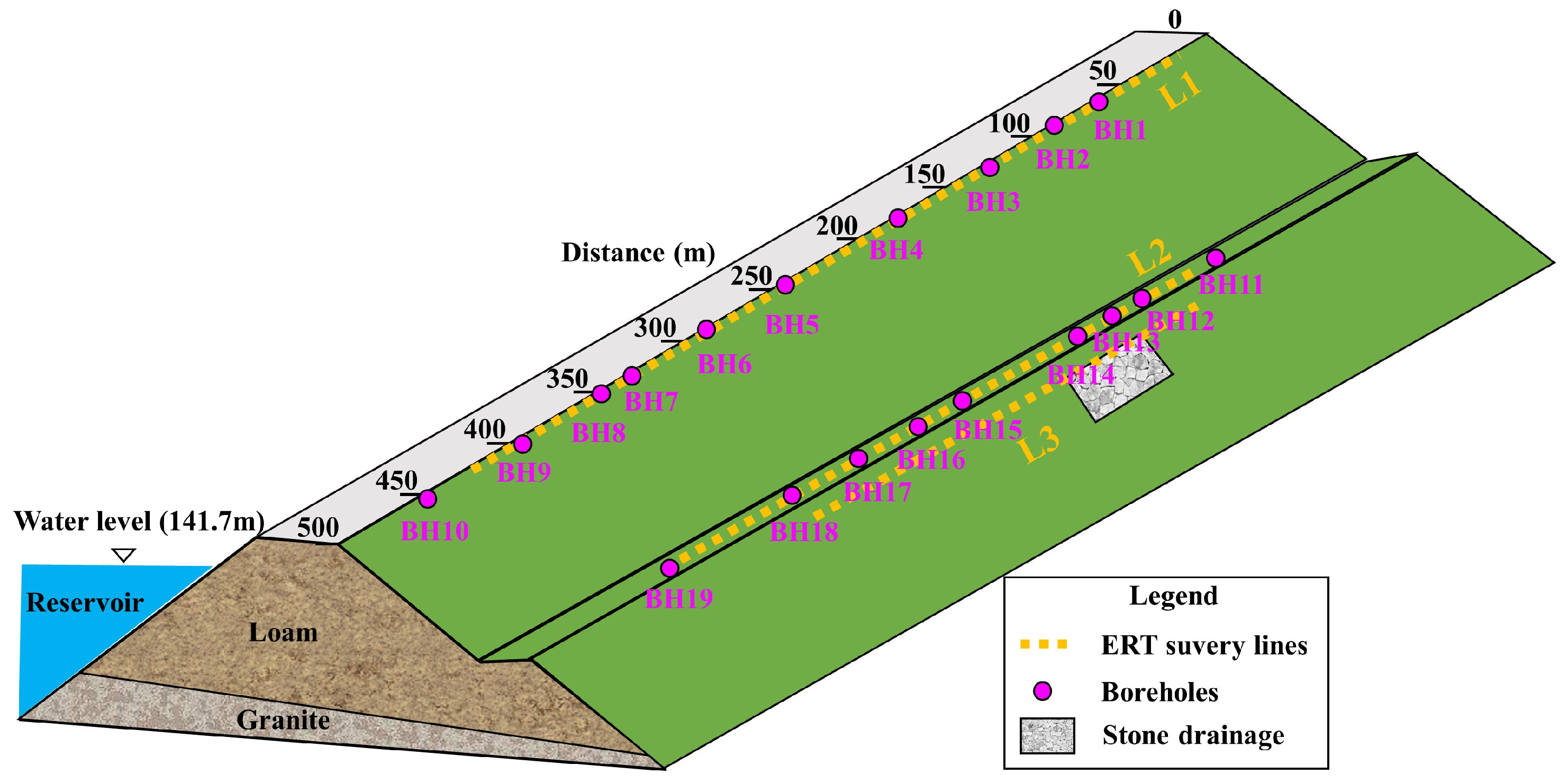
2.1. Site Description

The study was carried out on a heterogeneous embankment dam situated at the foothills of Mount Tai in eastern China (Figure 1a). The embankment spans 500 m in length, with masonry on the upstream and grass cover on the downstream. A double-layered berm was constructed on the downstream of the embankment to enhance stability (Figure 1b). The crest access road is elevated at 143 m, while the lateral berm stands at an elevation of 138 m. A stone drainage structure of 30 m in length was constructed on the slope of the dam to facilitate the discharge of seepage (Figure 1c). After more than decades of continuous operation, the downstream of the reservoir dam has developed abnormal seepage phenomena such as collapses (Figure 1d), water accumulation (Figure 1e), and a swamp (Figure 1f).
Figure 2 shows the geological profile in the downstream of the dam at elevations 143 m and 138 m. There are 19 boreholes that show the distribution of strata. The loam dam with sand lenses is situated above granite. The granite foundation exhibits localized weathering at the top. The thickness of the loam gradually increases from the sides towards the middle. The loam exhibits variations in hydraulic conductivity, ranging from 1.74 × 10⁻⁷ m/s to 4.72 × 10⁻⁶ m/s. The reservoir water level elevation was 141.7 m, and the groundwater depth ranged from 0 to 3 m. Due to the absence of anti-seepage measures, the seeping water flowed out in the areas below 136 m on the downstream.

2.2. Electrical Resistivity Tomography

As shown in Figure 3, three parallel ERT profiles were deployed to measure resistivity data using an ABEM Terrameter LS2 (Guideline Geo., Malå, Sweden) with gradient array. The roll-along method was used with a 3 m electrode spacing. The lengths/elevations of Profile 1, 2, and 3 are 381 m/143 m, 285 m/138 m, and 189 m/136 m. The injected current was 200 mA with 2 s current injection and 3 stacks. Profile 1, 2, and 3 collected 3528, 2450, and 1372 quadrupoles in total.
Following the manual removal of negative data points and outliers along pseudo sections, the data points used for inversion on Profiles 1, 2, and 3 accounted for over 99.7%, with 3520, 2446, and 1368 data points left, indicating the high quality of the ERT data. Therefore, measurement errors in the data were not considered during the inversion process, even though estimating these errors can lead to superior inversion results and more accurate uncertainty estimates in synthetic examples [37]. Pseudo-sections were inverted with RES2DINV (v4.08) based on a finite-element approach [38]. The thickness of the first layer employed in the inversion model was 0.5 times the electrode spacing, with each subsequent layer increasing in thickness by 10% relative to the previous layer. The robust inversion (L1-norm) method was used to sharpen the boundary between the loam and the granite. There were two cut-off factors that needed to be set to control the robust inversion. One cut-off factor controls the extent to which this robust data constraint is applied. We used a value of 0.05, meaning that the effect of data points where the differences in the measured and calculated apparent resistivity values were much greater than 5% would be greatly reduced. The other cut-off factor controls the degree of the robust model constraint. We used a value of 0.005, meaning that the result was close to the true L1-norm inversion method. [39]. After a maximum of 7 iterations, the relative change in RMS error was less than 1%. A lower RMS value indicates a better fit to the data.

2.3. Numerical Modeling of Seepage

As shown in Figure 2, the dam is composed of sand, loam, weathered granite, and granite. Based on the geological information, five representative locations at distance 395 m, 330 m, 245 m, 185 m, and 90 m were selected. Five seepage models were established using the Seep/w module in Geostudio software (2022.1) [40]. These five types of seepage models encompass all types of stratigraphic distribution in the geological profile. As shown in Figure 4, the seepage models at distance 395 m (model 1), 245 m (model 3), and 90 m (model 5) represent various thicknesses of weathered granite layers at different positions beneath the loam. The seepage model at distance 330 m (model 2) features a sand lens in the loam. At a distance of 185 m (model 4), the seepage model shows the loam with sand lenses is located on the granite.
The dimensions of all five 2D models are 75 m × 43 m. In these models, the upstream boundary is specified with a constant hydraulic head determined by the reservoir water level, while the downstream boundary is set as a seepage face. Based on the borehole data, the hydraulic conductivity of sand and granite were set to 1.184 m/d and 0.001 m/d. At distances of 395 m and 90 m, the hydraulic conductivity of loam and weathered granite were set to 0.182 m/d and 0.043 m/d, while at distances of 330 m, 245 m, and 185 m, they were set to 0.363 m/d and 0.062 m/d. All the models employ a discretized finite element cell size of 1 m for stable flow analysis.

3. Results

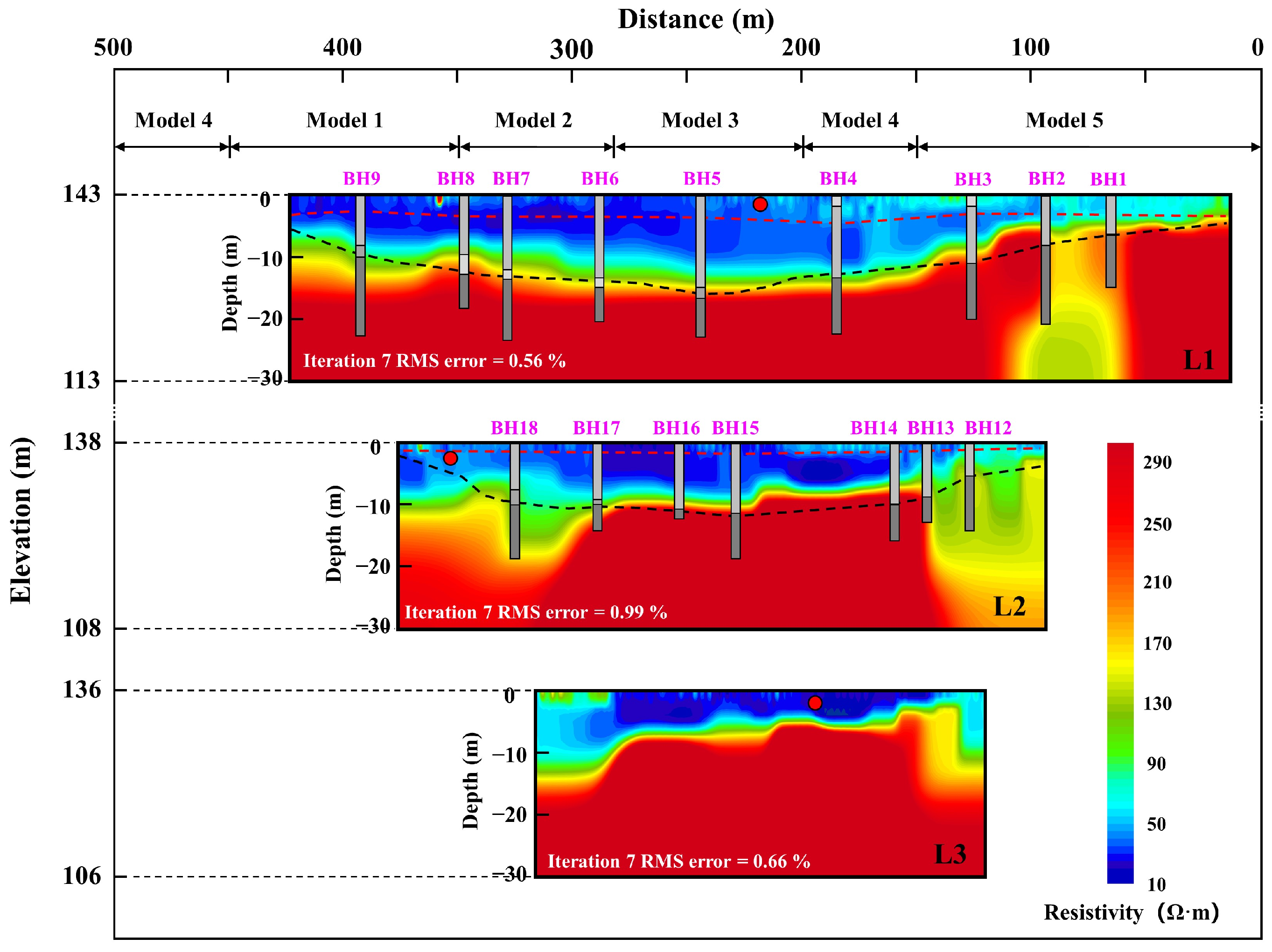
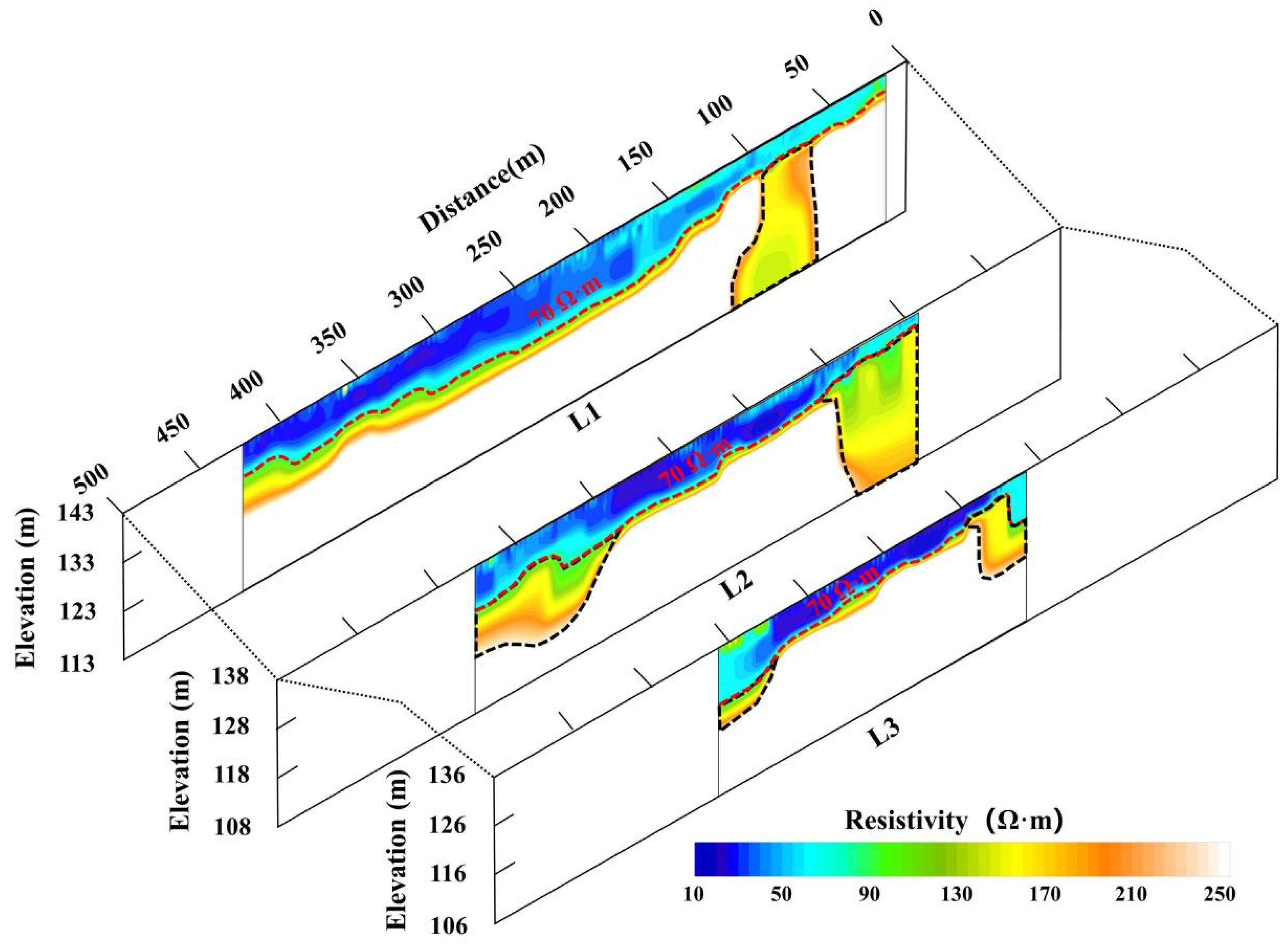
3.1. ERT Survey Results

The inversion results of three ERT survey profiles are shown in Figure 5. The elevation in the profiles is consistent with the geological profile. The red and black dashed lines are marked to indicate the elevations of groundwater levels and the top boundary of granite for reference. To demonstrate the correlation between resistivity values and the observed geological strata, data from sixteen boreholes are referenced in L1 and L2. The ERT data align well with the borehole information. The resistivity profiles of the three survey lines demonstrate a consistent low–to–high resistivity distribution from top to bottom, reflecting the distribution of loam, weathered granite, and granite. The granite below an elevation of 128 m exhibited a high resistivity response exceeding 250 Ω·m, while the sand and loam showed a low resistivity response at elevations between 143 and 128 m. The resistivity of the loam dam was less than 70 Ω·m, whereas that of the sand and the weathered granite ranged from 70 Ω·m to 250 Ω·m. The results show a significant difference in the resistivity values between sand and loam. In profile P1, the resistivity of sand from a distance of 100 m to 250 m exceeded 50 Ω·m, whereas the resistivity of loam beneath the sand was less than 50 Ω·m. To provide a more detailed explanation for the observed resistivity variations across the strata, three soil samples were collected from these profiles for laboratory analysis. The samples included one sand and two loam samples, with their respective locations depicted in Figure 5. As shown in Table 1, laboratory measurements revealed that the resistivity values for sand and loam were 263.2 Ω·m and 28.9/43.1 Ω·m, aligning well with the field results. As the elevation of the survey line decreased, the maximum thickness of the loam dam decreased from 15 m in profile P1 to 10 m in profile P2, and then to 8 m in profile P3. However, the elevation of the loam layer bottom remained around 128 m, consistent with the geological profiles.
It should be noted that the granite boundaries used as references were obtained based on a limited number of boreholes and the inversion grid was not divided according to the stratum boundaries. Therefore, there exists a discrepancy between the top boundary of the granite and the resistivity results, despite their general alignment in trend. In addition, the borehole data revealed varying degrees of weathering at the upper part of the granite, explaining the region where resistivity values ranged from 50 Ω·m to 200 Ω·m in the transition zone between loam and granite. Furthermore, the impact of precipitation during the survey period obscured the distinction between soil resistivity near the ground surface and below the groundwater level.

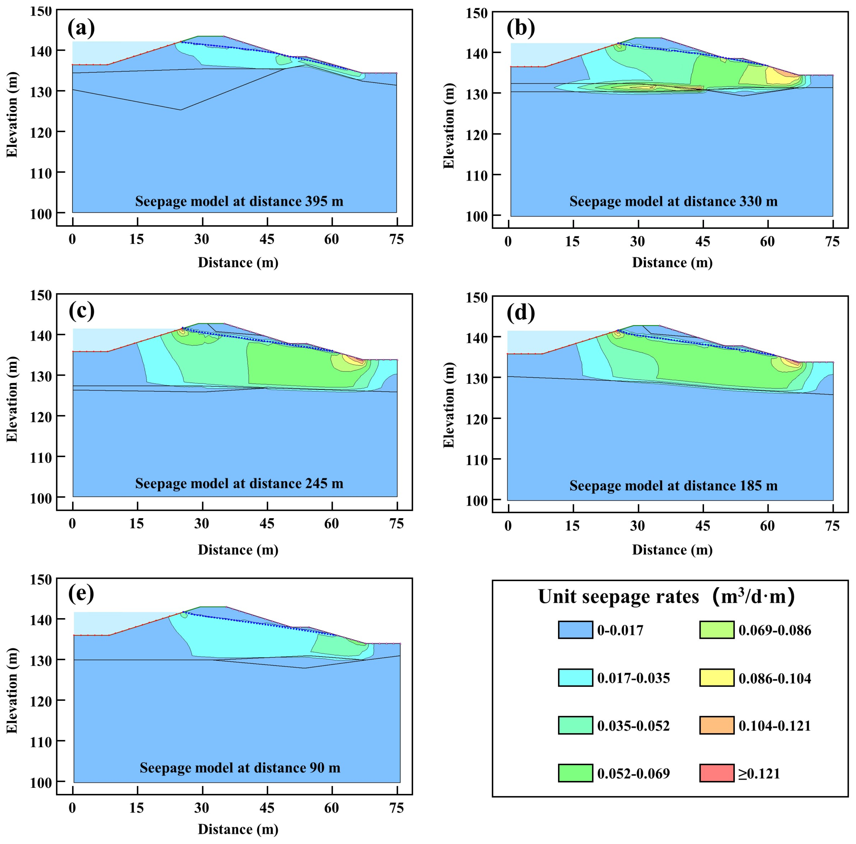
3.2. Seepage Simulation Results

In numerical simulation, the seepage entering the grid was positive, and that exiting the grid was negative, both with equal magnitudes in absolute terms. The sum of the seepage rates for all grids at a specified location was equal to the total seepage rate through that cross-section. Based on the model width and grid spacing, the unit seepage rate, i.e., the quantity of seepage flow per unit width, through each cross-section could be calculated. The calculated results of the five seepage models are shown in Figure 6. The results indicate that due to the low permeability of the granite, seepage was primarily concentrated in the loam and sand layers above the granite, with unit seepage rates ranging from 0.017 m3/d·m to 0.121 m3/d·m. The seepage rates in the granite were less than 0.017 m3/d·m, while they gradually increased from upstream to downstream in the loam layer, reaching a maximum of 0.121 m3/d·m beneath the berm on the downstream. Based on Darcy’s Law, the seepage rate is linearly related to the hydraulic conductivity. In Models 2, 3, and 4, the hydraulic conductivity of the loam was about twice that of models 1 and 5, causing the unit seepage rate to rise from 0–0.052 m3/d·m in Model 1 to 0–0.121 m3/d·m in Model 3. Therefore, due to the differences in hydraulic conductivity, the seepage rates in the central area of the dam (Model 2, Model 3, and Model 4) were significantly higher than those in the flanking areas (Model 1 and Model 5). The statistical results of the five seepage models are shown in Table 2. The unit seepage rate for Model 3 was 0.759 m3/d·m, which is 4.27 times the unit seepage rate of Model 1. This reflects the relatively higher permeability of the stratum in this area and the concentration of main seepage zones in the central part of the dam. The high-seepage areas mentioned above should be given particular attention.
The groundwater level obtained from the numerical simulation is marked with a blue dashed line in Figure 6. The results show that the groundwater level dropped from the reservoir water level of 141.7 m to the downstream berm and seeped out. This trend corresponds to the collapse, water accumulation, and swamp observed on the downstream, as shown in Figure 1.

4. Discussion

4.1. Localization of Seepage

As shown in Figure 5, the resistivity values on both sides of the loam are slightly higher than those in the middle region. For instance, along profile P2, the resistivity values from 89 m to 170 m and from 300 m to 377 m are higher than those between 170 m and 300 m. This reflects the distribution of permeability in the loam layer as revealed by borehole data, and the permeability on both sides is lower than that in the middle section. From 89 m to 150 m and from 300 m to 377 m along profile P2, the resistivity values of the underlying layers range between 70 Ω·m and 250 Ω·m, indicating the presence of weathered granite or sand, which is consistent with the geological profile. However, due to the limited number and depth of boreholes, there is a possibility of inaccuracies in the continuous representation of stratigraphy. Therefore, along profile P1 from 50 m to 120 m, the estimated resistivity depicts a larger area of weathered granite.
The loam and sand layers exhibit low resistivity and have higher seepage rates, whereas granite shows high resistivity and low seepage rates. Therefore, the loam and sand layers should be the seepage zones in the study area, with resistivity values less than 250 Ω·m. The resistivity values and hydraulic conductivity of weathered granite fall between those of loam and granite. Weathered granite exhibits uneven permeability distribution due to varying degrees of weathering. The seepage flow in this layer is less pronounced, but with the rise of reservoir water level and the enhancement of weathering, the seepage flow has the potential for further development. As shown in Figure 7, a detailed delineation of the seepage zones was obtained after filtering out the granite strata with resistivity values greater than 250 Ω·m.
The seepage zones were defined with resistivity values below 70 Ω·m. From 150 m to 300 m of profile P3, the seepage zone was observed to be in close proximity to the ground surface, indicating that seepage came out to the ground surface. This is consistent with the field situations shown in Figure 1. As shown in Figure 7, potential seepage zones are outlined with black dashed lines with resistivity values between 70 Ω·m and 250 Ω·m. These zones are predominantly distributed on both sides of the dam. The resistivity results reveal a wider range of weathered granite than that indicated by boreholes. The distribution of weathered granite needs to be further verified because the small number of boreholes affect the accuracy of geological profile generation.

4.2. Quantification of Seepage

Based on the resistivity results, it is possible to delineate the locations of seepage zones. However, accurately determining the seepage volume in these areas remains challenging. Meanwhile, seepage simulations are restricted by the limited number of boreholes. By combining resistivity results and geological data, continuous geological profiles can be inferred to provide a more detailed delineation of the regions represented by each model. To further quantify the spatial variations in seepage within the study area, the dam was divided into five regions based on geological information and resistivity results. This allowed for the identification of different distribution characteristics of sand, loam, and weathered granite layers. As shown in Table 2, Model 1–Model 5 represent sections of the dam with lengths of 100 m (350 m to 450 m), 70 m (280 m to 350 m), 80 m (200 m to 280 m), 100 m (150 m to 200 m and 450 m to 500 m), and 150 m (0 m to 150 m).
As shown in Figure 2 and Figure 5, the resistivity results and geological profiles show that the resistivity values and strata distribution in the representative areas of each model exhibit the same characteristics. In the representative area of Model 1, resistivity results and geological profiles show the weathered granite exists between the low-resistivity loam layer and the high-resistivity granite. An obvious resistivity characteristic of the representative area for Model 2 is the presence of a sand layer between the loam and granite. The resistivity results and the geological profile reveal weathered granite near the upstream position in the representative area for Model 3, whereas weathered granite is located closer to the downstream area in Model 5. In the representative area for Model 4, resistivity results show a sharp interface, indicating the absence of weathered granite. Therefore, these five models are representative of the entire dam. Limitations and potential sources of error in geological profiles include the reliance on limited borehole data, which may not capture all subsurface variability, leading to incomplete profiles and inaccurate seepage models. Simplifying complex geological features for computational ease may result in less precise seepage predictions. However, the site in this study has only four types of strata, and their distribution is not complex, so our simplified approach is suitable. Moreover, we used resistivity information to integrate and classify the geological profiles, rather than relying solely on borehole data.
The numerical results reveal a detailed seepage distribution. Based on the representative length of each region, the annual total seepage volume of the dam was calculated to be 78,880.15 m3. This is equivalent to 3.73% of the total reservoir capacity and 5.18% of the effective reservoir capacity. However, the section between 100 m and 350 m constitutes only half of the total dam length yet accounts for 75.08% of the annual seepage in the entire reservoir. The concentrated seepage area should become the focal point of dam safety monitoring and subsequent reinforcement.
By integrating resistivity data with geological information, our approach enables the delineation of overall geological conditions using limited borehole data. This integration allows our seepage model to correspond with these profiles, highlighting the crucial role of ERT in zonal seepage quantification. We used a limited number of boreholes and modeling to describe seepage, complementing this with ERT and geological information to address gaps between models. This method is particularly advantageous for dams with minimal stratigraphic variation and sparse borehole data. For dams with more comprehensive geological and monitoring data, extensive 2D seepage models and 3D numerical simulations yield more accurate results.

5. Conclusions

This study used the ERT method to delineate seepage zones in the reservoir dam. These seepage zones were defined by resistivity results and geological information. Five representative seepage models were established according to geological and geophysical information to accurately quantify the seepage volumes within the dam. The main conclusions are summarized as follows:
The seepage zones of the dam body are primarily located in the loam on the top of the granite strata. The area between 100 m and 350 m accounts for 75.08% of the annual seepage of the dam. This concentrated seepage is primarily attributable to the variable thickness and permeability of the loam layers.
ERT can be used for routine detection of seepage zones in reservoir dams. However, integrating the geophysical results with hydrogeological information is essential for accurately delineating seepage areas. Geophysical methods remain a cost-effective technique for safety inspection and monitoring of reservoir dams at present. The integrated use of geological, geophysical, and numerical simulation methods can scientifically and reasonably divide the research area and accurately quantify seepage.
The method proposed in this study combines resistivity, geological information, and seepage simulations, improving both the reliability of geophysical findings and the quantifiability of detection outcomes. This study provides data support for the safety assessment and reinforcement of reservoir dams and offers a basis for developing seepage prevention and drainage solutions. This integrated method can be applied to various hydraulic engineering scenarios such as river embankments and water transfer channels, demonstrating its broad applicability.
This method can describe and quantify dam seepage with little geological and resistivity information. To further enhance the accuracy and applicability of ERT and numerical simulation methods in dam seepage studies, we offer the following recommendations for future research: (a) explore time-lapse and joint inversion methods for better subsurface modeling and its evolution over time, (b) correct the model using data from boreholes and reservoir water level monitoring, (c) adopt 3D ERT modeling to capture the full complexity of seepage processes, and (d) improve numerical simulation models by incorporating transient conditions.

Author Contributions

Conceptualization, D.M.; methodology, D.M.; software, D.M.; validation, J.L.; formal analysis, J.J.; investigation, Y.W.; resources, J.J.; data curation, L.S.; writing—original draft preparation, Y.W.; writing—review and editing, Y.W.; visualization, J.W.; supervision, J.J.; project administration, Q.G.; funding acquisition, J.W. All authors have read and agreed to the published version of the manuscript.

Funding

This research was funded by Water Conservancy Science and Technology Research Project of Henan Provincial Water Resources Department, grant number GG202136, Henan Provincial Science and Technology Research Project, grant number 232102320314, and Independent Research and Development Project of Yellow River Engineering Consulting Co., Ltd.

Data Availability Statement

The raw data supporting the conclusions of this article will be made available by the authors on request.

Conflicts of Interest

Authors Qifeng Guo, Junzhi Wang and Lu Sun were employed by the company Yellow River Engineering Consulting Co., Ltd. The remaining authors declare that the research was conducted in the absence of any commercial or financial relationships that could be construed as a potential conflict of interest.

References

  1. Shen, Y.; Chen, Y. Global perspective on hydrology, water balance, and water resources management in arid basins. Hydrol. Process. 2010, 24, 129–135. [Google Scholar] [CrossRef]
  2. Wen, F.; Guan, W.H.; Yang, M.X.; Cao, J.X.; Zou, Y.B.; Liu, X.; Wang, H.J.; Dong, N.P. The Optimization of Water Storage Timing in Upper Yangtze Reservoirs Affected by Water Transfer Projects. Water 2023, 15, 3393. [Google Scholar] [CrossRef]
  3. Men, B.H.; Liu, H.L.; Tian, W.; Wu, Z.J.; Hui, J. The Impact of Reservoirs on Runoff Under Climate Change: A Case of Nierji Reservoir in China. Water 2019, 11, 1005. [Google Scholar] [CrossRef]
  4. Miao, C.Y.; Borthwick, A.G.L.; Liu, H.H.; Liu, J.G. China’s Policy on Dams at the Crossroads: Removal or Further Construction? Water 2015, 7, 2349–2357. [Google Scholar] [CrossRef]
  5. Cho, I.K.; Yeom, J.Y. Crossline resistivity tomography for the delineation of anomalous seepage pathways in an embankment dam. Geophysics 2007, 72, 31–38. [Google Scholar] [CrossRef]
  6. Hung, Y.C.; Chen, T.T.; Tsai, T.F.; Chen, H.X. A Comprehensive Investigation on Abnormal Impoundment of Reservoirs—A Case Study of Qionglin Reservoir in Kinmen Island. Water 2021, 13, 1463. [Google Scholar] [CrossRef]
  7. Foster, M.; Fell, R.; Spannagle, M. The statistics of embankment dam failures and accidents. Can. Geotech. J. 2000, 37, 1000–1024. [Google Scholar] [CrossRef]
  8. Richards, K.S.; Reddy, K.R. Experimental investigation of initiation of backward erosion piping in soils. Geotechnique 2012, 62, 933–942. [Google Scholar] [CrossRef]
  9. Jiang, T.; Zhang, J.R.; Wan, W.F.; Cui, S.; Deng, D.P. 3D transient numerical flow simulation of groundwater bypass seepage at the dam site of Dongzhuang hydro-junction. Eng. Geol. 2017, 231, 176–189. [Google Scholar] [CrossRef]
  10. Rozycki, A.; Fonticiella, J.M.R.; Cuadra, A. Detection and evaluation of horizontal fractures in earth dams using the self-potential method. Eng. Geol. 2006, 82, 145–153. [Google Scholar] [CrossRef]
  11. Song, S.H.; Song, Y.; Kwon, B.D. Application of hydrogeological and geophysical methods to delineate leakage pathways in an earth fill dam. Explor. Geophys. 2005, 36, 92–96. [Google Scholar] [CrossRef]
  12. Lin, C.P.; Hung, Y.C.; Wu, P.L.; Yu, Z.H. Performance of 2-D ERT in investigation of abnormal seepage: A case study at the Hsin-Shan earth dam in Taiwan. J. Environ. Eng. Geophys. 2014, 19, 101–112. [Google Scholar] [CrossRef]
  13. Xia, T.; Meng, J.; Ding, B.T.; Chen, Z.F.; Liu, S.L.; Titov, K.; Mao, D.Q. Integration of hydrochemical and induced polarization analysis for leachate localization in a municipal landfill. Waste Manag. 2023, 157, 130–140. [Google Scholar] [CrossRef]
  14. Hu, Z.H.; Wang, Y.X.; Ye, M.S.; Liu, M.; Ding, J.Q. Localization of potential leakage areas inside plain reservoirs using waterborne electrical resistivity tomography. J. Environ. Eng. Geophys. 2021, 26, 133–143. [Google Scholar] [CrossRef]
  15. Yun, T.; Karl, E.B.; MacQuarrie, K.T.B. Investigation of seepage near the interface between an embankment dam and a concrete structure: Monitoring and modelling of seasonal temperature trends. Can. Geotech. J. 2023, 60, 453–470. [Google Scholar] [CrossRef]
  16. Khan, A.A.; Vrabie, V.; Beck, Y.L.; Mars, I.J.; DUrso, G. Monitoring and early detection of internal erosion: Distributed sensing and processing. Struct. Health Monit. 2014, 13, 562–576. [Google Scholar] [CrossRef]
  17. McMahon, P.B.; Carney, C.P.; Poeter, E.P.; Peterson, S.M. Use of geochemical, isotopic, and age tracer data to develop models of groundwater flow for the purpose of water management, northern High Plains aquifer. Appl. Geophys. 2010, 25, 910–922. [Google Scholar] [CrossRef]
  18. Ling, C.; Revil, A.; Abdulsamad, F.; Qi, Y.; Ahmed, A.S.; Shi, P.; Nicaise, S.; Peyras, L. Leakage detection of water reservoirs using a Mise-à-la-Masse approach. J. Hydrol. 2019, 572, 51–65. [Google Scholar] [CrossRef]
  19. Ikard, S.J.; Rittgers, J.; Revil, A.; Mooney, M.A. Geophysical Investigation of Seepage Beneath an Earthen Dam. Groundwater 2015, 53, 238–250. [Google Scholar] [CrossRef]
  20. Hu, Z.H.; Liu, M.; Wang, Y.X.; Ye, M.S.; Li, S.X. Geophysical Assessment of Freshwater Intrusion into Saline Aquifers Beneath Plain Reservoirs. J. Environ. Eng. Geophys. 2022, 27, 13–22. [Google Scholar] [CrossRef]
  21. Di Prinzio, M.; Bittelli, M.; Castellarin, A.; Rossi Pisa, P. Application of GPR to the monitoring of river embankments. J. Appl. Geophys. 2010, 71, 53–61. [Google Scholar] [CrossRef]
  22. Daily, W.; Ramirez, A.; Binley, A. Remote Monitoring of Leaks in Storage Tanks using electrical resistance tomography: Application at the Hanford site. J. Environ. Eng. Geophys. 2004, 9, 11–24. [Google Scholar] [CrossRef]
  23. Golebiowski, T.; Piwakowski, B.; Cwiklik, M.; Bojarski, A. Application of Combined Geophysical Methods for the Examination of a Water Dam Subsoil. Water 2021, 13, 2981. [Google Scholar] [CrossRef]
  24. Antoine, R.; Fauchard, C.; Fargier, Y.; Durand, E. Detection of leakage areas in an earth embankment from GPR measurements and permeability logging. Int. J. Geophys. 2015, 2015, 610172. [Google Scholar] [CrossRef]
  25. Bolève, A.; Revil, A.; Janod, F.; Mattiuzzo, J.L.; Fry, J.-J. Preferential fluid flow pathways in embankment dams imaged by self-potential tomography. Near Surf. Geophys. 2009, 7, 447–462. [Google Scholar] [CrossRef]
  26. Revil, A.; Cary, L.; Fan, Q.; Finizola, A.; Trolard, F. Self-potential signals associated with preferential ground water flow pathways in a buried paleo-channel. Geophys. Res. Lett. 2005, 32, L07401. [Google Scholar] [CrossRef]
  27. Ahmed, A.S.; Revil, A.; Steck, B.; Vergniault, C.; Jardani, A.; Vinceslas, G. Self-potential signals associated with localized leaks in embankment dams and dikes. Eng. Geol. 2019, 253, 229–239. [Google Scholar] [CrossRef]
  28. Ikard, S.J.; Carroll, K.C.; Rucker, D.F.; Adams, R.F.; Brooks, S.C. Geoelectric characterization of hyporheic exchange flow in the bedrock-lined streambed of East Fork Poplar Creek, Oak Ridge, Tennessee. Geophys. Res. Lett. 2023, 50, e2022GL102616. [Google Scholar] [CrossRef]
  29. Cardarelli, E.; Cercato, M.; De Donno, G. Characterization of an earth-filled dam through the combined use of electrical resistivity tomography, P- and SH-wave seismic tomography and surface wave data. J. Appl. Geophys. 2014, 106, 87–95. [Google Scholar] [CrossRef]
  30. Fargier, Y.; Lopes, P.S.; Fauchard, C.; François, D.; Côte, P. DC-electrical resistivity imaging for embankment dike investigation: A 3D extended normalization approach. J. Appl. Geophys. 2014, 103, 245–256. [Google Scholar] [CrossRef]
  31. Perri, M.T.; Boaga, J.; Bersan, S.; Cassiani, G.; Cola, S.; Deiana, R.; Simonini, P.; Patti, S. River embankment characterization: The joint use of geophysical and geotechnical techniques. J. Appl. Geophys. 2014, 11, 5–22. [Google Scholar] [CrossRef]
  32. Loperte, A.; Soldovieri, F.; Lapenna, V. Monte Cotugno dam monitoring by the electrical resistivity tomography. IEEE J. Sel. Top. Appl. Earth Obs. Remote Sens. 2015, 8, 5346–5351. [Google Scholar] [CrossRef]
  33. Rahimi, S.; Moody, T.; Wood, C.; Kouchaki, B.M.; Barry, M.; Tran, K.; King, C. Mapping subsurface conditions and detecting seepage channels for an embankment dam using geophysical methods: A case study of the Kinion Lake dam. J. Environ. Eng. Geophys. 2019, 24, 373–386. [Google Scholar] [CrossRef]
  34. Hojat, A.; Ferrario, M.; Arosio, D.; Brunero, M.; Ivanov, V.I.; Longoni, L.; Madaschi, A.; Papini, M.; Tresoldi, G.; Zanzi, L. Laboratory studies using electrical resistivity tomography and fiber optic techniques to detect seepage zones in river embankments. Geosciences 2021, 11, 69. [Google Scholar] [CrossRef]
  35. Sjödahl, P.; Dahlin, T.; Johansson, S. Embankment dam seepage evaluation from resistivity monitoring data. Near Surf. Geophys. 2009, 7, 463–474. [Google Scholar]
  36. Mao, D.Q.; Wang, Y.X.; Guo, Q.F.; Li, D.J.; Liu, S.L.; Meng, J.; Hu, L.J. Heterogeneous reservoir seepage characterized by geophysical, hydrochemical and hydrological methods. Geophysics 2024, 89, 1–47. [Google Scholar] [CrossRef]
  37. Tso, C.M.; Kuras, O.; Wilkinson, P.B.; Uhlemann, S.; Chambers, J.E.; Meldrum, P.I.; Graham, J.; Sherlock, E.F.; Binley, A. Improved Characterisation and Modelling of Measurement Errors in Electrical Resistivity Tomography (ERT) Surveys. J. Appl. Geophys. 2017, 146, 16–26. [Google Scholar] [CrossRef]
  38. Loke, M.H.; Barker, R.D. Rapid least squares inversion of apparent resistivity pseudosections by a quasi-Newton method. Geophys. Prospect. 1996, 44, 131–152. [Google Scholar] [CrossRef]
  39. Loke, M.H. Tutorial: 2-D and 3-D Electrical Imaging Surveys: Geotomosoft Solutions, Malaysia. Available online: www.geotomosoft.com (accessed on 1 July 2024).
  40. Heat and Mass Transfer Modeling with GeoStudio. Available online: https://www.geoslope.com/ (accessed on 1 July 2024).
Figure 1. Study area status. (a) Top view of the reservoir. The embankment spans a length of 500 m. (b) A double-layered berm was placed on the downstream of the embankment to enhance stability. (c) A stone drainage structure was constructed on the slope of the dam to aid in the discharge of seepage water. The downstream of the reservoir dam has developed abnormal seepage phenomena such as (d) collapses, (e) water accumulation, and (f) a swamp.
Water 16 02410 g001
Figure 2. Geological profile of the dam. The distribution of the strata was obtained by interpolation of the 19 boreholes. (a,b) show the geological profiles at elevations of 143 m, and 138 m of the embankment. The embankment is composed of sand, loam, and granite. The groundwater depth ranges from 0.2 to 3 m (black dotted line). The representative regions of the five models used to calculate the seepage are marked in (a).
Water 16 02410 g002
Figure 3. Deployment of field survey. Three ERT survey lines (L1, L2, and L3, indicated by orange dotted lines) were designed at different locations of the dam. During the survey period, the reservoir water level was maintained at 141.7 m. The locations of boreholes were marked by magenta dots.
Water 16 02410 g003
Figure 4. Schematic diagram of the five seepage models. The formation thickness on these models was determined based on the borehole information at different locations. (a) Model 1, as determined from the BH9 located at a distance of 395 m. (b) Model 2, at a distance of 330 m (BH7). (c) Model 3, at a distance of 245 m (BH5). (d) Model 4, at a distance of 185 m (BH4). (e) Model 5, at a distance of 90 m (BH2). Model 1, Model 3, and Model 5 represent different thicknesses of weathered granite layers. Model 2 features a sand lens inside the loam. Model 4 shows the loam layer with a sand lens situated on the granite. The boundary conditions of these models are marked with red and purple lines.
Water 16 02410 g004
Figure 5. The inversion results of the ERT survey. There are three resistivity profiles located in the dam, and sixteen boreholes are marked in L1 and L2 for reference. The resistivity results indicate that the granite below an elevation of 128 m exhibits a high resistivity response exceeding 250 Ω·m, while the overlying sand and loam show low resistivity response at elevations of 143 to 128 m. The red and black dashed lines represent the groundwater level and the top boundary of granite. The red points indicate the locations of the three soil samples.
Water 16 02410 g005
Figure 6. Numerical simulation results of the five seepage models. (a) Numerical simulation result of Model 1. (b) Numerical simulation result of Model 2. (c) Numerical simulation result of Model 3. (d) Numerical simulation result of Model 4. (e) Numerical simulation result of Model 5. The seepage rates in the granite strata are less than 0.017 m3/d·m, whereas they gradually increase from upstream to downstream in the loam layer, peaking at 0.121 m3/d·m beneath the berm on the downstream. The groundwater level obtained from the numerical simulation is marked with blue dashed lines, and the boundary conditions of these models are marked with red and purple lines. The groundwater level drops from the reservoir water level of 141.7 m to the downstream and seeps out.
Water 16 02410 g006
Figure 7. Depiction of seepage zones. This figure shows the areas with electrical resistivity values below 250 Ω·m in Figure 5. Seepage zones with resistivity values below 70 Ω·m (red dashed lines) gradually become shallower from upstream to downstream of the reservoir. The weathered granite as a potential seepage zone is outlined with black dashed lines with resistivity values between 70 Ω·m and 250 Ω·m, primarily distributed on both sides of the dam.
Water 16 02410 g007
Table 1. A summary table of the key resistivity values and their corresponding geological interpretations.
StrataResistivity Values (Ω·m)
Field SurveyLaboratory Measurements
Sand70~250263.2
Loam<7028.9, 43.1
Granite>250-
Table 2. Statistical results of dam seepage quantification. Model 1, Model 2, Model 3, Model 4, and Model 5 represent sections of the dam with lengths of 100 m, 70 m, 80 m, 100 m, and 150 m. The annual total seepage volume of the dam was calculated to be 78,880.15 m3 based on the representative length of each region. Model 2, Model 3, and Model 4 represent sections tha constitute only half of the total dam length but which account for 75.50% of the annual seepage across the entire reservoir.
ModelsUnit Seepage Rates (m3/d.m)Representative AreaAnnual Seepage Volume of Representative Area (m3)Pecentage in Total Seepage (%)
Model 10.168350–450 m6132.007.77
Model 20.572280–350 m14,614.6018.53
Model 30.759200–280 m22,162.8028.10
Model 40.624150–200 m,
450–500 m
22,776.0028.87
Model 50.2410–150 m13,194.7516.73
The total annual seepage of the dam78,880.15-
Disclaimer/Publisher’s Note: The statements, opinions and data contained in all publications are solely those of the individual author(s) and contributor(s) and not of MDPI and/or the editor(s). MDPI and/or the editor(s) disclaim responsibility for any injury to people or property resulting from any ideas, methods, instructions or products referred to in the content.

