Investigation of Improved Energy Dissipation in Stepped Spillways Applying Bubble Image Velocimetry

Abstract

This study investigates skimming flow regimes, two-phase air–water flow conditions, and simple measures to improve energy dissipation in stepped spillways. Experiments were conducted using two different scale physical models, 1:50 and 1:17, within separate rectangular flumes to define scale effects. Flow patterns were analyzed using the Bubble Image Velocimetry (BIV) technique, which tracks air bubbles. The introduction of splitters resulted in a 7% increase in relative energy dissipation. Additionally, the length of inception was reduced to $L_i/k_s$ = 10, thereby decreasing the potential for subsequent cavitation. Beyond the BIV experiments, two experiments were conducted on the large-scale model using Acoustic Doppler Velocimetry (ADV), with and without splitters, to examine the impact of splitters on the velocity profile above the crest. In the experiment with splitters, the vertical velocity vector (v) contributed to turbulence by changing direction, thereby reducing average velocities both in front of and behind the ogee crest. This led to a reduction in energy on the downstream side of the spillway. Although the small-scale model appears unsuitable for studying two-phase flow, the change in relative energy dissipation from the baseline to the splitter configuration was practically identical for both scale models, thereby supporting the findings of the large-scale model.

1. Introduction

Stepped spillways, a type of energy dissipator, have garnered increased interest since the advent of roller-compacted concrete (RCC). These structures have been studied extensively through both physical and numerical models, with particular emphasis on the transitions of flow regimes and modifications of step geometry (Chanson [1], Kokpinar [2], Zhang & Chanson [3], Sánchez-Juny et al. [4] and Kramer [5]). The earliest laboratory experiments in the literature utilized electrical resistance probes (Rajaratnam [6]). Kramer [5] and Kokpinar [2] measured local values of air concentration, air bubble frequency, and average beam length in the air–water flow region using a fiber optic instrumentation system, while Murillo [7] employed hot film anemometry. Additional methods used in experiments to investigate the interaction of air–water two-phase flows include Laser Doppler Anemometry (LDA) and Particle Image Velocimetry (PIV). Ohtsu & Yasuda [8] measured velocities using a one-dimensional fiber laser-Doppler (LDA) velocity meter. Amador et al. [9] characterized the evolving flow using Particle Image Velocimetry (PIV), although their study was limited to a narrow range of laboratory flow conditions. They found PIV to be particularly useful in the non-aerated region.

Bubble Image Velocimetry (BIV) has been applied to visualize the complex flow patterns over stepped spillways. Bung & Valero [10] used BIV to study the air–water flow structure in stepped spillways, revealing intricate details of turbulence and flow separation. Their findings demonstrated that BIV could effectively capture the interaction between water and air phases, providing valuable insights into the energy dissipation process. Kramer & Chanson [11] and Sánchez-Juny et al. [4] explored the use of BIV to measure velocity fields in stepped spillways, obtaining high-resolution velocity profiles. These studies showed that BIV can accurately measure the distribution of velocities in both horizontal and vertical directions. The data obtained from BIV were compared with results from traditional phase-detection probes, highlighting the advantages of BIV in terms of data density and spatial resolution. Investigations into the scale effects on energy dissipation using BIV have been conducted to ensure the validity of laboratory findings. Zhang & Chanson [3] examined the influence of scale on the energy dissipation characteristics of stepped spillways, using BIV to compare flow patterns and velocity fields at different scales. Their results indicated that BIV could reliably capture scale-dependent variations in flow behavior, supporting its use in both small-scale models and full-scale prototypes. The application of BIV in optimizing the design of stepped spillways has been a focus of recent research. Studies by Amador et al. [9] and Kramer [5] utilized BIV to assess the impact of design modifications, such as the inclusion of crest splitters, on energy dissipation. These investigations demonstrated that crest splitters could enhance energy dissipation by increasing turbulence and reducing flow separation, as evidenced by detailed BIV measurements. Other studies that have utilized the BIV technique include those by [Lopes et al. [12], Leandro et al. [13] and Kramer & Chanson [11]. Despite the advantages of BIV, certain challenges remain. Issues such as image distortion, bubble size consistency, and lighting conditions can affect the accuracy of BIV measurements. Future research should aim to refine BIV techniques and integrate them with other measurement methods, such as Particle Image Velocimetry (PIV) and Laser Doppler Anemometry (LDA), to improve data reliability. Additionally, the development of advanced image processing algorithms could enhance the capability of BIV to capture flow dynamics in more complex hydraulic environments.

The hydrodynamics of flow over stepped cavities have been classified into nappe, transition, and skimming flow regimes, each presenting complex analytical challenges. This study focuses on the skimming flow regime (Figure 1), two-phase flow conditions, and straightforward measures for improving energy dissipation. These were investigated using physical hydraulic models at two different scales (1:50 and 1:17). Crest splitters were installed to further enhance energy dissipation, and the hydraulic jump method was applied to measure the residual energy level. This allowed for a more detailed study of energy dissipation and provided additional insights into the flow patterns using high-speed cameras and state-of-the-art photogrammetry technology. The flow pattern during the experiments was measured using the Bubble Image Velocimetry (BIV) method, a modified version of Particle Image Velocimetry (PIV) that uses air bubbles in the two-phase air–water flow as tracers. Data obtained from this method are extremely detailed and information-intensive, making it ideal for studying highly turbulent biphasic flows. As expected, scale effects were observed in both air entrainment and energy dissipation. Flow patterns in the spillway ogee crest were investigated using Acoustic Doppler Velocimetry (ADV) measurements, both with and without crest splitters. The analysis focused on the effect of the splitters on the crest.

2. Materials and Methods

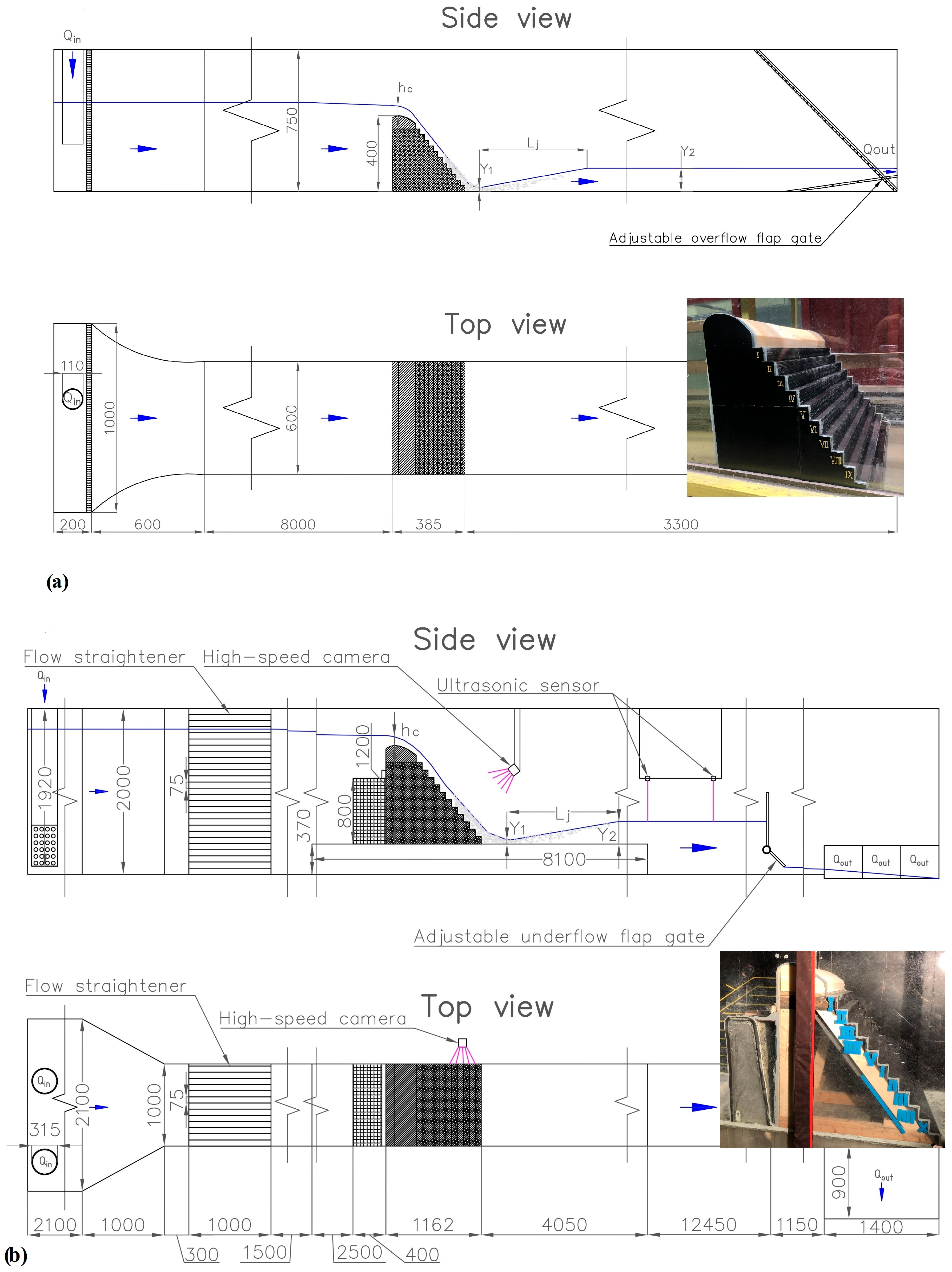
2.1. Experimental Set-Up and Procedure

Experiments were conducted at the Norwegian Hydraulic Laboratory at NTNU using two different scaled stepped spillway models (C-Model and D-Model) in separate flumes, adhering to the Froude similarity law. These models are based on a hypothetical prototype RCC dam with a height of 20 m, corresponding to a slope angle of $\theta =51°$, featuring a vertical water edge and a downstream slope of 1:0.8 (V:H). The prototype consists of 11 steps (N_s), each with a step height h_s of 1.5 m. The scaled models, built to Froude similitude, were constructed in rectangular flumes to achieve the desired skimming flow regime within the limitations of flume size and available discharge. This design mirrors typical stepped spillways on existing gravity dams in the lower height range (Wright & Cameron-Ellis [14] and Chanson H. [15]). The test results were compared with data from the Hinze Dam Stage 3 (Chanson H. [15]) on the Gold Coast in Australia, which has similar slopes and step heights, with a stepped spillway approximately 35 m high. The C-Model, scaled at 1:50 (Figure 2a), was built in a 20-m-long C-flume using horizontal layers of marine plywood, analogous to the RCC construction method, with a crest of extruded polystyrene (XPS). The D-Model, scaled at 1:17 (Figure 2b), was constructed using planks and marine plywood, also with a crest of XPS, and situated in a 25-m-long, 2-m-high, and 1-m-wide D-flume. Originally, the D-Model had a step of approximately 0.37 m located 1.2 m downstream from the toe, but this plateau was extended to 4 m to allow a hydraulic jump to develop undisturbed from the bed level difference. The use of two different scales facilitated the investigation of scale effects. The size of the D-Model closely matches the 1:15 scale recommended by Boes & Hager [16], though slightly smaller due to flume limitations.

A standard ogee crest was designed following USBR (1987) [17] guidelines, with two upstream radii, $R_1=0.5H_0$ and $R_2=0.2H_0$, where $H_0=4.89$m in the prototype, corresponding to a unit discharge of $q_w=24 {\mathrm{m}}^2/\mathrm{s}$. For this design, the downstream curvature is defined by $y=-0.5H_0{\left(x/H_0\right)}^{1.87}$, y is the vertical distance from the top of the weir, and x the horizontal distance. The height of the curved crest is 2 m, resulting in a slope angle of approximately 40° before the first step. Extending the curvature to an angle of $\theta =51°$ would reduce the number of steps, which was not desirable for the research objectives. Flow regulators were used in both channels to minimize turbulence and create a calm water surface with minimal cross-flow in the flumes. An overview of the C-Model and D-Model is summarized in

Table 1. Overview of model and prototype dimensions.

Name	Scale	H (m)	hs (m)	Hf (m)	Bf (m)	Qmax (m3/s)
Prototype	01:01	20	1.5	-	-	-
C-Model	01:50	0.4	0.03	0.75	0.6	0.058
D-Model	01:17	1.2	0.09	2	1	0.51

Note: H = local energy head, H_f = height of flume, B_f = flume width, Q_max = maximum water discharge.

.

Figure 2. Experimental setup for (a) C-flume and (b) D-flume. Flow direction from left to right and dimensions in millimeters (Mikalsen & Thorsen [18]).

Figure 2. Experimental setup for (a) C-flume and (b) D-flume. Flow direction from left to right and dimensions in millimeters (Mikalsen & Thorsen [18]).

The discharge was monitored using a Siemens Sitrans FM MAG 5100 W (München, Germany), an electromagnetic flow sensor mounted on the inlet pipes. The transmitter was a Siemens Sitrans FM MAG 5000, with an accuracy of 0.2% ± 2.5 mm/s. In the D-flume, the downstream sequent depth of the hydraulic jump was measured by two ultrasonic sensors, Microsonic mic + 130/iu/tc (Dortmund, Germany) with a stated accuracy of ±1%. These sensors were positioned in the center of the flume, with an internal distance of 0.8 m between them, and the upstream sensor was placed 4 m from the spillway toe. In the C-flume, the sequent depth of the hydraulic jump was measured manually using a ruler. The ultrasonic sensors measured depths within a specified range, and preliminary experiments were conducted to determine the relevant range of depths for the different discharges used.

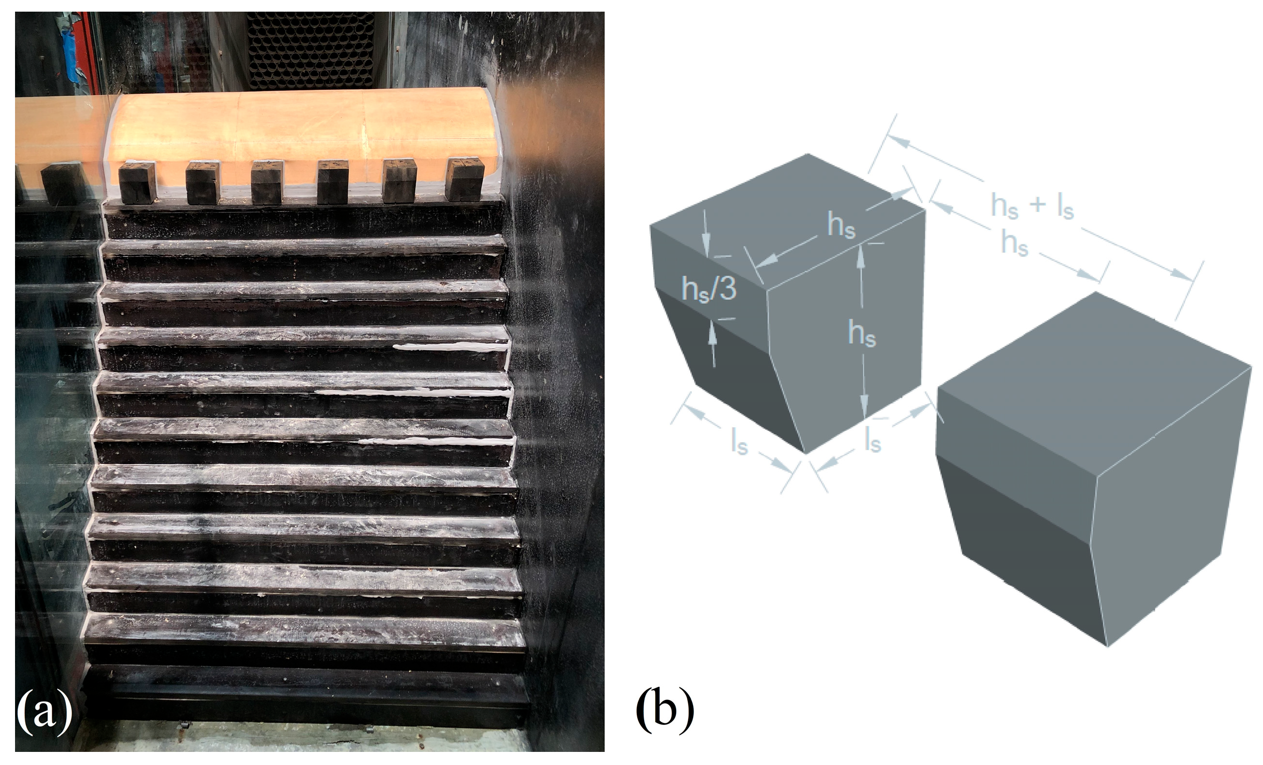
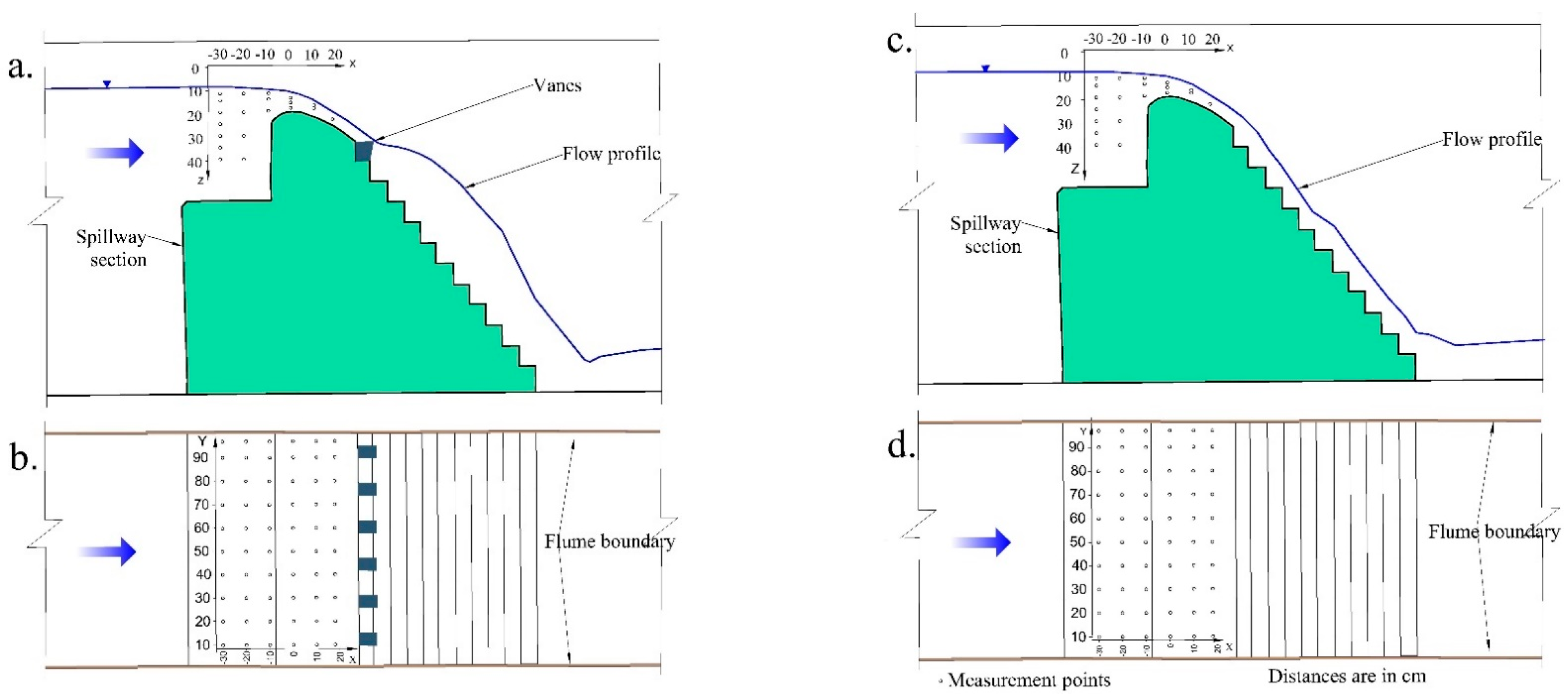
2.2. Crest Splitters

Experiments were conducted both with and without energy-reducing crest splitters. The crest splitters were included to induce additional turbulence near the crest without decreasing the spillway capacity. These crest splitters were inspired by the design criteria outlined by Robert [19], with some modifications to facilitate their implementation in new and existing stepped spillways. The splitters were constructed from wood, as shown in

Table 2. Crest splitters design parameters, prototype scale.

Dimension	Length (m)	Relative Size
Height	1.5	hs
Top length	1.5	hs
Bottom length	1.2	ls
Width	1.2	ls
Gap	1.5	hs
Vertical face	0.5	hs/ 3

and Figure 3. In this study, the experimental results were labeled as “base case” (without splitters) and “with splitters” (with splitters).

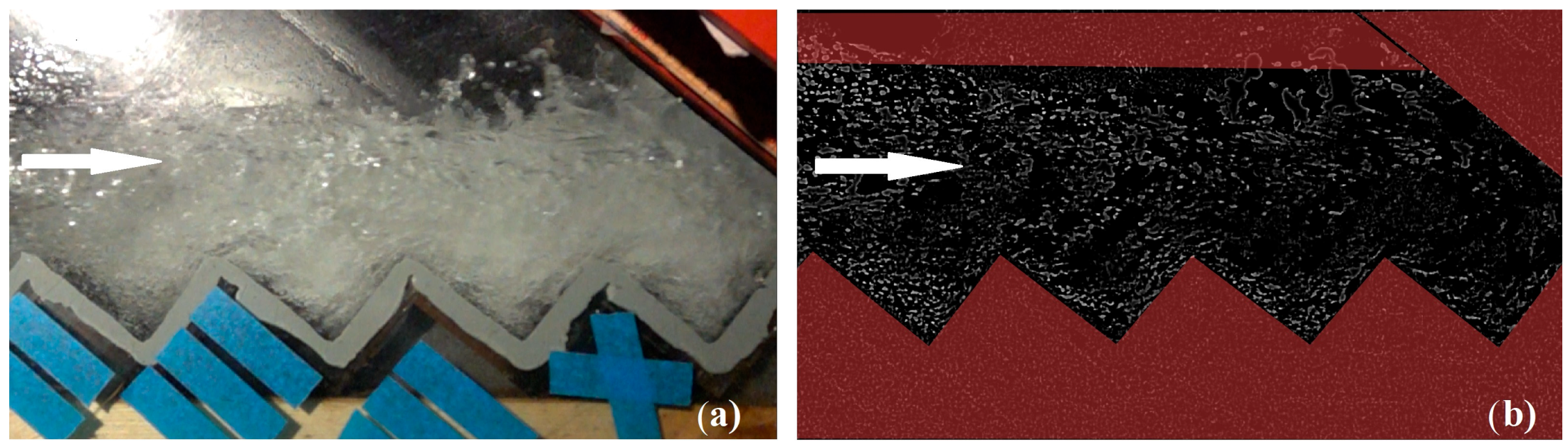
2.3. Procedure for BIV

In this study, flow characteristics and velocity profiles on the steps were developed from side and top video recordings. Videos of bubbles illuminated with intense white light were captured using a SONY DSC-RX0M2G camera with a resolution of 1920 × 1080 pixels, a 16:9 aspect ratio, and a frame rate of 1000 frames per second. The recordings were then analyzed using PIVlab, an open-source toolbox in MATLAB R2023a. Strong white light sources were utilized during the experiments to increase the concentration of air within the flow, which darkened the areas farthest from the flow and made the air bubbles more distinct. Using the classical Particle Image Velocimetry (PIV) technique, PIVlab tracks the tracer particles to obtain the flow velocity field through image processing (William & Stamhuis [20]). There are three stages in BIV analysis: image pre-processing, evaluation, and post-processing. Figure 4 illustrates the result of the pre-processing stage and the consequent improvement in the photograph quality.

The red areas in the photo were then masked, and particle movements in these regions were omitted from the analysis to save processing time. This image evaluation phase leaves only the air bubbles, which the program identifies as white particles on a black background, facilitating frame-to-frame analysis. The results from each particle movement between frames were averaged over 2042 ms, and default settings were used for post-processing. To ensure accurate velocity extraction, a known measured reference length was used for calibration.

2.4. Experiment Parameters

The experiments in the C- and D-flumes were conducted with an initial normalized critical depth of $h_c/h_s=0.8$. The discharge was controlled by manual valves and measured using an electromagnetic flow sensor. All models were run with increased discharges from a depth of $h_c/h_s=0.8$ to approximately $h_c/h_s=3.3$ with intervals of $h_c/h_s=0.1$. This corresponds to prototype unit discharges ranging from $q_w=4 {\mathrm{m}}^2/\mathrm{s}$ to $q_w=34 {\mathrm{m}}^2/\mathrm{s}$.

Table 3. Summary of parameters in experiments.

Model	λf (-)	Q (L/s)	hc/hs (-)	Re (-)	W (-)
C-Model	50	7.2–58	0.6–3.2	1.2 × 104–9.5 × 104	32–62
D-Model	17	61–510	0.6–3.3	6.1 × 104–5.1 × 105	106–179

Note: λ_f = length scale factor in Froude similitude, R_e = Reynolds number, W = Weber number.

shows the range of Reynolds numbers and Weber numbers, along with the range of discharges for the experiments. The Weber number in this study was calculated in the upstream cross-section of the hydraulic jump at the dam toe, as measuring the depth-averaged mixture velocity $\overline{u_m}$ is not possible without intrusive probes. To reduce uncertainty in the results, the experimental program was repeated three times for each of the four models.

Three-component instantaneous flow velocities $(u,v,w)$ on the ogee crest were measured with a Nortek ADV (Bologna, Italy) (10 MHz) device at a sampling frequency of 100 Hz for the D-Model with a discharge of $Q=110 L/s.$ Velocity measurements were recorded for 3 min at each measurement point, resulting in the collection of approximately 18,000 data points per location. This sample size was considered appropriate given the turbulence in the downstream region of the full crest point (Bor [21]). The collected velocity component data were processed and cleaned using the phase-space threshold (PST) filter algorithm, which was employed to remove outliers from the velocity time series based on the physical principle that maximum particle acceleration should not exceed a certain value (Goring & Nikora [22]). In the initial data processing, the ExploreV Pro program was used to discard points with an average correlation below 70% or an SNR below 15 dB. Subsequent data processing and time-averaging of the velocity measurements were performed using MATLAB code, which was developed specifically for ADV data post-processing and consists of several independent functions. In Figure 5, the measurement mesh points are shown both in plan and vertical views: 495 mesh points were used, including 6 profiles in the x-direction and 10 profiles with 5 cm vertical spacing in the y-direction.

3. Experimental Results

3.1. Post-Processing of the Flow Characteristics

Velocity values were measured for a highly aerated flow over a stepped spillway using the BIV method, which employs air bubbles trapped in the flow as tracers. In Figure 6a, velocity vectors from the BIV analysis can be observed at the maximum discharge of the D-Model base case. No free surface aeration occurred in either C-Model or D-Model under maximum discharge conditions; therefore, bubbles were introduced at the first step to serve as BIV tracers. Figure 6a,b illustrate the phenomenon of circulating vortices in the step cavities. In the BIV analysis, the density of vectors does not represent the density of information in the velocity field; rather, the length of the vector represents the magnitude of the velocity.

Figure 7a displays the skimming flow conditions in the stepped spillway models. The point of inception was observed at $L_x/X_s=5$ under the $h_c/h_s=1.2$ flow condition in the D-Model. Figure 7b shows the C-Model under maximum flow conditions. For very low discharges, up to approximately $h_c/h_s=0.6$ in the C-flume and slightly less in the D-flume, the water formed a deflection nappe from the first step, which descended as a free-falling nappe before approaching the spillway further downstream. Figure 7c illustrates the nappe deflecting out from step I and landing on the stepped chute further downstream at step IV. For even smaller discharges, the nappe was observed hitting step VIII/IX.

Figure 8 shows a comparison of the C-Model and D-Models for the transition of flow regimes in base case and splitters configuration experiments under $h_c/h_s=1.2$ flow conditions. It can be observed that the splitters can alter the skimming flow regime at intermediate discharges. For discharges of $h_c/h_s=1.2$ in the D-Model and $h_c/h_s<1.5$ in the C-Model, the splitters caused a water jet to deflect off the spillway, resulting in a free-falling jet that descended to a lower level of the stepped spillway invert.

In addition to this deflecting jet, it is possible to observe air pockets inside the cavities, which reduce the traditional step-cavity circulation of the skimming flow regime, as shown in Figure 9. The regional drowning of the splitters is rather unstable and appears to be influenced by upstream turbulence and transverse flow.

This new flow regime observed at low to intermediate discharges, combined with the splitters’ configuration, exhibits considerable aeration and lacks a distinct pseudo-bottom, resembling a transitional flow regime, although it appears more stable. Figure 10 displays the unstable transitions occurring at flow rates of about ${1.8\le h}_c/h_s\le 2.0$ in the D-flume.

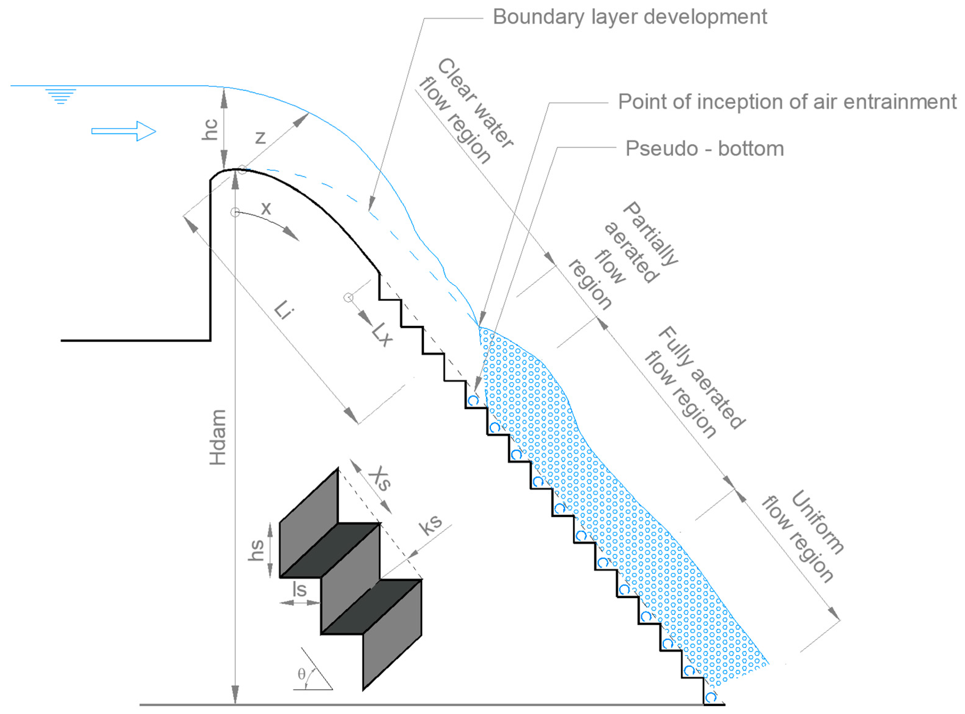
3.2. Inception of Free-Surface Aeration

The classical definition of the inception of free-surface aeration is the point at which the turbulent boundary layer reaches the free surface in stepped chutes (Figure 1). To maintain consistency with the literature, the studies by Hunt & Kadavy [23] and Hunt et al. [24] were used to guide the introduction of the inception of free-surface aeration. In these studies, $L_{i }$ s defined as the downstream distance from the downstream edge of the spillway crest to the point where “white water” first appears across the entire width of the stepped chute’s free surface—in other words, where the turbulent boundary layer reaches the surface. Wood [25] derived an empirical relationship for defining the inception of free-surface aeration $L_{i }$ for smooth chutes, as follows:

$${\displaystyle \frac{L_i}{k_s}}=13.6{\left(sin\theta \right)}^{0.0796}{F}_{\ast }^{0.713}$$

(1)

where $\theta =51.3°$ is the spillway slope for this study; k_s is the step roughness (normal height of the step in this study); $F_{\ast }$ is the roughness Froude number and given as:

$$F_{\ast }={\displaystyle \frac{q_w}{\sqrt{gsin\left(\theta \right)k_s^3}}}$$

(2)

where q_w is the discharge per unit width and g is the gravitational acceleration. Validating with several independent studies, Boes & Hager [16] stated the following free-surface inception point relationships for skimming flow conditions as the point with 0.01% air for slopes of ${26}^0\le \theta \le {55}^0$,

$${\displaystyle \frac{L_i}{k_s}}={\displaystyle \frac{5.90{\left(cos\theta \right)}^{1/5}}{sin\theta }}{F}_{\ast }^{4/5}$$

(3)

In their study, they defined the depth-averaged air concentration at the point of origin as follows:

$${\overline{C}}_i=1.2\times {10}^{-3}\left(240-\theta \right)$$

(4)

where ${\overline{C}}_i$ is the depth-averaged air concentration at the point of inception. Matos [26] determined the point of inception as where the boundary layer reached the free surface and determined that the average value of $C_{meani}\approx 0.2$ for steep slopes.

$${\displaystyle \frac{L_i}{k_s}}=6.289F_{\ast }^{0.734}$$

(5)

$${\overline{C}}_i=0.163F_{\ast }^{0.154}$$

(6)

In this study, the inception of free-surface aeration was determined visually by analyzing digital images for each experiment. The dimensionless inception point distance $L_i/k_s$ was observed with respect to the free-surface inception point $L_i$ and surface roughness for vertical face steps $k_s$. Figure 11 presents a comparison of the experimental measurements with the empirical relationships proposed by Wood [25], Boes & Hager [16] and Matos [26] alongside the prototype data from the Hinze Dam (Chanson H. [15]) used for validation.

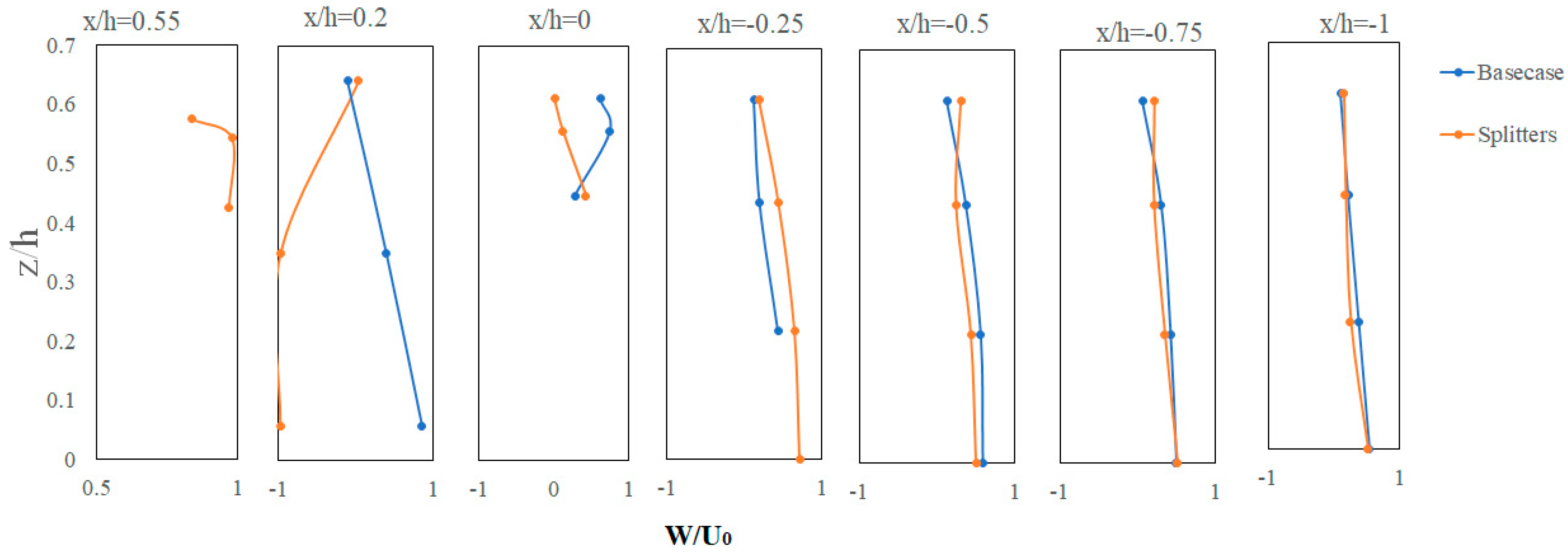
3.3. Velocity Profiles over Step Edges

For flow in both the aerated and non-aerated regions, the velocity distribution is best described by a power law (Chanson H. [1], Amador et al. [27] and Meireles et al. [28]):

$${\displaystyle \frac{u_m\left(z\right)}{u_{90}}}=D{\left({\displaystyle \frac{z}{z_{90}}}\right)}^{1/n}$$

(7)

$${\displaystyle \frac{u\left(z\right)}{u_{FS}}}={\left({\displaystyle \frac{z}{\delta }}\right)}^{1/n}$$

(8)

where ${\displaystyle \frac{u_m\left(z\right)}{u_{90}}}$ is the dimensionless mixture velocity with $u_m\left(z\right)$ being the mixture velocity in the normal distance z over the pseudo-bottom. $u_{90}$ is the mixture flow velocity at the characteristic flow depth $z_{90}$ with the local air concentration of 90%, often defined as the surface of the air–water mixture flow. ${\displaystyle \frac{z}{z_{90} }}$ is the dimensionless mixture flow depth. For non-aerated flows, ${\displaystyle \frac{u_z}{u_{FS}}}$ is the dimensionless velocity, $u_{FS}$ is the free-stream velocity, and $\delta$ is the boundary layer thickness, defined as the normal distance z, where the velocity reached 99% of the maximum value (Zhang & Chanson [3], Kramer [5] and Amador et al. [9]). The coefficients D and n are selected to fit the data obtained from the experiments, with n often exhibiting a wider range of values than D, which is typically set to 1. The coefficient n ranges from 3.0 to 5.4 in the non-aerated zone and from 6.6 to 14 in the aerated region. Some studies have reported for which values of $H_{90}={\displaystyle \frac{z}{z_{90}}}$ the flow follows the power law. Above the boundary layer in both non-aerated and aerated flows, the velocity remains relatively constant up to the surface. An empirical relation between chute slope, normalized discharge, and the power-law coefficient n was proposed by Takahashi & Ohtsu [29] and later utilized by Kramer [5] as follows:

$$n=14{\theta }^{-0.65}{\displaystyle \frac{h_s}{h_c}}\left({\displaystyle \frac{100}{\theta }}{\displaystyle \frac{h_s}{h_c}}-1\right)-0.041\theta +6.27 \mathrm{f}\mathrm{o}\mathrm{r} {19}^{°}\le \theta \le {55}^{°}$$

(9)

where $\theta$ is the angle of the chute slope, h_s is the height of the step, and h_c is the critical depth. Researchers have proposed other models for describing flow velocities over triangular cavities. Kramer [5] combined four different models in his study, creating a multilayered velocity model that corresponded well with measurement data. The number of parameters required for such a model is higher than for simpler models using the power law. The model proposed for the mixing layer by Kramer [5] is as follows:

$${\overline{u}}_{ML}=\left({\overline{u}}_{if}-{\overline{u}}_{min}\right)\left(1+tanh{\displaystyle \frac{z-z_{if}}{L_e}}\right)+{\overline{u}}_{min}, \mathrm{i}\mathrm{f} z<\delta$$

(10)

where ${\overline{u}}_{ML}$ corresponds to the mixing layer velocity, ${\overline{u}}_{if}$ is the velocity at the infection point, ${\overline{u}}_{min}$ is the minimum velocity in the mixing layer, and $L_e$ is the characteristic length scale of the mixing layer. $z_{if }$ denotes the elevation of the inflection point above the pseudo-bottom, under the conditions outlined below::

$${\displaystyle \frac{\overline{u}-{\overline{u}}_{min}}{{\overline{u}}_{FS}-{\overline{u}}_{min}}}=0.5$$

(11)

where $\overline{u}$ is the time-averaged streamwise velocity. In this study, the velocity profiles were calculated from time-averaged BIV measurements without validation. Due to the absence of instrumentation for measuring air concentration, the velocity distribution equation was applied in both the aerated and non-aerated zones. Figure 12 shows a comparison of the theoretical power law velocity distribution with the velocity profiles measured by BIV over step edges at locations $L_x/x_s=4,5,6,7,8,9$ with $h_c/h_s=1.2$ for the D-Model base case.

Figure 13 presents a comparison of velocity profiles measured with BIV at locations $L_x/x_s=5.5$ and $L_x/x_s=6.5$ with $h_c/h_s=1.2$ in the D-Model for both the base case and the splitters configurations.

Figure 14 presents a comparison of surface velocities measured with BIV from a top view at $h_c/h_s=1.2$ and $h_c/h_s=1.6$ in the C-Model and D-Model for the base case configuration. “IP” corresponds to the inception point, or the location where free-surface aeration begins.

3.4. Flow Patterns on Ogee Crest

For each data point, the time-averaged components of the velocity vectors were measured and normalized by the average flow velocity $\left(u_0\right)$. The figures were generated using dimensionless lengths, where h represents the ogee height. The contours of the normalized horizontal velocity components $u/u_0$ and $v/u_0$ are shown in Figure 15 for both the base case and splitters configurations. Figure 16 presents contour plots of $U_{xy}=\sqrt{{\left(\overline{u}/u_0\right)}^2+{\left(\overline{v}/u_0\right)}^2}$, along with horizontal velocity vector plots of $\overline{u}$ and $\overline{v}$ the flow surface, displayed on a horizontal plane with a color scheme for both the base case and splitters configurations.

According to ADV measurements, the normalized vertical velocity vectors $w/u_0$ along to the channel axis are plotted for stream-wise locations $x/h=0.55, 0.2, 0,-0.25,-0.5,-0.75$, and $-1.0$ as presented in Figure 17.

In Figure 17, the normalized vertical one-dimensional profiles $w/u_0$ taken along these streamwise locations are compared for both the base case and splitters configurations. As shown in Figure 17, the profiles become nearly identical after the streamwise location $x/h=-0.25$.

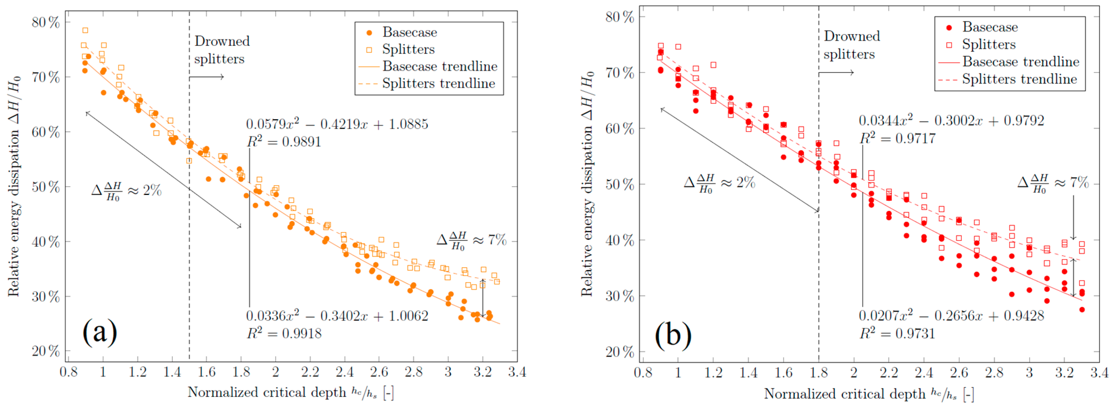
3.5. Energy Dissipation

The energy head in the stepped spillway flow region was examined based on total load measurements. H₀ represents the vertical distance from the point of inception. The energy dissipation rate ΔH was calculated as follows:

$$\mathsf{\Delta }H={\displaystyle \frac{1}{d}}\times {\int }_0^d(H_t-z_0)\times dy$$

(12)

where d is the flow depth, $H_t$ is the total head, and $z_0$ is the step edge elevation above the datum. Experimental data on relative energy dissipation in the C-Model and D-Model, estimated using the hydraulic jump method, are presented in Figure 18a and Figure 18b, respectively.

It was observed that energy dissipation occurred in the boundary layer flow through turbulence and viscosity in the flow region that developed over both stepped spillway models. In the experiments conducted with the D-Model, when $h_c/h_{s }<1.8$, the energy dissipation difference between the base case and the splitters in the stepped spillways was 2%, increasing to 7% when $h_c/h_{s }>1.8.$ The trend is similar in both the base case and splitters flow profiles, as demonstrated by polynomial curve fits with $R^2>0.97$:

$$0.02x^2-0.27x+0.94 \mathrm{f}\mathrm{o}\mathrm{r} \mathrm{B}\mathrm{a}\mathrm{s}\mathrm{e} \mathrm{c}\mathrm{a}\mathrm{s}\mathrm{e}$$

$$0.03x^2-0.3x+0.98 \mathrm{f}\mathrm{o}\mathrm{r} \mathrm{S}\mathrm{p}\mathrm{l}\mathrm{i}\mathrm{t}\mathrm{t}\mathrm{e}\mathrm{r}\mathrm{s}$$

A similar situation was observed in the experiments with the C-Model, but the splitters became submerged at a reduced discharge. More stable measurements with less scattering were observed in the C-Model, with a normalized correlation coefficient of $R^2=0.99$ compared to the D-Model with its polynomial curve:

$$0.03x^2-0.34x+1 \mathrm{f}\mathrm{o}\mathrm{r} \mathrm{B}\mathrm{a}\mathrm{s}\mathrm{e} \mathrm{c}\mathrm{a}\mathrm{s}\mathrm{e}$$

$$0.06x^2-0.42x+1 \mathrm{f}\mathrm{o}\mathrm{r} \mathrm{S}\mathrm{p}\mathrm{l}\mathrm{i}\mathrm{t}\mathrm{t}\mathrm{e}\mathrm{r}\mathrm{s}$$

4. Discussion

4.1. Flow Regimes and Velocity Distribution in the Step Edges

The velocity results from the BIV analysis indicated that the water column consists of a developing boundary layer with an ideal flow region above it. The flow accelerates downstream due to gravitational forces. Regarding the new deflecting nappe flow regime observed at intermediate flow rates (Figure 7a–c), the splitter configuration presents two drawbacks: intense spray and unstable transitions. These issues could potentially be resolved by optimizing the splitter geometry, which warrants further investigation. Another observation in the deflecting nappe regime is that the increase in relative energy dissipation is less substantial than the increase observed in the skimming flow region following the implementation of splitters.

For the profiles over step edges presented in Figure 12 and Figure 13, the best data fit yielded a trendline value of $n=3.6$ with a normalized correlation coefficient of $R^2=0.99$. This value of n is close to that suggested by other studies for similar chute slopes (Kramer [5] and Amador et al. [9]) for the stepped model. It should be noted, however, that these power-law coefficients are calculated from the non-aerated blackwater region. The analytic solution using Equation (9) gives $n=4.7$ which shifts the graph to the right and generally results in larger dimensionless velocities for all values of ${\displaystyle \frac{z}{\delta }}$. The velocity profiles developed with BIV appear to correspond well with established mixing layer theory in the mixing zone. The velocity profiles for the base case from the inner corner of the steps are almost identical to those reported by Sánchez-Juny et al. [4]. There are also similarities between the results of Amador et al. [9] and the mixing layer theory equation proposed by Kramer [5], although minor differences exist, particularly below the pseudo-bottom. At the bottom of the graph, negative streamwise velocity values are observed, with a minimum occurring at approximately $z/\delta \approx -1.$ From this point, the velocities evolve towards positive values, passing through the zero point, which is presumably at the center of the cavity vortex. The velocities seem to decrease after the end of the boundary layer, most likely due to the increasing air concentration in this zone, which reduces the number of bubbles available for tracking by the BIV algorithm.

Above the boundary layer $\delta$, the velocity appears to decrease. This phenomenon was also reported by Sánchez-Juny et al. [4], who suggested that it might be due to insufficient lighting rather than actual flow velocities. However, observations from the present study indicate that the reduction in surface velocities is more likely a consequence of the difficulty in accurately defining the free surface. The probable cause is that PIVlab tracks sporadic droplets in the air above the surface rather than air bubbles within the air–water volume; as a result, the velocity decreases when the upper region of the frames, which includes these sporadic droplets and stationary air, is time-averaged.

The streamwise velocity distribution resulting from the deflecting nappe regime with the splitters configuration exhibits somewhat different characteristics. The greatest negative values are observed at the lowest part of the graphs, and the zero point is positioned further down, indicating that, compared to the base case, the cavity vortex is located closer to the inner corner of the step. This observation aligns closely with the visual observations shown in Figure 8. Due to the free-falling nappe deflecting off the splitters (Figure 7), the graphs are extended upwards.

Surface velocities captured from the top view (Figure 14) exhibit a tendency to oscillate until reaching the inception point, but downstream of this point, the corresponding raw data points show greater stability. This was possibly caused by light glares in the glossy blackwater region. Sánchez-Juny et al. [4] reported much larger differences in velocity magnitude before and after the inception point, attributing these differences to poor lighting; however, no such considerable differences were observed in this study.

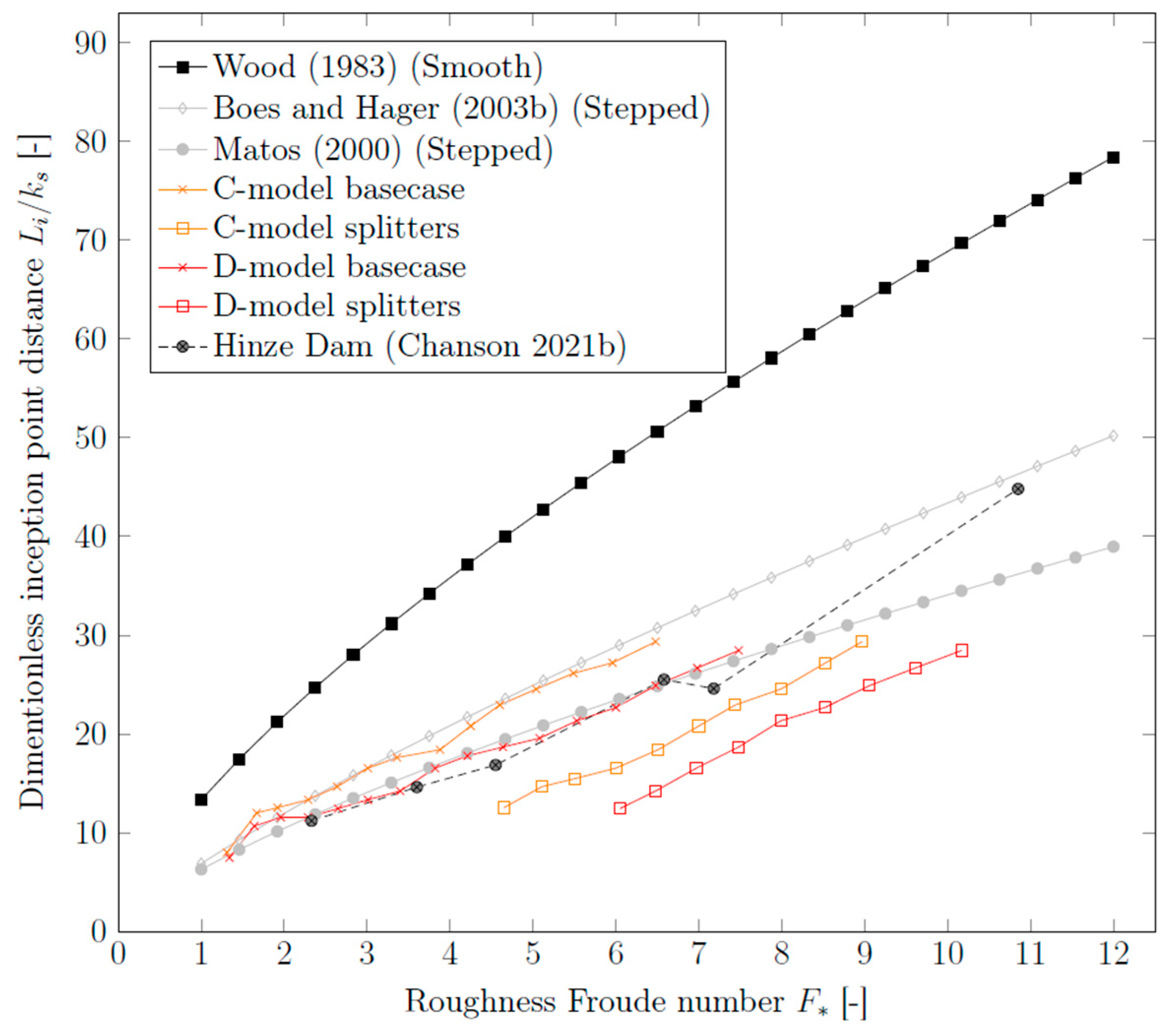
4.2. Length of Inception and Cavitation Potential

The comparison of the point of inception showed relatively good agreement between the C-Model base case and Boes & Hager [16], as well as between D-Model base case and Matos [26] (Figure 11). The prototype data from the Hinze Dam also closely correspond, particularly with the primary D-Model. When the splitters configuration was added to the models, the inception point distance decreased, resulting in a shift of approximately the dimensionless distance $L_i/k_s=10$. This indicates that adding the splitters accelerates the growth of the turbulent boundary layer. The base case hydraulic models correlate well with the established empirical relations for the growth of the turbulent boundary layer toward the water surface and the subsequent free-surface aeration.

Air concentration near the pseudo-bottom is a critical parameter in reducing cavitation. The air concentration at the pseudo-bottom can be calculated using the equation provided by Boes & Hager [16]:

$$C_b\left(x_i\right)=0.015x_i^{\sqrt{tan\theta }/2} \mathrm{for} {26}^{°}\le \theta \le {55}^{°}$$

(13)

where $x_i=(x-L_i)/z_{m,i}$ is the non-dimensional distance from the inception point, x is the longitudinal streamwise distance from the crest of the spillway, and $z_{mi}$ is the air–water mixture depth at the point of inception. At the point of inception, the air concentration at the pseudo-bottom $C_{bi}=0.01$ and the depth-averaged air concentration ${\overline{C}}_i=0.226$ with a slope of $\theta =51°$ result from the increasing non-linear relationship between water depth and air concentration (as derived from Equations (4) and (13)).

Frizell et al. [30] made the following recommendation regarding cavitation in their research on stepped spillways within a closed system with reduced ambient pressure:

$${\sigma }_c>{\sigma }_{cr}=4f$$

(14)

where ${\sigma }_c$ is the cavitation index and ${\sigma }_{cr}$ is the critical cavitation index. Boes & Hager [16] provide the friction factor f, including sidewall correction, as follows:

$${\displaystyle \frac{1}{\sqrt{f}}}={\displaystyle \frac{1}{\sqrt{0.5-0.42sin\left(2\theta \right)}}}\left[1-0.25log\left({\displaystyle \frac{h_{s}cos\left(\theta \right)}{D_{h,w,u}}}\right)\right]$$

(15)

where $D_{h,w,u}$ corresponds to the equivalent clear water hydraulic diameter in the quasi-uniform zone of the flow and $h_s$ is the height of step. The cavitation index is defined as follows:

$${\sigma }_c={\displaystyle \frac{P_0-P_v}{\frac{1}{2}{\rho }_w{u}_0^2}}$$

(16)

where P₀ is the pressure at flow surface, P_v, is the vapor pressure, ${\rho }_w$ is the water density and u₀ is the mean velocity. According to the cavitation control for the experiments, cavitation was determined at a value of 3.3, corresponding to a unit discharge of $q_w=34.5 {\mathrm{m}}^2/\mathrm{s}$ and a normalized critical depth of $h_c/h_s$. The control was conducted for a unit width at the position of $L_x/x_s=11$, meaning that the hydraulic radius was $R_h=z_w=z$ due to the non-aerated flow. The velocity at this position was not measured directly for this discharge but was assumed to be $\sqrt{\eta }{u}_1=20 \mathrm{m}/\mathrm{s}$ based on the energy loss factor reported by André [31], where η = 1.15. $u_1$ is the mean velocity in the upstream cross-section of the hydraulic jump. The critical cavitation index was calculated as ${\sigma }_{cr}=0.244$ for this position. $D_{h,w,u}$ was assumed to be 4R_h despite the uniform flow not being fully developed. This critical cavitation index is less than the cavitation index ${\sigma }_c=0.487$, indicating that cavitation is not expected. The calculations were performed with a vapor pressure $P_v=2.4 \mathrm{k}{\mathrm{P}}_{\mathrm{a}},$ a water density ${\rho }_w=1000 \mathrm{k}\mathrm{g}/{\mathrm{m}}^3$, and a reference pressure P₀ as the atmospheric pressure. Further calculations show that the critical velocity for inducing cavitation in the prototype is approximately 28 m/s, significantly higher than the value proposed by Boes & Hager [16].

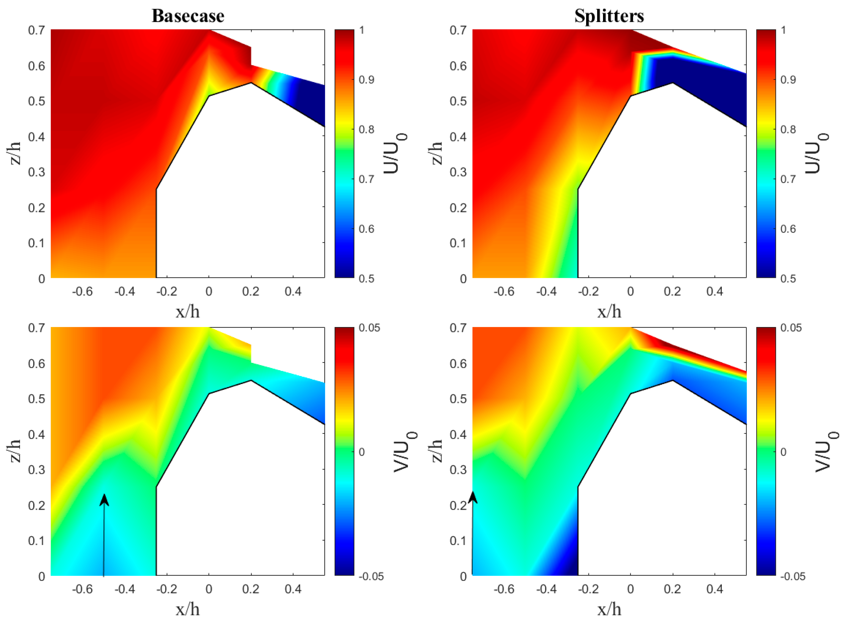
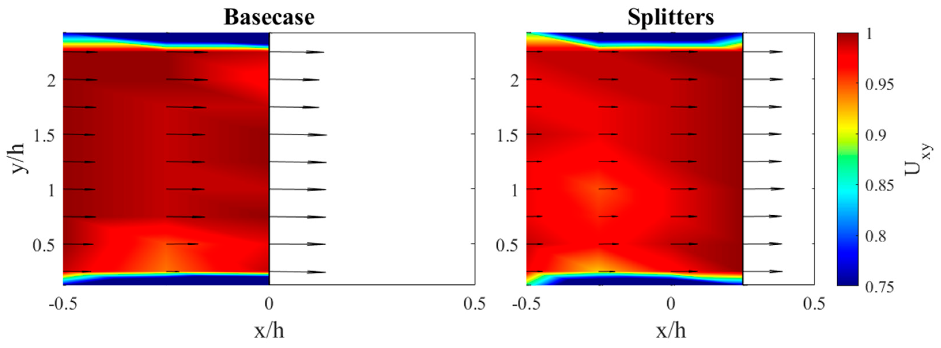
4.3. Effect of Crest Splitters on Velocity Patterns above the Ogee Crest and Energy Dissipation

With reference to Figure 15, the normalized horizontal velocity components (u, v) and the vertical velocity component (w) obtained from ADV measurements show that as the flow approaches the ogee crest, the average flow velocity increases due to the decreasing cross-sectional area, reaching a maximum at the crest. After passing the peak, the water velocity decreases on the downstream side. In general, it has been observed that the velocity vectors (u and w) play a dominant role in both the base case and splitter experiments. The splitters slightly increased the water depth on the upstream side, which appears to cause a further decrease in water velocity and a corresponding reduction in energy. Additionally, it was observed that the splitters somewhat reduced the velocity, and therefore the energy, in the upstream part of the ogee crest and towards the downstream flow. In the splitter experiments, u decreased by 65% when the element was slightly above the ogee crest. Normalized horizontal velocities indicate that the zone of positive average vertical velocity $v/u_0$ increases toward the top of the ogee crest, while negative velocities occur toward the bottom. The splitters caused the velocities to shift upstream to $x/h=0.5$ from the upstream side of the ogee crest, leading to a decrease in velocities both upstream and downstream of the ogee crest.

In Figure 17, changes in the vertical velocity vector direction $w/u_0$ can be seen after the flow passes over the ogee crest in the splitter configuration. The splitters were observed to increase water depth upstream of the crest, which slightly reduces velocity and, consequently, energy both upstream of the crest and toward the rear of the flow. In the upstream part of the flow, the velocity vectors in the base case and with splitters move in opposite directions. However, beyond the streamwise location $\left(x/h=-0.25\right)$, the profiles become almost identical.

Another advantage of the stepped spillway is the continuous energy dissipation along the spillway chute, with splitters contributing to a 7% increase in relative energy dissipation. This results in a large area over which energy is dissipated, reducing the stresses on the concrete and bedrock. In the C-Model, less turbulence, higher relative surface tension, and proportionally larger air bubbles could all contribute to reduced aeration and, to some extent, lower energy dissipation. As shown in Figure 18, a semi-linear decrease in normalized specific energy is observed, consistent with previous studies Zhang & Chanson [3], Hunt et al. [24] and Meireles et al. [28].

4.4. Scale Effects and Uncertainty

Scale effects are inevitable when downscaling highly turbulent two-phase flows. As anticipated, reduced energy dissipation and lower aeration efficiency were observed in the C-Model. In terms of flow transitions, the deflecting water jet over the splitters was observed across a wider range of normalized critical depths in the D-flume. The influence of the Weber number may explain why surface tension forces are more pronounced in the smaller C-Model, causing greater resistance for the nappe to deflect from the main flow.

The air bubbles in the two different scale models were observed to be of similar size, leading to proportionally larger and fewer bubbles in the C-Model relative to the prototype it represents. One practical issue arising from this situation is that the BIV algorithm had fewer bubbles to track, making the C-Model less suitable for BIV analysis.

The relative energy dissipation in the different scale models diverged more significantly at larger dimensionless discharges, with substantial deviations observed at design discharges. At these discharges, the flow in the stepped spillway is not aerated, as seen for $h_c/h_s=3.3$ in Figure 7, indicating that the issue is not related to the two-phase characteristics in the spillway. However, the hydraulic jump at the dam toe is highly turbulent and aerated, making it subject to drastic scale effects, which could explain the deviation in energy dissipation across models at higher flow rates.

While the C-Model appears unsuitable for studying two-phase flow, the two different scale models exhibited very similar changes in relative energy dissipation from the base case to the splitter configuration, supporting the findings from the primary D-Model.

When working with video recordings and BIV analysis, distortion can occur due to the deformation of angles and distances in images caused by the camera lens and perspective. Another issue is the suitability of air bubbles as tracers, given the upward vertical velocity component of the bubbles. Sánchez-Juny et al. [4], who conducted similar experiments, concluded that air bubbles can be used as tracers but did not seem to address this aspect in detail. The findings of lower velocities in dark regions are consistent with those reported by Sánchez-Juny et al. [4]. A possible approach to quantifying the effects of rising velocity, lighting conditions, wall effects, and varying distances to the traced bubbles is to conduct parallel experiments using PIV with seeding particles and a laser-illuminated sheet, as demonstrated by Amador et al. [9]. Using video recordings with 1000 FPS was found to be sufficient for the use of PIVlab. Sánchez-Juny et al. [4] successfully used PIVlab with 400 FPS, suggesting the possibility of reducing the frame rate in this study, thereby saving processing time.

5. Conclusions

This study focused on practical, cost-effective, and feasible measures to improve energy dissipation in stepped spillways using the BIV technique. To investigate scale effects, laboratory tests were conducted with two different scale models, 1:50 and 1:17, while prototype data and a literature review were used to guide the analysis. The following conclusions can be drawn from this research:

−

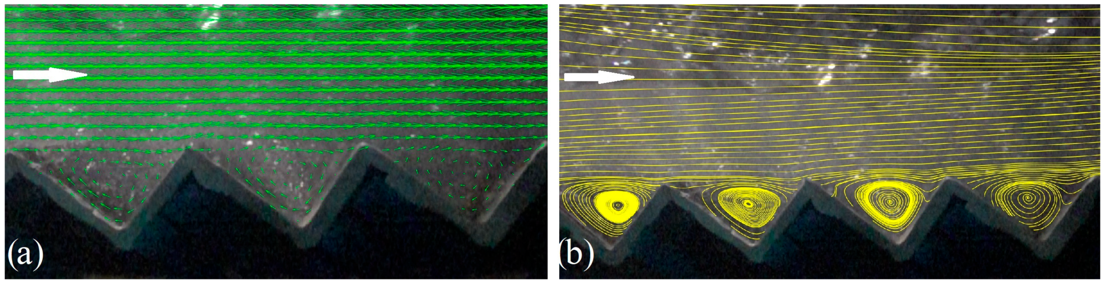
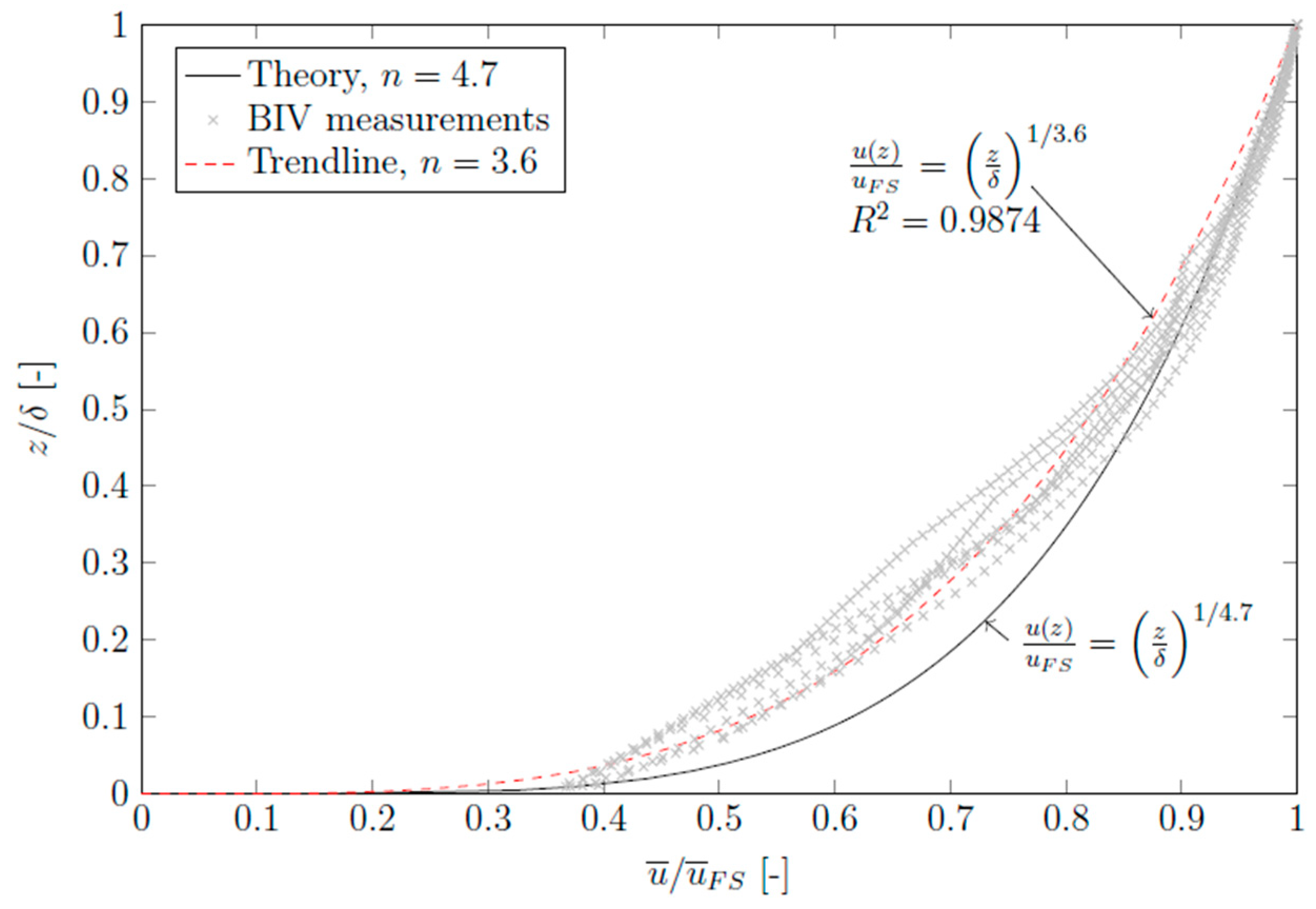
In the experiments, it was observed that the flow region developed in shear flow consists of a turbulent boundary layer, with ideal fluid flow above it. A rapidly changing flow movement was observed along the steps. Bernoulli’s principle was used to calculate the energy distribution, assuming that the flow moved in the downward direction.

−

The splitters were found to increase relative energy dissipation by 7%. In addition to enhancing energy dissipation, the splitters reduced the length of inception to $L_i/k_s$ = 10, thereby lowering the potential for subsequent cavitation. This resulted in an increase in the maximum allowable unit discharge. Consequently, crest splitters can be considered a practical, viable, and cost-effective measure to improve energy dissipation in stepped spillways, applicable to both existing dams and new projects.

−

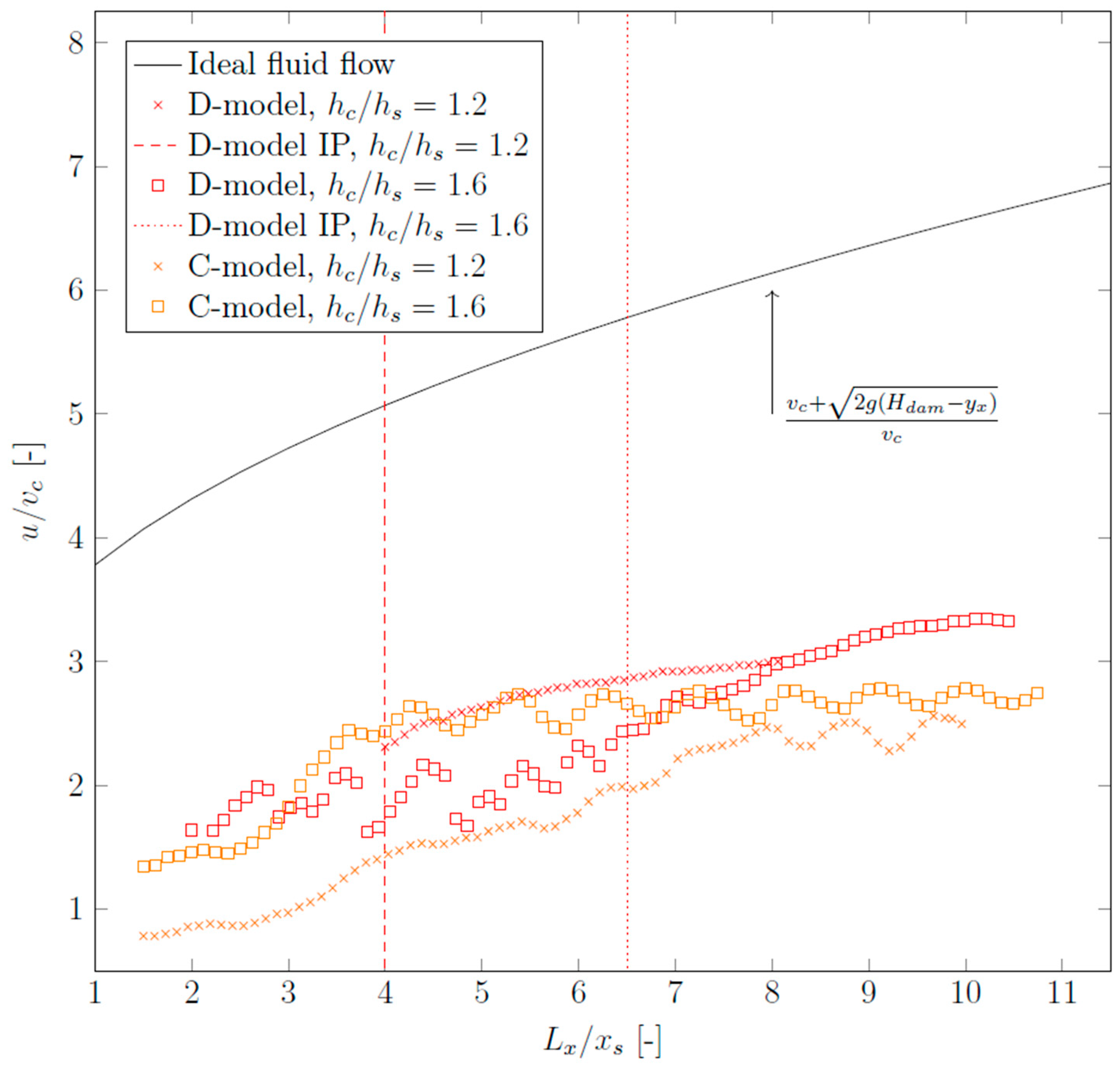
In the experiment with the splitter, the horizontal velocity vector u around the ogee crest showed a significant decrease. Additionally, the vertical velocity vector v contributed to turbulence by changing direction, resulting in decreased average velocities in front of and behind the ogee crest, thereby reducing energy on the downstream side of the spillway.

−

BIV was found to be a straightforward and highly effective technique for accurately measuring and determining flow characteristics in aerated flow conditions, likely the best practice for such applications. BIV enables the collection of large quantities of high-quality data with standard camera equipment, allowing for the extraction of detailed information and the production of dense plots without the need for commercial software or extensive processing capabilities.

−

The scale effects observed in this study align well with established theory. Severe scale effects were noted in the air–water flow in the smaller-scaled model, underscoring the importance of using a larger scale to accurately study highly turbulent two-phase flow conditions. The findings closely correspond to established theory regarding the valid length scales for studying highly turbulent two-phase flow under Froude similitude.

−

While the smaller C-Model appears unfit for the study of two-phase flow, the change in relative energy dissipation from the base case to the splitter configuration is nearly identical for the two different scale models, supporting the findings in the primary D-Model.

References

1. Chanson, H. Hydraulics of Stepped Chutes and Spillways; Balkema Publ: Lisse, The Netherlands, 2001; ISBN 9058093522. [Google Scholar]
2. Kokpinar, M.A. Flow over a stepped chute with and without macro-roughness elements. Can. J. Civ. Eng. 2004, 31, 880–891. [Google Scholar] [CrossRef]
3. Zhang, G.; Chanson, H. Application of local optical flow methods to high-velocity free-surface flows: Validation and application to stepped chutes. Exp. Therm. Fluid Sci. 2018, 90, 186–199, ISSN 0894-1777. [Google Scholar] [CrossRef]
4. Sánchez-Juny, M.; Estrella, S.; Matos, J.; Bladé, E.; Martínez-Gomariz, E.; Bonet Gil, E. Velocity Measurements in Highly Aerated Flow on a Stepped. Water 2022, 14, 2587. [Google Scholar] [CrossRef]
5. Kramer, M. Velocities and Turbulent Stresses of Free-Surface Skimming Flows over Triangular Cavities. J. Hydraul. Eng. 2023, 149, 04023012. [Google Scholar] [CrossRef]
6. Rajaratnam, N. An experimental study of air entrainment characteristics of the hydraulic jump. J. Inst. Eng. 1962, 42, 247–273. [Google Scholar]
7. Murillo, R.E. Experimental Study of the Development Flow Region On Stepped Chutes. Ph.D. Thesis, University of Manitoba, Winnipeg, MB, Canada, 2006. [Google Scholar]
8. Ohtsu, I.; Yasuda, Y. Characteristics of flow conditions on stepped channels. In Proceedings of the 27th IAHR Congress, San Francisco, VA, USA, 10–15 August 1997; pp. 583–588. [Google Scholar]
9. Amador, A.; Sánchez-Juny, M.; Dolz, J. Characterization of the Nonaerated Flow Region in a Stepped Spillway by PIV. ASME J. Fluids Eng. 2006, 128, 1266–1273. [Google Scholar] [CrossRef]
10. Bung, D.; Valero, D. Optical flow estimation in aerated flows. J. Hydraul. Res. 2016, 54, 575–580. [Google Scholar] [CrossRef]
11. Kramer, M.; Chanson, H. Optical flow estimations in aerated spillway flows: Filtering and discussion on sampling parameters. Exp. Therm. Fluid Sci. 2019, 103, 318–328. [Google Scholar] [CrossRef]
12. Lopes, P.; Leandro, J.; Carvalho, R.; Daniel, D. Alternating skimming flow over a stepped spillway. Environ. Fluid Mech. 2017, 17, 303–322. [Google Scholar] [CrossRef]
13. Leandro, J.; Bung, D.; Carvalho, R. Measuring void fraction and velocity fields of a stepped spillway for skimming flow using non-intrusive methods. Exp. Fluids 2014, 55, 1732. [Google Scholar] [CrossRef]
14. Wright, H.C.; Cameron-Ellis, D.G. Energy dissipation provisions for stepped spillways: Are additional measures necessary? A southern african perspective. In Proceedings of the SANCOLD Annual Conference 2018, Pretoria, South Africa, 3–7 November 2018. [Google Scholar]
15. Chanson, H. Energy dissipation on stepped spillways and hydraulic challenges—Prototype and laboratory experiences. J. Hydrodyn. 2022, 34, 52–62. [Google Scholar] [CrossRef]
16. Boes, R.M.; Hager, W.H. Two-Phase Flow Characteristics of Stepped Spillways. J. Hydraul. Eng. 2003, 129, 661–670. [Google Scholar] [CrossRef]
17. USBR Design of Small Dams. Water Resources Technical Publication, third edition. 1987. Available online: https://www.osti.gov/biblio/29108 (accessed on 19 August 2024).
18. Mikalsen, L.; Thorsen, K. Improved Energy Dissipation in Stepped Spillways—Hydraulic Model Study Applying Bubble Image Velocimetry. Master’s Thesis, NTNU, Trondheim, Norway, 2023. [Google Scholar]
19. Robert, D. The dissipating of the energy of a flood passing over a high dam. Civ. Eng. = Siviele Ingenieurswese 1943, 1943, 48–92. [Google Scholar]
20. William, T.; Stamhuis, E. PIVlab—Towards User-friendly. Affordable and Accurate Digital Particle Image Velocimetry in MATLAB. J. Open Res. Softw. 2014, 2, 30. [Google Scholar] [CrossRef]
21. Bor, A. Experimental investigation of 90° intake flow patterns with and without submerged vanes under sediment feeding conditions. Can. J. Civ. Eng. 2022, 49, 452–463. [Google Scholar] [CrossRef]
22. Goring, D.G.; Nikora, V.I. Despiking acoustic doppler velocimeter data. J. Hydraul. Eng. 2002, 128, 117–126. [Google Scholar] [CrossRef]
23. Hunt, S.; Kadavy, K. Inception Point for Embankment Dam Stepped Spillways. J. Hydraul. Eng. 2012, 139, 60–64. [Google Scholar] [CrossRef]
24. Hunt, S.L.; Kadavy, K.C.; Hanson, G.J. Simplistic Design Methods for Moderate-Sloped Stepped Chutes. J. Hydraul. Eng. 2014, 140, 04014062. [Google Scholar] [CrossRef]
25. Wood, I. Uniform Region of Self—Aerated Flow. J. Hydraul. Eng. 1983, 109, 447–461. [Google Scholar] [CrossRef]
26. Matos, J. Hydraulic design of stepped spillways over RCC dams. In Hydraulics of Stepped Spillways; Minor, E.H., Hager, W., Eds.; CRC Press: London, UK, 2000; ISBN 9781003078609. [Google Scholar]
27. Amador, A.; Sánchez-Juny, M.; Dolz, J. Developing Flow Region and Pressure Fluctuations on Steeply Sloping Stepped Spillways. J. Hydraul. Eng. 2009, 135, 1092–1100. [Google Scholar] [CrossRef]
28. Meireles, I.; Renna, F.; Matos, J.; Bombardelli, F. Skimming, Nonaerated Flow on Stepped Spillways over Roller Compacted Concrete Dams. J. Hydraul. Eng. 2012, 138, 10. [Google Scholar] [CrossRef]
29. Takahashi, M.; Ohtsu, I. Aerated flow characteristics of skimming flow over stepped chutes. J. Hydraul. Res. 2012, 50, 427–434. [Google Scholar] [CrossRef]
30. Frizell, K.; Renna, F.; Matos, J. Cavitation Potential of Flow on Stepped Spillways. J. Hydraul. Eng. 2015, 141, 630–636. [Google Scholar] [CrossRef]
31. André, S. High Velocity Aerated Flow on Stepped Chutes with Macro-Roughness Elements. Ph.D. Thesis, EPFL, Lausanne, Switzerland, 2004. [Google Scholar] [CrossRef]
Figure 1. Definition sketch of stepped spillways in skimming flow conditions.
Water 16 02432 g001
Figure 3. Crest splitters positioning: (a) downstream face of the D-Model with crest splitters and (b) design of splitters (Mikalsen & Thorsen [18]).
Water 16 02432 g003
Figure 4. One representative frame from the video recordings before and after pre-processing and masking in PIVlab—flow direction from left to right: (a) original frame; (b) pre-processed and masked frame (The arrow indicates the direction of flow) (Mikalsen & Thorsen [18]).
Water 16 02432 g004
Figure 5. The measurement velocity grids in (a) base case cross-section and (b) base case plan, with (c) with splitters cross-section and (d) with splitters plan (units are in centimeters).
Water 16 02432 g005
Figure 6. (a) Velocity vectors after post-processing; (b) streamlines in D-Model obtained from BIV analysis (flow direction from left to right).
Water 16 02432 g006
Figure 7. (a) Skimming flow for D-Model base case h c / h s = 1.2 ; (b) skimming flow for C-Model splitters h c / h s = 3.3 ; (c) a nappe is formed for very low discharges, C-Model base case h c / h s = 0.6 . (Both of the models’ steps are labelled with Roman symbols).
Water 16 02432 g007
Figure 8. Comparison of flow regimes in the (a) D-Model base case (b) D-Model splitters (c) C-Model base case (d) C-Model splitters, at the same normalized critical depth h c / h s = 1.2 . (Both of the models’ steps are labelled with Roman symbols).
Water 16 02432 g008
Figure 9. Comparison of streamlines obtained from BIV analysis of (a) base case and (b) splitters configuration in D-Model h c / h s = 1.2 and 7 < L x / x s < 8 flow direction from left to right.
Water 16 02432 g009
Figure 10. Video frames displaying unstable transition from (a) a skimming regime to a deflecting nappe regime and (b) a deflecting nappe regime to a skimming regime over approximately 10 s, h c / h s = 1.8 . (Both of the models’ steps are labelled with Roman symbols).
Water 16 02432 g010
Figure 11. Comparison of experimental data, prototype data, and empirical relations for the location of the inception point (Chanson H. [15], Boes & Hager [16], Wood [25] and Matos [26]).
Water 16 02432 g011
Figure 12. Dimensionless velocity profiles measured with BIV over step edges in D-Model base case compared with power-law approach h c / h s = 1.2 ,   z < δ and L x / x s = 4 , 5 , 6 , 7 , 8 , 9 .
Water 16 02432 g012
Figure 13. Velocity profiles in the D-Model measured with BIV compared with mixing layer theory h c / h s = 1.2 , z < δ , L x / x s = 5.5 and L x / x s = 6.5 .
Water 16 02432 g013
Figure 14. Surface velocities in the C-Model and D-Model base case measured with BIV from top-view compared with ideal fluid flow.
Water 16 02432 g014
Figure 15. Contour plots of the normalized horizontal velocities u / u 0 and v / u 0   for the D-Model.
Water 16 02432 g015
Figure 16. Non-dimensional time-averaged velocity magnitude Uxy (–) presented as color scheme for horizontal planes at water surface for the D-Model.
Water 16 02432 g016
Figure 17. Comparison of normalized vertical w / u 0 one-dimensional profiles for stream-wise locations x / h = 0.55 ,   0.2 ,   0 , 0.25 , 0.5 , 0.75 , and 1.0 in base case and splitters cases for the D-Model.
Water 16 02432 g017
Figure 18. Experimental data of relative energy dissipation compared to normalized critical depth in the (a) C-Model and (b) D-Model.
Water 16 02432 g018