Multivariate Geostatistics for Mapping of Transmissivity and Uncertainty in Karst Aquifers

Abstract

Due to their complex morphology, karst terrains are particularly more fragile and vulnerable to environmental damage compared to most natural systems. Their hydraulic properties, such as their transmissivity (T) and spatial variability, can be relevant for understanding groundwater flow and, consequently, for the sustainable management of water resources. The application of geostatistical methods allows for spatial interpolation and mapping based on observations combined with uncertainty quantification. Direct measurements of T are typically scarce, while those of the specific capacity (S_c) are more frequent. We established a linear and spatial relationship between the logarithms of T and S_c measured in 174 wells in a semi-arid karst region in northeastern Brazil. These relationships were used to construct a cross-variogram, whose Linear Model of Coregionalization proved valid. The values and the cross-variogram of logT and logS_c were used to generate interpolations over 2554 values of logS_c, which did not spatially coincide with logT. We used ordinary co-kriging (CO-OK) and conditional sequential Gaussian co-simulation (CO-SGS) to generate the interpolations. The cross-variogram of logT and logS_c, when considering 174 wells, was isotropic with an exponential structure, a nugget effect of approximately 20% of the sill, and a range of 5 km. Cross-validation indicated an optimal number of 10 neighboring wells used in CO-OK, and we used 500 stochastic realizations in CO-SGS, which were then used to generate maps of logT estimates, deviations derived from the interpolations, and probabilistic scenarios. The resulting transmissivity maps are relevant for the design of groundwater management strategies, including stochastic approaches where the transmissivity realizations can be used to parameterize multiple executions of numerical flow models.

1. Introduction

Karst aquifers represent a significant portion of groundwater reservoirs, serving approximately 9% of the world’s population [1]. Due to their facies, structural, and chemical characteristics, these reservoirs exhibit high heterogeneity in the spatial distribution of their hydraulic parameters [2]. Among the most relevant parameters, aquifer transmissivity (T [L²T⁻¹]) stands out due to its classic conception in regional hydrogeology and broad application in pumping tests. Additional parameters include the hydraulic conductivity (K [LT⁻¹]), storage coefficient (S [-]), and specific capacity (S_c [L²T⁻¹]). Except for estimates of S, which are more complex to acquire, all of these parameters can be obtained through single-well tests, such as slug tests, drawdown tests, and recovery tests [3,4,5]. The hydraulic properties of karst aquifers are often reflected in the surface morphology and patterns of internal heterogeneities. For example, areas with higher transmissivity tend to exhibit a greater number of sinkholes. However, in Precambrian karst aquifers, the porosity and groundwater flow patterns are conditioned by the presence of brittle structures such as faults, fractures, and structural lineaments. In this heterogeneous environment, most field observations indicate that T values calculated from S_c data using analytical solutions are consistent with those obtained through pumping tests. Therefore, many hydrogeologists, due to the ease of measuring S_c, have sought to use log–log equations to arrive at estimates of T [6,7,8,9,10,11,12]. Geostatistical methods are widely used in the spatialization of hydrogeological parameters and in the assessment of uncertainties attributed to interpolations. However, a small number of samples can negatively impact the accuracy of the geostatistical model. This problem can be mitigated by using multivariate geostatistical models, such as ordinary co-kriging (CO-OK) and conditional sequential Gaussian co-simulation (CO-SGS) [13]. For example, based on the experience that T is strongly correlated with S_c, it is possible to increase the representativeness of T estimates through measurements of S_c [14,15].

The application of co-kriging is recommended when the sample density of the secondary variable is higher than that of the primary variable [16]. For this, certain assumptions must be observed, such as the existence of a strong linear and spatial correlation between the variables. The linear correlation between T (primary variable) and S_c (secondary variable) is evaluated through a linear fit, allowing for the calculation of the coefficient of determination and identifying the uncertainties associated with the regression. Structural correlation is determined using cross-variograms, which require a valid Linear Model of Coregionalization (LMC).

Existing examples of strongly correlated hydrogeological variables and respective applications of CO-OK in the literature include the combination of hydrostratigraphic data with ground-penetrating radar for estimating hydraulic conductivity [17], or the delineation of heavy metal plumes based on soil sample analysis for different but correlated physical and chemical parameters [18]. CO-OK is also convenient for heterogeneous spatial distributions of samples when compared to simple co-kriging or universal kriging, which would require a priori specification of means or spatial trend surface characteristics [16]. To allow for a possible global trend across the entire dataset, we used CO-OK here based on weights within moving windows over neighboring data [19].

CO-SGS is a multivariate extension of conditional sequential Gaussian simulation (SGS). In this method, estimates are made similarly to CO-OK [20]. In CO-SGS, it is essential to observe a linear and structural correlation between the analyzed data sets. Variables are transformed to follow a Gaussian distribution in order to generate a specific number of random realizations that respect the estimated covariances between the variables. These realizations can be used to propagate uncertainty to subsequent results, such as numerically simulated groundwater levels, using the Monte Carlo methodology [21]. Despite the benefits, the adoption of stochastic simulation approaches remains notably restricted, especially regarding hydraulic parameters in karst aquifers [22].

The study area was in the central portion of the State of Bahia, Brazil, within the Chapada Diamantina mountain range near the city of Irecê. For this study, only the domain of carbonate rocks known as the Una Group was considered, specifically the Salitre Formation. The aquifer associated with the Salitre Formation is called the Salitre Karst Aquifer (SKA), which covers an area of approximately 20,000 km² [11], where agriculture is the main economic activity [23]. The investigated area included the São Francisco River, which is locally present in the western part of the SKA, and three intermittent rivers called Verde, Jacaré, and Paraguaçu. Due to the scarcity of surface water, human activities such as agriculture and industry primarily rely on groundwater. Therefore, it is necessary to understand the hydrodynamic aspects related to the SKA for a better estimation of this aquifer’s potentialities.

Previous studies have spatialized S_c and T data in the SKA [11] using deterministic models (e.g., inverse distance weighting). Geospatial models have only been applied to the southern portion of the SKA, employing robust interpolation techniques such as ordinary kriging and conditional sequential Gaussian simulation [12]. Other studies have also contributed to the hydrogeological understanding of the Salitre Karst Aquifer (SKA) from hydrodynamic and hydrogeochemical perspectives in recent years [24,25,26].

This study aims to map the values of the hydraulic transmissivity and their uncertainties in entire the Salitre Karst Aquifer (SKA) using multivariate geostatistical methods, including co-kriging and stochastic co-simulations. This represents a methodological and geographical extension compared to [12]. We employed ordinary co-kriging and conditional stochastic co-simulation to produce Optimal Unbiased Linear Estimates (BLUE) and multiple realizations of transmissivity maps, respectively. The mapping of the spatial variability and uncertainty of T in the SKA will significantly contribute to understanding groundwater flow patterns and identifying areas with high potential for well drilling. Additionally, this information will be valuable for artificial recharge projects, numerical modeling, and water resource management in the region.

2. Materials and Methods

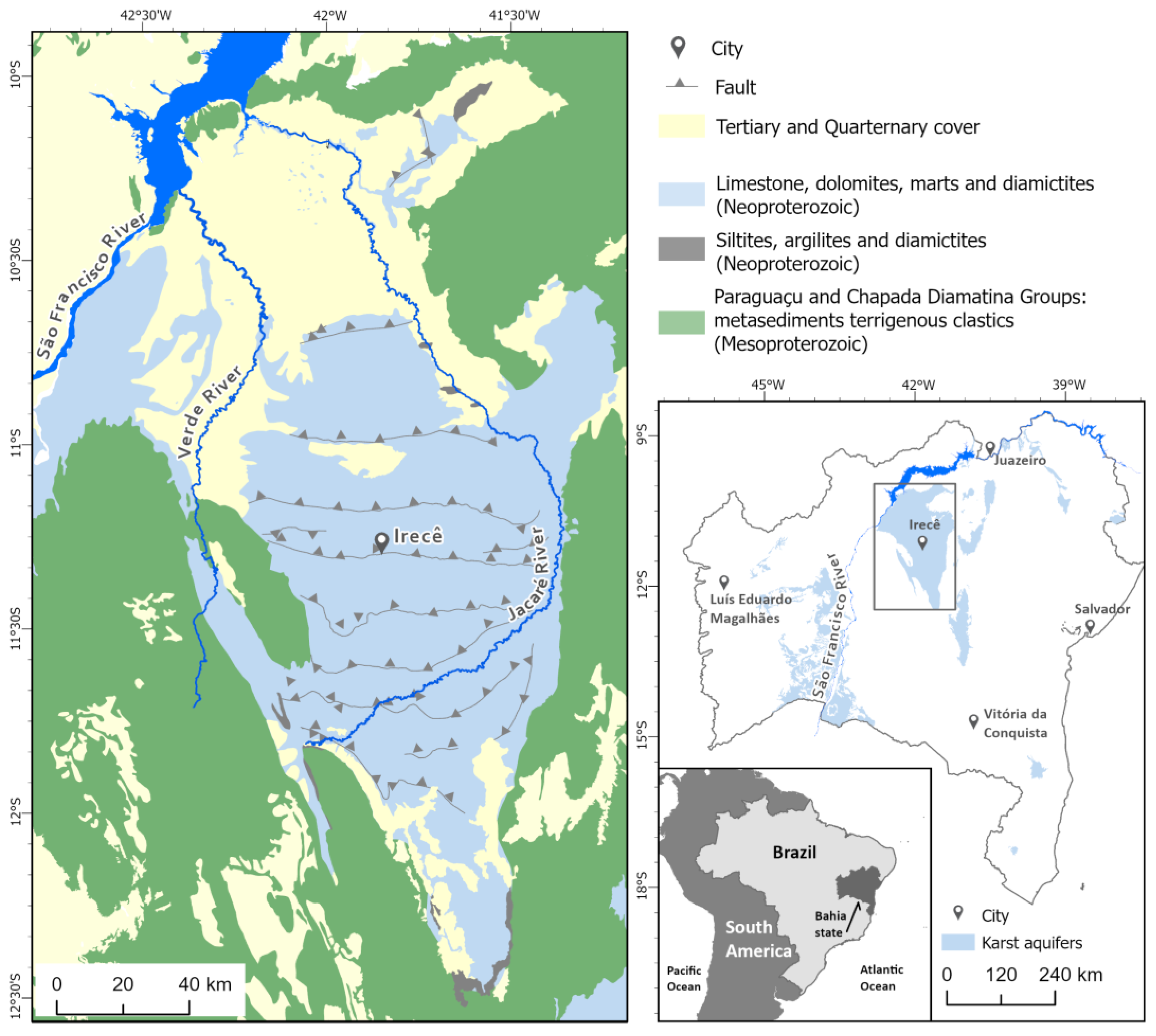
2.1. Study Area and Hydrogeological Conditions

The SKA is located in the central portion of the Chapada Diamantina, Bahia, Brazil (Figure 1). It is an unconfined aquifer with fissural and karstic porosity, formed by an extensive plateau of Precambrian (Neoproterozoic) carbonate rocks, with altitudes around 800 m above sea level and thicknesses that can reach up to 900 m [27,28,29]. The carbonate plateau is carved by the drainages of the Verde, Jacaré, and São Francisco rivers and is surrounded by a region of mountains composed of siliciclastic rocks from the Bebedouro Formation and the Paraguaçu and Chapada Diamantina Groups, also of Precambrian ages, with an average altitude of approximately 1500 m [28,30]. The sequence of carbonate rocks is partially covered by a thin layer of Tertiary and Quaternary detrital sediments.

The carbonate rocks that make up the SKA are represented by a sequence of limestone and dolomite layers that constitute the Salitre Formation, which is subdivided into the Nova América and Jussara lithostratigraphic units, respectively [31,32]. These rocks have been deformed and metamorphosed by successive tectono-metamorphic events that occurred during the Neoproterozoic era in association with the formation of mobile belts along the margins of the São Francisco Craton [28,33].

The deformation of the rocks is marked by the presence of folding systems, faults, fractures, and structural lineaments that guide the development of surface and subsurface karst features, forming a network of multiple conduits and channels for the storage and circulation of groundwater. This complexity makes it even more challenging to map zones with higher potential for drilling wells and groundwater extraction [26,31,32,33,34]. The main fracturing systems associated with most groundwater wells are represented by subvertical systems with N-S and NNE-SSW directions [27,35,36,37]. In contrast, the anticline folds influence the formation of caves and paleokarst tunnels exposed above the water table, which are frequently visited for speleological tourism [38,39].

The region is predominantly semi-arid with an average annual temperature of 23 °C (ranging between 15 °C and 34 °C). The average precipitation is 680 mm/year, concentrated mainly during the summer, while the annual evapotranspiration is approximately 1860 mm/year [40]. Regional groundwater flow diverges from areas of higher elevations towards the main river valleys (Figure S1). There are only two major rivers, with the Verde River being the only fully perennial one, while the Jacaré River has both perennial and intermittent stretches and periods [41] (Figure S6). Cambisols are the most common soils in the region [42]. The soils are highly fertile, and, combined with the availability of groundwater, the Irecê region has gained national prominence as a major producer of agricultural products such as onions, tomatoes, carrots, and castor beans. However, events of subsidence and sinkhole collapse have been recorded in rural and urban areas due to the overexploitation of groundwater in segments of the central and southern portions of the aquifer [43,44].

The annual recharge of the SKA, estimated from a hydrometeorological water balance, varies between 55 and 65 mm per year, which represents approximately 7% of the total precipitation. The periods of infiltration are more intense during the rainy season, from November to March [45]. Recharge is divided into autogenic and allogenic types; the former originates exclusively from precipitation directly on the karst outcrops [25,38], while the latter comes from groundwater flow through underlying rocks or surface waters emanating from the mountainous areas of the Chapada Diamantina Group surrounding the karst plateau [27].

Figure 1. Geological map [46] of the study area, showing the lithotypes of the Salitre Karst Aquifer (SKA), the Chapada Diamantina Group (CDG), and detrital cover. Non-English words are city and river names. For further maps, vertical cross-sections and river discharge time series, see Supporting Information.

Figure 1. Geological map [46] of the study area, showing the lithotypes of the Salitre Karst Aquifer (SKA), the Chapada Diamantina Group (CDG), and detrital cover. Non-English words are city and river names. For further maps, vertical cross-sections and river discharge time series, see Supporting Information.

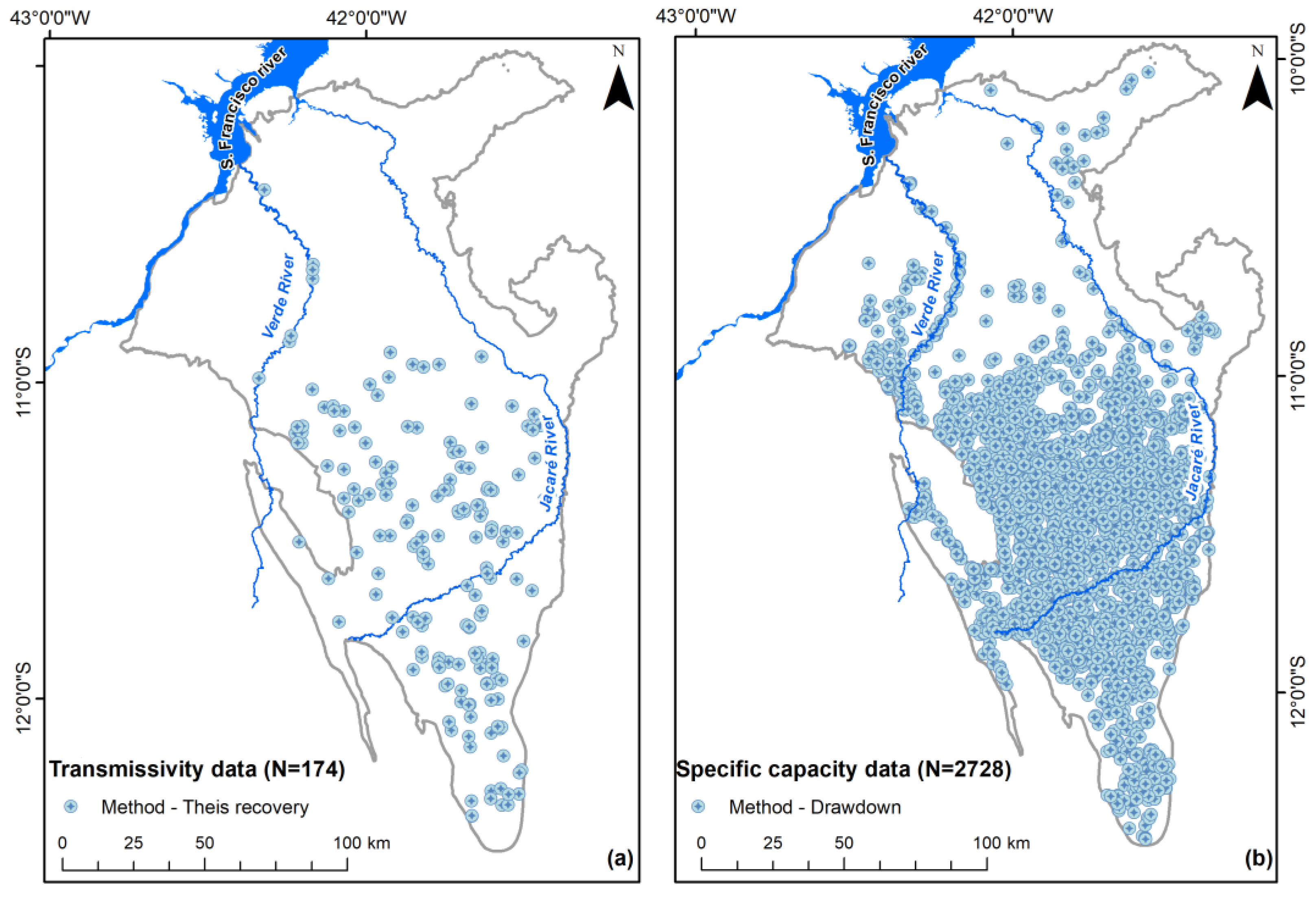
2.2. Data and Well Characteristics

The data from tubular wells used for this study were obtained from the well databases for groundwater extraction from the Bahia Water Engineering and Sanitation Company (CERB) and the Geological Survey of Brazil (SGB). These wells are used for both public and private supply, including residential use and irrigated agriculture. For the first set of data (Figure 2a), 174 data points from pumping and recovery tests were used to calculate the values of transmissivity (T) and specific capacity (S_c) using Theis’s recovery method (1935) [3]. The second group of data (Figure 2b) refers to specific capacity (S_c) values obtained from 2728 wells in pumping tests with insufficient data for estimating T.

Table 1. Statistical summary of hydraulic characteristics of wells in the SKA.

Parameters	Min 1	Max 2	Mean	Median	SD 3	CV 4
Pumping rate (m3/d)	2	8544	383	288	452	1
Water table depth (m)	0	147	26	20	21	1
Water entrance depths (m)	4.5	196	62	54	37	0.6
Well depth (m)	0	294	105	100	40	0.4

Note(s): ¹ minimum; ² maximum; ³ standard deviation; ⁴ coefficient of variation.

presents the average flow rates of the wells in the SKA, with values averaging 383 m³/day and reaching up to 8544 m³/day. The average depth of water levels below ground is 26 m, with depths reaching up to 147 m. Since this is an aquifer with dual porosity due to interconnected fracture systems and karst conduits, water entries (i.e., intersections of wells with fractures or water-bearing conduits) occur at depths greater than 4.5 m and sometimes close to 200 m. It can be seen in Table 1 that the maximum depth of the wells can reach approximately 300 m, representing possibly unsuccessful attempts to reach water-bearing conduits at greater depths.

2.3. Linear Correlation

Values of T and S were calculated using Theis’s recovery method and the drawdown method for single wells, respectively. The correlation between these two parameters was established through a linear regression model after applying decimal logarithmic transformations (denoted as logT and logS_c) to obtain approximately normal distributions of the data. The quality of the linear model was evaluated using the Shapiro–Wilk normality test [47].

2.4. Cross-Variogram

The cross-semi-variogram ${\gamma }_{x,y}$(short “cross-variogram” hereafter) is a function that describes the degree of spatial continuity between two or more variables ($Z_x \mathrm{and} Z_y$, here represented by logT and logS_c) that are linearly correlated between coordinates $x_i \mathrm{and} x_i+h$, where $N\left(h\right)$ represents the number of available data pairs as a function of separation distance $\left(h\right)$, as presented in Equation (1).

$${\mathit{\gamma }}_{\mathit{x},\mathit{y}}\mathbf{\left(}\mathit{h}\mathbf{\right)}\mathbf{=}{\displaystyle \frac{\mathbf{1}}{\mathbf{2}\mathit{N}\mathbf{\left(}\mathit{h}\mathbf{\right)}}}{{\displaystyle \mathbf{\sum }}}_{\mathit{i}\mathbf{=}\mathbf{1}}^{\mathit{N}\mathbf{\left(}\mathit{h}\mathbf{\right)}}\mathbf{[}\mathbf{(}{\mathit{Z}}_{\mathit{x}}\mathbf{\left(}{\mathit{x}}_{\mathit{i}}\mathbf{\right)}\mathbf{-}{\mathit{Z}}_{\mathit{x}}\mathbf{\left(}{\mathit{x}}_{\mathit{i}}\mathbf{+}\mathit{h}\mathbf{\right)}]\mathbf{\left[}{\mathit{Z}}_{\mathit{y}}\mathbf{\left(}{\mathit{x}}_{\mathit{i}}\mathbf{\right)}\mathbf{-}{\mathit{Z}}_{\mathit{y}}\mathbf{\left(}{\mathit{x}}_{\mathit{i}}\mathbf{+}\mathit{h}\mathbf{\right)}\mathbf{\right]}$$

(1)

Unlike the classic (univariate) variogram, the cross-variogram allows for negative values, since the relationships between variables can occur in an inverse proportion. Cross-variograms can be defined as colocated and non-colocated. In this work, we used the colocated CO-OK model [48], since the data from T and S_c had the same coordinate at 174 points.

2.5. Linear Model of Coregionalization

The Linear Model of Coregionalization (LMC) represents a linear combination of basic components, where the variogram functions of each component must be non-negative. The Cauchy–Schwarz inequality, represented by $\left({\gamma }_{x,y}\right)²\le ({\gamma }_x\times {\gamma }_y$)), where ${\gamma }_{x,y}$ represents the sill of the crossed variogram, while ${\gamma }_x$ and ${\gamma }_y$ are the sill of the primary and secondary variables, modeled separately, can also be used as a verification criterion for the LMC [16].

2.6. Ordinary Co-Kriging

Ordinary co-kriging (CO-OK) is a multivariate extension of ordinary kriging, where one or more auxiliary variables are used to estimate the values of the primary variable at unsampled locations. Its implementation depends on the construction of a valid LMC cross-variogram. Ordinary co-kriging produces smaller estimation errors compared to ordinary (univariate) kriging. The values estimated by CO-OK at coordinate ${\mathit{x}}_{\mathbf{0}}$ is ${\mathit{Z}}^{\mathbf{*}}$, as shown in Equation (2). The sets ${\mathit{S}}_{\mathbf{1}} \mathbf{and} {\mathit{S}}_{\mathbf{2}}$ and the values ${\mathit{Z}}_{\mathbf{1}} \mathbf{and} {\mathit{Z}}_{\mathbf{2}}$ represent the primary and secondary variables, respectively [48]. The weights of the linear combination of the primary and secondary variables are represented by ${\mathit{\lambda }}_{\mathbf{1}\mathit{\alpha }} \mathbf{and} {\mathit{\lambda }}_{\mathbf{2}\mathit{\alpha }}$ [16]. We used the number of neighbors “m”. The ordinary co-kriging presented in this study was performed on a grid containing 88,268 cells with dimensions of 500 by 500 m, using 174 values of logT and 2728 values of logS_c.

$${\mathit{Z}}^{\mathbf{*}}\mathbf{\left(}{\mathit{x}}_{\mathbf{0}}\mathbf{\right)}\mathbf{=}{{\displaystyle \mathbf{\sum }}}_{{\mathit{S}}_{\mathbf{1}}}{\mathit{\lambda }}_{\mathbf{1}\mathit{\alpha }}{\mathit{Z}}_{\mathbf{1}}\mathbf{\left(}{\mathit{x}}_{\mathit{\alpha }}\mathbf{\right)}\mathbf{+}{{\displaystyle \mathbf{\sum }}}_{{\mathit{S}}_{\mathbf{2}}}{\mathit{\lambda }}_{\mathbf{2}\mathit{\alpha }}{\mathit{Z}}_{\mathbf{2}}\mathbf{\left(}{\mathit{x}}_{\mathit{\alpha }}\mathbf{\right)}$$

(2)

2.7. Conditional Gaussian Co-Simulation

Conditional sequential Gaussian co-simulation (CO-SGS) is a multivariate counterpart of sequential Gaussian simulation. These methods are widely used to generate estimated representations of an area based on a set of samples, considering both the distribution law of the variable under study and its spatial continuity. We performed a total of 60 simulations to obtain an adequate number of realizations, varying from 10 to 600 per simulation. In each simulation, we calculated the variance at each grid point based on the corresponding number of realizations and determined the spatial average of these variances. We observed that the mean variance increased with the number of realizations but tended to stabilize when the number was sufficient to adequately represent the entire variability of the process. To evaluate the adequacy of the number of simulations, we calculated the mean variance increment (MVI) from one simulation to the next, using the proximity of this increment to zero as a criterion. Based on the distribution of simulated transmissivity values at each grid location, we calculated the expectations, standard deviations, and probabilities of not exceeding certain value thresholds.

3. Results

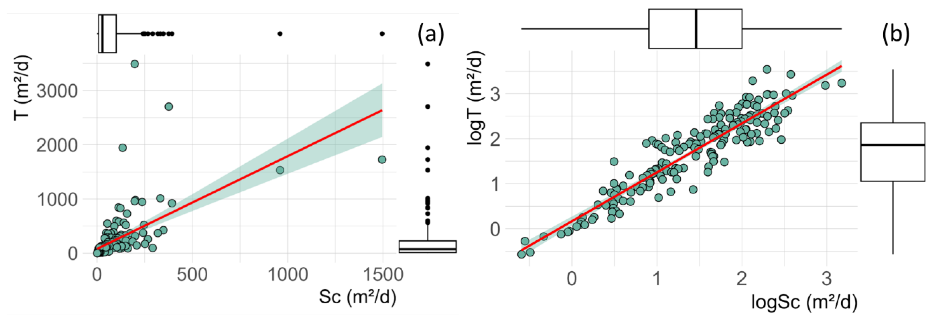
3.1. Linear Correlation between logS_c and logT

Table 2. Statistical summary of T and S_c (both in m²/d) and their respective logarithms for N = 174 wells (Figure 2a).

Attributes	Min 1	Max 2	Mean	Median	SD 3	CV 4
Sc	0.25	1495	77.7	29	152.7	1.94
logSc	−0.59	3.17	1.89	1.46	2.18	0.29
T	0.27	3.49	211.48	73.45	433.96	2.05
logT	−0.56	3.54	2.3	1.87	0.89	0.38

Note(s): ¹ minimum; ² maximum; ³ standard deviation; ⁴ coefficient of variation.

presents the values of 174 collocated pairs of T and S_c, along with their decimal logarithms. We observed that the average values of S_c and T were 77.7 m²/d and 211.48 m²/d, respectively, with both displaying high standard deviations, justifying the use of the logarithmic transformation for better data manipulation. The distribution of the logT and logS_c values was more symmetrical compared to that of T and S_c, as evidenced by the significant reduction in the coefficients of variation. The skewness of the parameters reflects the heterogeneity attributed to the local karst system, as observed in other studies [9,11,49].

The boxplots presented in Figure 3a predominantly show low values for both parameters, making it difficult to identify a fitted line. In contrast, Figure 3b demonstrates the greater symmetry of the boxplots, allowing for a linear adjustment after the logarithmic transformation. The Shapiro–Wilk normality test (1965) for both logT and logS_c resulted in p-values of approximately 0.01. This indicates that the null hypothesis of normality was rejected for both variables.

LogT and logS_c showed a strong linear correlation (Figure 3b), as indicated by the coefficient of determination R² = 0.86 (p < 2.2 × 10⁻¹⁶). The strong correlation shown in Figure 3b can be used to estimate values of empirical transmissivities T_emp, as shown in Equation (3). Strong correlations between the described variables, as well as empirical models, have also been observed in other karst aquifers [12,50,51].

$${\mathit{T}}_{\mathit{e}\mathit{m}\mathit{p}} \mathbf{=} \mathbf{0.17}{\mathit{S}}_{\mathit{c}}^{\mathbf{1.09}}$$

(3)

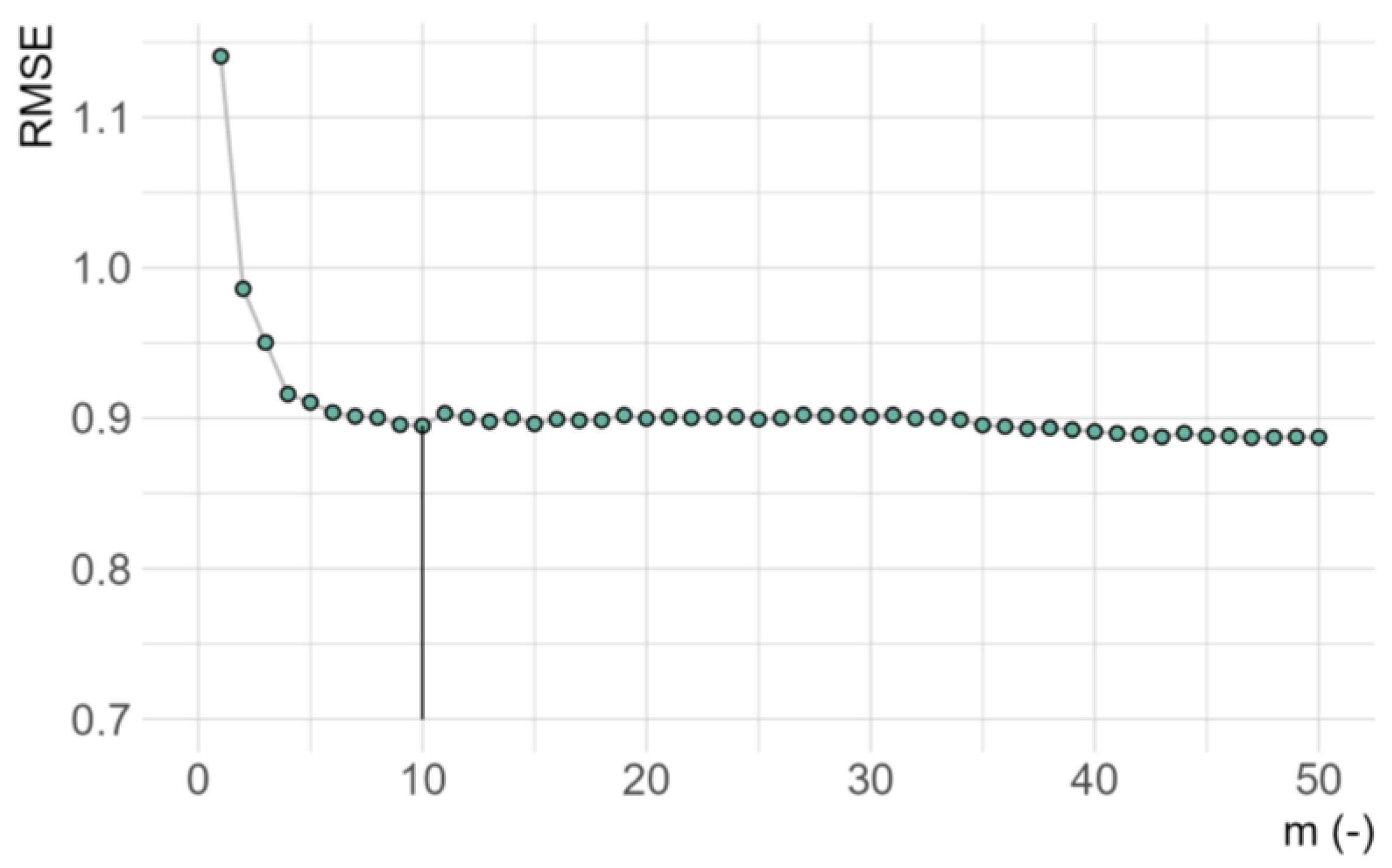
3.2. Spatial Structure and Linear Model of Coregionalization

The spatial continuity of the logT and logS_c values was analyzed by modeling the univariate and cross-variograms (logT × logS_c) of both parameters. In the variogram presented in Figure 4, we considered the samples of the 174 logT and logS_c values under the same coordinates using the following azimuth directions: 0, 22.5, 45, 67.5, 90, 112.5, 135, and 157.5, resulting in an omnidirectional model as the most suitable. The cross-variogram showed an exponential structure, a sill of 0.65, a nugget effect of 21% of the sill, and a range of 5 km. The cross-variogram in Figure 4 respected the Cauchy–Schwartz inequality postulate ((0.62)² ≤ (0.78 × 0.57) and (0.13)² ≤ (0.16 × 0.13)) for the sill and nugget effect, respectively, thus indicating a valid LMC.

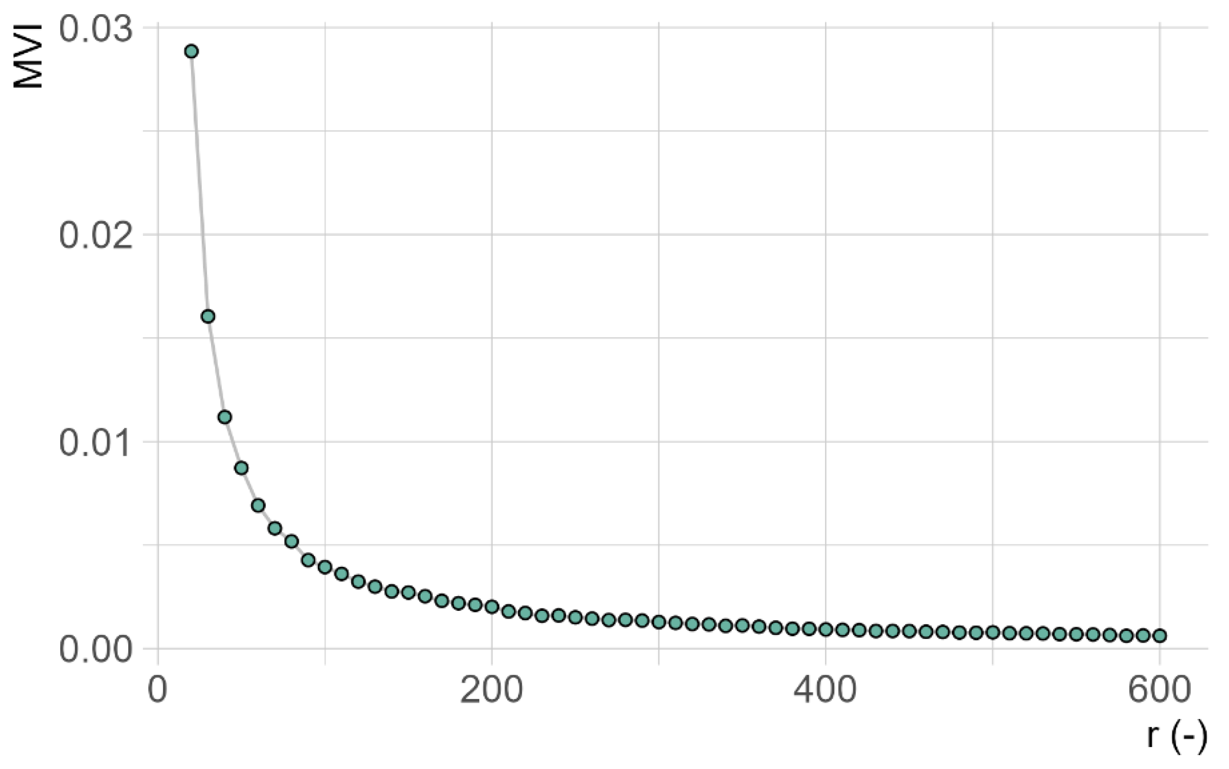
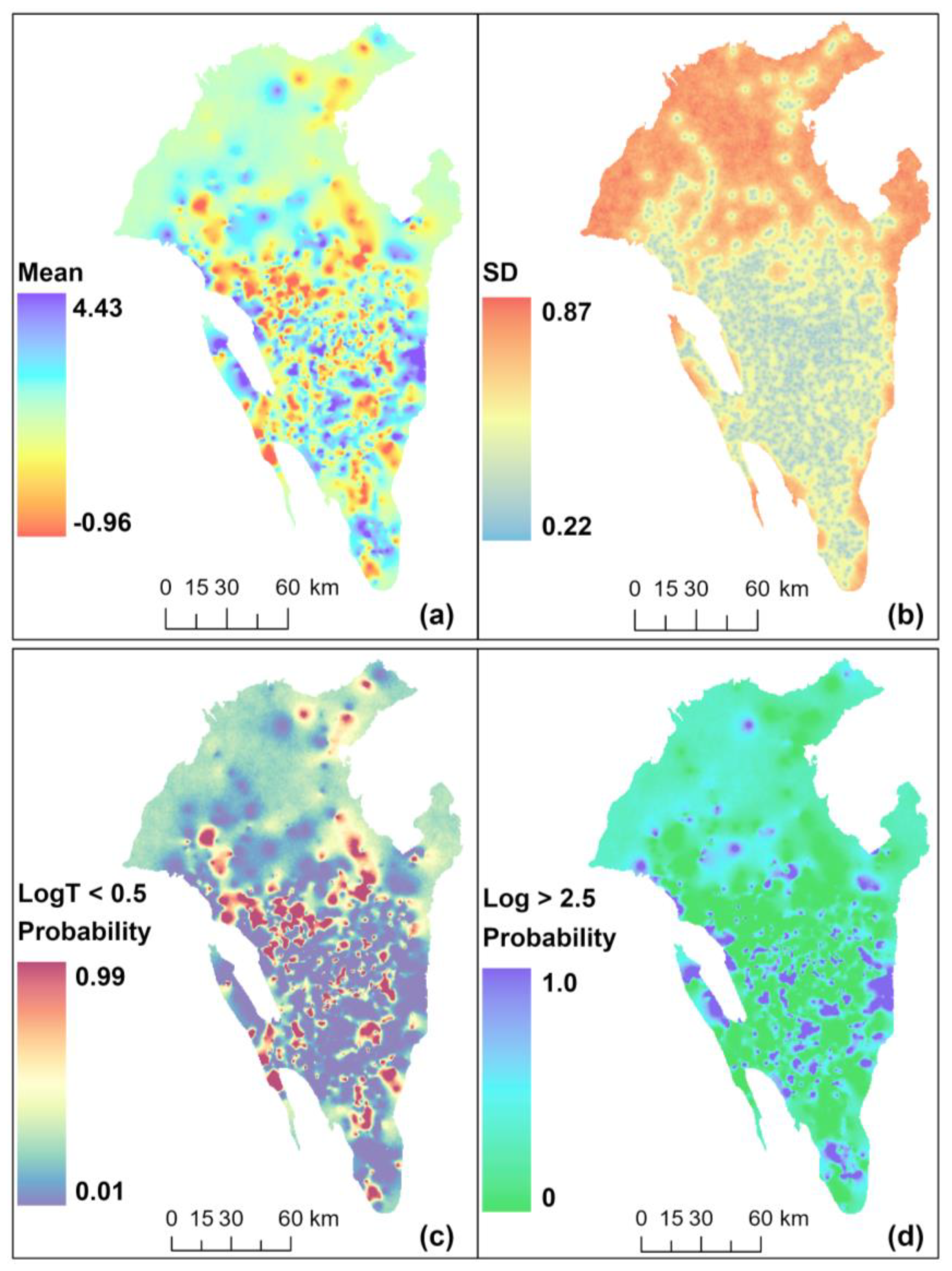
3.3. Interpolation and Uncertainty

Ordinary co-kriging (CO-OK) was performed, as presented in Equation (2), where we used the cross-variogram shown in Figure 4 and the optimal number of neighboring wells (m). The estimation of m was carried out through the cross-validation presented in Figure 5, where we obtained m = 10 and an RMSE of 0.9 for the logT values. However, the nugget effect of the cross-variogram showed an intermediate degree of randomness.

In the map shown in Figure 6a, the interpolation resulting from CO-OK is spatially represented, while Figure 6b shows the associated standard deviations. We observed that the highest logT values are near the edges of the SKA and in the southern portion, where they exceed the magnitude of logT = 3 m²/d (greater than 1000 m²/d). In the edge domains of the aquifer, we can associate the high logT values with the contact between the carbonate lithotypes of the SKA and the siliciclastic rocks of the CDG, enhanced by the brittle structures that increase storage in these locations. In the southern portion, a more evolved karst is observed compared to other sectors of the SKA, where, in addition to the brittle structures, there are deep caves with high storage capacity associated with hypogenic karstification [24]. The most karstified zones observed in the southern portion of the aquifer are characterized by negative gravimetric anomalies at depths of up to 50 m, while at greater depths, cavities capable of storing large volumes of water are also observed [52]. The other zones with high logT values are distributed randomly, with logT > 2 m²/d (>100 m²/d). In the northern domain of the SKA, areas with higher uncertainties predominate, which are associated with a low density of tubular wells.

3.4. Co-Simulation and Probability Maps

The stochastic simulation conducted in this study generated MVI values close to zero for a total of 500 realizations (Figure 7), establishing this as the appropriate number for conditional realizations in the adopted stochastic co-simulation. In Figure 8a, the mean values of the combined realizations of logT and logS_c are presented, while the standard deviation map is shown in Figure 8b. The results of the mean CO-SGS (500 realizations) were similar to those of the logT co-kriging (Figure 6a), reflecting the consistency of the mathematical principles underlying both methods. A similar spatial distribution of deviations was also observed, with high uncertainties in areas with low data density. The range of simulated standard deviations was 80% greater than the values obtained by co-kriging, revealing a greater variation compared to the kriged logT values, especially in the southern region of the SKA [12].

Figure 8c shows a map of the probabilities of occurrence of logT < 0.5 m²/d (approximately 3 m²/d), representing the zones with the lowest groundwater potential of the SKA in dark red color. In contrast, the map in Figure 8d illustrates the probabilities of occurrences for logT values greater than 2.5 m²/d, highlighting the areas with the highest groundwater availability in deep blue.

4. Discussion

4.1. Regression and Co-Kriging

In this study, we obtained an empirical linear regression model based on 174 paired values of logT and logS_c as ${\mathit{T}}_{\mathit{e}\mathit{m}\mathit{p}} \mathbf{=} \mathbf{0.17}{\mathit{S}}_{\mathit{c}}^{\mathbf{1.09}}$. For comparison with Gonçalves et al. (2024) [12], we spatialized logT_emp from 2728 logS_c values and obtained an omnidirectional variogram with an exponential structure, a sill of 1.17, a nugget effect of approximately 50% of the sill, and a range of 3 km (Figure S2). The crossed variogram presented in this work (Figure 4) proved to be less random compared to that in Figure S2.

We used the same values of m (Figure 5) and r (Figure 7) to generate maps of ordinary kriging—OK —(Figure S3a) and standard deviations associated with interpolation (Figure S3b). The uncertainties resulting from CO-OK also presented lower values compared to the ordinary kriging presented in Figure S3a, highlighting the positive effects on error reduction of CO-OK compared to ordinary kriging (OK).

In Figure S4a, we present the results of the averages of 500 stochastic realizations for logT_emp, and in Figure S4b, the standard deviations are presented. We verified that the average logT_emp values (Figure S4a) generated by SGS varied in the same order of magnitude compared to the average logT values (Figure S4b) generated by CO-SGS, but the standard deviations (SD) generated by SGS (0.75–1.24) were higher when we applied CO-SGS (0.22–0.87).

Previous works [35,36,52] highlight significant structural control in the rocks of the SKA, where the development of voids in the rocks is controlled by faults and fracture systems. However, this characteristic did not materialize in the structural anisotropy of the variogram, indicating the presence of a system of secondary conduits connected to the main conduits (controlled by structure), resulting in an interconnected network of underground channels [52]. These interconnections between conduits can be observed in other Precambrian karst systems, such as the Sete Lagoas Formation, where groundwater storage in conduit and fracture systems has been verified [53].

Groundwater potential in karst aquifers can be assessed by the transmissivity of the aquifer. Previous studies have shown that geomorphological elements are diagnostic factors of greater or lesser favorability for groundwater storage and transmissivity [8,54]. We correlated transmissivity with other geomorphological elements, including wellhead elevation, slope, structural photolineament density, sinkhole density, distance to brittle structures, and distance to the main rivers of the SKA, as shown in Figure S5. However, we did not observe moderate or strong correlations between the logT values and these geomorphological attributes, with the maximum linear correlation coefficient obtained being 0.1 (absolute value), resulting from the linear correlation between logT and elevation.

Although we did not observe a strong correlation between transmissivity and geomorphological factors in the SKA, we did find that the sections with the highest flow of the Verde and Jacaré rivers were located in areas with logT > 2.5 m²/d (Figure S6). Thus, groundwater in high-transmissivity zones significantly contributes to maintaining the perennial flow of the Verde and Jacaré rivers. Excessive groundwater exploitation in these areas may lead to a significant reduction in the base flow of these rivers.

4.2. Cross-Variogram and Multivariate Interpolation

The cross-variogram in Figure 4 shows a low nugget effect (21% of the sill), indicating less randomness compared to previous studies. Cross-variograms of logT with logS_c were modeled in fissured, highly heterogeneous aquifers, where the nugget effect represented approximately 51% of the sill [7]. In a similarly heterogeneous but granular aquifer, the proportion of the nugget effect in the cross-variogram sill was 25% [55]. When analyzing individual variograms (logT_emp) only in the southern portion of the SKA, a nugget effect above 50% was observed [12]. Therefore, the domains with greater heterogeneity in the SKA are associated with the most karstified areas (mainly in the southern portion), while lower heterogeneity is linked to regions where the SKA is predominantly fissured.

In the ordinary kriging shown in Figure S3a, a slightly smaller range of logT_emp values was observed (varying between −0.88 m²/d and 3.03 m²/d) compared to the co-kriged logT values (varying between 0.2 m²/d and 3.9 m²/d). The standard deviations shown in Figure S2 also showed a smaller range compared to those obtained in the co-kriging shown in Figure 6. The reduction between the maximum standard deviation values for logT_emp and logT derived from ordinary kriging and ordinary co-kriging, respectively, was 0.19, while the reduction in terms of the minimum standard deviations was 0.65. This reduction in estimation uncertainty illustrates the benefit of using S_s as a secondary variable in a multivariate ordinary co-kriging approach.

In a comparison between CO-SGS and SGS presented by Gonçalves et al. (2024) [12], considering only the southern portion of the SKA, significant differences between the two models can be observed. Firstly, the logT_emp values generated by SGS vary within a smaller range, between 1 m²/d and 2.8 m²/d, while the logT values estimated by CO-SGS vary between −0.2 m²/d and 3.4 m²/d. The standard deviations also differ, varying between 0.6 and 0.9 for SGS and between 0.25 and 0.82 for CO-SGS. In other words, the reductions in the standard deviations were similar compared to the uncertainties generated by OK. These results clearly show improved confidence due to the adoption of CO-OK and CO-SGS estimates in the interpolation of logT values in the SKA.

5. Conclusions

In this study, we used ordinary co-kriging and conditional sequential Gaussian co-simulation to spatially interpolate the hydraulic transmissivity T based on 174 measured values of T and 2728 measured values of the specific capacity S_c. We verified the strong linear and structural correspondences between 174 pairs of logT and logS_c values sampled at the same locations. The observed correlations enabled the construction of a cross-variogram, with a valid LMC, which showed an isotropic structure, low nugget effect, range of 5 km, and sill equal to 0.62.

Cross-validation indicated an optimal number of 10 neighbors (RMSE = 0.9), and 500 was the number of stochastic realizations used. Both methodologies (CO-OK and CO-SGS) showed equivalent values for the means of the logT estimates, with a stochastic pattern in the distribution of the logT values in the SKA. In regions with a low well density, both models showed the highest uncertainties, especially in the northern sector of the SKA, where the greatest uncertainties are concentrated due to a very limited number of wells. The multivariate geostatistical methods (CO-OK and CO-SGS) used in this work generated smaller uncertainties when compared to univariate methods (OK and SGS).

The delimitation of areas with greater uncertainties presented in this study also enables future actions to increase the sampling density and integrate geophysical data, since more accurate transmissivity estimates are fundamental for the design of groundwater management strategies, including the location of tubular wells, artificial recharge projects, and numerical flow modeling.

The results obtained demonstrate a significant advance compared to previous studies, increasing knowledge about the heterogeneities and uncertainties of the SKA. This advance in transmissivity mapping also brings important contributions to the field of applied geostatistics, showing how this tool can be applied in the mapping of hydrodynamic parameters in Precambrian karst aquifers present in semi-arid climates, a rare example in the scientific literature. Furthermore, the results obtained should guide the sustainable management of water resources, providing support for well drilling, artificial recharge projects, and numerical flow modeling.

References

1. Stevanović, Z. Karst Waters in Potable Water Supply: A Global Scale Overview. Environ. Earth Sci. 2019, 78, 662. [Google Scholar] [CrossRef]
2. Ford, D.; Williams, P. Karst Hydrogeology and Geomorphology, 1st ed.; Wiley: Hoboken, NJ, USA, 2007; ISBN 9780470849965. [Google Scholar]
3. Theis, C.V. The Relation between the Lowering of the Piezometric Surface and the Rate and Duration of Discharge of a Well Using Ground-water Storage. Eos Trans. AGU 1935, 16, 519–524. [Google Scholar] [CrossRef]
4. Bouwer, H.; Rice, R.C. A Slug Test for Determining Hydraulic Conductivity of Unconfined Aquifers with Completely or Partially Penetrating Wells. Water Resour. Res. 1976, 12, 423–428. [Google Scholar] [CrossRef]
5. Barker, J.A. A Generalized Radial Flow Model for Hydraulic Tests in Fractured Rock. Water Resour. Res. 1988, 24, 1796–1804. [Google Scholar] [CrossRef]
6. Mace, R.E. Determination of Transmissivity from Specific Capacity Tests in a Karst Aquifer. Groundwater 1997, 35, 738–742. [Google Scholar] [CrossRef]
7. Razack, M.; Lasm, T. Geostatistical Estimation of the Transmissivity in a Highly Fractured Metamorphic and Crystalline Aquifer (Man-Danane Region, Western Ivory Coast). J. Hydrol. 2006, 325, 164–178. [Google Scholar] [CrossRef]
8. Srivastav, S.K.; Lubczynski, M.W.; Biyani, A.K. Upscaling of Transmissivity, Derived from Specific Capacity: A Hydrogeomorphological Approach Applied to the Doon Valley Aquifer System in India. Hydrogeol. J. 2007, 15, 1251–1264. [Google Scholar] [CrossRef]
9. Galvão, P.; Halihan, T.; Hirata, R. Transmissivity of Aquifer by Capture Zone Method: An Application in the Sete Lagoas Karst Aquifer, MG, Brazil. An. Acad. Bras. Ciênc. 2017, 89, 91–102. [Google Scholar] [CrossRef]
10. Gonçalves, T.S. Quantitative Models for Estimating Transmissivity in the Salitre Aquifer in the Region of Irecê–Ba, Brazil. Master’s Thesis, Institute of Geosciences, Federal University of Bahia, Salvador, Brazil, 2017. (In Portuguese with English Abstract). [Google Scholar]
11. Gonçalves, T.S.; Leal, L.R.B. Potencialidades Hídricas No Aquífero Carstico Salitre Na Região de Irecê, Bahia. R. Águas Subter. 2018, 32, 191–199, (In Portuguese with English Abstract). [Google Scholar] [CrossRef]
12. Gonçalves, T.S.; Klammler, H.; Bastos Leal, L.R. Geospatial Analysis of Transmissivity and Uncertainty in a Semi-Arid Karst Region. Water 2024, 16, 780. [Google Scholar] [CrossRef]
13. Kitanidis, P.K. Introduction to Geostatistics: Applications to Hydrogeology; Cambridge University Press: Cambridge, UK; New York, NY, USA, 1997; ISBN 9780521583121. [Google Scholar]
14. Aboufirassi, M.; Mariño, M.A. Cokriging of Aquifer Transmissivities from Field Measurements of Transmissivity and Specific Capacity. Math. Geol. 1984, 16, 19–35. [Google Scholar] [CrossRef]
15. Ahmed, S.; De Marsily, G. Comparison of Geostatistical Methods for Estimating Transmissivity Using Data on Transmissivity and Specific Capacity. Water Resour. Res. 1987, 23, 1717–1737. [Google Scholar] [CrossRef]
16. Wackernagel, H. Multivariate Geostatistics; Springer: Berlin/Heidelberg, Germany, 2003; ISBN 9783642079115. [Google Scholar]
17. Gloaguen, E.; Chouteau, M.; Marcotte, D.; Chapuis, R. Estimation of hydraulic conductivity of an unconfined aquifer using cokriging of GPR and hydrostratigraphic data. J. Appl. Geophys. 2001, 47, 135–152. [Google Scholar] [CrossRef]
18. Zangeneh, D.K.; Amanipoor, H.; Battaleb-Looie, S. Evaluation of heavy metal contamination using cokriging geostatistical methods (case study os Abteymour oilfield in southern Iran). Appl. Water Sci. 2023, 13, 200. [Google Scholar] [CrossRef]
19. Journel, A.G.; Rossi, M.E. When Do We a Trend Model in kriging? Math. Geol. 1989, 21, 715–739. [Google Scholar] [CrossRef]
20. Larocque, G.; Dutilleul, P.; Pelletier, B.; Fyles, J.W. Conditional Gaussian Co-Simulation of Regionalized Components of Soil Variation. Geoderma 2006, 134, 1–16. [Google Scholar] [CrossRef]
21. Schiavo, M. Numerical impact of variable volumes of Monte Carlo simulations of heterogeneous conductivity fields in groundwater flow models. J. Hydrol. 2024, 634, 131072. [Google Scholar] [CrossRef]
22. Aliouache, M.; Jourde, H. Influence of structural properties and connectivity of initial fracture network on incipient karst genesis. J. Hydrol. 2024, 640, 131684. [Google Scholar] [CrossRef]
23. 2022 Demographic Census of Brazil-IBGE. Available online: https://www.ibge.gov.br/censo2022 (accessed on 26 July 2024).
24. Salles, L.Q.; Bastos Leal, L.R.; Pereira, R.G.F.D.A.; Laureano, F.V.; Gonçalves, T.S. Influence of the Hydrogeological Aspects of Karst Aquifers on Landscape Evolution: Central Portion of the Diamantina Plateau, Bahia, Brazil. Rev. Bras. Geomorfol. 2018, 19, 93–106, (In Portuguese with English Abstract). [Google Scholar] [CrossRef]
25. Silva, H.M. Geographic Information System of the Karst Aquifer of the Microregion of Irecê, Bahia: Subsidy for the Inte-Grated Management of the Water Resources of the Verde and Jacaré River Basins. Master’s Thesis, Federal University of Bahia, Salvador, Brazil, 2005. [Google Scholar]
26. Guerra, A.M. Karstification Processes and Hydrogeology of Bambuí Group at Irecê Region, Bahia. Doctoral Thesis, University of São Paulo, São Paulo, Brazil, 1986. (In Portuguese with English Abstract). [Google Scholar]
27. Bastos Leal, L.R.; Dutton, A.R.; Luz, J.G.; Barbosa, J.S.F. Hydrogeology and hydrochemistry of a Precambrian karst aquifer in a semi-arid region from Bahia, Brazil. In Proceedings of the Geological Society of America, Annual Meeting 2006, Philadelphia, PA, USA, 22–25 October 2006; p. 286. [Google Scholar]
28. Misi, A.; Kaufman, A.J.; Azmy, K.; Dardenne, M.A.; Sial, A.N.; De Oliveira, T.F. Chapter 48 Neoproterozoic Successions of the São Francisco Craton, Brazil: The Bambuí, Una, Vazante and Vaza Barris/Miaba Groups and Their Glaciogenic Deposits. Memoirs 2011, 36, 509–522. [Google Scholar] [CrossRef]
29. Feitosa, F.A.C.; Diniz, J.A.O.; Kirchheim, R.E.; Kiang, C.H.; Feitosa, E.C. Assessment of Groundwater Resources in Brazil: Current Status of Knowledge. In Groundwater Assessment, Modeling, and Management; CRC Press: Boca Raton, FL, USA, 2016; Available online: https://www.routledgehandbooks.com/doi/10.1201/9781315369044-5 (accessed on 5 August 2023).
30. Laipelt, L.; Comini de Andrade, B.; Collischonn, W.; de Amorim Teixeira, A.; Paiva, R.C.D.d.; Ruhoff, A. ANADEM: A Digital Terrain Model for South America. Remote Sens. 2024, 16, 232. [Google Scholar] [CrossRef]
31. Pedreira, A.J. The Espinhaço Supergroup in the Central-Eastern Chapada Dia mantina, Bahia: Sedimentology, Stratigraphy and Tectonics. Doctoral Thesis, University of São Paulo, São Paulo, Brazil, 2004. (In Portuguese with English Abstract). [Google Scholar]
32. Souza, S.L.; Brito, P.C.R.; Silva, R.W.S.; Pedreira, A.J. Stratigraphy, Sedimentology and Mineral Resources of the Salitre Formation in the Irecê Basin, Bahia; Arquivos Abertos; CBPM: Salvador, Brazil, 1993; Volume 2. (In Portuguese) [Google Scholar]
33. Misi, A.; Veizer, J. Neoproterozoic Carbonate Sequences of the Una Group, Irecê Basin, Brazil: Chemostratigraphy, Age and Correlations. Precambrian Res. 1998, 89, 87–100. [Google Scholar] [CrossRef]
34. Bastos Leal, L.R.; Silva, H.P. Hydrologic Model and Management of the Aquifer-River Sistem on the Verde and Jacaré Rivers–Semi-Arid Region of the Bahia State, Brazil; SRH/UFBA: Salvador, Brazil, 2004. (In Portuguese) [Google Scholar]
35. Furtado, C.P.Q.; Borges, S.V.F.; Bezerra, F.H.R.; De Castro, D.L.; Maia, R.P.; Teixeira, W.L.E.; Souza, A.M.; Auler, A.S.; Lima-Filho, F.P. The Fracture-Controlled Carbonate Brejões Karst System Mapped with UAV, LiDAR, and Electroresistivity in the Irecê Basin-Brazil. J. S. Am. Earth Sci. 2022, 119, 103986. [Google Scholar] [CrossRef]
36. Kuchenbecker, M.; Reis, H.L.S.; Fragoso, D.G.C. Structural Characterization and Considerations on the Tectonic Evolution of the Salitre Formation in the Central Portion of the Irecê Basin, North of the São Francisco Craton (BA). Geonomos 2011, 19, 42–49. (In Portuguese) [Google Scholar] [CrossRef]
37. Furtado, C.P.Q.; Medeiros, W.E.; Borges, S.V.; Lopes, J.A.G.; Bezerra, F.H.R.; Lima-Filho, F.P.; Maia, R.P.; Bertotti, G.; Auler, A.S.; Teixeira, W.L.E. The influence of subseismic-scale fracture interconnectivity on fluid flow in fracture corridors of the Brejões carbonate karst system, Brazil. Mar. Pet. Geol. 2022, 141, 105689. [Google Scholar] [CrossRef]
38. Auler, A.S.; Smart, P.L. The Influence of Bedrock-derived Acidity in the Development of Surface and Underground Karst: Evidence from the Precambrian Carbonates of Semi-arid Northeastern Brazil. Earth Surf. Process. Landf. 2003, 28, 157–168. [Google Scholar] [CrossRef]
39. Ennes-Silva, R.A.; Bezerra, F.H.R.; Nogueira, F.C.C.; Balsamo, F.; Klimchouk, A.; Cazarin, C.L.; Auler, A.S. Superposed Folding and Associated Fracturing Influence Hypogene Karst Development in Neoproterozoic Carbonates, São Francisco Craton, Brazil. Tectonophysics 2016, 666, 244–259. [Google Scholar] [CrossRef]
40. Meteorological Database of INMET. Available online: https://bdmep.inmet.gov.br/# (accessed on 17 July 2024).
41. Chagas, V.B.P.; Chaffer, P.L.B.; Addor, N.; Fan, F.M.; Fleischmann, A.S.; Paiva, R.C.D.; Siqueira, V.A. CAMELS-BR: Hydrometeorological time series and landscap attributes for 897 catchments in Brasil. Earth Syst. Data. 2020, 12, 2075–2096. [Google Scholar] [CrossRef]
42. de Paiva, A.Q. Carbonate-Phosphate Soils of the Irecê Plateau, BA: Genesis, Mineralogy and Geochemistry. Doctoral Thesis, Federal University of Viçosa, Viçosa, Brazil, 2010. (In Portuguese with English Abstract). [Google Scholar]
43. Salles, L.Q.; Galvão, P.; Bastos Leal, L.R.; De Araujo Pereira, R.G.F.; Purificação, C.G.C.; Laureano, F.V. Evaluation of Susceptibility for Terrain Collapse and Subsidence in Karst Areas, Municipality of Iraquara, Chapada Diamantina (BA), Brazil. Environ. Earth Sci. 2018, 77, 593. [Google Scholar] [CrossRef]
44. Maia, P.H.P.; Neto, B.D.; Corrêa-Gomes, L.C. Geological and Structural Analysis of Fissures and Subsidence in Lapão Karst. Águas Subterrâneas 2010, 7, 112–121. (In Portuguese) [Google Scholar]
45. Ramos, S.O.; Araújo, H.A.D.; Leal, L.R.B.; Luz, J.A.G.D.; Dutton, A.R. Temporal Variation of the Water Table in the Karst Aquifer of Irecê-Bahia: Contribution to the Use and Management of Groundwater in the Semi-Arid Region. RBG 2007, 37, 227–233. (In Portuguese) [Google Scholar] [CrossRef]
46. Geological Database of Geological Survey of Brazil (GSB). Available online: https://geoportal.sgb.gov.br/geosgb/# (accessed on 21 May 2024).
47. Shapiro, S.S.; Wilk, M.B. An Analysis of Variance Test for Normality (Complete Samples). Biometrika 1965, 52, 591–611. [Google Scholar] [CrossRef]
48. Volfová, A.; Šmejkal, M. Geostatistical Methods in R. Geoinformatics FCE CTU 2012, 8, 29–54. [Google Scholar] [CrossRef] [PubMed]
49. Pardo-Igúzquiza, E.; Dowd, P.A.; Luque-Espinar, J.A.; Chica-Olmo, M. Increasing Knowledge of the Transmissivity Field of a Detrital Aquifer by Geostatistical Merging of Different Sources of Information. Hydrogeol. J. 2023, 31, 1505–1524. [Google Scholar] [CrossRef]
50. de Lima, R.F.G. Hydrogeology and Vuknerability of Salitre Karst Aquifer at Una-Utinga, Bahia. Doctoral Thesis, Federal University of Bahia, Salvador, Brazil, 2019. (In Portuguese). [Google Scholar]
51. Al-Murad, M.; Zubari, W.K.; Uddin, S. Geostatistical Characterization of the Transmissivity: An Example of Kuwait Aquifers. Water 2018, 10, 828. [Google Scholar] [CrossRef]
52. Castro, D.L.; Bezerra, F.H.R.; Oliveira Jr, J.G. Integrated Geophysical Approach for Detection and Size-Geometry Characterization of a Multiscale Karst System in Carbonate Units, Semiarid Brazil. Open Geosci. 2024, 16, 20220606. [Google Scholar] [CrossRef]
53. Assunção, P.; Galvão, P.; Lucon, T.; Doi, B.; Marshall Fleming, P.; Marques, T.; Costa, F. Hydrodynamic and Hydrodispersive Behavior of a Highly Karstified Neoproterozoic Hydrosystem Indicated by Tracer Tests and Modeling Approach. J. Hydrol. 2023, 619, 129300. [Google Scholar] [CrossRef]
54. Magnabosco, R.; Galvão, P.; De Carvalho, A.M. An Approach to Map Karst Groundwater Potentiality in an Urban Area, Sete Lagoas, Brazil. Hydrol. Sci. J. 2020, 65, 2482–2498. [Google Scholar] [CrossRef]
55. Hughson, L.; Huntley, D.; Razack, M. Cokriging Limited Transmissivity Data Using Widely Sampled Specific Capacity from Pump Tests in an Alluvial Aquifer. Groundwater 1996, 34, 12–18. [Google Scholar] [CrossRef]
Figure 2. Location of the pumping wells used in this study. (a) Wells with data from the CERB database used for calculating T using Theis’s recovery method (1935) [3] and determining Sc values. (b) Wells with Sc data from the SGB database.
Water 16 02430 g002
Figure 3. Scatter plots between observed values of T and Sc (green dots) with linear regression lines (red) and confidence intervals (grey shaded). (a) Raw data of T and Sc presenting asymmetric distributions, and (b) logarithmically transformed data being approximately symmetric.
Water 16 02430 g003
Figure 4. Experimental variograms (circles) and theoretical variograms (fitted lines). The variograms of logT, logSc, and logT × logSc are represented in blue, red, and black, respectively.
Water 16 02430 g004
Figure 5. Variation in RMSE as a function of the number of nearest neighbors used in ordinary co-kriging. The value of m = 10 represents the number of neighbors used to interpolate the logT values.
Water 16 02430 g005
Figure 6. Interpolation of (a) logT by ordinary co-kriging, (b) standard deviation associated with the interpolations.
Water 16 02430 g006
Figure 7. Decrease in MVI to a level close to zero. Above 500 realizations, the value MVI remained practically constant and near zero.
Water 16 02430 g007
Figure 8. Spatial representation of 500 stochastic realizations for co-simulated values of logT (m2/d). (a) Means of the realizations, (b) standard deviations, (c) probability of logT < 0.5, and (d) probability of logT > 2.5.
Water 16 02430 g008