Article

Scale Effects of Landscape Patterns on Nitrogen and Phosphorus Pollution in Yanshan River Basin, Guilin, China

1
School of Environmental Science and Engineering, Guilin University of Technology, Guilin 541004, China
2
Guangxi Key Laboratory of Environmental Pollution Control Theory and Technology, Guilin 541004, China
3
Collaborative Innovation Center for Water Pollution Control and Water Safety in Karst Areas, Guilin 541004, China
*
Author to whom correspondence should be addressed.
Water 2024, 16(17), 2472; https://doi.org/10.3390/w16172472
Submission received: 3 June 2024 / Revised: 23 July 2024 / Accepted: 24 July 2024 / Published: 30 August 2024
(This article belongs to the Section Water Resources Management, Policy and Governance)

Abstract

:
Changes in land use and landscape patterns significantly influence watershed water quality by affecting non-point source (NPS) pollution processes. Understanding the characteristics of water quality and the relationships between landscape patterns and water quality is crucial to informing land-use planning aimed at ensuring water security. In this study, we employed landscape index methods, correlation analysis, and redundancy analysis based on monitored water quality data and land-use types relative to the Yanshan River Basin, Guilin, China. The results show the following features: (1) Water quality in the small watershed exceeded the values of class III during the study period, and total nitrogen (TN) was the main pollutant, with a pollution load ratio reaching 67.9%. (2) Water quality was significantly impacted by the landscape patterns of the small watershed river. The monitored concentrations of TN, ammonia nitrogen (NH4+-N), nitrate nitrogen (NO3-N), and total phosphorus (TP) were negatively correlated with the proportion of forest area, and the concentrations of NH4+-N and TP were positively correlated with the proportions of building, orchard, and cultivated land areas. Moreover, the influences of landscape patterns during the wet seasons on water quality were stronger than those during the dry seasons. (3) The total interpretation rates of the landscape indices for the water quality indices in the dry and wet seasons were 96.7% and 94.4%, respectively. Moreover, the largest patch and aggregation indices of the building area were the most effective variables in explaining the water quality indices, with contribution rates of 30.8% and 23.2% in the dry seasons and 34.3% and 23.8% in the wet seasons, respectively. By analyzing these relationships, in this study, we obtained insights into how different landscape patterns contribute to variations in water quality. The findings contribute to sustainable land-use planning strategies that aim to mitigate the impacts of land-use changes on water resources.

1. Introduction

Water ecosystems are crucial for human survival and development and are also some of the areas most severely polluted by human activity [1]. River ecosystems play an important role in maintaining biodiversity and ecological balance. However, due to land-use change and intense human activity, most of the world’s river ecosystems have been degraded or destroyed, and the deterioration of water quality has become a worldwide problem [2]. River water quality degradation is mainly due to point source and non-point source pollution; with increasing control of the former, non-point source (NPS) pollution has become a main contributor to water quality deterioration [3]. NPS pollution is influenced by many factors, among which land use and landscape pattern play important roles in the generation, transportation, and distribution of pollutants [1,4,5]. For example, the type, size, shape, and composition of a land-use type can affect the flow of water and thus alter the transport of pollutants [6], and excessively disruptive human activities, such as agricultural planting and engineering construction, lead to an increase in pollutants due to the excessive application of chemical fertilizers and soil disturbance [7]. Understanding the interactions among land use, landscape patterns, and water quality is critical to proposing effective management strategies for protecting water resources from NPS pollution.
Landscape patterns reflect the spatial structure and functional characteristics of the landscape and play an important role in geochemical and physical processes [8]; for instance, changes in landscape patterns directly affect the surface runoff hydrological process [9]. However, the influence of landscape patterns on water quality is complex and depends on the season and the spatial scale [10]. Numerous studies have investigated this relationship in the context of lakes and rivers [11,12,13,14,15], e.g., by focusing on the influences of land-use types and their spatial composition on water quality [16], but the underlying mechanisms remain unclear [17]. Landscape configuration considers the spatial shape and arrangement of landscape patterns. Studies have shown that some landscape configuration indices can explain the nitrogen and phosphorus load in a water body [3,14] by establishing a correlation between the landscape index and water quality. With the development of remote sensing and landscape ecology, the combination of the two provides important insights into the spatio-temporal dynamics of ecological processes. Given the mature stage of GIS technology, increasingly more scholars have analyzed terrain with GISs, which can be used to estimate river networks, river basins, and rivers themselves better and more quickly [18]. The combined use of GIS technology and landscape ecology is an effective way to analyze landscape configurations by using landscape indices, such as the maximum patch index and patch density [19]. In fact, both landscape types and configurations can be used to explain water quality changes [20]. It is essential to determine the most effective index for assessing the impacts of landscape pattern characteristics on water quality at different spatial scales.
The relationships between landscape configuration indices and water quality vary at different spatial scales due to various natural characteristics and complex human activity [21,22,23,24,25,26]. Ding et al. (2016) [24] suggested that using the largest patch index (LPI) and the patch area percentage allowed for the best interpretation of water quality changes from a watershed perspective. Uriarte et al. (2011) and Zhu (2021) found that water quality was more closely related to the landscape patterns within the circular buffers surrounding a water body [14,27]. Previous studies have revealed that the spatial scale effects of landscape patterns on water quality are influenced by various factors, including the underlying landscape background, the intensity of human disturbance, and the geographical and geomorphological characteristics [28,29,30]. There is no consensus on the optimal landscape index affecting water quality changes. Therefore, for a better understanding of spatial scale effects, it is necessary to determine the most effective landscape pattern features at various spatial scales that indicate water quality changes.
In this study, based on two years of field experiments, we aimed to (i) explore the seasonal relationships between landscape patterns and water quality in the Yanshan River Basin; (ii) reveal how landscape features at different scales influence water quality in sub-watersheds; and (iii) investigate the scale effects of land-use landscape patterns on watershed water quality. The findings of this study can provide valuable insights for optimizing landscape patterns and improving water quality management.

2. Materials and Methods
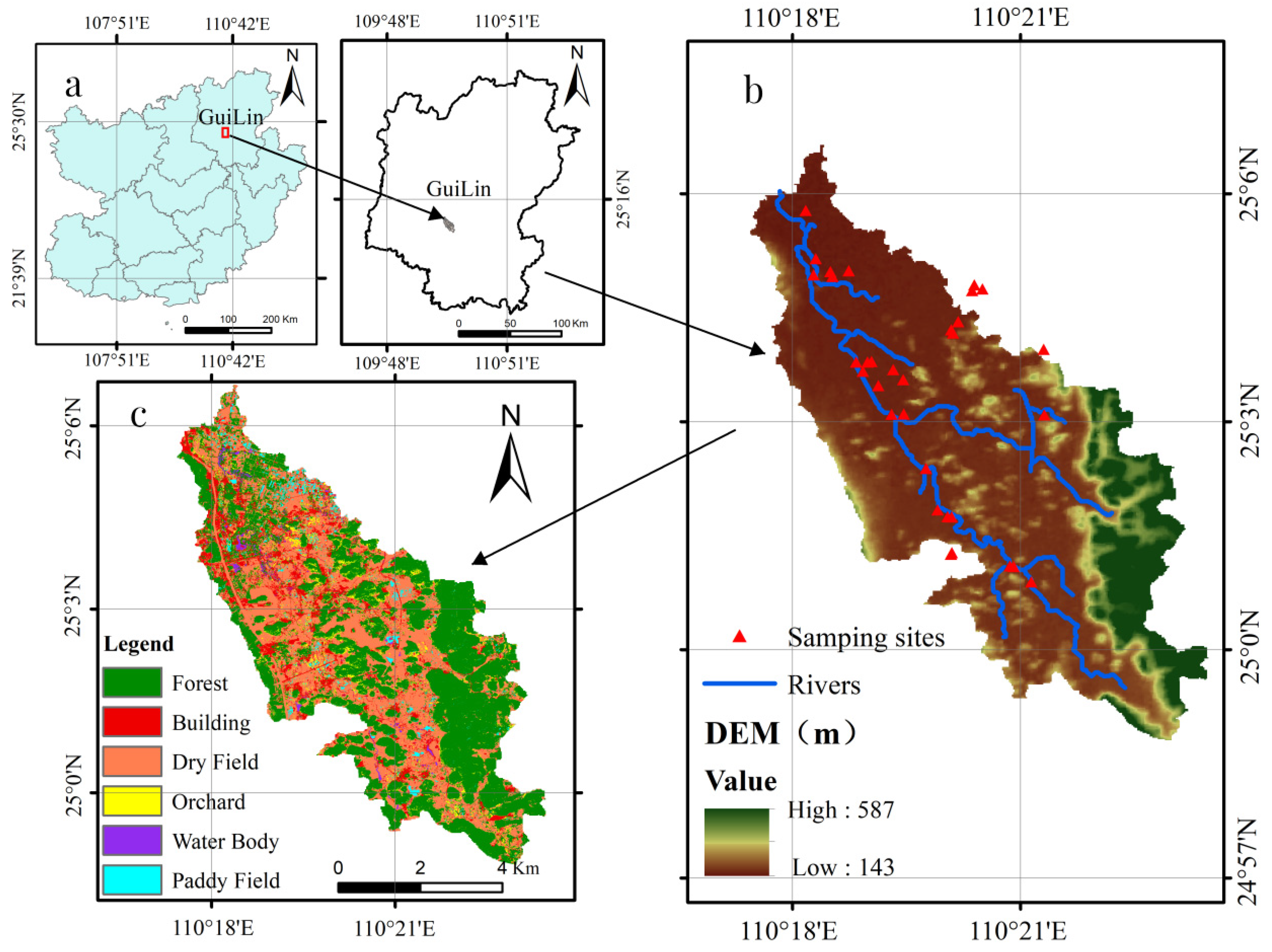
2.1. Study Area

This study was carried out over a period of two years in the Yanshan River Basin (YRB), a small watershed of the Lijiang River Basin, Guilin, China (Figure 1). The Yanshan River is a secondary tributary of the Lijiang River, with a river length of 13 km and a basin area of 65.3 km2 (latitude 24°59′ N~25°7′ N and longitude 110°17′ E~110°22′ E). The region experiences rainy springs and summers, windy autumns, and occasional frost and snow in winter. January is the coldest month of the year, with temperatures around 7–9 °C, while July is the hottest month, averaging 28.3 °C. The area’s climate is significantly influenced by the seasonal monsoons, resulting in distinct wet and dry seasons. Rainfall begins to increase in April, marking the onset of the wet season, which lasts until September. During this period, rainfall ranges from 1200 to 2000 mm, accounting for approximately 75% of the annual total. Conversely, winters are relatively cold and dry, with minimal rainfall, leading to potentially intermittent flow in some rivers [31]. The region is characterized by a diverse array of soil types, predominantly comprising typical wetland soil and karst soils. According to the findings of the second national soil survey in China, the principal soil types identified in the area include limestone soil, red soil or red and yellow soil, marsh soil, and paddy soil.

2.2. Water Sampling and Water Quality Analysis

Water sampling sites at tributaries, ditches, and ponds were set up in the YRB from May 2021 to May 2023. The study period was divided into wet seasons (from April to September) and dry seasons (from October to March) based on the climatic conditions. Water samples were collected every 10 days during the wet seasons and monthly during the dry seasons on average. We selected the sampling points according to the following principles: (1) The sampling points had to be highly representative, effectively reflecting the water conditions across the entire basin, and had to cover the basin comprehensively. (2) Priority had to be given to sampling agricultural non-point source pollution areas. (3) The selection of sampling points also had to consider convenience.
Dissolved oxygen (DO), pH, and electrical conductivity (EC) were measured on-site using a portable multi-parameter water quality analyzer (556 MPS Handheld Multiparameter Instrument; YSI Group, Davis, CA, USA). Water samples were collected at a depth of 0–20 cm below the water surface. A 500 mL plastic bottle was rinsed twice with the water to be sampled before each sample was taken. The samples (500 mL) were then collected and immediately transported to the laboratory for further analysis, where they were divided into two parts for water quality testing. The first part of each water sample was used to analyze the concentrations of TP and TN. The second part was treated by using vacuum filtration with a 0.45 μm acetate fiber membrane to isolate and analyze the dissolved constituents (NH4+-N and NO3-N), the concentrations of which were measured with standard analytical methods.
Water quality assessment is crucial to understanding and managing the quality of the water environment [32]. By using the single-factor pollution index, the comprehensive pollution index, and the pollution load ratio index methods, water quality can be evaluated comprehensively [32,33].
p i = c i c i 0
Among the options, DO was adopted, as p i = c i 0 / c i .
p m = p i max 2 + p i e v e 2 2
p t = 1 n p i
Q i = p i p t × 100 %
where Pi is the single-factor pollution index of pollutant i, Ci is the measured value of pollutant i, and Ci0 is the limit standard value of water pollution (taken as the standard value of class III according to the Surface Water Environmental Quality Standard [34] (GB3838-2002 Environmental quality standards for surface water in China, 2002): p ≤ 1 means that the water body examined is not polluted, while p > 1 indicates that the water is polluted, with a larger value indicating more significant pollution). Pm is the comprehensive pollution index, Pimax the maximum value of the single-factor pollution index, Pieve the average value of single-factor pollution indices, Pt the sum of single-factor pollution indices, and Qi the pollution load ratio for pollutant i.
Water quality was classified into five grades based on the comprehensive pollution index (Table 1).

2.3. Characterization of Landscape Patterns

In this study, landscape patterns were characterized on two scales: landscape composition and configuration. The former focused on the proportions of land-use areas and the latter on landscape indices.

2.3.1. Classification of Land Use in the YRB

A geographic information system (GIS) is a powerful tool used for managing, analyzing, and presenting geospatial data and related information [35], which is essential in fields such as urban planning and environmental protection [36]. Combined with remote sensing technology, remote sensing images obtained with GF-2 in 2018 at a resolution of 0.8 m × 0.8 m were used for land-use classification. Radiation calibration, atmospheric correction, and image cutting were performed in ENVI to reduce spectral differences and highlight target objects. Land-use types were then classified based on training samples estimated with field surveys by using support vector machines. Land use was categorized into forest, cultivated land, building, orchard, and water body (Figure 2). In order to analyze the spatial distributions of these land-use types, the YRB was divided into 21 sub-watersheds in ArcGIS based on DEM data with a spatial resolution of 5 m and a water system map (Figure 2). Based on the DEM data, the elevation distribution of the basin was extracted with the GIS, and the basin was subdivided into upper, middle, and lower reaches. This division was determined based on a combination of factors, including field surveys and measured velocity, as depicted in Figure 2.

2.3.2. Selection and Calculation of Landscape Indices

The landscape configuration indices included patch density (PD), largest patch index (LPI), percent of landscape (PLAND), edge density (ED), perimeter area fractal dimension (PAFRAC), and aggregation index (AI), as shown in Table 2. The landscape indices in the YRB were calculated with Fragstats3.3 (Kevin McGarigal et al., Oregon State University).

2.4. Statistical Analysis

The non-parametric Mann–Whitney U test was adopted to test the time differences of the water quality indicators. Spearman correlation analysis and redundancy analysis (RDA) were performed to examine the relationships between landscape patterns and water quality.

3. Results

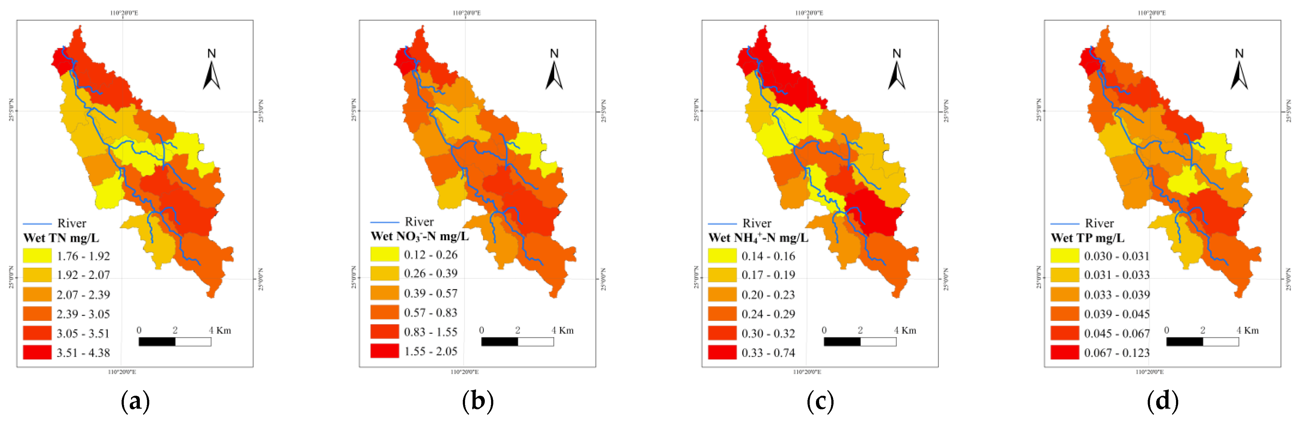
3.1. Nitrogen and Phosphorus Pollution of Water Bodies in the YRB

As shown in Figure 3, the average concentration of TN was 2.91 ± 1.01 mg/L, with the average values in the dry seasons being higher than those in the wet seasons. The average concentration of NO3-N (1.10 ± 0.43 mg/L) was higher than that of NH4+-N (0.24 ± 0.02 mg/L) during the study period, and, similar to TN, the concentrations of these pollutants in the dry seasons were significantly higher (p < 0.05) than those in the wet seasons. The concentrations of TP in this study ranged from 0.02 to 0.39 mg/L, with an average of 0.05 ± 0.004 mg/L; unlike NH4+-N and NO3—N, the average concentrations of TP were higher in the wet seasons than in the dry seasons. Regarding the average concentrations of TN, however, there were no significant differences between the dry and wet seasons (p > 0.05). Overall, nitrogen pollution was more severe during the dry seasons. The values of pH and EC were 7.77~9.10 and 244.38~488.42 S/m, respectively, and were significantly higher in the wet seasons, while the concentrations of DO were significantly higher in the dry seasons, varying between 3.98 and 9.13 mg/L (Figure 3).
As shown in Figure 4, water quality varied significantly among sub-watersheds, with greater differences being observed in the wet seasons. The average concentrations of TN fluctuated across the YRB (Figure 4). In the dry seasons, TN pollution was more significant in the upper and downstream sub-watersheds. Sub-watershed 1 exhibited the most severe TN pollution (6.13 mg/L), while the average TN concentration in sub-watershed 15 was the lowest (1.07 mg/L). In the wet seasons, TN pollution was more significant in middle and downstream sub-watersheds, with the highest average concentration of TN (4.38 mg/L) in sub-watershed 1 and the lowest average TN concentration (1.77 mg/L) in sub-watershed 19. The average concentrations of NO3-N in sub-watershed 2 were the highest in both the dry and wet seasons. The average concentrations of NO3-N in sub-watershed 15 (0.33 mg/L) and sub-watershed 17 (0.53 mg/L) were the lowest in the wet and dry seasons, respectively. NH4+-N pollution in the middle sub-watersheds was more severe, while it was relatively low in the upstream sub-watersheds. The average concentrations of NH4+-N in sub-watershed 1 (0.74 mg/L) and sub-watershed 17 (0.46 mg/L) were the highest in the wet and dry seasons, respectively. The average concentrations of TP in the downstream sub-watersheds were significantly higher than those in the upper and middle sub-watersheds during the study period.
Table 3 presents the single-factor pollution index, the comprehensive pollution index, and the pollution load ratio of water quality in the YRB. The single-factor pollution index of TN in the dry seasons ranged from 1.07 to 6.13, and its range was smaller in the wet seasons (1.77~4.38). TN exhibited the highest indices, indicating a significant contribution to pollution in the YRB. TN in sub-watershed 1 consistently displayed the largest single-factor pollution index in both season types, suggesting a higher level of TN pollution. The pollution indices of NH4+-N in the YRB were all less than 1, contributing little to nitrogen pollution. In the dry seasons, the single-factor pollution indices of TP were less than 1, except in sub-watershed 1, indicating less pollution by phosphorus in the YRB. The single-factor pollution indices of DO in the YRB were less than 1, suggesting less pollution by organic matter. The comprehensive pollution index in sub-watershed 2 was the highest, followed by upstream sub-watershed 19. Overall, the water quality in the YRB during the study period was lower than the value of class III according to the Surface Water Environmental Quality Standard (GB3838-2002), with the most severe pollution being downstream. The TN pollution load ratio was found to be remarkably high, 67.97%, indicating that TN was the main pollutant in the YRB.

3.2. Landscape Types of Different Sub-Watersheds in the YRB

As shown in Figure 1, the main land-use types in the YRB are forest and cultivated land, with the area of the former accounting for the largest proportion (46%), followed by the area of cultivated land (paddy field and dry land, 37%). Moreover, the proportions of building, orchard (mainly citrus orchards), and water body areas account for 11%, 5%, and 1% of the total area, respectively. The proportions of forest area decrease from upstream to downstream; the average proportion in sub-watershed 14 is the highest (89%), followed by that in sub-watershed 9 in the middle reaches (78.9%), while the average proportion of forest area in sub-watershed 6 is the lowest (29%). Cultivated land is uniformly distributed in the YRB (Figure 2). The proportion of cultivated land area in sub-watershed 8 is the highest (51.2%), followed by that in sub-watershed 15 (43.7%), while the proportion in sub-watershed 14 is the lowest (Figure 5). The proportions of building land area increase from upstream to downstream (Figure 2), and the proportions of building area in sub-watersheds 5 and 1 are the largest, accounting for 27.1% and 19.9%, respectively. The water area in the YRB has the smallest share, 1.2% on average, and the proportion of water area downstream is the largest (1.8%).

3.3. Landscape Indices in Sub-Watersheds of the YRB

The results of the landscape configuration indices in the sub-watersheds are displayed in Figure 6. The LPI represents the spatial configuration and dominance of land-use types, reflecting the intensity of the interference of human activity in a watershed. The LPI gradually decreases from upstream to downstream in the YRB, indicating that the intensity of human activity gradually increases from upstream to downstream. The LPI has its lowest value in sub-watershed 19, which is mainly covered by forest, while the LPI in sub-watershed 5, which is mainly covered by building land, is the highest. The distribution of the PD is similar to that of the LPI, indicating greater landscape fragmentation downstream. The ED, PAFRAC, and AI reflect the complexity of the landscape, and larger values indicate more complex landscape. All of these indicators increase from upstream to downstream, showing that the landscape downstream is more complex due to more intense human activity.

3.4. Relationships between Water Quality and Landscape Patterns

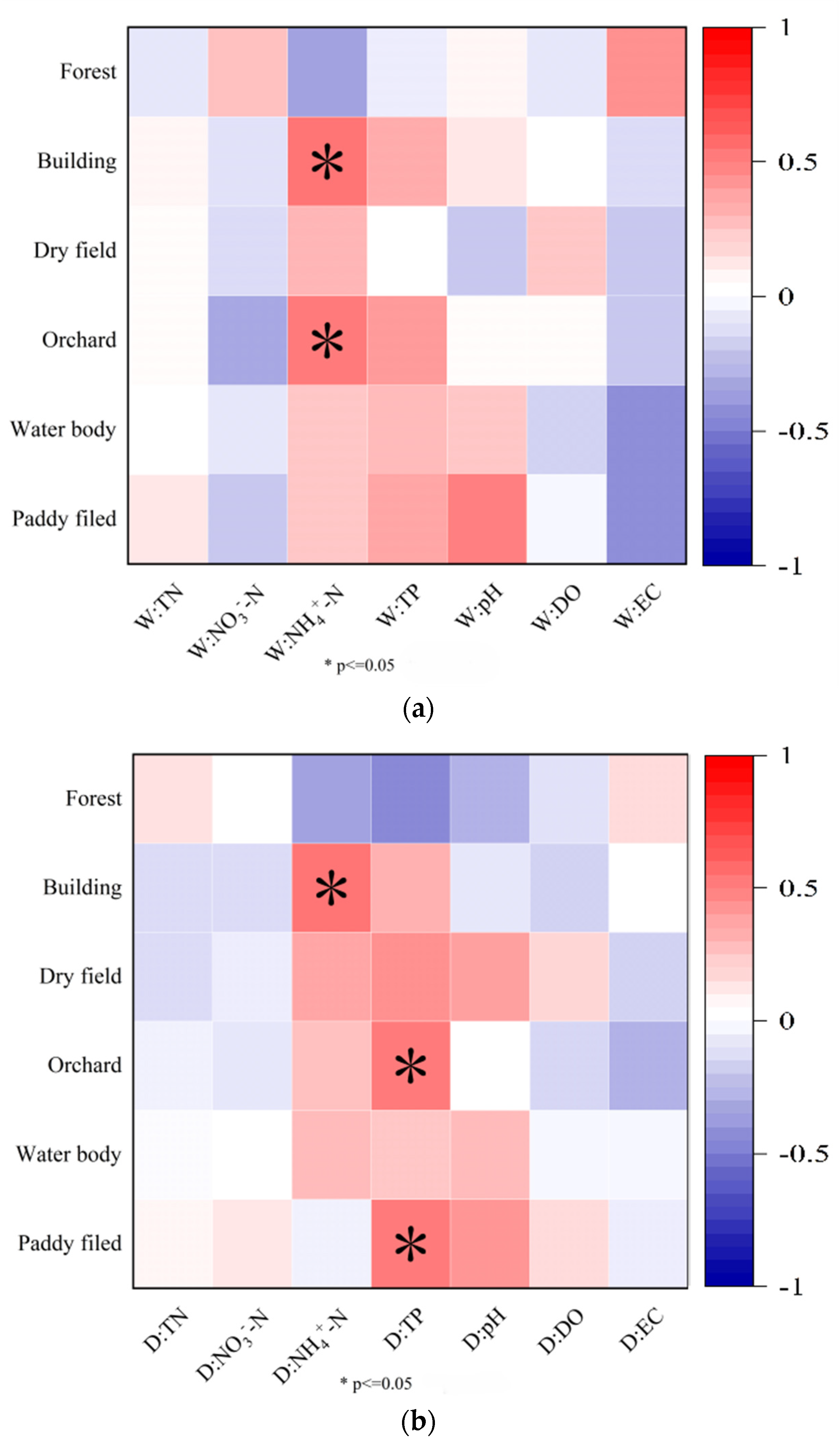
3.4.1. Correlations between Water Quality and Landscape Composition Indices

As shown in Figure 7, the TN concentrations did not exhibit significant correlations with the landscape composition indices during the study period. In the wet seasons, the NO3-N concentrations exhibited a negative correlation with the proportion of orchard area, while they showed a positive correlation with the proportion of forest area (p < 0.05). In contrast, the NO3-N concentrations were negatively correlated with the proportion of orchard area in the dry seasons (p < 0.05). The NH4+-N concentrations showed positive correlations with the proportion of building and orchard areas in the wet seasons and a negative correlation with the proportion of forest area in the dry seasons (p < 0.05). The TP concentrations displayed a positive correlation with the cultivated land area in the wet seasons, while they showed a negative correlation with the forest area (p < 0.05).

3.4.2. Relationships between Water Quality and Landscape Configuration Indices

As shown in Figure 8, the TN concentrations were positively correlated with AI_building-land and PAFRAC_orchard (p < 0.05) and negatively correlated with AI_forest, PAFRAC_paddy-field, and PAFRAC_water-body in the wet seasons, while they did not show significant correlations with the landscape configuration indices in the dry seasons. In the wet seasons, the NO3-N concentrations showed negative correlations with the LPI (p < 0.01) and ED (p < 0.05) of the water body area; however, they were not significantly correlated with landscape configuration in the dry seasons. The NH4+-N concentrations showed positive correlations with LPI_orchard (p < 0.01), PAFRAC_forest (p < 0.01), PD_building-land (p < 0.01), and LPI_building-land (p < 0.05) in the wet seasons; in the dry seasons, they were positively correlated with the landscape configuration indices of the building land area (p < 0.05).
The TP concentrations in the dry seasons were greatly influenced by the landscape configuration indices of the forest and orchard areas and were positively correlated with the LPI, ED, and PAFRAC of the forest area; the PD, LPI, PLAND, and ED of the orchard area; and LPI_building-land. The TP concentrations in the dry seasons were negatively correlated with AI_forest; however, those in the wet seasons were not significantly correlated with the landscape configuration indices, as shown in Figure 8.
In the dry seasons, EC was negatively correlated with AI_orchard (p < 0.05). In the wet seasons, the landscape configuration indices played more important roles in EC, which was positively correlated with LPI_forest (p < 0.01) and AI_forest (p < 0.05) and negatively correlated with ED_dry-land, LPI_water-body, ED_water-body, and ED_paddy-field (p < 0.05). In the wet seasons, pH was negatively correlated with PLAND_dry-land. However, the concentrations of NO3-N and TN and DO and the pH in the dry seasons, as well as the concentrations of TP and DO in the wet seasons, were not significantly correlated with the landscape configuration indices.

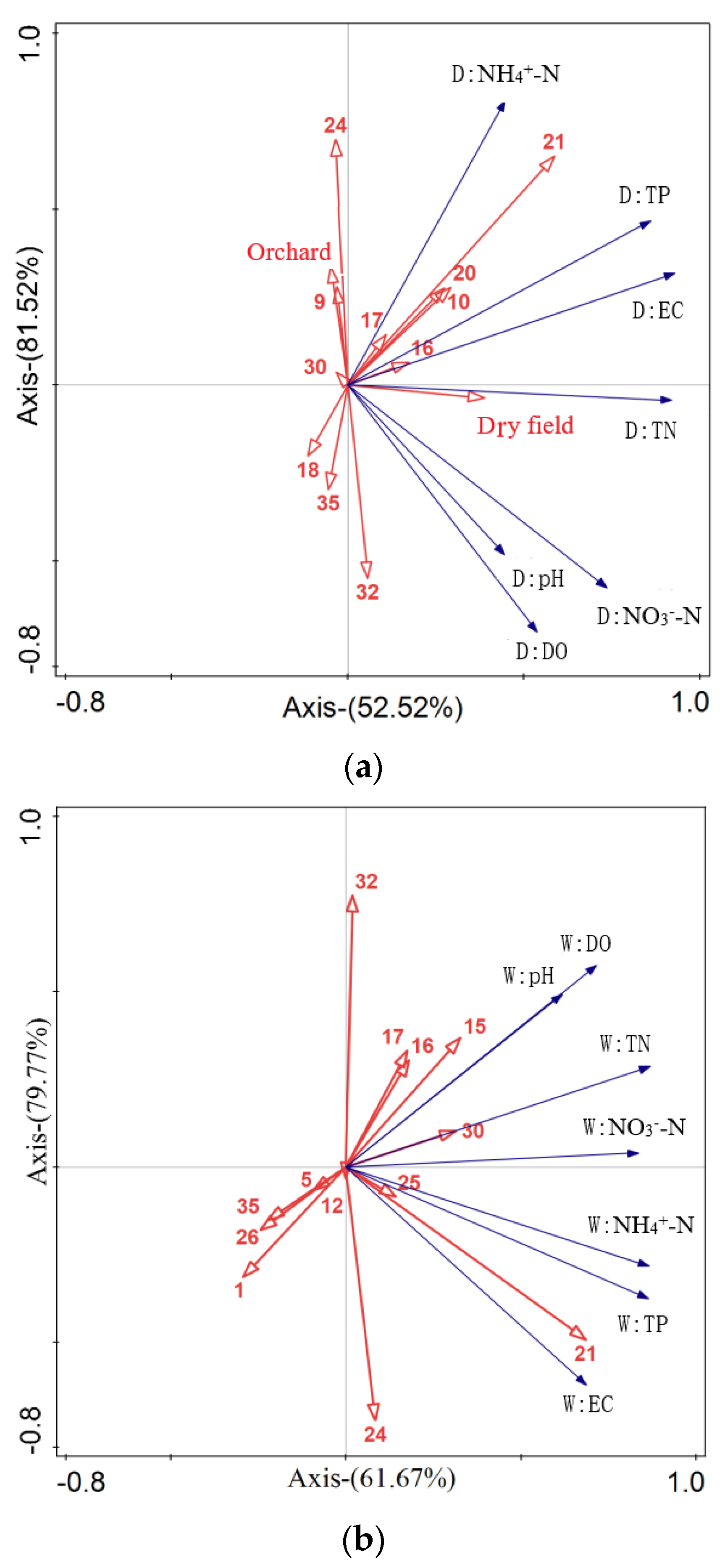
3.4.3. Contributions of Landscape Pattern Features to Water Quality in the YRB

As shown in Table 4, 52.5% and 29.0% of the variations in water quality were explained by the landscape pattern features of the first and second axes during the dry seasons, respectively. In the dry seasons, LPI_building-land (30.8%), AI_building-land (23.3%), PD_building-land (8.9%), and dry field (4.4%) were the main landscape configuration indices affecting water quality, while in the wet seasons, LPI_building-land (34.3%), AI_building-land (23.8%), and ED_forest (12.1%) were the most important explanatory landscape configuration indices for water quality.
As shown in Figure 9, the arrow lengths for the water quality indicators are long and closely grouped, signifying the substantial influence of the landscape composition and configuration indices on water quality. In the dry seasons, the concentrations of TN showed a significant positive correlation with the ratio of cultivated land area, while the concentrations of NO3-N and DO and the pH demonstrated negative correlations with AI_building-land, orchard area, and LPI_orchard. The concentrations of TP and NH4+-N exhibited positive correlations with the LPI and AI of the building land area, as reflected by the longest arrow length. In the wet seasons, all the water quality indicators displayed negative relationships with ED_forest, PD_water-body, PAFRAC_cultivated land, LPI_building-land, and AI_building-land. Specifically, the concentrations of NH4+-N and TP exhibited significant positive correlations with LPI_building-land (p < 0.05), and the values of TN, NO3-N, pH, and DO demonstrated positive associations with the LPI, ED, and PAFRAC of cultivated land (p > 0.05).

4. Discussion

4.1. Influencing Factors of Seasonal Variations in Water Quality

Nitrogen pollution in the YRB was the most significant during the dry seasons, in line with previous studies [37,38]. The comprehensive pollution indices in the dry seasons were generally greater than those in the wet seasons and increased with the increase in the proportions of building and cultivated land areas and with the decrease in the proportion of forest area. Moreover, nitrogen pollution in the lower reaches was significantly more severe than in the middle and upper reaches, and the deterioration of water quality was particularly pronounced in the dry seasons. Specifically, the average concentrations of TN in sub-watershed 1 at the outlet of the YRB, where the proportion of building land and dry field accounted for 53.3%, were the highest in the dry seasons (Figure 4).
During the study period, TP pollution in the basin was relatively low, with the sub-basin exhibiting the highest concentration of TP [39]. Seasonal runoff changes significantly impact the concentrations of nitrogen and phosphorus pollutants by washing them into aquatic ecosystems [40]. Point source pollution and rainy season runoff can modify how landscape composition and configuration affect water quality in different seasons. Previous studies have shown that urban areas are the main sources of point source pollutants, with residential area pollution dominating pollutant export during the dry season [41,42], leading to the strong influence of landscape composition and landscape configuration of building land on water quality in the dry season [43]. Increased rainfall during the rainy season leads to frequent rainfall and runoff, which can dilute and transport pollutants, reducing their concentration. This process results in the comprehensive pollution index being generally higher during the dry season, compared with the rainy season [44]. Additionally, the lush vegetation growth in the rainy season helps reduce soil erosion and pollutant loss, further contributing to the lower comprehensive pollution index during this period. The YRB experiences a subtropical monsoon climate, which is hot and rainy in summer and warm and dry in winter. In dry seasons, nitrogen is more likely to accumulate in water body ecosystems because of slow or intermittent runoff flow.

4.2. Relationship between Landscape Composition and Water Quality Indicators

The heterogeneity of landscape composition reflects non-spatial structural characteristics, mainly including the types and area proportion of land use, altering the retention and absorption of pollutants [21,23]. Therefore, the relationships between water quality and different landscape composition patterns in the YRB showed obvious differences.
The building land type had significant impacts on water quality during the study period, and there was a significant positive correlation between NH4+-N concentrations and the proportion of building land area (Figure 7). The results of monitored water quality show that the sub-watersheds with high NH4+-N concentrations were mostly distributed in the middle and lower reaches, especially at the outlet (Figure 4). The building land area in these sub-watersheds accounts for a relatively high proportion, and the domestic pollutants discharged from them become an important source of pollution in sub-watersheds. In addition, the increase in impervious area of building land also accelerates the flow of pollutants into water bodies along with rainfall runoff. The orchards had positive effects on the NH4+-N and TP concentrations, with significant effects on the former in the wet seasons and on the latter in the dry seasons (Figure 7). This might be related to the characteristics of fertilization, ground cover, and terrain of orchards. Previous researchers found that nitrogen and phosphorus in orchard runoff were mainly dissolved nitrogen and particle-derived phosphorus [45]. According to the investigation, the orchards in the study area were mainly supplemented with ammonia fertilizer in wet seasons, and ammonia loss was promoted by rainfall runoff. The coverage rate of vegetation (grass) on the ground of the orchard was low, with the ground being nearly bare in dry seasons. Under the erosion of rainfall and runoff, surface soil particles were more likely to produce phosphorus loss. Moreover, the orchard had a well-defined slope, and the lost nitrogen and phosphorus could easily enter the surrounding water.
It is worth noting that, although previous studies have shown that water quality deterioration is significantly positively correlated with cultivated land coverage [46,47,48], only paddy field had a positive effect on the TP concentrations in the dry seasons and did not significantly affect other water quality indices. This indicates that the ratio of cultivated land area (coverage rate) in the study area could not reflect the impacts on water quality; thus, the effects of cultivated land on water quality needed to be clarified. Previous studies have shown that forest, as the “sink” for N and P pollution in a basin, has positive effects on the purification of surface water [49]. In this study, forest had negative effects on the concentrations of NH4+-N, TN, and TP in the wet seasons; however, these effects were not significant. In this study, most forest was concentrated in the upper reaches and at the edge of the basin, so it was difficult for it to play a role in pollution source interception and purification. Moreover, the distribution of forest in the middle and lower reaches was scattered, so it was difficult for it to form an effective interception zone. Rivers, ditches, and ponds in the basin, as places for the transport and (temporary) storage of pollutants, can change the concentrations and composition of N and P pollutants through various effects. However, due to the small proportion of water bodies in this study (Figure 5) and poor connectivity, the water bodies did not show significant influences on water quality.

4.3. Relationship between Landscape Configuration Indices and Water Quality

To further reveal the impacts of landscape patterns on water quality in the basin, the influences of the landscape indices of different land-use types in the dry and wet seasons were analyzed, and the results show that the landscape indices of orchards, building land, and forest areas had more prominent impacts on surface water quality (Figure 8).
Compared with the orchard area ratio, the landscape configuration indices of the orchard land-use type were more closely related to surface water quality. The PD, PLAND, ED, LPI, and PAFRAC of the orchard area were positively correlated with the concentrations of TP, NH4+-N, and TN in the wet seasons, while the AI was significantly negatively correlated with EC in the dry seasons (Figure 8). The results indicate that larger orchard landscape density, maximum patch area, and patch proportion contributed to higher N and P concentrations in the water body area. The orchards in the study area showed a characteristically scattered distribution within the YRB, but were concentrated near water bodies (rivers) (Figure 5), and landscape features such as area size and shape changed greatly. Runoff and pollutants generated from orchards easily enter downstream water bodies, negatively affecting water quality.
The landscape indices of the building land area had significant impacts on the water quality indicators (Figure 8). The LPI of the building land area had a significant positive correlation with NH4+-N, dry season TP, and wet season TN during the study period. The LPI reflects the dominant landscape type in the region, and its change can reflect the direction and intensity of human activity to a certain extent. For the building land type, the higher the LPI value, the greater the degree of human activity interference [50]. The greater the patch dominance of building land area in the study area, the easier it was for a large number of nitrogen and phosphorus pollutants to be discharged, which is not conducive to surface water quality. Therefore, the LPI of building land area had the highest weight in the assessment of water quality (Table 4). In the study period, PD, NH4+-N, PLAND, ED, and AL were significantly positively correlated with the NH4+-N concentration in the dry seasons, further indicating that the more concentrated the building land distribution, the greater the density, the better the connectivity between patches, and the closer the relationship with other landscapes, the more likely it is that there is NH4+-N pollution in the surrounding water bodies.
The average concentrations of TP in the dry seasons and NH4+-N in the wet seasons were significantly positively correlated with the LPI and PAFRAC of the forest area, unlike the proportion of forest area. The forest landscape area in the middle and lower reaches of the basin is complex in shape and highly fragmented, as well as combined with cultivated land and orchards (Figure 5). Due to human interference, the function of being a pollutant “sink” is weak or even absent, which is conducive to the accumulation of runoff pollutants downstream. The forest AI has a negative correlation with TP in the dry seasons and a positive correlation with EC in the wet seasons. If the aggregation of forest area increases, a continuous pollutant interception and purification zone can form, which may lead to reduced phosphorus loss.
The proportion of water area in the study basin is small, but the LPI and ED of the water area has a significant negative correlation with the NO3-N and EC concentrations in the wet seasons. Natural rivers, artificial ditches, and ponds, which are widely distributed and scattered in the YRB, directly transport and store the runoff and pollutants from the surrounding landscapes, and remove N pollutants through biochemical and physical reactions (especially denitrification) [51]. A single water body with a larger area enhances the hydrological connectivity with the surrounding landscape, which strengthens its ability to collect, store, and reduce pollutants. Similarly, the PAFRAC and ED of the paddy field area also has significant negative effects on the NO3-N concentrations in the wet seasons. Intermittent irrigation, making full use of rainfall, is generally adopted in paddy fields, and the bunds can reduce drainage runoff and the accompanying N and P pollutants. During the study period, the monitoring of paddy water showed that the average concentration of NO3-N (0.492 mg/L) was significantly lower than those of most water bodies, with paddy fields, i.e., constructed wetlands, functioning as “sinks” for NO3-N. Therefore, the shape of paddy field patches is closely related to other landscape types with complex shapes and decreases NO3-N pollution in the wet seasons under appropriate human intervention.

5. Conclusions

In this study, water quality was evaluated for the wet and dry seasons, and the relationship between water quality and landscape characteristics at two scales (i.e., landscape composition and landscape configuration) was explored in the Yanshan River Basin, Guilin, China, by combining remote sensing technology and landscape ecology. During the study period, the average concentrations of nitrogen and phosphorus pollutants were lower in the wet seasons than in the dry seasons. Moreover, TN was the primary pollutant source. The correlation analysis between the landscape composition indices and water quality showed that a larger proportion of forest area could decrease TN, NH4+-N, NO3-N, and TP pollution, while larger proportions of building, orchard, and cultivated land areas increased NO3-N and TP pollution. From the perspective of landscape configuration indices, the concentrations of nitrogen were significantly affected by the indices of the building land area, while the concentrations of TP were greatly affected by the indices of the forest and orchard areas. Moreover, the correlations between these indices and water quality were greater in the wet seasons than in the dry seasons. Furthermore, the landscape configuration indices were more effective in explaining water quality changes than were the landscape composition indices.

Author Contributions

Conceptualization, B.X.; Software, Z.F.; Investigation, P.X., C.Z. and J.H.; Writing—original draft, Z.F.; Writing—review & editing, Z.F., R.F., B.X., Q.X. and J.D.; Funding acquisition, B.X. All authors have read and agreed to the published version of the manuscript.

Funding

This work was supported by the Natural Science Foundation of Guangxi, China (grant numbers 2022GXNSFBA035614 and 2024GXNSFAA010519), and the Science and Technology Major Project of Guangxi, China (grant number GuikeAB22035075), and was supported in part by the Foundation of Key Laboratory of Guangxi (grant number Guikeneng21201Z011) and the Guilin University of Technology Foundation (grant number GUTQDJJ2019026).

Data Availability Statement

Data are contained within the article.

Conflicts of Interest

The authors declare that they have no known competing financial interest or personal relationships that could have appeared to influence the work reported in this paper.

Abbreviations

YRBYanshan River Basin
NPSNon-point source
WWet season
DDry season

References

  1. De Oliveira, L.M.; Maillard, P.; de Andrade Pinto, E.J. Application of a land cover pollution index to model non-point pollution sources in a Brazilian watershed. Catena 2017, 150, 124–132. [Google Scholar] [CrossRef]
  2. Sun, X.; Zhang, H.; Zhong, M.; Wang, Z.; Liang, X.; Huang, T.; Huang, H. Analyses on the Temporal and Spatial Characteristics of Water Quality in a Seagoing River Using Multivariate Statistical Techniques: A Case Study in the Duliujian River, China. Int. J. Environ. Res. Public Health 2019, 16, 1020. [Google Scholar] [CrossRef] [PubMed]
  3. Yue, Y.; Cheng, H.; Yang, S.T.; Hao, F. Estimation and evaluation of non-point source pollution load in Songhua River Basin. Sci. Geogr. Sin. 2007, 27, 231–236. (In Chinese) [Google Scholar]
  4. Ouyang, W.; Skidmore, A.K.; Toxopeus, A.G.; Hao, F. Long-term vegetation landscape pattern with non-point source nutrient pollution in upper stream of Yellow River basin. J. Hydrol. 2010, 389, 373–380. [Google Scholar] [CrossRef]
  5. Wu, J.; Lu, J. Landscape patterns regulate non-point source nutrient pollution in an agricultural watershed. Sci. Total Environ. 2019, 669, 377–388. [Google Scholar] [CrossRef] [PubMed]
  6. Hassan, Z.U.; Shah, J.A.; Kanth, T.A.; Pandit, A.K. Influence of land use/land cover on the water chemistry of Wular Lake in Kashmir Himalaya (India). Ecol. Process. 2015, 4, 9. [Google Scholar] [CrossRef]
  7. Dai, X.; Zhou, Y.; Ma, W.; Zhou, L. Influence of spatial variation in land-use patterns and topography on water quality of the rivers inflowing to Fuxian Lake, a large deep lake in the plateau of southwestern China. Ecol. Eng. 2017, 99, 417–428. [Google Scholar] [CrossRef]
  8. Zhang, F.; Chen, Y.; Wang, W.; Jim, C.; Zhang, Z.; Tan, M.L.; Liu, C.; Chan, N.; Wang, D.; Wang, Z.; et al. Impact of land-use/land-cover and landscape pattern on seasonal in-stream water quality in small watersheds. J. Clean. Prod. 2022, 357, 131907. [Google Scholar] [CrossRef]
  9. Wang, R.; Xu, T.; Yu, L.; Zhu, J.; Li, X. Effects of land use types on surface water quality across an anthropogenic disturbance gradient in the upper reach of the Hun River, Northeast China. Environ. Monit. Assess. 2013, 185, 4141–4151. [Google Scholar] [CrossRef]
  10. Li, H.; Huang, Y.; Guo, W.; Hou, H.; Fan, M.; Qi, X.; Jia, P.; Guo, Q. Effects of land use and spatial pattern on water quality in Hehuang Valley at different spatial and temporal scales. Environ. Sci. 2022, 43, 4042–4053. (In Chinese) [Google Scholar]
  11. Townsend, C.R.; Dolédec, S.; Norris, R.; Peacock, K.; Arbuckle, C. The influence of scale and geography on relationships between stream community composition and landscape variables: Description and prediction. Freshw. Biol. 2010, 48, 768–785. [Google Scholar] [CrossRef]
  12. Turner Goigel, M. Landscape Ecology: The Effect of Pattern on Process. Annu. Rev. Ecol. Syst. 1989, 20, 171–197. [Google Scholar] [CrossRef]
  13. Beckert, K.A.; Fisher, T.R.; O’Neil, J.M.; Jesien, R.V. Characterization and Comparison of Stream Nutrients, Land Use, and Loading Patterns in Maryland Coastal Bay Watersheds. Water Air Soil Pollut. 2011, 221, 255–273. [Google Scholar] [CrossRef]
  14. Uriarte, M.; Yackulic, C.B.; Lim, Y.; Arce-Nazario, J.A. Influence of land use on water quality in a tropical landscape: A multi-scale analysis. Landsc. Ecol. 2011, 26, 1151–1164. [Google Scholar] [CrossRef] [PubMed]
  15. Stryjecki, R.; Zawal, A.; Stępień, E.; Buczyńska, E.; Buczyński, P.; Czachorowski, S.; Szenejko, M.; Śmietana, P. Water mites (Acari, Hydrachnidia) of water bodies of the Krąpiel River valley: Interactions in the spatial arrangement of a river valley. Limnology 2016, 17, 247–261. [Google Scholar] [CrossRef]
  16. Teixeira, Z.; Marques, J.C. Relating landscape to stream nitrate-N levels in a coastal eastern-Atlantic watershed (Portugal). Ecol. Indic. 2016, 61, 693–706. [Google Scholar] [CrossRef]
  17. Rajaei, F.; Sari, A.E.; Salmanmahiny, A.; Delavar, M.; Bavani, A.; Srinivasan, R. Surface drainage nitrate loading estimate from agriculture fields and its relationship with landscape metrics in Tajan watershed. Paddy Water Environ. 2017, 15, 541–552. [Google Scholar] [CrossRef]
  18. Valjarević, A. GIS-Based Methods for Identifying River Networks Types and Changing River Basins. Water Resour. Manag. 2024, 221, 255–273. [Google Scholar] [CrossRef]
  19. Griffith, J.A. Geographic Techniques and Recent Applications of Remote Sensing to Landscape-Water Quality Studies. Water Air Soil Pollut. 2002, 138, 181–197. [Google Scholar] [CrossRef]
  20. Fan, Z.; Liu, J.; Yue, Z.; Feng, K.; Wang, Q.; Li, F.; Tu, Z. Spatial heterogeneity of water quality and its response to land use in Puhe River Basin. Chin. J. Ecol. 2018, 37, 1144–1151. (In Chinese) [Google Scholar]
  21. Goldstein, R.M.; Carlisle, D.M.; Meador, M.R.; Short, T.M. Can basin land use effects on physical characteristics of streams be determined at broad geographic scales? Environ. Monit. Assess. 2007, 130, 495–510. [Google Scholar] [CrossRef]
  22. Zhang, J.J.; Gurkan, Z.; Rgensen, S.E. Application of eco-exergy for assessment of ecosystem health and development of structurally dynamic models. Ecol. Model. 2010, 221, 693–702. [Google Scholar] [CrossRef]
  23. Meneses, B.M.; Reis, R.; Vale, M.J.; Saraiva, R. Land use and land cover changes in Zêzere watershed (Portugal)—Water quality implications. Sci. Total Environ. 2015, 527–528, 439–447. [Google Scholar] [CrossRef] [PubMed]
  24. Ding, J.; Jiang, Y.; Liu, Q.; Hou, Z.; Liao, J.; Fu, L.; Peng, Q. Influences of the land use pattern on water quality in low-order streams of the Dongjiang River basin, China: A multi-scale analysis. Sci. Total Environ. 2016, 551–552, 205–216. [Google Scholar] [CrossRef]
  25. Shehab, Z.N.; Jamil, N.R.; Aris, A.Z.; Shafie, N.S. Spatial variation impact of landscape patterns and land use on water quality across an urbanized watershed in Bentong, Malaysia. Ecol. Indic. 2021, 122, 107254. [Google Scholar] [CrossRef]
  26. Guo, Y.; Li, S.; Liu, R.; Zhang, J. Relationship between landscape pattern and water quality of the multi-scale effects in the Yellow River Basin. J. Lake Sci. 2021, 33, 737–748. (In Chinese) [Google Scholar]
  27. Zhu, Y.; Wang, Y. Spatial scale effects of landscape pattern on water quality change in Yangcheng Lake Watershed. Bull. Soil Water Conserv. 2021, 41, 105–113. (In Chinese) [Google Scholar]
  28. Wei, P.; Lei, Q.; Ying, Z.; Xu, Q.; Du, X.; Luo, J.; An, M. Effect of landscape pattern on river water quality under different regional delineation methods: A case study of Northwest Section of the Yellow River in China. J. Hydrol. Reg. Stud. 2023, 50, 101536. [Google Scholar] [CrossRef]
  29. Khan, H.H.; Khan, A.; Ahmed, S.; Perrin, J. GIS-based impact assessment of land-use changes on groundwater quality: Study from a rapidly urbanizing region of South India. Environ. Earth Sci. 2011, 63, 1289–1302. [Google Scholar] [CrossRef]
  30. Li, K.; Chi, G.G.; Wang, L.; Xie, Y.; Wang, X.; Fan, Z. Identifying the critical riparian buffer zone with the strongest linkage between landscape characteristics and surface water quality. Ecol. Indic. 2018, 93, 741–752. [Google Scholar] [CrossRef]
  31. Guilin, Y.; District Local Chronicles Compilation Committee. Yanshan Yearbook (2019); Thing-Bound Book Bureau: Beijing, China, 2019; Volume 11, pp. 1–2. [Google Scholar]
  32. Liu, S.; Lou, S.; Kuang, C.; Huang, W.; Chen, W.; Zhang, J.; Zhong, G. Water quality assessment by pollution-index method in the coastal waters of Hebei Province in western Bohai Sea, China. Mar. Pollut. Bull. 2011, 62, 2220–2229. [Google Scholar] [CrossRef] [PubMed]
  33. Qiao, G.; Zhou, Y.; Gu, Z.; He, J. Correlation between landscape pattern characteristics and water quality in pits and ponds in southern Jiangsu. Trans. Chin. Soc. Agric. Eng. 2021, 37, 224–234. (In Chinese) [Google Scholar]
  34. GB3838-2002; Environmental Quality Standards for Surface Water in China. Ministry of Ecology and Environment of People’s Republic of China: Beijing, China, 2002.
  35. Liu, S.H.; Wu, C.J.; Shen, H.Q. A GIS based Model of Urban Land Use Growth in Beijing. Acta Geogr. Sin. 2000, 55, 407–416. (In Chinese) [Google Scholar]
  36. Worese, A.T. Urban Layout Planning for African Cities by GIS Based Cellular Automata: Case of Ouagadougou, Burkina Faso; Wageningen University: Wageningen, The Netherlands, 2004. [Google Scholar]
  37. Zhu, G.W. Spatio-temporal distribution pattern of water quality in Lake Taihu and its relation with cyanobacterial blooms. Resour. Environ. Yangtze Basin 2009, 18, 439–445. (In Chinese) [Google Scholar]
  38. Liu, Z.; Wang, X.; Jia, S.; Mao, B. Multi-methods to investigate spatiotemporal variations of nitrogen-nitrate and its risks to human health in China’s largest fresh water lake (Poyang Lake). Sci. Total Environ. 2023, 863, 160975. [Google Scholar] [CrossRef]
  39. Yi, J.; Xu, F.; Gao, Y.; Xiang, L.; Mao, X. Variations of water quality of the major 22 inflow rivers since 2007 and impacts on Lake Taihu. J. Lake Sci. 2016, 28, 1167–1174. (In Chinese) [Google Scholar]
  40. Tian, L.; Zhu, X.; Wang, L.; Du, P.; Peng, F.; Pang, Q. Long-term trends in water quality and influence of water recharge and climate on the water quality of brackish-water lakes: A case study of Shahu Lake. J. Environ. Manag. 2020, 276, 111290. [Google Scholar] [CrossRef] [PubMed]
  41. Ye, Y.; He, X.; Chen, W.; Yao, J.; Yu, S.; Jia, L. Seasonal water quality upstream of Dahuofang reservoir, China—The effects of land use type at various spatial scales. Clean–Soil Air Water 2014, 42, 1423–1432. [Google Scholar] [CrossRef]
  42. Bu, H.M.; Meng, W.; Zhang, Y.; Wan, J. Relationships between land use patterns and water quality in the Taizi River basin, China. Ecol. Indic. 2014, 41, 187–197. [Google Scholar] [CrossRef]
  43. Cheng, X.; Song, J.; Yan, J. Influences of landscape pattern on water quality at multiple scales in an agricultural basin of western China. Environ. Pollut. 2023, 319, 120986. [Google Scholar] [CrossRef]
  44. Jia, Z.L.; Chang, X.; Duan, T.T.; Wang, X.; Wei, T.; Li, Y. Water quality responses to rainfall and surrounding land uses in urban lakes. J. Environ. Manag. 2021, 298, 113514. [Google Scholar] [CrossRef] [PubMed]
  45. Zhang, H.M.; Xu, Q.T.; Zhang, M.K. Application of different management measures to reduce runoff losses of nitrogen, phosphorus and copper from orchard in dense river network plain. Trans. Chin. Soc. Agric. Eng. 2014, 30, 132–138. (In Chinese) [Google Scholar]
  46. Evans, D.M.; Schoenholtz, S.H.; Wigington, P.J.; Griffith, S.M.; Floyd, W.C. Spatial and temporal patterns of dissolved nitrogen and phosphorus in surface waters of a multi-land use basin. Environ. Monit. Assess. 2014, 186, 873–887. [Google Scholar] [CrossRef] [PubMed]
  47. Dambeniece-Migliniece, L.; Veinbergs, A.; Lagzdins, A. The impacts of agricultural land use on nitrogen and phosphorus loads in the Mellupite catchment. Energy Procedia 2018, 147, 189–194. [Google Scholar] [CrossRef]
  48. Pärn, J.; Henine, H.; Kasak, K.; Kauer, K.; Sohar, K.; Tournebize, J.; Uuemaa, E.; Välik, K.; Mander, Ü. Nitrogen and phosphorus discharge from small agricultural catchments predicted from land use and hydroclimate. Land Use Policy 2018, 75, 260–268. [Google Scholar] [CrossRef]
  49. Doody, D.G.; Withers, P.J.; Dils, R.M.; McDowell, R.W.; Smith, V.; McElarney, Y.R.; Dunbar, M.; Daly, D. Optimizing land use for the delivery of catchment ecosystem services. Front. Ecol. Environ. 2016, 14, 325–332. [Google Scholar] [CrossRef]
  50. Lü, L.; Zhang, J.; Sun, C.; Wang, X.; Zheng, D. Landscape ecological risk assessment of Xi river Basin based on land-use change. Acta Ecol. Sin. 2018, 38, 5952–5960. (In Chinese) [Google Scholar]
  51. Wang, L.; Shang, S.; Liu, W.; Liu, W.; She, D.; Hu, W.; Liu, Y. Hydrodynamic controls on nitrogen distribution and removal in aquatic ecosystems. Water Res. 2023, 242, 120257. [Google Scholar] [CrossRef]
Figure 1. (a) Map showing the YRB location. (b) DEM and the water sampling sites in the YRB. (c) Land use in the YRB.
Water 16 02472 g001
Figure 2. The distribution of the upper, middle, and lower sub-watersheds in the YRB. Note: 1–21 refer to the numbers of the sub-basins.
Water 16 02472 g002
Figure 3. A comparison of water quality between wet and dry seasons in the YRB. Notes: Different letters above the plot boxes indicate significant differences at the 0.05 level; W: wet season; D: dry season.
Water 16 02472 g003
Figure 4. Spatial variations in water quality indicators in dry and wet seasons in sub-watersheds: (a) TN, (b) NO3-N, (c) NH4+-N, and (d) TP concentrations in wet seasons; (e) TN, (f) NO3-N, (g) NH4+-N, and (h) TP concentrations in dry seasons.
Water 16 02472 g004aWater 16 02472 g004b
Figure 5. The proportions of land-use areas in different sub-watersheds in the YRB. Note: 1–21 refer to the sub-basin identification number.
Water 16 02472 g005
Figure 6. Distributions of landscape configuration indices in the YRB: (a) LPI; (b) AI; (c) ED; (d) PD; (e) PAFRAC; and (f) PLAND.
Water 16 02472 g006
Figure 7. Correlations between water quality and landscape composition in the YRB. Correlations between landscape composition and water quality in wet seasons (a) and dry seasons (b).
Water 16 02472 g007
Figure 8. Correlations between water quality and landscape configuration indices in the YRB. Correlations between landscape configuration and water quality in the wet seasons (a) and dry seasons (b). 1: PD_forest; 2: LPI_forest; 3: PLAND_forest; 4: ED_forest; 5: PAFRAC_forest; 6: AI_forest; 7: PD_orchard; 8: LPI_orchard; 9: PLAND_orchard; 10: ED_orchard; 11: PAFRAC_orchard; 12: AI_orchard; 13: PD_dry-land; 14: LPI_dry-land; 15: PLAND_dry-land; 16: ED_dry-land; 17: PAFRAC_dry-land; 18: AI_dry-land; 19: PD_building-land; 20: LPI_building-land; 21: PLAND_building-land; 22: ED_building-land; 23: PAFRAC_building-land; 24: AI_building-land; 25: PD_water-body; 26: LPI_water-body; 27: PLAND_water-body; 28: ED_water-body; 29: PAFRAC_water-body; 30: AI_water-body; 31: PD_paddy-field; 32: LPI_paddy-field; 33: PLAND_paddy-field; 34: ED_paddy-field; 35: PAFRAC_paddy-field; 36: AI_paddy-field. * p ≤ 0.05; ** p ≤ 0.01.
Water 16 02472 g008aWater 16 02472 g008b
Figure 9. The correlations between water quality (represented by blue arrows) and landscape pattern features (represented by red arrows) in different seasons based on redundancy analysis (RDA): (a) wet and (b) dry seasons.
Water 16 02472 g009
Table 1. Water quality classification for the YRB.
GradeComprehensive Pollution IndexPollution Degree
1Pm ≤ 0.7Clean
20.7 < Pm ≤ 1.0Generally clean
31.0 < Pm ≤ 2.0 Slightly polluted
42.0 < Pm ≤ 3.0Moderately polluted
5Pm > 3.0Strongly polluted
Table 2. Parameters characterizing landscape patterns in this study.
Landscape Pattern ScaleNameDescription
Landscape composition indicesWater bodyWater body area ratio
Cultivated landCultivated land area ratio
BuildingBuilding area ratio
OrchardOrchard area ratio
ForestForest area ratio
Landscape configuration indicesPDNumber of patches per unit area (100 hm2)
LPIPercentage of the largest patch area of the total landscape area
PLANDPatch-area to total-area ratio
EDDirect reflection of the degree of landscape fragmentation
PAFRACComplexity of traits at different spatial scales
AIConnectivity between patches of each landscape type
Table 3. Results of water quality assessment in the YRB.
Wet Seasons
Sub-Watershed No.Single-Factor Pollution IndexComprehensive Pollution IndexSub-Watershed No.Single-Factor Pollution IndexComprehensive Pollution Index
TNNH4+-NTPDOTNNH4+-NTPDO
14.380.740.620.733.3010, 11, 122.390.270.190.791.81
23.930.290.210.722.92132.770.300.190.672.08
42.830.300.270.792.13143.050.160.160.932.29
52.750.280.220.882.08153.520.190.180.762.62
61.820.230.201.261.4317, 182.270.320.231.041.74
72.830.310.340.802.14191.770.160.290.871.36
82.270.210.160.921.73202.080.140.160.961.58
93.310.190.150.882.48211.920.150.220.761.46
Dry Seasons
16.130.601.890.604.6410, 11, 122.650.350.170.581.99
23.710.160.260.552.75132.780.170.180.592.07
44.030.090.190.552.97143.870.180.120.642.86
52.200.310.130.661.66151.590.210.250.581.22
62.410.210.140.851.8217, 182.990.460.210.742.25
73.000.150.200.662.24194.530.050.080.583.34
82.470.170.140.651.85202.520.130.140.611.88
91.070.090.180.660.83213.260.100.120.632.41
Table 4. Interpretation rates and contributions of landscape indices to water quality.
SeasonsExplained Variation (%)Explanatory Variables (Contribution %)
Axis 1Axis 2Axis 3Axis 4
Dry seasons52.581.591.596.9LPI_building-land (30.8%), AI_building-land (23.2%), PD_building-land (8.9%), and dry field (4.4%)
Wet seasons61.779.887.694.4LPI_building-land (34.3%), AI_building-land (23.8%), ED_forest (12.1%), ED_cultivated land (7.6%), and PLAND_arid (7%)
Disclaimer/Publisher’s Note: The statements, opinions and data contained in all publications are solely those of the individual author(s) and contributor(s) and not of MDPI and/or the editor(s). MDPI and/or the editor(s) disclaim responsibility for any injury to people or property resulting from any ideas, methods, instructions or products referred to in the content.

