Abstract
The area of Sia Kouanza in the Sahel of southwestern Niger is a potential location for expanding agriculture through irrigation with groundwater. Agriculture is key to supporting smallholders and promoting food security. As plans proceed, questions include how much water is available, how is groundwater replenished, many hectares to develop, and where to locate the wells. While these questions can be addressed with a model, it is difficult to find detailed procedures, especially when data are scarce. How can we use existing information to develop a model of a natural system where groundwater development will take place? We describe an approach that can be employed in data-scarce areas where similar questions are being asked. The approach includes setting details; conceptual model development; water balance; numerical code MODFLOW; model construction, calibration, and statistics; and result interpretation. Conceptual model component estimates are derived from field data: recharge, evapotranspiration, wetlands discharge, existing extraction, and river stages. When field data are not available or scarce, we employ other sources and describe how they are validated with field data or analog sites. The calibrated steady-state model gives a water balance of 22 × 106 m3/yr with inflows (recharge 22 × 106 m3/yr) and outflows (extraction 7.2 × 10⁵ m3/yr, wetlands 5.7 × 10⁶ m3/yr, evapotranspiration 11.9 × 10⁶ m3/yr). The model is a point of departure; approaches for transient and predictive models, which can be used to simulate changes in irrigation pumping volumes and drought, for example, will be described subsequently.
Keywords:
sustainability; agriculture; Sahel; Africa; data-scarce; groundwater modeling; numerical model; MODFLOW 1. Introduction
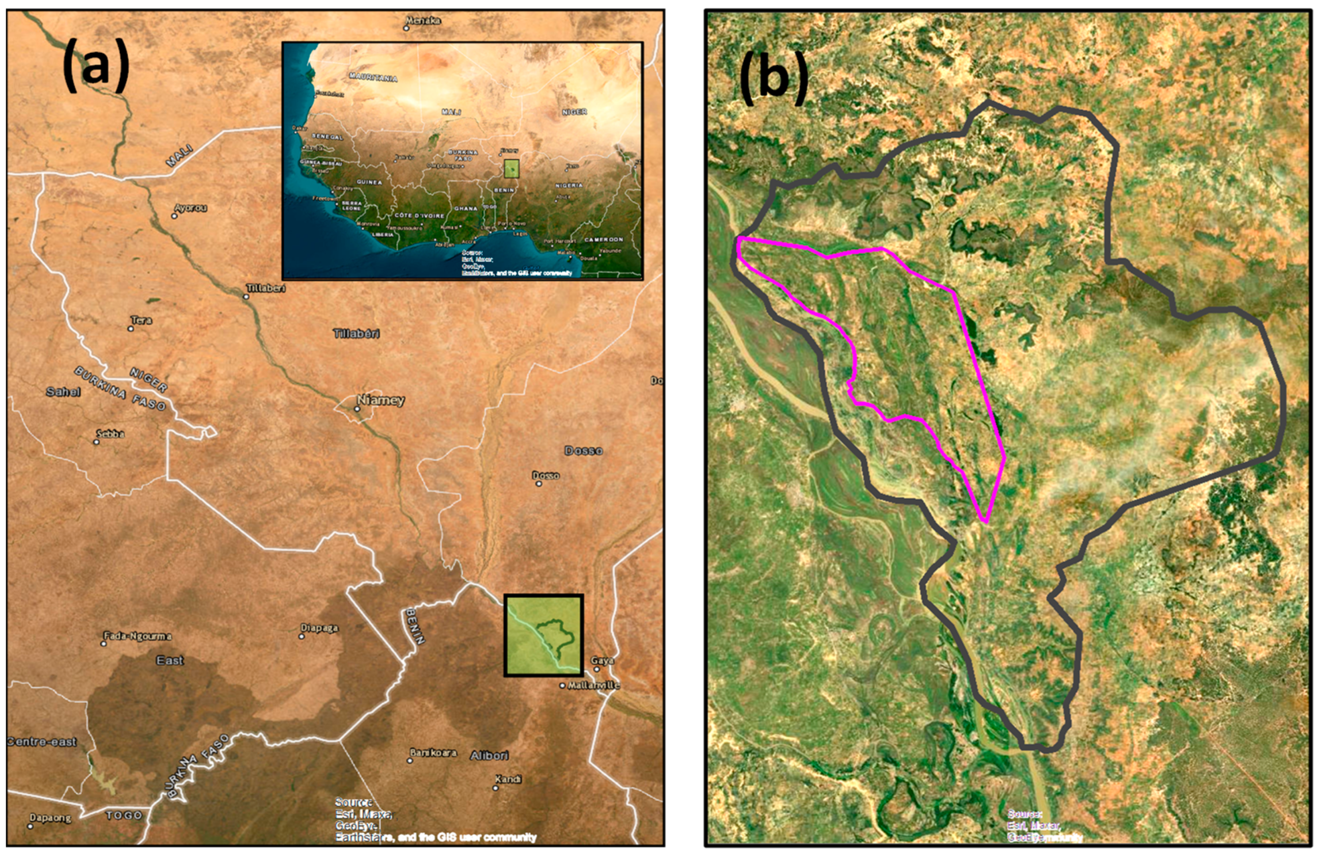
Sia Kouanza is an area in the Department of Gaya, Region of Dosso, in southwestern Niger (Figure 1a). The area of Sia Kouanza described in this study has been identified as a potential location for expanding agriculture through irrigation with groundwater. The area of primary interest for development is the “terrasse” (also called the Basse Terrasse), which is outlined in pink in Figure 1b.

Figure 1.
Maps showing: (a) the location of Sia Kouanza in the Sahel of southwestern Niger, West Africa; and (b) the outline of the model domain is in black, and the area of primary interest for development—the terrasse—is outlined in pink.
Expanding agriculture is key to promoting food security in Niger, a landlocked Sahelian country with a population growth rate of 3.7% per year [1]. Approximately 80% of the population’s livelihood relies on smallholder agriculture and livestock [2]. In the Sahel, scant and irregular rainfall results in crop deficits and, especially when compounded with drought, can lead to famine. This, in combination with conflict in neighboring countries, floods, and high food prices, can lead to food insecurity; it is estimated that 47% of children under the age of five are chronically malnourished [1]. Expanding agriculture that is irrigated with groundwater may help offset crop deficits and support food security.
Estimates on the potential of irrigable land in Niger range from 270,000 hectares (ha) from surface water alone to 10.9 million ha when irrigated by groundwater, though it depends on the depth of groundwater [3]. It is unclear what fraction of the total has been developed since the total itself has not been well-established.
Studies that describe groundwater resource development in Niger are not a new undertaking. Drought between 1965 and 1973 resulted in some of the earliest found reports, one of which noted that the majority of the available literature was located in France and had not been translated [4]. Food insecurity, famine, and malnutrition resulting from this drought spurred the creation of the United Nations International Fund for Agricultural Development (IFAD).
By the early 1980s, it was recognized that inconsistent rainfall resulted in moisture stress and agricultural yield reductions during 2 out of 10 years for crops and that groundwater resources could be developed along the Niger River, though it could require extensive technology and the resources might be fragmented [5]. A United States Agency for International Development (USAID) review of the irrigation sector commented that an economical solution to recurring drought is temporary “mining” of groundwater resources, noting insufficient data and suggesting that development be determined on a case-by-case basis [6]. The review also suggested groundwater resource monitoring be linked with proposed and underway studies. Continued and prolonged periods of inconsistent rainfall across the Sahel during the 1980s raised awareness to understand the underlying climatic causes and build resiliency.
Between 1991 and 1992, the Hydrologic Atmospheric Pilot EXperiment in the Sahel (HAPEX-Sahel) studied climate and aridification at study sites near Niamey [7]. Though groundwater was not studied as a subject in its own right, HAPEX provided information that supported groundwater studies. These studies led to a better understanding of topics including recharge infiltration processes, observations of general groundwater level increases that were attributed to drought recovery and land use change, and estimates of regional recharge [8,9,10,11].
The African Monsoon Multidisciplinary Analysis Couplage de l’Atmosphère Tropicale et du Cycle éco-Hydrologique (AMMA-CATCH) followed HAPEX Niger in the early 2000s with the addition of study sites in Benin, Mali, and Senegal to create a transect across the West African landscape [12]. Specific goals related to climate, land use, and the water cycle included global changes in the critical zone, uniting multidisciplinary researchers to detect these changes, and disseminating data and associated results outside of the academic community [13]. Continuous measurements of groundwater levels led to a better understanding of recharge distribution, rising groundwater tables due to surficial land use changes, and subsurface aquifer conditions [11,14]. It is noted that the Niger site is not listed on the AMMA-CATCH website at the time of writing.
Recent efforts to increase understanding include the use of remotely sensed data. The NASA Gravity Recovery and Climate Experiment (GRACE) satellite data have been used to evaluate changes in groundwater storage in areas of central and eastern Niger with the intention of informing water resource management [15] and supporting the long-term rise of groundwater levels in the Niger River Basin [16]. A groundwater-surface simulation for an area near Niamey basin showed ephemeral streams recharging groundwater, groundwater to be flowing primarily from the aquifer to the Niger River, and plant transpiration to dominate the water balance [17]. An effort to understand groundwater recharge/discharge dynamics and inform sustainable water resources management identified paleochannels as a source of groundwater flow to the Niger River [18].
It is likely that future efforts will increasingly employ machine learning techniques and artificial intelligence to increase understanding. For example, one study compared synthetic estimates of groundwater levels with GRACE data and limited observations in central Niger and concluded that a “storage change trend reasonably matched” [19]. Reliable synthetic estimates could be a significant contribution for areas that lack in situ measurements, not just of groundwater but other aspects of natural systems.
Despite the efforts described above and those not summarized here, Niger and greater West Africa remain data-scarce and under-represented not just for groundwater resources but science as a whole. Galle et al. [13] note difficulties in documenting environmental changes and understanding tipping points because of inadequate in situ measurements at multiple scales and uncertainty of climate simulations, especially in tropical and semi-arid areas. Measurements and simulations aside, obstacles identified for African research and its researchers include inadequate facilities and funding, limited collaborators, and underdeveloped academic writing skills, especially when English is a second language [20]. From our experiences, we note difficulties with information that is not open-access (much of the literature review above) and grey literature that must be used but is difficult to search for, use, evaluate, and justify, especially for the peer-review process. Much of the work carried out by non-governmental organizations and aid agencies resides in the grey literature.
As plans for expanding agriculture through irrigation with groundwater proceed in Sia Kouanza, we (hereafter also referred to as the team) posed several questions that could be addressed with the use of a groundwater model. The project’s questions, which ultimately became modeling objectives, included how many hectares can be developed for irrigation, where are wells most ideally located, how much water is available, and how is groundwater being replenished.
The research questions for this portion of the project are as follows: can we use existing information to develop a conceptual model and then a calibrated numerical model for a steady-state representation of a natural system where groundwater development will take place? The overarching research question is as follows: can we document changes and understand tipping points to support sustainable groundwater development for agriculture? The intent is to provide an open-access framework that can be employed in data-scarce areas where similar questions are being asked. Developing sustainable groundwater for agriculture reaches scales beyond Sia Kouanza to the world’s estimated 2.5 billion smallholder farmers, whose livelihoods could be improved, and children who could be fed [21].
The goal of this article is to describe an approach to groundwater modeling, beginning with data collection through a conceptual model and moving to a steady-state calibrated numerical model. A steady-state model is a necessary starting point for transient and predictive models that can address overarching project questions. It is noted that a steady-state model is intended to represent “average” annual conditions in the groundwater system prior to changes, in this case, groundwater development for agriculture. Approaches for transient and predictive models, which can be used to simulate changes in irrigation pumping volumes and drought, for Sia Kouanza will be described in subsequent publications.
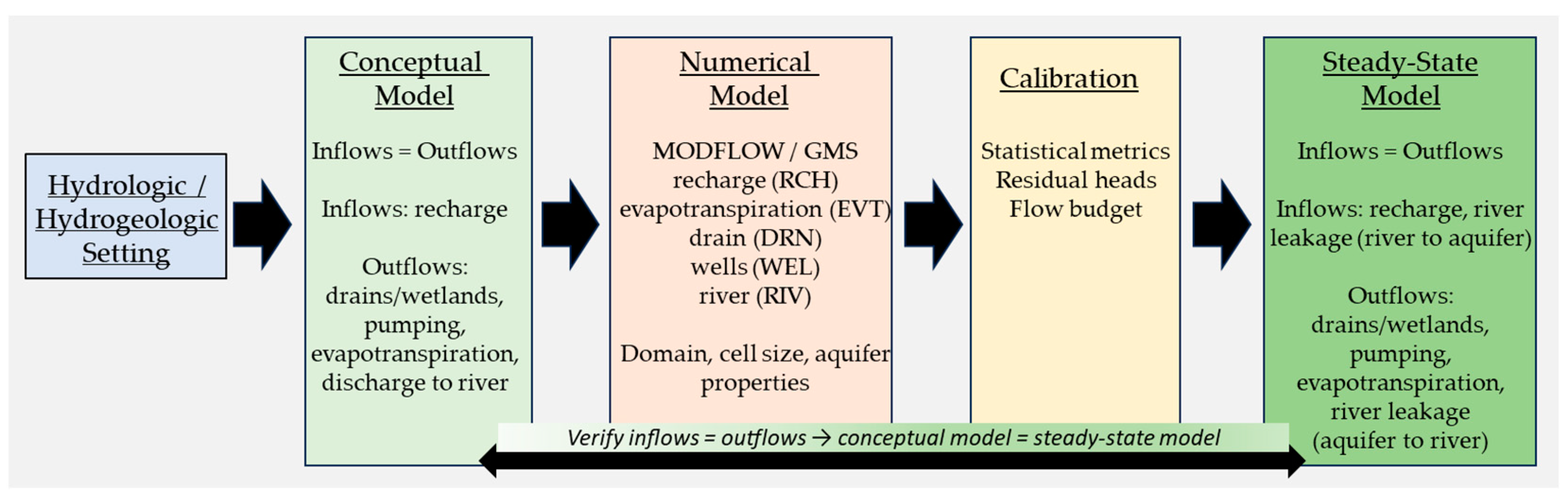
Numerical models are useful tools for evaluating groundwater availability and sustainable use, understanding hydrogeological processes, assessing potential environmental impacts, and long-term planning [22]. While there is abundant literature describing their utility, it can be difficult to find procedures and details for model construction, especially when data are scarce. The approach employed here describes the hydrologic and hydrogeologic setting, development of a conceptual model, understanding the water balance, choice of numerical code, construction of a numerical model, calibration of that model, and interpretation of the calibrated steady-state model (Figure 2).
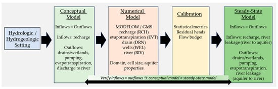
Figure 2.
Diagram of the approach employed for the Sia Kouanza model, describing the setting, conceptual model, numerical model, calibration, and steady-state model.
2. Materials and Methods
The following section describes materials and methods for the approach to groundwater modeling, beginning with data collection through a conceptual model and ending with the construction of a steady-state model.
2.1. Hydrologic and Hydrogeologic Setting
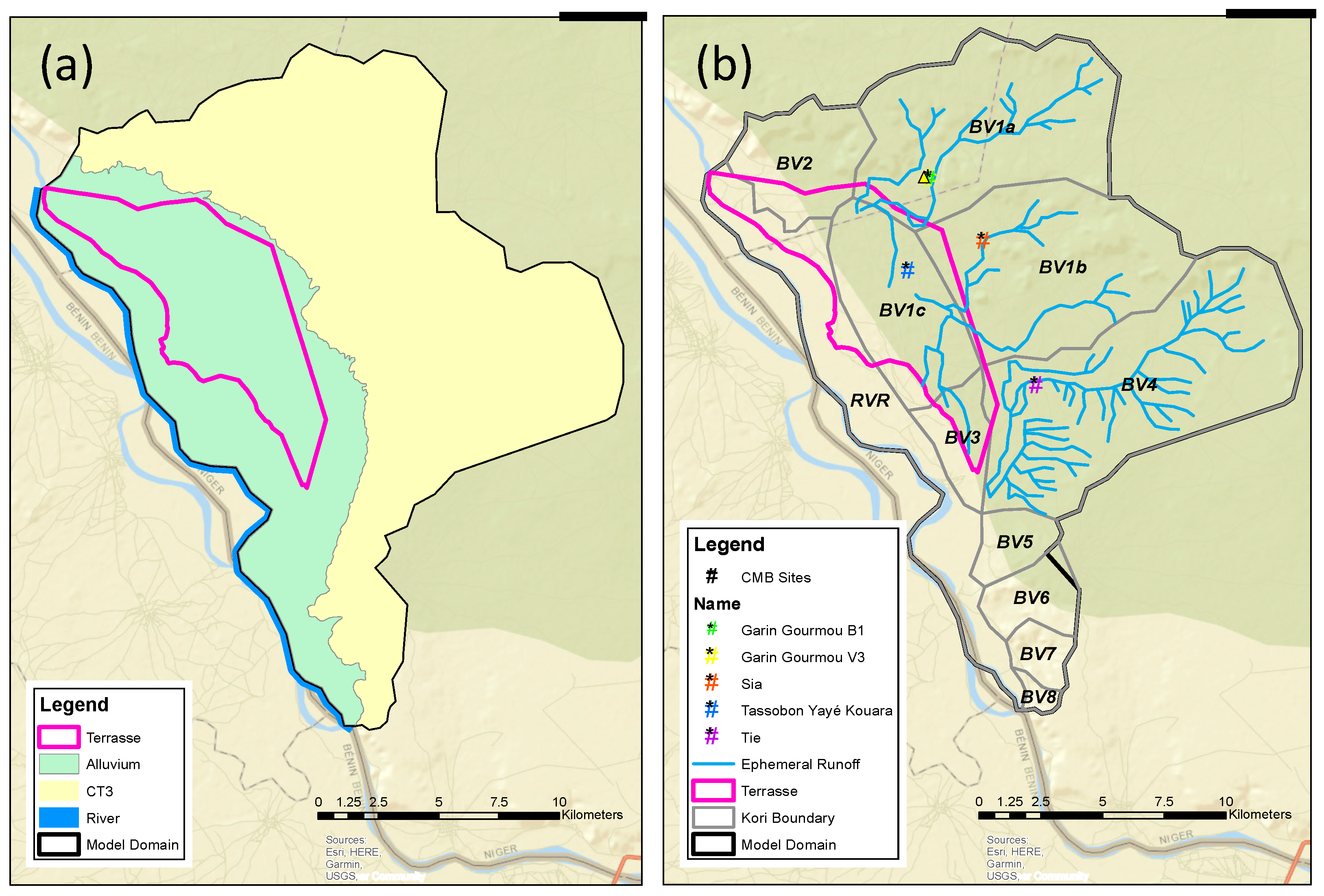
The Sia Kouanza area is bounded along the western side by the Niger River, which flows approximately 30 km from the northwest to the southeast (Figure 3a). At its widest, the Sia Kouanza area is approximately 28 km by 20 km north to south and west to east, respectively. The terrasse is outlined in pink. The terrasse is approximately 15 km from northwest to southeast and 5.5 km from southwest to northeast.

Figure 3.
Maps showing: (a) the location of the Sia Kounza modeling domain in black, the terrasse area of primary interest outlined in pink, and hydrogeologic setting of the domain in yellow and green; and (b) delineation of kori watersheds outlined in black and denoted as BV1 through BV8, ephemeral surface water runoff as blue lines, and chloride mass balance (CMB) sample sites shown as triangles.
The terrasse consists of an anastomosing network of paleochannels of the Niger River. It is unclear when the river last inundated the terrasse, but it currently is not in the active flood plain. On satellite imagery, the paleochannels appear visibly greener due to relatively higher soil moisture content in lower topographic settings (Figure 1b). In these settings, paleochannels predominantly consist of coarse-grained deposits of sands and gravels that are in contact with finer-grained deposits of bedded clays, silts, and fine sands. The coarse deposits convey groundwater closer to the land surface, identified as a groundwater discharge [18], and support greener vegetation. The combination of coarse and fine deposits produces a discontinuous mosaic in the terrasse—a large range of particle sizes at depth over short distances, which is reported in driller’s borehole logs.
The uppermost geological formation in this area is primarily composed of alluvial materials, which transition to the sandstone of the Continental terminal (Ct3) aquifer to the northeast. Underlying both the alluvial materials and the Ct3 formation are the clayey Continental intercalaire (Ci) and Continental hamadien (Ch) aquifers (Figure 3a). These aquifers are difficult to distinguish and considered undifferentiated in this area and are hereafter referred to as the Ch/Ci aquifer. This Ch/Ci aquifer thins in the direction of the Niger River, creating a wedge shape. Bedrock underlies the Ch/Ci formation and is exposed at the surface across the Niger River to the southwest. An extensive investigation of the spatial distribution and thickness of the Ct3 and Ch/Ci aquifers can be found elsewhere [23].
The extreme northeastern portion of the study area hosts several sandstone plateaus. Land surface elevations slope downwards towards the Niger River from northeast to southwest. Runoff in these upgradient watersheds flows through koris and is delivered to downgradient areas (Figure 3b). A kori is a local term for a shallow valley that carries ephemeral runoff and can be thought of as being similar to a “wash” of the Western United States. In the downgradient areas of the terrasse, a portion of runoff is captured in small dams or diverted through channels for use in agricultural irrigation, while the remainder makes its way to the Niger River.
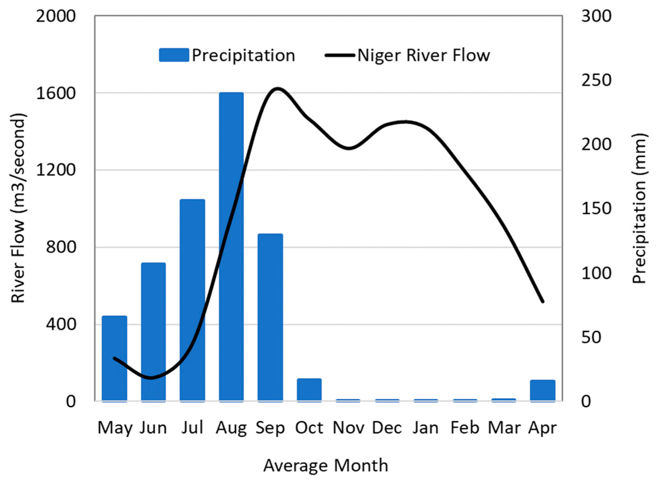
Annual precipitation in the Sia Kouanza area varies between 600 and 800 mm [24] and generally falls during the “wet” or “rainy” season months of May through October (Figure 4). The remaining months are the dry season. The figure shows average monthly precipitation from a gridded dataset (CHIRPS, explained below) representing the area between 1981 and 2021. More detailed information on local precipitation is provided in the conceptual model, Section 2.2.

Figure 4.
Average monthly Niger River flow (between 1952 and 2021) and precipitation (between 1981 and 2021) in the Sia Kouanza area. Seasonal variability is observed for both precipitation and river flow.
Surface water resources in the area are dominated by precipitation and the Niger River. Figure 4 shows average monthly river flow measured at the Malanville gauge, which is approximately 40 km downstream of the study area, between 1952 and 2021. Seasonal variability is observed—a rapid rise in stage with the onset of precipitation followed by a gradual decline into the dry season. A second smaller and rounded peak is noticeable during December and November, which is anecdotally attributed to the delayed emptying of the Niger Inland Delta upstream in Mali.
2.2. Conceptual Model
The importance of developing a conceptual model prior to embarking on a numerical model should not be underestimated, as it is one of the most important steps for any model [25]. Definitions of a conceptual model vary from “the hydrologist’s concept of a ground-water system” [26] to more detailed descriptions of hydrogeological units and boundaries [27]. In Sia Kouanza, the conceptual model needed to support model objectives to address the questions posed by the team.
In order to address questions about groundwater development and use, a conceptual model of water balance is needed to support a steady-state model. The water balance provides a preliminary flow budget. This budget is then needed for numerical model calibration. The flow budget generated by the numerical model should be comparable to the conceptual model flow budget.
Sia Kouanza has no known water balance, so this was a starting point. The principal components of the Sia Kouanza conceptual groundwater model are recharge from precipitation, groundwater flow to and from the Niger River, groundwater evapotranspiration, groundwater discharge to ponded surface water in the terrasse (wetlands and drains), and extraction at existing community wells. For the purposes of a steady-state model, all components represent “average” annual conditions. The components are described separately below.
2.2.1. Recharge from Precipitation
Recharge occurs from infiltration of precipitation during the wet season months. Precipitation data are recorded locally at four locations in and around the modeling area—Ecole Centre Tanda, Tanda Radio Bassiyena, Rountoua Malam Kouara, and Tanda Mairie. Data were not available for these stations prior to 2015, so Climate Hazards Group InfraRed Precipitation with Station (CHIRPS) data were considered to calculate a long-term average [24]. CHIRPS captures remotely-sensed tropical precipitation over a larger area and longer time, so it is useful as a means of comparison and infilling when measured data are not available.
Measured monthly precipitation amounts from the four locations were compared with monthly CHIRPS data for corresponding months during years 2015 to 2021 (Figure 5). Pearson’s r was employed to evaluate the strength of the linear relationship between monthly measurements of local stations and CHIRPS. Data that plot one-to-one along a straight line with a positive slope are positively correlated (Pearson’s r = 1), while data that plot one-to-one along a straight line with a negative slope are inversely correlated or −1. Values closer to ±1 have a stronger relationship, while values closer to 0 have no strength of relationship. More detail on Pearson’s r can be found in Helsel et al. [28].
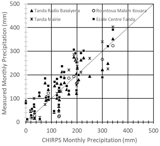
Figure 5.
One-to-one plot of monthly CHIRPS precipitation and measured monthly precipitation between 2015 and 2021.
The Pearson’s correlation coefficients indicated a strong positive relationship between CHIRPS and each of the four locations (Ecole Centre Tanda = 0.84; Tanda Radio Bassiyena = 0.84, Rountoua Malam Kouara = 0.86, Tanda Mairie = 0.90). Thus, CHIRPS data could be used when no local data were available for the study area. The CHIRPS average annual precipitation between 1982 and 2020 is 732 mm per year; this value was used to estimate recharge for the model.
Only a portion of precipitation enters the groundwater system as recharge. Different approaches are used to estimate recharge. For this study, we used a chloride mass balance (CMB). The CMB has been used to estimate groundwater recharge in semi-arid areas around the world [29,30,31].
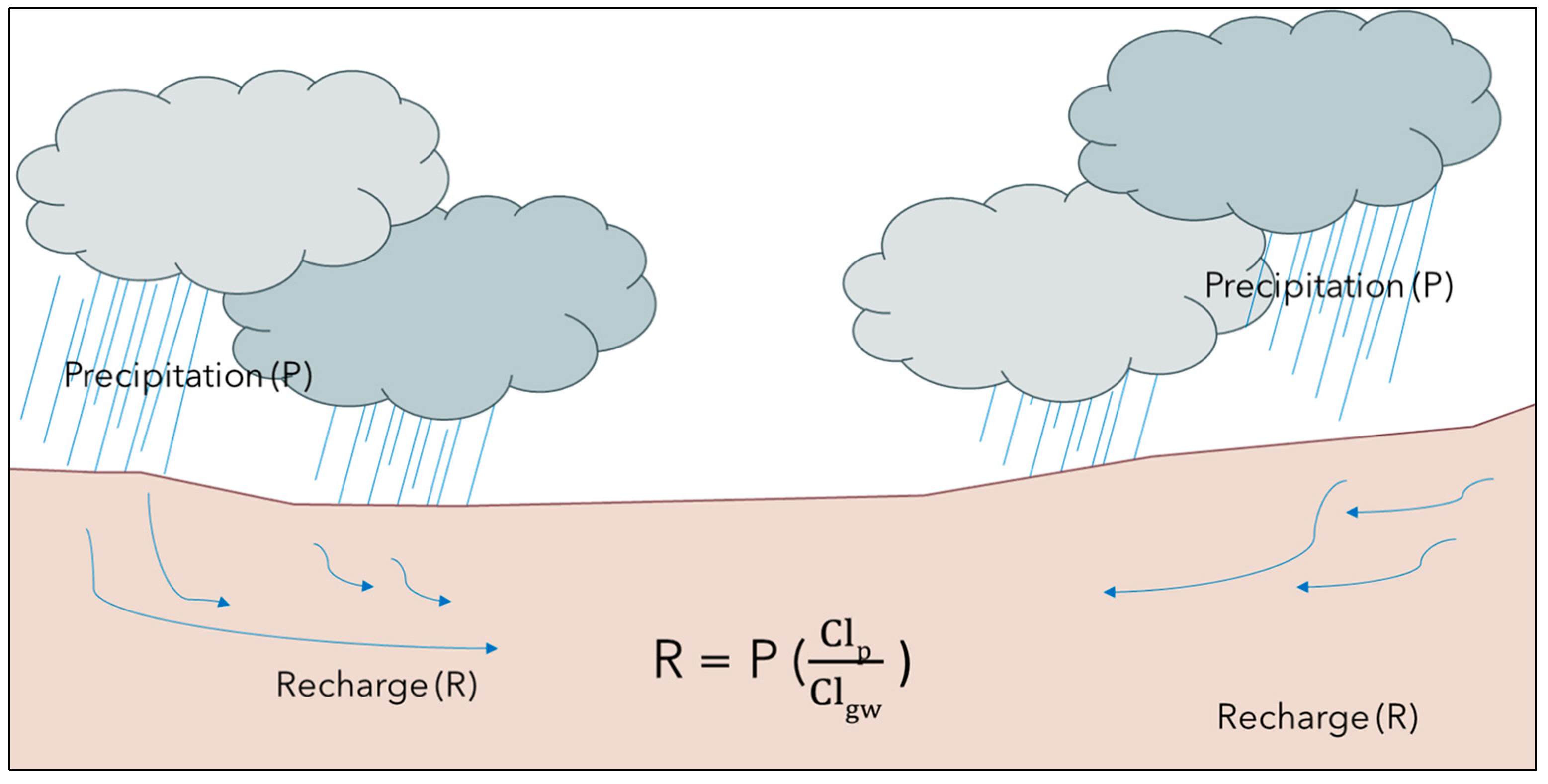
The simplicity of the CMB makes it ideal for remote areas since it only requires measurements of annual precipitation, chloride concentration in the precipitation, and chloride concentration of groundwater. It is inexpensive, needs no instrumentation, does not require sampling during an event, and is independent as to recharge being focused or diffuse. The technique is based on chloride being a conservative environmental tracer that is neither gained nor lost from a groundwater system due to adsorption or desorption processes. Chloride originates from precipitation and is transported by water infiltrating the subsurface (Figure 6). The CMB can be used to estimate groundwater recharge over a range of temporal and spatial scales.
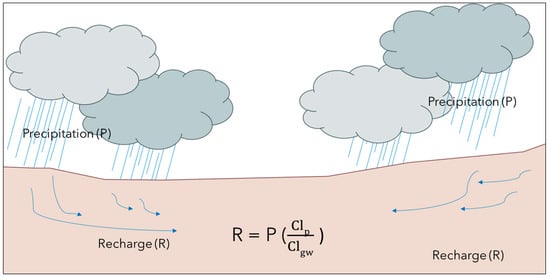
Figure 6.
Sketch of the chloride mass balance (CMB) approach. Chloride originates from precipitation (P) and is transported to groundwater by water infiltrating the subsurface (blue arrows) as recharge (R).
Some assumptions of the CMB include that chloride is not stored in the soil, precipitation is the only source of chloride in groundwater, and chloride is conservative in the system and does not react [31]. When these assumptions are met, recharge (R) can be estimated by calculating a ratio of the chloride measurements in precipitation and groundwater:
where
- P is the average annual rainfall (m);
- Clp is the average Cl concentration in precipitation (mg/L);
- Clgw is the average Cl concentration in groundwater (mg/L).
There is a paucity of measurements of chloride in precipitation for this area of West Africa. Samples collected in 1992 during the HAPEX project in Niamey ranged in value from 0.29 to 0.51 mg/L, with the range attributed to the trajectory of storms as they move inland from the coast [32]. More recent measurements of chloride in precipitation were taken from a CMB recharge study in northern Ghana [33]. Sia Kouanza is located along a climatic gradient approximately between Niamey and northern Ghana. The value of 0.40 mg/L chloride in precipitation measured by Krautstrunk [33] compares with 0.39 mg/L, which was observed in another recent recharge study in northern Ghana [34] and falls in the middle of the range of values observed along the HAPEX transect. The relative consistency of chloride in precipitation across time and space supports use of the value.
Measurements of chloride in groundwater were taken from samples collected by the team in the study area. A subset of samples was used for calculation of recharge. Samples were not used when driller’s logs reported presence of clays at sites, which can impede recharge, and when measurements were two standard deviations above the average chloride measurement. In general, sites located closer to the koris were prioritized over sites in the terrasse, as sites in the terrasse may experience pooling and effects from the river.
Applying these criteria resulted in the use of the subset of five sites that were used for the CMB: Garin Gourmou-1, Garin Gourmou-2, Sia, Tassobon Yaye Koira, and Tie (Figure 3b). The range of chloride values is shown in Table 1. The table shows the calculation of an average recharge of 0.09 m or 12% of precipitation. The CMB gave an estimation that served as a guideline for further refining recharge rates across the study area.

Table 1.
Calculation of recharge at sites using the chloride mass balance (CMB).
Recharge rates are not typically homogenous across an area. Values likely vary between the watersheds of the terrasse and koris and among all the koris. A simulation developed on the US Army Corps of Engineers Hydrologic Engineering Center’s (HEC) River Analysis System [35] was created as part of a separate study to understand movement of surface water into the terrasse and Niger River from the koris. A summary of the HEC simulation is given below, and more details are described in another report [36].
The HEC simulation used daily rainfall and evaporation data beginning in 1960 from a weather station at Gaya for daily timesteps between 1981 and 2015. A 0.5 m resolution LIDAR survey was conducted for topography of the terrasse and an area westward to the Niger River bank at a low water level during May 2016. Kori runoff coefficients are based on Soil Conservation Service values for loamy sandy soil, silty sandy soil, and sandy dune soil [37,38] and land uses of savanna culture mosaic as well as shrub savannah and hill vegetation.
Runoff coefficients are dimensionless and describe the proportion of runoff or infiltration formed from precipitation. Values closer to 1 indicate higher runoff and lower infiltration, such as steep or paved areas, while values closer to 0 indicate lower runoff and higher infiltration, such as vegetated areas [16]. Statistical metrics were not reported for the HEC simulation, though one-to-one plots showed even distribution with no high or low bias of simulated and observed data.
The koris are not instrumented for precipitation or runoff, and local recharge data are not available, so the HEC simulation served as a point of departure for estimating recharge. The year 2017 was simulated because it most closely approximated an average year of 732 mm of precipitation. Recharge coefficients for each kori are listed in Table 2. The kori watersheds shown in Figure 3b are the same as those used in the HEC simulation.
Table 2.
Recharge coefficients and final recharge rate for each kori.
A comparison of the estimated total recharge for the model domain using the CMB and the HEC simulation showed the former to be 61% of latter. The HEC simulation recharge rates for each kori were multiplied by the land surface area and 0.61 to scale recharge from HEC to CMB. Thus, each kori maintained its variability of recharge rate, which was defined by the HEC simulation. Further scaling was performed to some of the “downstream” koris to account for pooling. Using this method, total average recharge was estimated to be approximately 22 × 106 m3/year.
2.2.2. Evapotranspiration
Besides leaving as outflows to the Niger River, groundwater in the study area also outflows as evapotranspiration (ET) via phreatophytes (deep-rooted plants that use groundwater) and riparian plants. Estimating ET is a challenge. For example, advection can undermine the utility of ET estimates from gridded climate products representing semi-arid environments with irrigated, dryland, and native vegetation land cover [39]. Even in extremely intensively instrumented and studied areas, such as the Colorado River basin, there are ongoing debates and implied major uncertainties in estimates [40]. Further work and potentially a site visit are required to better understand local ET. Until that is possible, we accept this is an area of uncertainty in our study.
The team used an approach based on values of phreatophyte ET and climate similarities between southern Nevada and Sia Kouanza. Pahrump Valley in southern Nevada is semi-arid, characterized by annual precipitation just under 1000 mm that occurs during several months of the year (winter monsoon), evaporation rates up to 2500 mm/year, and ephemeral runoff that flows through washes (koris), where some are captured in small dams or diverted through channels for use in agricultural irrigation [41]. For reference, the HEC model described above used an annual average ET value of 2190 mm.
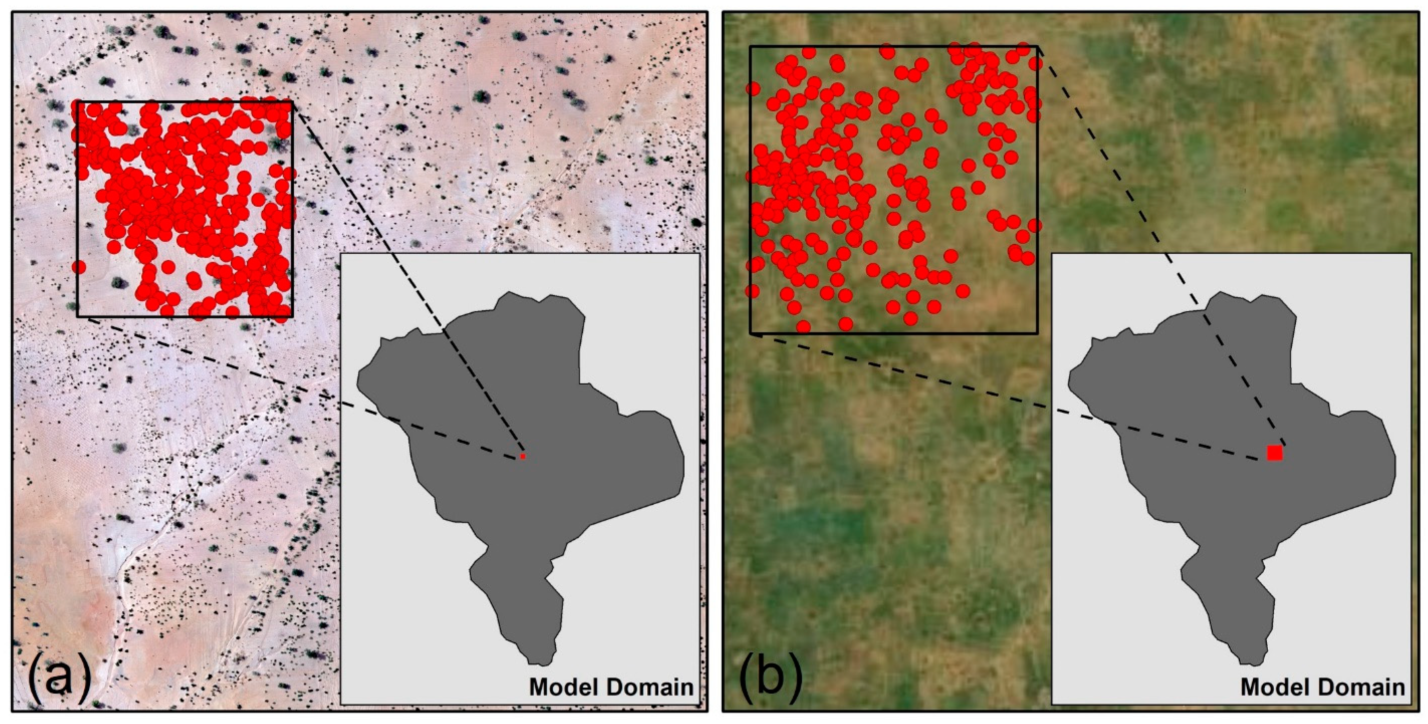
Phreatophyte ET for Sia Kouanza was estimated by making a spatial count of shrubs and trees in two randomly selected squares in the BV1b kori watershed (Figure 7). Shrubs were identified within a 250 m × 250 m square of a high-resolution Lidar flight imagery collected over the terrasse area for use in this study (Figure 7a). Trees were identified from Landsat imagery within a 1 km × 1 km square (Figure 7b). A water use rate of 1 m/yr was assumed using the estimated ET rate of mesquite in the Pahrump Valley proxy site [41].
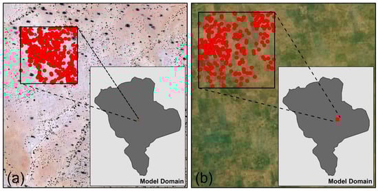
Figure 7.
Identification of vegetation from satellite imagery. (a) Smaller shrubs were identified from the higher resolution Lidar flight imagery collected over the terrasse area for use in this study, within a 250 m × 250 m square. (b) Trees were identified from Landsat imagery within a 1 km × 1 km square.
Table 3 shows values for the average ET rates of trees and shrubs. Assuming that the observed density of the mesquite plants is representative of the model domain, the average annual ET rate in m/d was multiplied by the area of the model domain, excluding the riparian watershed, for a total estimated phreatophyte ET rate of 8.3 × 10⁶ m3/year.
Table 3.
Summary statistics for estimated average annual evapotranspiration (ET).
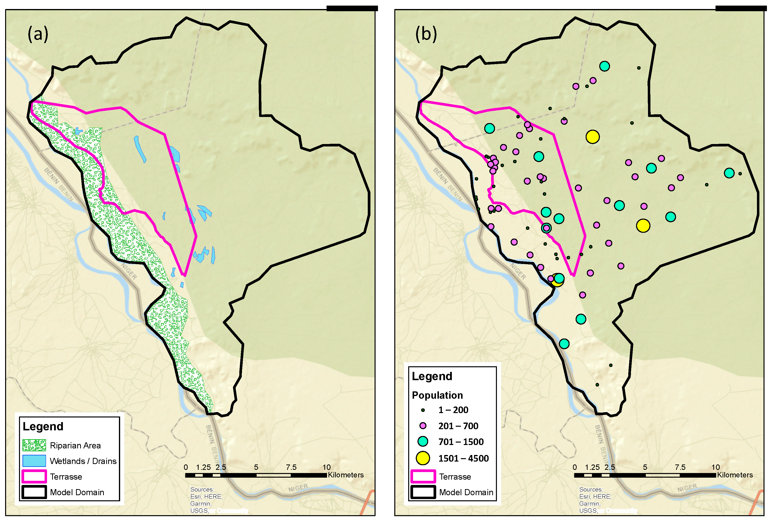
Riparian ET was estimated separately for an area directly along the river (Figure 8a). Review of satellite imagery shows this area to generally appear greener and support greenness longer as compared with elsewhere in the modeling area. An inventory of plants in the riparian area was not available, so some conservative assumptions were made. ET rates were estimated using a value representative of rice, a crop that has a relatively high water consumption as compared with other crops (0.864 m per crop) and is flooded periodically, on a regular basis, similarly to riparian vegetation in monsoonal areas [42]. It was assumed that one-third of the land is covered by one rice crop that uses groundwater for four months of the year. The remaining two-thirds of the land may be flooded by river water or surface runoff or be fallow. It was assumed that rice uses groundwater during the driest part of the year. The estimated volumetric ET rate in this zone is 3.6 × 10⁶ m3/year.
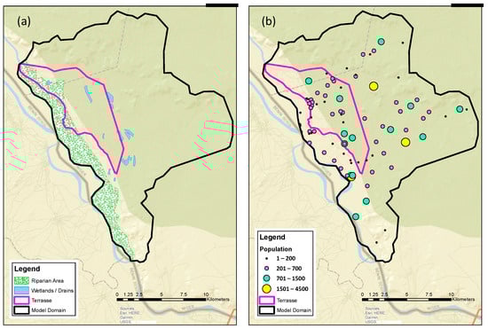
Figure 8.
Maps showing: (a) the delineation of riparian areas (green) along the southwest boundary, which is also the river and locations of wetlands (blue) in and near the terrasse (pink) believed to be fed by groundwater; and (b) locations and populations of existing communities shown in the terrasse (outlined in pink) and larger modeling domain (outlined in black).
2.2.3. Wetlands/Drains
Several wetlands—believed to be fed by groundwater discharging to the surface—exist in the terrasse (Figure 8a). Wetlands are also referred to as drains in this study for the MODFLOW package used to represent them. No measurements of flow or evaporation are known to exist for these wetlands, so a proxy site was used to make estimates [43]. Lake Hodges in Southern California, USA, experiences a climate similar to that of the study area. The area surrounding Lake Hodges is semi-arid, characterized by annual precipitation up to 800 mm that occurs during a few months of the year (winter monsoon) and annual ET near 2000 mm. Surface water evaporation at Lake Hodges was measured during a multi-year study; these values were used for wetland evaporation in Sia Kouanza.
Based on the Hodges information, surface evaporation rates for the drains at the study site were estimated at about 736 mm/year. This value multiplied over the surface area of the wetlands gives an estimated evaporation rate of 2.1 × 10⁶ m3/year for the wetlands.
2.2.4. Extraction from Existing Wells
Groundwater extraction in the Sia Kouanza area currently takes place at community wells that are either hand-dug or drilled boreholes (Figure 8b). To estimate extraction rates at these wells, we considered that each community member in the Sia Kouanza area should have access to 50 L per capita per day (lpcpd) from these wells.
This number falls within a World Health Organization (WHO) guideline [44]. The WHO indicates 20 lpcpd to be basic access for domestic water use, which includes drinking, cooking, and hygiene. This amount is to be a guideline in communities where a well is located between 100 m and 1 km, 5 to 30 min are spent collecting water, and bathing as well as laundry take place at the well. Fifty lpcpd is intermediate access for domestic use, in communities where a well is located within 100 m or water is delivered into the household through a tap, five minutes is spent collecting water, and bathing as well as laundry take place in the household. Intermediate access scenarios allow water for gardening.
Most community members in the Sia Kouanza area are likely to have basic access to 20 lpcpd. Very few households, if any, have a tap delivering water. Smaller communities often access a more distant well that is shared with another community or several communities. Using the intermediate access higher value of 50 lpcpd as a conservative assumption ensures each community member at least basic access as well as some additional water for increased demand due to economic growth and population. Total community extraction rates were calculated by multiplying population by 50 lpcpd. The total estimated extraction from existing community wells is 7.2 × 10⁵ m3/year.
2.2.5. River
The Niger River forms the southwestern boundary of the model. There are no gauges for either stage or volume in the study area, so river stage was obtained from the HEC model, which created transects along the river. River stage was simulated for the year 2020 because it is the first year during which time-series groundwater levels were measured, and a comparison of groundwater levels with river stage is necessary. It is difficult to estimate the amount of groundwater discharging from the aquifer to the river; further work involving stream gaging would benefit the study. Until that is possible, we accept this is an area of uncertainty. Based on other components of the flow budget, the amount was estimated to be 7.3 × 10⁶ m3/year.
2.3. Conceptual Model Preliminary Flow Budget
The preliminary flow budget describing the inflows and outflows of the conceptual model is shown in Table 4. Recharge, river discharge, ET, and extraction rates were derived as described in the previous sections. Phreatophyte ET and riparian ET are grouped in a lump sum, calculated as total ET (8.3 × 10⁶ + 3.6 × 106 = 11.9 × 10⁶ m3/year). Once finalized, the preliminary flow budget and measured groundwater elevations will be used to calibrate the groundwater model.
Table 4.
Conceptual model flow budget.
2.4. Numerical Model
The software MODFLOW-NWT (version 1.3.0) [45] was used to simulate the three-dimensional groundwater flow system in the basin. MODFLOW is considered the industry standard and has been extensively tested and verified by numerous hydrogeologists. The model was developed within the Groundwater Modeling System (GMS) environment (version 10.7). GMS facilitates pre- and post-processing of hydrogeologic information for MODFLOW and provides a graphical interface.
The principle of parsimony was applied to develop the Sia Kouanza model. The principle calls for keeping the model as simple as possible while accounting for the system processes and characteristics that are evident in the observation and are important to the prediction and while respecting all system information [46]. A steady-state model representing pre-development conditions was calibrated to match observed groundwater levels (head) to simulated head while also fitting MODFLOW-generated flow budget values to the conceptual model preliminary flow budget. The results of this model were used as the initial condition for a transient model simulating the years 2024 through 2034, using monthly stress periods.
The following MODFLOW packages were used: recharge (RCH), evapotranspiration (EVT), drain (DRN), wells (WEL), and river (RIV). The RCH package requires recharge values as a flux distributed aerially over the top of the model (polygons) in units of m/day. Estimates of recharge as coefficients (a fractional value) for each kori watershed are given above.
The EVT package requires maximum evapotranspiration as a flux distributed aerially over the top of the model (polygons) in units of m/day. Also required is an extinction depth, which simulates evapotranspiration as a function of depth to water from a specified surface—in this case, the land surface. Evapotranspiration rates are calculated as a linear function where the maximum evapotranspiration rate is applied at the surface and decreased linearly until the extinction depth is reached. Thus, simulated evapotranspiration is higher in areas with shallow groundwater and lower in areas with deeper groundwater. For this model, the extinction depth is 20 m in the koris and 2 m along the river. Maximum ET rates are based on the mesquite in the Nevada proxy site [41] for the koris and rice along the river, as described above.
The DRN package requires a bottom elevation and a conductance term for each drain. Simulated drains are a head-dependent flux boundary, as groundwater is only allowed to discharge at a drain where the simulated groundwater elevation is greater than the assigned bottom elevation at that drain. The discharge rate is a function of the difference between the groundwater elevation and the drain bottom elevation. It is scaled by the conductance term, which describes the sediment at the base of the drain. Simulated drain bottom elevations were set according to observed land surface elevations at the locations of the wetlands, and conductance terms were calibrated to estimate groundwater discharge to the wetlands while also maintaining a good fit with observed water levels. All drains were assigned a conductance of 0.1 (m2/d)/m2.
The RIV package requires head-stage (stage) elevation and bottom elevation, as well as riverbed conductance. The stage is the level of the river surface, and bottom elevation was estimated as 3 m below the stage. Riverbed conductance is defined as the hydraulic conductivity of the material that constitutes the riverbed divided by the vertical thickness of the material of the riverbed multiplied by the surface area of the river (the length times the width). Conductance was calibrated to 50 (m2/d)/m2. The stage was defined at three points along the upper, middle, and lower sections of the river within the model domain. Steady-state stage values in the study area range from 158 m above sea level (masl) to 160 masl based on HEC model simulated values for the month of March. Stage values from the month of March were selected because they most closely represented average annual conditions.
2.4.1. Domain—Boundary Conditions
Groundwater in the study area generally flows from the northeast to the southwest, discharging to the Niger River. The kori watershed boundaries were taken from earlier reports. The Niger River formed the western boundary of the model.
2.4.2. Cell Size
Cell size in the numerical model is discretized into cells of 100 m by 100 m. There are two layers in the model. The top of Layer 1 is the land surface. The land surface is a digital elevation map (DEM) derived from Shuttle Radar Topography Mission (SRTM) downloaded from the U.S. Geological Survey Earth Explore [47]. The DEM has 90 m resolution, which was converted to the 100 m grid. The land surface varies from 156 masl along the Niger River, gradually increasing to 269 masl at the top of the escarpments in the northern and eastern portions of the model.
The bottom of layer 1 is the same elevation as the top of layer 2. It is approximately 100 m below the land surface. The bottom of layer 2 is approximately −22 masl along the river and decreases to approximately −385 masl in the eastern portions of the model due to the wedge shape of the geologic features. This elevation was determined from the investigation of the spatial distribution and thickness of the CT3 and CH/Ci aquifers mentioned above [23]. The first layer consists of both CT3 in the east of the model domain and alluvium in the west, as shown in Figure 3a. Layer 2 represents the CH/Ci.
2.4.3. Aquifer Properties
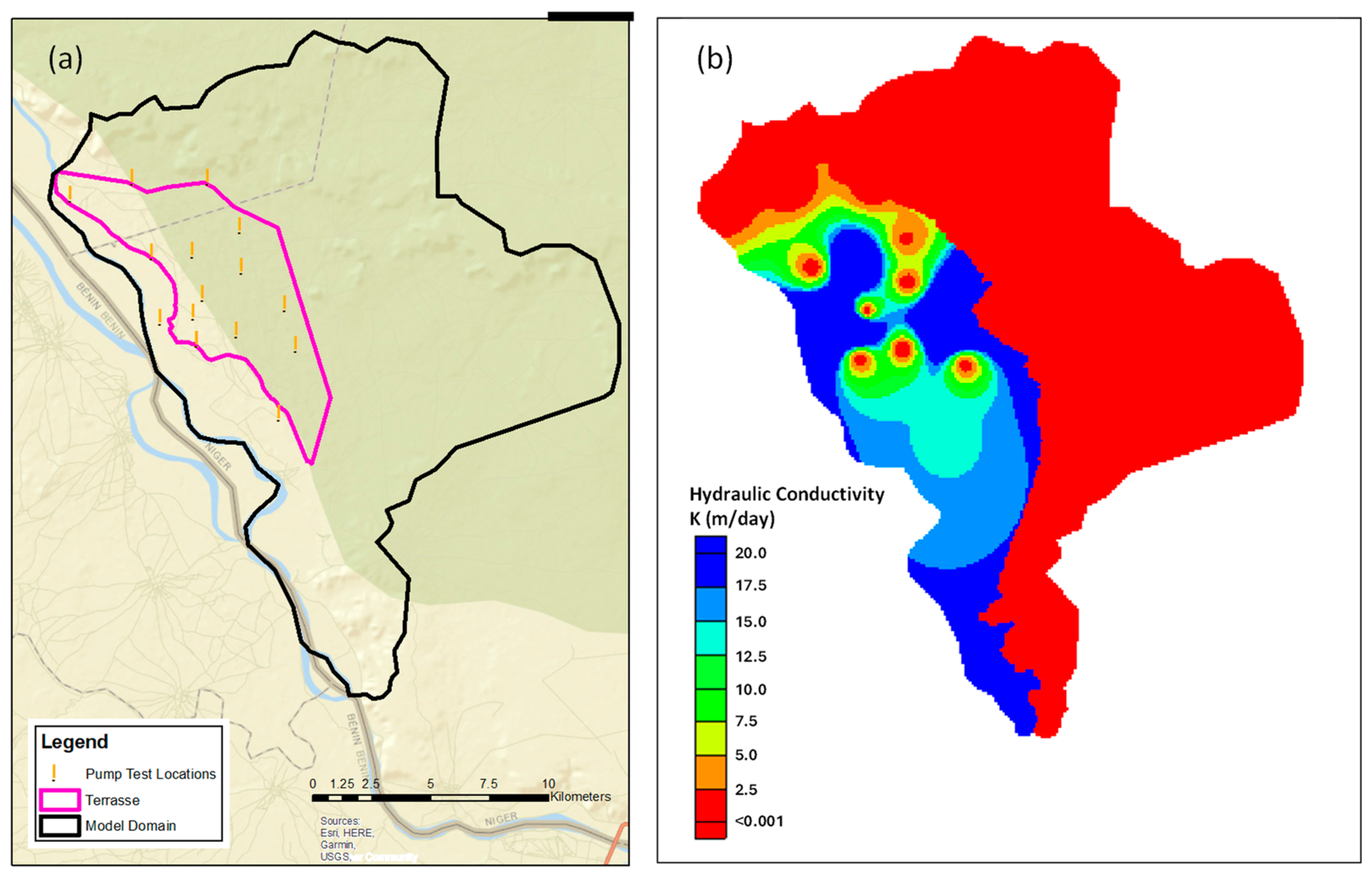
Aquifer tests were conducted in a subset of boreholes across the study area during June and July 2022 at locations shown in Figure 9a. For those boreholes where adequate data could be collected, measured water levels and pumping rates during step drawdown and constant rate tests were entered in the Aqtesolv software program (version 4.5) [48], which employs curve-fitting to estimate parameters such as transmissivity (T). The Aqtesolv program allows users to try multiple solutions to find the best fit for analysis, such as Theis, Cooper–Jacob, Moench, etc.
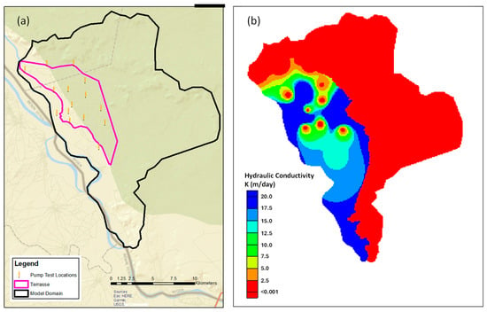
Figure 9.
Maps showing: (a) location of aquifer pump test locations in and adjacent to the terrasse (pink) that were used for pilot points of hydraulic conductivity (K); and (b) Distribution of K values based on pilot points of the aquifer pump test locations for alluvium in Layer 1 of the groundwater flow model.
Summary data are given in Table 5. Results of the curve-fitting analyses were employed as pilot points for hydraulic conductivity (K), which is calculated as T divided by the aquifer thickness. The range of K values can be explained by the presence of alternating paleochannels consisting of coarse materials and sedimentary materials such as clay. The wide range of K values can be explained by the paleochannels in the terrasse, which are a discontinuous mosaic of coarse- and fine-grained materials ranging from gravels to clays, respectively.
Table 5.
Summary of results from curve-fitting in the Aqtesolv program.
Extraction at community wells was simulated using MODFLOW’s Well (WEL) package. The well package can accept the elevation of the screened interval for each well as input, which is used to determine the model layers from which water will be extracted. Depths and screened intervals of existing community wells were unknown, and all were assumed to be screened into layer 1 only.
2.5. Model Calibration
Calibration of the steady-state model sought to match observed groundwater levels (head) to simulated head while also fitting model-generated flow budget values to the conceptual model preliminary flow budget. This process is carried out by trial and error, both manually and automatically, while employing the Parameter Estimation (PEST) package [49]. Layer 1 was simulated as being unconfined. Aquifer parameters were iterated between the two simulations to calibrate to observed trends in water levels.
Information from pump tests conducted during June and July 2022 was used to refine K in Layer 1, allowing the layer to be separated into two zones—alluvium and koris. In the alluvium, hydraulic conductivity data derived from the aquifer tests were used as pilot point interpolations as opposed to a zonal approach. Pilot points allow for individual K values to be applied at specific locations, with values interpolated in between the locations. During calibration, values of K applied as pilot point parameters were allowed to vary by ±20% from the pump tests to more correctly capture groundwater levels. Figure 9b shows alluvium K values varying between 0.001 and 20.0, with one point as high as 97.8 m/day (>20). The koris are shown as single-value zones. Three pilot points were added to constrain contours in locations where hydrologic information was scarce. The K values at these points were calibrated and were held within the range of observed values.
3. Results and Discussion
Three checks were used to evaluate the calibration of the Sia Kouanza steady-state model: statistical metrics, residual heads, and a flow budget (water balance).
3.1. Statistical Metrics
Statistical metrics employed: mean error (ME), mean absolute error (MAE), and root mean squared error (RMSE). Information on statistical metrics is available from multiple sources [28,49,50]. The goal was to minimize the values of ME and RMSE metrics and for the MAE to be less than 5% of the difference between the highest and lowest observed head. A difference of less than 5% is ideal, though the team agreed that an acceptable difference for this model would be up to 10% given that some data were scant and/or analogs were used. A summary of statistical metrics for the steady-state model is shown in Table 6. Explanations are provided below.
Table 6.
Summary values of statistical metrics used to evaluate calibration.
3.2. Residual Heads
Figure 10a shows residual heads. A residual head is the observed groundwater level subtracted from the simulated groundwater level, so it is another term to describe the error. The residual heads show the direction (positive or negative) and magnitude of the difference between the observed and simulated points. A positive residual means the simulated head is too high, and a negative residual means the simulated head is too low. The size of the circle indicates the magnitude; the small white circles show most residuals to be less than ± 1 m. The purpose of a residual head map is to observe the spatial distribution of an error and determine whether there is a bias in a specific area. The figure shows some of the larger residual heads located outside the focus area of the terrasse in a kori. There does not appear to be a bias in a specific area.
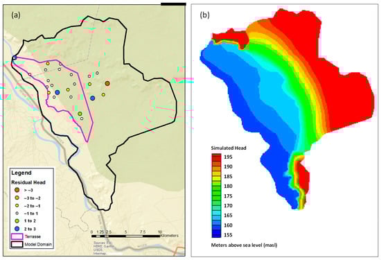
Figure 10.
Maps showing: (a) residual head, or observed groundwater level subtracted from the simulated groundwater level, in the steady-state model where larger circles show larger differences and smaller circles show smaller differences; and (b) contours of simulated head (groundwater level) shown as meters above sea level (masl) and generally following the topography.
Figure 10b shows the contours of the simulated groundwater levels (head) depicted as meters above sea level (masl). The contours generally follow the topography of the land surface, which is described above. The terrasse is located within the blue contours, while koris and escarpments are located within the red contours.
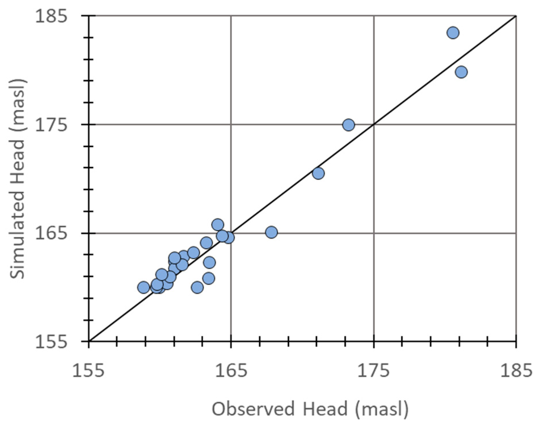
Figure 11 shows a one-to-one plot of circles that represent observed heads and the corresponding simulated heads. This type of plot can show heads as generally too high or too low and provide a sense of head distribution in a model. Below, more circles are shown clustering in the lower left corner of the plot, where head levels range from approximately 155 to 165 masl and represent the terrasse area. Head levels increase in elevation generally east of the terrasse area, and measurements are less clustered. The solid line is one-to-one; if the model were perfect, all circles would fall on the line. Though departures can be seen in the plot, there are no extreme departures or biases of heads as being generally high or low.

Figure 11.
One-to-one plot of circles that represent observed heads and the corresponding simulated heads in the steady-state model. No extreme departures or biases (generally high or low) are observed.
3.3. Flow Budget/Water Balance
Table 7 shows the flow budget for the calibrated steady-state model, as obtained from MODFLOW. Inflows are river leakage and recharge. Outflows are extraction (existing village wells), drains (wetlands), river leakage, and evapotranspiration. River leakage can be thought of as the amount of groundwater moving to or from the river and the aquifer. River leakage as an inflow is groundwater entering the aquifer from the river. River leakage as an outflow is groundwater leaving the aquifer to the river. The conceptual model used the term “discharge to the river”.
Table 7.
Flow budget for the calibrated model as obtained from MODFLOW.
The steady-state model was calibrated to match observed groundwater levels (head) to simulated head while also fitting MODFLOW-generated flow budget values to the conceptual model preliminary flow budget. The preliminary flow budget describing the inflows and outflows of the conceptual model is shown in Table 4. Estimated values for recharge, river discharge, drains, evapotranspiration, and extraction rates are described in the previous section. Phreatophyte ET and riparian ET are grouped in a lump sum named total ET. Further work and potentially a site visit are required to partition the ET and terrasse discharge terms.
It is necessary to compare the conceptual model flow budget with the MODFLOW flow budget. The total budgets for inflows and outflows for both models agree—22 × 106 m3/yr. The inflow (recharge, 22 × 106 m3/yr) and outflows (extraction, 7.2 × 10⁵ m3/yr; drains, 5.7 × 10⁶ m3/yr; and ET, 11.9 × 10⁶ m3/yr) also agree. River leakage as an outflow, described as “discharge to the river” in the conceptual model, also agrees. The MODFLOW budget indicates the presence of river leakage as an inflow, which was not estimated for the conceptual model budget. River leakage as an inflow is groundwater entering the aquifer from the river.
When developing the conceptual model, the direction and amount of groundwater flowing between the river were unclear, and an outflow amount was estimated based on other components of the flow budget. No inflow was estimated. The river leakage inflow amount indicated by MODFLOW (2.5 × 10⁴ m3/yr) is less than 0.01% of the total inflows. Despite not being estimated in the conceptual model, it is small enough to not upset the water balance. The calibrated model indicates recharge to be a larger inflow to the aquifer (22 × 106 m3/yr) than river leakage (2.5 × 10⁴ m3/yr). River leakage as an outflow is a larger value than as an inflow, which indicates a relatively smaller amount of groundwater entering the aquifer from the river (2.5 × 10⁴ m3/yr) as compared with the amount leaving the aquifer to the river (7.3 × 10⁶ m3/yr).
It is important to note that the conditions described above are likely to be time-dependent—inflow to the aquifer from precipitation is relatively larger during certain months, while inflow to the aquifer from the river is relatively larger during other months. The flow budgets for both the conceptual and calibrated steady-state models represent average conditions. On average, the steady-state model indicates the aquifer being recharged primarily from precipitation and not river water. A transient model can be used to better evaluate the seasonality and overall annual variability of river leakage, i.e., the amount of groundwater moving to or from the river and the aquifer.
4. Conclusions
While there is abundant literature describing their utility, it can be difficult to find procedures and details for numerical model construction, especially when data are scarce. The research questions for this portion of the project were how can we use existing information to develop a conceptual model and then a calibrated numerical model for a steady-state representation of a natural system where groundwater development will take place. We adressed the research questions by describing an approach to groundwater modeling beginning with data collection, through conceptual model development, and finally to a steady-state calibrated model. The resulting calibrated steady-state model is a point of departure for further modeling; approaches for transient and predictive models for Sia Kouanza will be described in subsequent publications.
The approach described details the importance of and how to understand the hydrologic and hydrogeologic setting, development of a conceptual model, understanding of the water balance, choice of numerical code, construction of a numerical model, calibration of that model, and interpretation of the calibrated steady-state model. More specifically, the team estimated recharge, evapotranspiration, discharge to wetlands, existing extraction, and river stage as components for a conceptual model. As much as possible, estimates were derived from data collected in the field by the team. When data were not available or scant, the team described other sources used and how they were validated against field data and/or analog sites. The conceptual model components were used to develop a conceptual model preliminary flow budget, which was needed for calibration.
Calibration was done by trial and error, both manually and automatically, while employing the PEST package. Three checks were used to evaluate the calibration of the Sia Kouanza model: statistical metrics, residual heads, and a flow budget (water balance). The statistical metrics methods used were ME, MAE, and RMSE. All metrics were within an acceptable range. Residual heads showed larger residuals outside the focus area of the terrasse. The flow budget generated by the model was comparable to the conceptual model flow budget.
The intent is to provide an open-access framework that can be employed in data-scarce areas where similar questions are being asked as groundwater is developed for agriculture. This intent brings us to the larger hypothesis—can we document changes and understand tipping points to support sustainable groundwater development for agriculture? This question scales beyond Sia Kouanza.
Author Contributions
Conceptualization, methodology, and software, validation, A.L., Y.N. and S.R.; formal analysis, investigation, resources, and data curation, Y.N., A.H., D.M.A. and A.G.; writing, A.L. and S.R.; project administration, Y.N., A.H., D.M.A. and D.K.; funding acquisition, D.K. All authors have read and agreed to the published version of the manuscript.
Funding
This research was funded by Millenium Challenge Corporation, grant number IR-IPD-1-SS.243-21.
Data Availability Statement
The data presented in this study are available on request from the corresponding author. The data are not publicly available because they are part of an ongoing study.
Acknowledgments
Thank you to numerous administrative assistants and technical support staff from MCC in the US and Niger.
Conflicts of Interest
The authors declare no conflicts of interest. The funders had no role in the design of the study; in the collection, analyses, or interpretation of data; in the writing of the manuscript; or in the decision to publish the results.
References
- World Food Programme. Niger Country Brief. June 2024. Available online: https://www.wfp.org/countries/niger (accessed on 25 June 2024).
- Food and Agriculture Organization of the United Nations. Integrated Production and Pest Management Programme in Africa. Available online: https://www.fao.org/agriculture/ippm/projects/niger/en/ (accessed on 1 January 2024).
- Nazoumou, Y.; Favreau, G.; Adamou, M.; Maïnassara, I. La petite irrigation par les eaux souterraines, une solution durable contre la pauvreté et les crises alimentaires au Niger? Cah. Agric. 2016, 25, 15003. [Google Scholar] [CrossRef]
- Nash, H. Groundwater Resources of the Sahel, West of Sudan. 1977. WD/CS/77/3 Institute of Geological Sciences Hydrogeological Department. Available online: https://nora.nerc.ac.uk/id/eprint/505533/ (accessed on 24 June 2024).
- Agnew, C. Water Availability and the Development of Rainfed Agriculture in South-West Niger, West Africa. Trans. Inst. Br. Geogr. 1982, 4, 419–457. [Google Scholar] [CrossRef]
- Anders, N.; Firestone, G.; Gould, W.; Versel, A.; Ware, M.; Zalla, T. Niger Irrigation Subsector Assessment, Volume One, Main Report 1984. Available online: https://pdf.usaid.gov/pdf_docs/PNAAV061.pdf (accessed on 24 June 2024).
- Goutorbe, J.P.; Lebel, T.; Dolman, A.J.; Gash, J.H.C.; Kabat, P.; Kerr, Y.H.; Monteny, B.; Prince, S.D.; Stricker, J.N.M.; Tinga, A.; et al. An overview of HAPEX-Sahel: A study in climate and desertification. J. Hydrol. 1997, 188, 4–17. [Google Scholar] [CrossRef]
- Favreau, G.; Leduc, C.; Marlin, C.; Dray, M.; Taupin, J.; Massault, M.; Le Gal La Salle, C.; Babic, M. Estimate of recharge of a rising water table in semiarid Niger from 3H and 14C modeling. Ground Water 2002, 40, 2. [Google Scholar] [CrossRef]
- Favreau, G.; Cappelaere, B.; Massuel, S.; Leblanc, M.; Boucher, M.; Boulain, N.; Leduc, C. Land clearing, climate variability, and water resources increase in semiarid southwest Niger: A review. Water Resour. Res. 2009, 45, 7. [Google Scholar] [CrossRef]
- Boucher, M.; Favreau, G.; Descloitres, M.; Vouillamoz, J.M.; Massuel, S.; Nazoumou, Y.; Legchenko, A. Contribution of geophysical surveys to groundwater modeling of a porous aquifer in semiarid Niger: An overview. CR Geosci. 2009, 341, 800–809. [Google Scholar] [CrossRef]
- Ibrahim, M.; Favreau, G.; Scanlon, B.R.; Seidel, J.L.; Le Coz, M.; Demarty, J.; Cappelaere, B. Long-term increase in diffuse groundwater recharge following expansion of rainfed cultivation in the Sahel, West Africa. Hydrogeol. J. 2014, 22, 1293–1305. [Google Scholar] [CrossRef]
- Lebel, T.; Cappelaere, B.; Galle, S.; Hanan, N.; Kergoat, L.; Levis, S.; Vieux, B.; Descroix, L.; Gosset, M.; Mougin, E.; et al. AMMA-CATCH Studies in the Sahelian Region of West-Africa: An Overview. J. Hydrol. 2009, 375, 3–13. [Google Scholar] [CrossRef]
- Galle, S.; Grippa, M.; Peugeot, C.; Moussa, I.B.; Cappelaere, B.; Demarty, J.; Mougin, E.; Panthou, G.; Adjomayi, P.; Agbossou, E.K.; et al. AMMA-CATCH, a critical zone observatory in West Africa monitoring a region in transition. Vadose Zone J. 2018, 17, 180062. [Google Scholar] [CrossRef]
- Cappelaere, B.; Vieux, B.; Peugeot, C.; Maia, A.; Séguis, L. Hydrologic process simulation of a semiarid, endoreic catchment in Sahelian West Niger. 2. Model calibration and uncertainty characterization. J. Hydrol. 2003, 279, 244–261. [Google Scholar] [CrossRef]
- Barbosa, S.; Pulla, S.; Williams, G.; Jones, N.; Mamane, B.; Sanchez, J. Evaluating Groundwater Storage Change and Recharge Using GRACE Data: A Case Study of Aquifers in Niger, West Africa. Remote Sens. 2002, 14, 1532. [Google Scholar] [CrossRef]
- Werth, S.; White, D.; Bliss, D. GRACE Detected Rise of Groundwater in the Sahelian Niger River Basin. J. Geophys. Res. Solid Earth 2017, 122, 10459–10477. [Google Scholar] [CrossRef]
- Boubacar, A.; Moussa, K.; Yalo, N.; Berg, S.; Erler, A.; Hwang, H.; Khader, O.; Sudicky, E. Characterization of groundwater—Surface water interactions using high resolution integrated 3D hydrological model in semiarid urban watershed of Niamey, Niger. J. Afr. Earth Sci. 2020, 162, 103739. [Google Scholar] [CrossRef]
- Mahaman, R.; Nazoumou, Y.; Favreau, G.; Ousmane, B.; Boucher, M.; Babaye, M.; Lawson, F.; Vouillamoz, J.; Guero, A.; Legchenko, A.; et al. Paleochannel groundwater discharge to the River Niger in the Iullemmeden Basin estimated by near- surface geophysics and piezometry. Environ. Earth Sci. 2023, 82, 202. [Google Scholar] [CrossRef]
- Nishimura, R.; Jones, N.L.; Williams, G.P.; Ames, D.P.; Mamane, B.; Begou, J. Methods for Characterizing Groundwater Resources with Sparse In Situ Data. Hydrology 2022, 9, 134. [Google Scholar] [CrossRef]
- Dike, V.N.; Addi, M.; Andang’o, H.A.; Attig, B.F.; Barimalala, R.; Diasso, U.J.; Du Plessis, M.; Lamine, S.; Mongwe, P.N.; Zaroug, M.; et al. Obstacles facing Africa’s young climate scientists. Nat. Clim Change 2018, 8, 447–449. [Google Scholar] [CrossRef]
- Rockström, J.; Williams, J.; Daily, G.; Noble, A.; Matthews, N.; Gordon, L.; Wetterstrand, H.; DeClerck, F.; Shah, M.; Steduto, P.; et al. Sustainable intensification of agriculture for human prosperity and global sustainability. Ambio 2017, 46, 4–17. [Google Scholar] [CrossRef] [PubMed]
- Zhou, Y.; Li, W. A review of regional groundwater flow modeling. Geosci. Front. 2011, 2, 2. [Google Scholar] [CrossRef]
- RTI Exploration, University of Nevada Las Vegas, Las Vegas, NV, USA. Etudes pour le développement d’outils pour la planification de la gestion des ressources en eaux souterraines et le renforcement des capacités au Niger télédétection, étude hydrogéologie, et renforcement des capacités. Unpublished Manuscript, prepared by University of Nevada Las Vegas for Millenium Challenge Account Niger. 2021. [Google Scholar]
- Funk, C.; Verdin, A.; Michaelsen, J.; Peterson, P.; Pedreros, D.; Husak, G. A global satellite-assisted precipitation climatology. Earth Syst. Sci. Data 2015, 7, 275–287. [Google Scholar] [CrossRef]
- Enemark, T.; Peeters, L.; Mallants, D.; Batelaan, O. Hydrogeological conceptual model building and testing: A review. J. Hydrol. 2019, 569, 310–329. [Google Scholar] [CrossRef]
- Reilly, T.E.; Harbaugh, A.W. Guidelines for Evaluating Ground-Water Flow Models: U.S. Geological Survey Scientific Investigations Report 2004-5038; 2004; 30p. Available online: https://pubs.usgs.gov/sir/2004/5038/PDF/SIR20045038_ver1.01.pdf (accessed on 24 June 2024).
- Anderson, M.P.; Woessner, W.W. Applied Groundwater Modeling—Simulation of Flow and Advective Transport; Academic Press, Inc.: San Diego, CA, USA, 1992; 381p. [Google Scholar]
- Helsel, D.R.; Hirsch, R.M.; Ryberg, K.R.; Archfield, S.A.; Gilroy, E.J. Statistical Methods in Water Resources: U.S. Geological Survey Techniques and Methods; Book 4, Chapter A3; U.S. Geological Survey: Reston, VA, USA, 2020; 458p. [Google Scholar] [CrossRef]
- Scanlon, B.R.; Healy, R.W.; Cook, P.G. Choosing appropriate techniques for quantifying groundwater recharge. Hydrogeol. J. 2002, 10, 18–39. [Google Scholar] [CrossRef]
- Obuobie, E.; Diekkruger, B.; Reichert, B. Use of chloride mass balance method for estimating the groundwater recharge in northeastern Ghana. Int. J. River Basin Manag. 2010, 8, 245–253. [Google Scholar] [CrossRef]
- Dettinger, M.D. Reconnaissance estimates of natural recharge to desert basins in Nevada, U.S.A., by using chloride-balance calculations. J. Hydrol. 1989, 106, 55–78. [Google Scholar] [CrossRef]
- Bromley, J.; Edmunds, W.M.; Fellman, E.; Brouwer, J.; Gaze, S.R.; Sudlow, J.; Taupin, J.-D. Estimation of Rainfall Inputs and Direct Recharge to the Deep Unsaturated Zone of Southern Niger Using the Chloride Profile Method. J. Hydrol. 1997, 188–189, 139–154. [Google Scholar] [CrossRef]
- Krautstrunk, M. An Estimate of Groundwater Recharge in the Nabogo River Basin, Ghana Using Water Table Fluctuation Method and Chloride Mass Balance. Dissertations, Professional Papers, and Capstones, University of Nevada, Las Vegas, NV, USA, 2012. [Google Scholar] [CrossRef]
- Carrier, M.A.; Lefebvre, R.; Racicot, J.; Asare, E.B. Northern Ghana hydrogeological assessment project. In Proceedings of the 33rd WEDC International Conference, Accra, Ghana, 7–11 April 2008. [Google Scholar]
- U.S. Army Corps of Engineers, Hydrologic Engineering Center (HEC). HEC Hydrologic Modeling System, User’s Manual; Version 4.0, CPD-74A; Hydrologic Engineering Center: Davis, CA, USA, 2012; Available online: https://www.hec.usace.army.mil/software/hec-hms/documentation/HEC-HMS_User’s_Manual-v4.11-20231018.pdf (accessed on 24 June 2024).
- AGRER, (Bruxelles, Belgium). Etudes D’avant-Projet Sommaire (Aps) et impact Enviral et Social (Eies) Avec Options Pour Des Etudes D’avant-Projet Detaille (Apd) et Supervision de Travaux D’Aménagements Hydro-Agricoles Dans La Région De Sia—Kouanza. Unpublished manuscript, AGRER S.A.-N.V., Prepared for Millenium Challenge Account Niger. 2020. [Google Scholar]
- Soil Conservation Service 1964. In National Engineering Handbook, Section 4, Hydrology; Department of Agriculture: Washington, DC, USA, 1964; 450p.
- Soil Conservation Service 1972. In National Engineering Handbook, Section 4, Hydrology; Department of Agriculture: Washington, DC, USA, 1972; 762p.
- Evett, S.; Kustas, W.; Gowda, P.; Anderson, M.; Prueger, J.; Howell, T. Overview of the Bushland Evapotranspiration and Agricultural Remote sensing EXperiment 2008 (BEAREX08): A field experiment evaluating methods for quantifying ET at multiple scales. Adv. Water Resour. 2012, 50, 4–19. [Google Scholar] [CrossRef]
- Richter, B.D.; Lamsal, G.; Marston, L.; Dhakal, S.; Sangha, L.; Rushforth, R.; Wei, D.; Ruddell, B.; Davis, K.; Hernandez-Cruz, A.; et al. New water accounting reveals why the Colorado River no longer reaches the sea. Commun. Earth Environ. 2024, 5, 134. [Google Scholar] [CrossRef]
- Malmberg, G. Hydrology of the valley-fill and carbonate-rock reservoirs, Pahrump Valley, Nevada-California: U.S. Geological. Surv. Water Supply Pap. 1832, 47, 1967. [Google Scholar]
- Linquist, B.; LaHue, G. Managing Rice with Limited Water. Agronomy Research and Information Center, University of California Davis Cooperative Extension. Available online: https://agric.ucdavis.edu/ (accessed on 1 March 2023).
- Pearson, C.; Lutz, A.; Huntington, J. Improving Evaporation Monitoring at Lake Hodges, California. Unpublished manuscript, Prepared for City of San Diego. 2020. [Google Scholar]
- Howard, G.; Bartam, J.; Williams, A.; Overbo, A.; Fuente, D.; Geere, J.A. Domestic Water Quantity, Service Level and Health, 2nd ed.; World Health Organization: Geneva, Switzerland, 2020. [Google Scholar]
- Niswonger, R.G.; Panday, M.; Ibaraki, M. MODFLOW-NWT, A Newton formulation for MODFLOW-2005. In U.S. Geological Survey Techniques and Methods 6–A37; US Geological Survey: Reston, VA, USA, 2011; 44p. [Google Scholar]
- Hill, M.; Tiedeman, C. Effective groundwater model calibration: With analysis of data, sensitivities, predictions, and uncertainty. In Effective Groundwater Model Calibration; Wiley: Hoboken, NJ, USA, 2007; pp. 427–455. [Google Scholar]
- National Aeronautics and Space Administration (NASA), National Imagery and Mapping Agency (NIMA), German Aerospace Center (DLR), and Italian Space Agency (ASI). Shuttle Radar Topography Mission (SRTM) Elevation Dataset: U.S. Geological Survey, Sioux Falls, South Dakota. Available online: https://earthexplorer.usgs.gov/ (accessed on 1 January 2023).
- Duffield, G.M. AQTESOLV for Windows Version 4.5 User’s Guide; HydroSOLVE, Inc.: Reston, VA, USA, 1989. Available online: http://www.aqtesolv.com/default.htm (accessed on 15 June 2023).
- Doherty, J. Calibration and Uncertainty Analysis for Complex Environmental Models; Watermark Numerical Computing: Brisbane, Australia, 2015; 227p, ISBN 978-0-9943786-0-6. Available online: www.pesthomepage.org (accessed on 15 June 2023).
- Statistics How to. Available online: https://www.statisticshowto.com/ (accessed on 1 September 2023).


Disclaimer/Publisher’s Note: The statements, opinions and data contained in all publications are solely those of the individual author(s) and contributor(s) and not of MDPI and/or the editor(s). MDPI and/or the editor(s) disclaim responsibility for any injury to people or property resulting from any ideas, methods, instructions or products referred to in the content. |
© 2024 by the authors. Licensee MDPI, Basel, Switzerland. This article is an open access article distributed under the terms and conditions of the Creative Commons Attribution (CC BY) license (https://creativecommons.org/licenses/by/4.0/).