Abstract
Neyman–Scott rectangular pulse is a stochastic rainfall model with five parameters. The impacts of initial values and optimization methods on the parameter estimation of the Neyman–Scott rectangular pulse model were investigated using both the method of moments and the method of maximum likelihood. The estimates using the method of moments were influenced by the optimization method and were sensitive to the initial values and the aggregation scale of the data. Thus, by using frequentist estimation methods, we cannot guarantee the unique values as estimates. The aim of this study is to find more reliable unique values as estimates using a Bayesian approach. In this approach, parameters are estimated from the posterior distribution, and model performance is assessed by comparing observed values with fitted values. Slice sampling within the Gibbs sampler algorithm demonstrates superior convergence and model fitting, yielding unique estimates for the model parameters. The main conclusion of this study is that Bayesian estimation methods outperform other estimation methods in terms of providing reliable and stable estimates that improve rainfall generation accuracy.
1. Introduction
In this century, the world is facing a very serious challenge of climate change and global warming. Many countries have suffered from this problem. Rainfall has a big impact on society, particularly on the environment, such as plants, water, land, etc. Moreover, floods have been the cause of the loss of many human lives. This has also affected many countries in terms of the economic and agricultural sector; because of this, studies of storm rainfall, such as the intensity of rainfall, extreme rainfall, total rainfall and heavy rains, have attracted much attention from scientists throughout the world, for example, the research carried out by [1,2,3,4,5,6].
Modeling rainfall is considered a tool for planning and managing water resources. There exist many methodologies of modeling precipitation [7,8]. Time series could be one method of modeling precipitation; however, it is not appropriate for small time scales such as hourly rainfall precipitation, since the Neyman–Scott rectangular pulse model contains a lot of parameters and due to the complexity and strong dependence upon initial conditions of the precipitation process. A stochastic approach is likely to be preferable to a purely physical model [9].
Different approaches for stochastic rainfall modeling exist; one of them is the Neyman–Scott rectangular pulse (NSRP) model, which is our concern in this study. This model has five parameters. In this paper, we investigate the method of moments and the method of maximum likelihood for NSRP parameter estimation. We found that these two methods have two main challenges. (i) Parameter estimates are highly influenced by initial values, and (ii) the optimization method has an impact on the estimates. Furthermore, Calenda et al. [9] have shown that the choice of aggregation scale time has a great influence on the estimates. Because of these challenges, classical methods of optimization are not able to provide a unique solution for parameter estimates of NSRP [10,11,12,13].
The hypothesis of this study is that the estimation of NSRP parameters is greatly impacted by two factors, the optimization method and the initial values, when using the method of moments and the MLE method. This can lead to unstable NSRP parameter estimates and affect prediction accuracy. The main goal of this study is to develop a method for NSRP parameter estimation that is not influenced by initial values or optimization. In order to overcome these challenges and obtain more reliable and unique estimates for prediction and improved accuracy, we developed a Bayesian method for the NSRP model parameter estimation. This approach uses existing information on parameters and updates it using the data to obtain the posterior distribution of which we calculated the parameter estimates. For the parameter estimation of the NSRP model, we adopted the MCMC method, specifically slice sampling within the Gibbs sampler algorithm, to obtain the posterior samples of our model parameters. The Bayesian method is not influenced by initial values, the optimization method, or the choice of aggregation scale.
To test the effectiveness of our methods, we compared the statistics calculated from observed precipitation and the statistics calculated from simulated data. We performed a comparison analysis between these two frequentist parameter estimation methods and the Bayesian approach. The primary contribution of this study is to address the issue of unstable estimates when using the method of moments and maximum likelihood estimation for NSRP parameter estimation. With this estimation method, we aim to generate unique estimates of NSRP parameters, which can, in turn, enhance the accuracy of predicted rainfall. In this study, we demonstrate our approach using hourly precipitation data from Seoul spanning the years 1972 to 2019.
This paper is structured as follows. In Section 2, we briefly describe the Neyman–Scott rectangular pulse model and the statistical properties of rainfall based on NSRP, and we discuss statistical inference of the NSRP model using classical methods and the Bayesian method. Section 3 presents the results of NSRP parameter estimation and application of NSRP to Seoul’s hourly rainfall. In Section 4, we discuss the results and we report the result of a comparative study between the methods of estimation. Finally, in Section 5, we draw concluding remarks from the study.
2. Methods: NSRP Model and Parameter Estimation Methods
2.1. NSRP Model
Neyman–Scott models are described by three independent elementary stochastic processes [1,5,6,7,8,9,10]. Briefly, these models are based on a Poisson process of storm origin, , a process that sets the origin of the events. Each storm is associated with a random number of rain cells (rectangular pulses), ; with height, which represents the rain intensity, and width, which represent the cell duration, . Figure 1 shows the schematic diagram of NSRP model. The basic formulation of the Neyman–Scott process is that the inter-arrival times of the origin of successive events are independent and identically distributed, following an exponential distribution with mean . The number of rainfall cells associated with each storm event follows a geometric or a Poisson distribution. The starting time of each rain cell, measured from the origin of the event, is exponentially distributed. The rain cell is rectangular and characterized by random radius, lifetime, and constant intensity, and both the intensity and duration of each rain cell follow an exponential distribution.
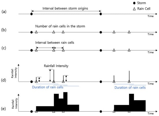
Figure 1.
Schematic diagram of NSRP model: (a) interval between storm origins, (b) number of cells in a storm, (c) interval between rain cells, (d) rainfall intensity, (e) composed rainfall events.
The precipitation intensity, , is given by the sum of the intensities of the individual active cells at time t:
where is the intensity of the rectangular pulse triggered at time u, and represents the counting stochastic process of the arrivals of the individual cells. The time series is given by:
where is the rainfall depth in the kth time interval of duration at location x.
The second-order properties of the aggregated original NSRP process are derived in [9]. In the parameter estimation of NSRP, many researchers have used classical methods such as the method of moments and maximum likelihood approaches for parameter estimation. However, these methods do not achieve unique solutions for parameter estimates. The lack of unique estimates may be due to optimization methods. During the search for an optimum solution, this may be stacked in the local optimal solution [10,14].
2.2. Frequentist Inference for NSRP Model
In this section, we estimate NSRP model parameters using classical methods such as method of moments estimation (MME) and maximum likelihood estimation (MLE). The classical methods of NSRP of estimation of parameters are based on statistical properties of precipitation. MME uses the first moment and second moment, which are mean, variance at the first scale and second scale, and covariance [1,5,6,7]. MLE is achieved by maximizing the likelihood function derived from the joint distribution of random variables and evaluated at the observed data.
2.2.1. Method of Moments
The first method of parameter estimation that we are evaluating in this paper is the method of moments. In this method, the five parameters of the NSRP model are estimated by equating the five statistical properties taken from observed data with their derived expressions from the model and solving simultaneous equations for the parameter estimates. The statistical properties of the rainfall are given below:
Hourly mean is defined by:
Hourly variance is:
Daily variance is:
Daily covariance is:
Daily correlation is:
Parameter estimates are simply obtained by minimizing the following sum of squares:
where , and stands for weight. In this study, we chose the weight to be 6. and stand for the function value from observed data and from the model, respectively.
2.2.2. Maximum Likelihood Estimation Method
Maximum likelihood estimation (MLE) is a method by which parameters are estimated by maximizing a likelihood function.
Lee et al., Kim and Kim, and Mullen [11,12,14] constructed a likelihood function from the relation of rainfall depth over an interval of length h and the method of moments estimators of NSRP. The mean, variance and covariance follow a Gaussian distribution in large samples.
where , , and stand for the variance of estimates of mean, variance and covariance, respectively.
where stand for the estimates of the mean, variance, and covariance, respectively. To minimize Equation (15), we multiplied the likelihood function by −1, and the points that minimize the likelihood function are considered parameter estimates.
Both the method of moments and method of maximum likelihood estimation require an optimization method to find estimates. Global optimization is the process of finding the minimum of a function of n parameters, with the allowed parameter values possibly subject to constraints. In the absence of constraints, the task may be formulated as , where is an objective function, and the vector represents the parameters [14]. To evaluate the influence of optimization methods on these frequentist methods, we include both deterministic and stochastic optimization methods. We investigated both methods using the following optimization algorithm: generalized simulated annealing (GenSA) is a stochastic optimization method that implements a generalized simulated annealing algorithm. It is a modification of generalized simulated annealing (GSA). This was made after finding that the distribution is not optimal for moving across the entire search space. GSA uses a distorted Cauchy–Lorentz distribution among many other simulated annealing algorithms such as fast simulated annealing (FSA), classical simulated annealing (CSA), GSA, and GenSA. GenSA was made particularly for the purpose of solving complicated nonlinear objective functions with a large number of local minima. It can also work for multidimensional real valued functions. In a comparative study with 18 other algorithms for continuous global optimization methods, it was found that GenSA performed better in terms of the quality of the solutions determined. GenSA also provides a higher average success rate compared to other algorithms. The main drawback of GenSA is searching time. It takes a long time to find the optimum, and in the case of multi-objective optimization problems, it usually finds only one solution rather than a set of solutions [13,14,15].
Differential evolution optimization (DEoptim) is a stochastic optimization method that implements differential evolution algorithms. This algorithm helps to optimize a non-convex optimization problem. It searches the global minima of the objective function between the lower and upper bound of each parameter. The solution is obtained by minimizing the objective function over the course of successive generations. DEoptim relies on the repeated evaluation of the objective function in order to move the population towards the global minimum. It works by evolving a population of candidate solutions using the alteration and selection of operators. Some advantages of this method are (1) its performance when the function has many parameters and (2) that it does not require derivatives of the objective function in the process of searching the global minimum. This is also its drawback, because it can sometimes be inefficient in the case of smooth functions, where mostly derivative-based methods are efficient; as a consequence, it can fall into a local minimum [16,17].
The Davidon–Fletcher–Powel (DFP) method is a deterministic optimization method used in unconstrained optimization, and it is the first to generalize the secant method to a multidimensional problem. This method finds a solution to the secant equation that is closest to the current estimate and satisfies the curvature condition. It is quasi-Newtonian. This algorithm forces the Hessian matrix to be symmetric and positive definite, which can greatly improve its convergence properties. This class uses first-order information only, but builds second-order information. We usually start the hessian initialized to the identity matrix and then update it at each iteration. This update maintains a positive definiteness of the Hessian matrix. This algorithm is computationally attractive and converges rapidly. Some of the problems of this method are that (1) sometimes, it fails to converge to global minimum for general nonlinear objective functions and falls into a local minimum, and (2) it is very sensitive to initial values [9,14]. The performance of a deterministic method depends on properties of the function such as convexity, boundedness, smoothness, and so on.
Hydro particle swarm optimization (hydroPSO) is a stochastic method that implements a particle swarm optimization algorithm. It is used for the global optimization of non-smooth and nonlinear functions. It is well known for its easy application in unsupervised and complex multidimensional problems that cannot be solved using deterministic algorithms. It solves a problem by having a population (swarm) of candidate solutions called particles and moving these particles around in the search for the global minimum according to a mathematical formula. This method can be simply implemented, is derivative-free, has very few algorithm parameters, and is a very efficient global search algorithm. It also has a disadvantage in its slow convergence in the refined search stage [15,16]. Due to the lack of unique estimates, a reasonable alternative method of estimation is the Bayes estimation method, by which parameters are estimated through posterior distribution.
2.3. Bayesian Inference on NSRP Model
In the previous section, we discussed both the method of moments and maximum likelihood approach for NSRP parameter estimation, and the results in Section 3 show that the estimates highly depend on initial values, and that the estimates change with the optimization method. As a consequence, there are a lack of unique solutions. To address this problem, we propose the Bayesian estimation method for NSRP parameter estimation.
2.3.1. Definition and Model Specification
The Bayesian approach directly assumes that vectors of unknown parameters are random variables that follow a specified distribution, which reflects uncertainty about these parameters [17]. In Bayesian inference, we also consider available knowledge about parameters before the sample data are analyzed. This information is known as prior distribution, denoted by . This prior information is combined with observed data information, , to calculate posterior distribution, . Bayes’ theorem illustrates the process of updating the prior to posterior distribution.
Bayes’ theorem can also be written as
where is the prior distribution, and stands for the likelihood function.
In the NSRP model structure, all parameters have positive support motivating the use of a uniform distribution as prior to parameter . The proposed minimum and maximum parameters of distributions are given in Table 1.

Table 1.
The range I of NSRP parameters (λ: storm origin, μc: random number of cells, β: cell duration, ψ: rain intensity).
We consider Equation (15) as the likelihood function. However, this likelihood is not in a closed form, and this makes it hard to derive the full conditionals. We summarized the posterior by drawing large samples from the posterior . We used the posterior distribution to compute a point estimate, which is given by the mean of samples of . After a sufficient burn-in period, the chain gradually did not depend on the initial value and converged to a unique stationary distribution. Since the full conditionals of all parameters were not in a closed form, we applied slice sampling to samples from posteriors [18]. In research carried out by [19], the authors found that gamma distribution fit outperformed other distributions in the wet season. Thus, we used gamma distribution as the prior distribution for all remaining parameters (). In addition, we used other distributions, such as log-normal distribution, inverse gamma distribution, and uniform distribution, for all parameters for prior sensitivity analysis, and the difference in the results was not significant.
2.3.2. Slice Sampling
Markov chain Monte Carlo (MCMC) is a powerful algorithm for drawing samples from a probability distribution, especially when it is complex. MCMC methods such Gibbs sampling and Metropolis Hasting are commonly used to summarize the posterior distribution. However, these two methods have some limitations in the implementation of their corresponding algorithm [19]. For example, to implement Gibbs sampling, we need full conditionals, and in Metropolis Hasting, we need to find an appropriate proposal distribution that will lead to efficient sampling. Based on the NSRP model, you might also think to implement the Metropolis Hasting within Gibbs sampling. However, this algorithm generates highly correlated samples and achieves poor convergence. In this study, we applied slice sampling within the Gibbs sampler, since it is easily implemented and can be used to sample from multivariate distribution by updating each variable at a time. In this study, we implemented a Markov chain Monte Carlo method with slice sampling with Algorithm 1.
| Algorithm 1: Algorithm of MCMC with slice sampling |
| Input: |
| 1. function proportional to density |
| 2. the current point |
| 3. the vertical level of the slice |
| 4. estimate of the typical size of a slice |
| 5. integer limiting the size of a slice to |
| Output: The interval found. |
| Repeat while |
| And |
| If then |
| else |
3. Results of Parameter Estimation
In this section, we present the results of NSRP parameter estimation using different methods. The method of moments and the method of likelihood estimation were investigated using two different initial value ranges given in Table 1 and Table A1. Both methods required optimization methods in the process of finding the estimates. We evaluated the impact of the optimization methods using DEoptim, GenSA, DFP and hydroPSo algorithms. Seoul is the largest city in South Korea with a population of approximately 10 million and is expected to suffer significant human and material damage due to summer heavy rain, so it was selected as the target site for the parameter estimation of this model. Rainfall characteristics in Seoul are concentrated during summer compared to the other seasons. Hourly summer rainfall data at Seoul were downloaded from the KMA (Korea Meteorological Administration) Open MET Data Portal site (https://data.kma.go.kr/cmmn/main.do, accessed on 1 December 2020). To investigate the influence of initial values and optimization methods on the NSRP model, historical time series data of hourly rainfall from 1972 to 2019 were used.
3.1. Results of NSRP Parameter Estimation Using MME Method
We present the results of NSRP parameter estimation using the method of moments. We evaluated this method using different initial value ranges, given in Table 1 and Table A1. For more accuracy and for the sake of comparison, we used the range of parameters proposed by [5] in Table A1, and we used different optimization methods to find the global minimum of Equation (15). The results in Table 2 show the NSRP parameter estimates using the range of initial values in Table 1. The results in Table A2 show the NSRP parameter estimates using the range of initial values in Table A1. From Table 2 and Table A2, we can see that both the initial values and optimization methods have an impact on NSRP parameter estimates.
Table 2.
Parameter estimation by MME method using range I (λ: storm origin, μc: random number of cells, β: cell duration, ψ: rain intensity).
The results in Table 2 and Table A2 indicate that two different ranges of initial values produce different parameter estimates. The results also indicate that different optimization algorithms produce different parameter estimates. One way of evaluating the model is to compare the statistics calculated from observed data and statistics calculated from simulated data. Figure 2 shows the comparison, in which the boxplot indicates the precipitation at different aggregations. The performance of optimization algorithms is ordered as follows: DEoptim, GenSA, DFP, and hydroPSO.
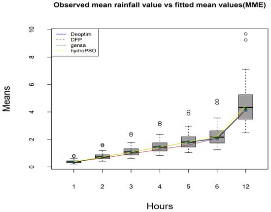
Figure 2.
A comparative graph showcases box plot of observed value, and simulated statistic at different aggregates is represented by a line. The colors correspond to the optimization algorithm used for NSRP parameter estimation using MME.
3.2. Results of NSRP Parameter Estimation Using MLE Method
In this subsection, we evaluate the method of maximum likelihood estimation of NSRP parameters using different initial values and different optimization algorithms. The two initial values are given in Table 1 and Table A1, and the optimization algorithms that we used for evaluation were GenSA, DEoptm, DFP and hydroPSO. The estimates are the global minimum of Equation (15). The results presented in Table 3 show the NSRP MLE parameter estimates using the range of initial values from Table 1. Additionally, the results in Table A3 display the NSRP MLE parameter estimates using the initial values from Table A1. Both Table 3 and Table A3 indicate that the maximum likelihood estimation (MLE) is sensitive to initial values and optimization methods.
Table 3.
Parameter estimates of NSRP by MLE using range I (λ: storm origin, μc: random number of cells, β: cell duration, ψ: rain intensity).
Table 3 and Table A3 show that the parameter estimates are highly influenced by both optimization methods and initial values. Thus, there are no unique estimates when using the maximum likelihood estimation method. To evaluate the method’s performance, we compared the statistics calculated from the observed precipitation and the statistics calculated from simulated data. We considered fitting values and observed values based on the results obtained in Table 4. Figure 3 shows the comparison, in which the boxplot indicates the precipitation at different aggregations. The performance of the optimization algorithm is ordered as follows: DEoptim, GenSA, DFP, and hydroPSO. Results from both estimation methods showed that the parameter estimates change with the optimization method, and no unique solution can be found for parameter estimates.
Table 4.
Parameter estimates of NSRP using Algorithm 1 (λ: storm origin, μc: random number of cells, β: cell duration, ψ: rain intensity).
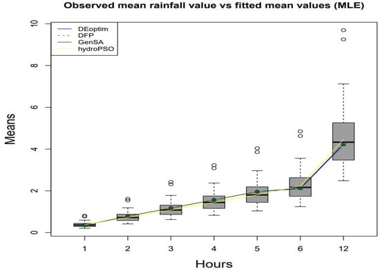
Figure 3.
A comparative graph showcases box plot of observed value and simulated statistic at different aggregates is represented by a line. The colors correspond to the optimization algorithm used for NSRP parameter estimation using MLE.
3.3. Results of NSRP Parameter Estimation Using Bayesian Estimation Method
In Bayesian estimation, it is very important to check whether the sampling achieves convergence and stationary distribution. In this study, we applied different convergence diagnostic methods such as trace plots for one single chain and trace plots for multiple chains [20,21,22,23]. Three MCMC chains with different initial values mixed well within 10,000 iterations after 5000 burn-ins, and they converged to the same range of value of each parameter, which is also the reason why Bayesian estimation provides a reliable estimate. Dependency between samples is a problem, since it delays the convergence. Therefore, we checked autocorrelation plots for the posterior samples for each parameter. The autocorrelation in all posterior samples is very small. In addition to that, we performed some standard tests of the stationarity of MCMC samples such as Geweke and Gelman–Rubin plots. Both visual and numerical diagnostic methods indicate a good MCMC convergence. The fact that three different chains of each parameter with different initial values converge indicates that the parameter estimates do not depend on initial values. Thus, this method produces a unique solution for parameter estimates. We evaluated models by comparing the statistics calculated from the observed precipitation and the statistics calculated from simulated data using different parameter estimation methods in Table 5.
Table 5.
Observed and fitted values obtained using different estimation methods at different time scales.
In this section, we compare the method of moments estimation, maximum likelihood estimation and Bayesian estimation (posterior means) approaches for NSRP parameters. First, we compared the fitted values produced using these methods and the actual values, and secondly, we compared them by generating precipitation using the estimates obtained by these methods; then, we compared the statistics of generated rainfall and statistics obtained from actual rainfall.
3.4. Parameter Estimate Evaluation Methods
In this section, we propose a method of evaluating the performance of different NSRP parameter estimates. This method is based on generating synthetic rainfall using the estimates and calculating statistics from generated rainfall. Algorithm 2 provides steps for generating synthetic rainfall.
| Algorithm 2: Algorithm for generating a synthetic rainfall |
|
|
|
|
|
Note that we compared MME methods with different optimization algorithms with the Bayesian method. We used the range of initial values given in Table A1. The results in Table 6 show that the Bayesian method produces the closest estimate to true.
Table 6.
Results from Algorithm 2 (comparative study between estimates obtained from different method with true parameters).
4. Discussion
In this study, we investigated methods of parameter estimation for the NSRP model and evaluate the method of moments estimation and the method of maximum likelihood estimation using different optimization algorithms with different initial values. The four optimization algorithms considered in this paper are DEoptim, GenSA, DFP, and hydroPSO. All these algorithms produce a significant heterogeneity in estimates. The results indicated that initial values highly influence the estimates, which vary with the choice of optimization algorithm. Consequently, both frequentist estimation methods failed to produce reliable estimates, as they all depend on optimization techniques in the estimation process. We evaluated the estimation method by comparing statistics of observed data with fitted values. The accuracy of the estimates produced by different optimization methods is ordered as below: DEoptim, GenSA, DFP, and hydroPSO.
It is also important to note that these methods do not only produce different estimates but they are also different in terms of computing time. Our major contribution is the development of a Bayesian statistical approach to the problem of NSRP parameter estimation that guarantees reliable estimates. A Markov chain Monte Carlo (MCMC) method, specifically slice sampling within the Gibbs sampler algorithm, was developed for parameter estimation. Different convergence diagnostic measures such as density plot, autocorrelation plot, Geweke plot and Gelman–Rubin plot (multichain plot) were applied to all posterior samples, and all of them indicated good convergence. The Bayesian estimation method was able to provide reasonably and good reliable solutions as parameter estimates, in terms of convergence and model fitting. In this case, the estimates were not influenced by initial values. A comparison between frequentist estimation methods and Bayesian estimation methods was also considered, and Bayesian estimates were found to be consistent and more accurate in terms of model fitting. The application of Bayesian estimation methods for parameter estimation yields unique estimates that enhance precipitation prediction accuracy, rendering these results more reliable due to their stable estimates. Comparatively, unstable estimates identified in other studies hinder result reproduction and lead to prediction variations.
Additionally, we introduced a simulation method to evaluate model performance, involving the generation of synthetic rainfall using the estimates and derivation of statistics from the generated rainfall. Our study demonstrates that the Bayesian estimation method can produce NSRP parameter estimates unaffected by scale. The resulting rainfall statistics closely align with actual rainfall in Seoul, indicating the suitability of this method for parameter-estimation modeling. However, the Bayesian estimation method has its limitations. The drawback of this method lies in its computational expense, particularly when handling large datasets and numerous simulations, as well as the challenge of selecting the appropriate prior.
In the present study, the results of NSRP Bayesian estimation method were compared with existing results in [11,16], and while the estimates were comparable, our method produced reproducible and unique estimates. For future research, it is imperative to assess the performance of these methods on other datasets with varying aggregates and quantify the impact of unstable estimates. Furthermore, additional testing of the model’s applicability for rainfall in other seasons, catchment areas, and different time scales is recommended. The performance of observed data should be verified by comparing them with data generated through simulation.
5. Conclusions
In conclusion, the results of this study unequivocally establish the efficacy of the Bayesian estimation method in producing NSRP parameter estimates that are both unique and highly reliable. Significantly, our findings indicate that this method shows great promise in enhancing the precision and dependability of NSRP Bayesian parameter estimates, which is crucial for engineering applications reliant on accurate rainfall data for design and planning purposes. The rainfall statistics derived from the estimates closely correspond with the actual rainfall in Seoul, affirming the suitability of this method for NSRP parameter estimation. Further investigation and validation of this approach within rainfall modeling have the potential to drive substantial progress in rainfall estimation and its impact on engineering design and infrastructure planning.
Author Contributions
Conceptualization, P.N., K.E.L. and G.K.; schematic diagram of the methodology presented in this study, P.N. and G.K.; methodology, P.N., K.E.L. and G.K.; software, P.N.; validation P.N. and G.K.; formal analysis, P.N., K.E.L. and G.K.; investigation, P.N., K.E.L. and G.K.; resources, G.K.; data curation, G.K.; writing—original draft preparation, P.N.; writing—review and editing, P.N. and K.E.L.; visualization, P.N., K.E.L. and G.K.; supervision, K.E.L. and G.K.; project administration, G.K.; funding acquisition, G.K. All authors have read and agreed to the published version of the manuscript.
Funding
This research was supported by a grant (RS-2022-ND634021(2022-MOIS61-002)) for the development Risk Prediction Technology of storm and Flood for Climate Change based on Artificial Intelligence funded by Ministry of Interior and Safety (MOIS, Korea).
Data Availability Statement
The data that support the findings of this study are available from the corresponding author upon reasonable request.
Conflicts of Interest
The authors declare no conflicts of interest.
Appendix A
Table A1.
The range II of NSRP parameters (λ: storm origin, μc: random number of cells, β: cell duration, ψ: rain intensity).
Table A1.
The range II of NSRP parameters (λ: storm origin, μc: random number of cells, β: cell duration, ψ: rain intensity).
| Parameters | |||||
|---|---|---|---|---|---|
| Minimum | 0.001 | 2.00 | 0.01 | 0.10 | 0.30 |
| Maximum | 0.050 | 100 | 0.50 | 10.0 | 15.0 |
Table A2.
Parameter estimate by MME method using range II (λ: storm origin, μc: random number of cells, β: cell duration, ψ: rain intensity).
Table A2.
Parameter estimate by MME method using range II (λ: storm origin, μc: random number of cells, β: cell duration, ψ: rain intensity).
| Parameters | |||||
|---|---|---|---|---|---|
| DEoptim | 0.0144 | 26.1241 | 0.4636 | 4.9650 | 4.5400 |
| GenSA | 0.0145 | 33.8982 | 0.5000 | 8.9875 | 6.2956 |
| DFP | 0.0174 | 11.7683 | 0.4510 | 2.4031 | 4.0359 |
| hydroPSO | 0.0048 | 72.9754 | 0.1355 | 2.1073 | 2.0771 |
Table A3.
Parameter estimates of NSRP by MLE using range II (λ: storm origin, μc: random number of cells, β: cell duration, ψ: rain intensity).
Table A3.
Parameter estimates of NSRP by MLE using range II (λ: storm origin, μc: random number of cells, β: cell duration, ψ: rain intensity).
| Parameters | |||||
|---|---|---|---|---|---|
| DEoptim | 0.0104 | 10.8663 | 0.1572 | 1.3414 | 4.1866 |
| GenSA | 0.0107 | 34.8706 | 0.2538 | 7.4592 | 6.9941 |
| DFP | 0.0100 | 8.07160 | 0.1288 | 0.9044 | 3.9175 |
| hydroPSO | 0.0105 | 10.2974 | 0.1532 | 1.6907 | 5.5753 |
References
- Cowpertwait, P.S.P.; Kilsby, C.G.; O’Connell, P.E. A spatial-time Neyman-Scott model of rainfall: Empirical analysis of extremes. Water Resour. Res. 2002, 38, 1131. [Google Scholar] [CrossRef]
- Martinez, M.D.; Lana, X.; Burgueño, A.; Serra, C. Spatial and temporal daily rainfall regime in Catalonia NE Spain derived from four precipitation indices, years 1950–2000. Int. J. Climatol. 2007, 27, 123–138. [Google Scholar] [CrossRef]
- Aravena, J.C.; Luckman, B.H. Spatiotemporal rainfall patterns in southern South America. Int. J. Climatol. 2009, 29, 2106–2120. [Google Scholar] [CrossRef]
- Sen Ropy, S. A special analysis of extreme hourly precipitation patterns in India. Int. J. Climatol. 2008, 29, 345–355. [Google Scholar] [CrossRef]
- Burguenu, A.; Matinez, M.D.; Liana, X. Statistical contribution of the daily rainfall regime in Catalonia (northeastern Spain) for the years 1950–2000. Int. J. Climatol. 2005, 28, 1381–1403. [Google Scholar] [CrossRef]
- Rodriguez, I.; Gupta, V.K.; Waymire, E. Scale considerations in the modeling of temporally rainfall. Water Resour. Res. 2011, 20, 1611–1619. [Google Scholar] [CrossRef]
- Sung, J.H. Analysis of extreme rainfall characteristics in 2022 and projection of extreme rainfall based on climate change scenarios. Water 2023, 15, 3986. [Google Scholar] [CrossRef]
- Dubey, S.K.; Kim, J.J.; Hwang, S.; Her, Y.; Jeong, H. Variability of extreme events in coastal and inland areas of South Korea during 1961–2020. Sustainability 2023, 15, 12537. [Google Scholar] [CrossRef]
- Calenda, G.; Napolitano, F. Parameter estimation of Neyman-Scott process for temporal point rainfall simulation. J. Hydrol. 1999, 225, 45–66. [Google Scholar] [CrossRef]
- Cowpertwait, P.S.P.; O’Connell, P.E.; Metcalfe, A.; Mawdsley, J. Stochastic point process modeling of rainfall. I. Single site fitting and validation. J. Hydrol. 1996, 175, 17–46. [Google Scholar] [CrossRef]
- Lee, J.J.; Kim, Y.G. A spatial analysis of Neyman-Scott rectangular pulses model using an approximate likelihood function. J. Korean Data Inf. Sci. Soc. 2016, 27, 1119–1131. [Google Scholar]
- Kim, Y.; Kim, D.H. An approximate likelihood function of spatial correlation parameters. J. Korean Data Inf. Sci. Soc. 2015, 45, 276–284. [Google Scholar] [CrossRef]
- Xiang, Y.; Gubian, S.; Suomela, B.; Hoeng, J. Generalized simulated annealing for efficient global optimization: The GenSA Package for R. R J. 2013, 5, 13–28. [Google Scholar] [CrossRef]
- Mullen, K.M. Continuous global optimization in R. J. Stat. Softw. 2004, 60, 1–45. [Google Scholar]
- Scrucca, L. GA: A package for genetic algorithms in R. J. Stat. Softw. 2013, 53, 1–37. [Google Scholar] [CrossRef]
- Kim, G.; Cho, H.; Yi, J. Parameter estimation of the Neyman-Scott rectangular pulse model using a differential evolution method. J. Korean Soc. Hazard Mitig. 2012, 12, 187–194. [Google Scholar] [CrossRef][Green Version]
- Ardia, D.; Mullen, K.M.; Peterson, B.G.; Ulrich, J. DEoptim: Differential evolution in R, R package version. J. Stat. Softw. 2013, 2, 2. [Google Scholar]
- Neal, R.M. Slice sampling. Ann. Stat. 2003, 31, 705–741. [Google Scholar] [CrossRef]
- Gelman, A. Inference and Monitoring Convergence in Markov Chain Monte Carlo in Practice; Gilks, W.R., Richarson, S., Spiegelhalter, D.J., Eds.; Chapman and Hall: London, UK, 1996; pp. 131–143. [Google Scholar]
- Gamerman, D.; Lopes, H.F. Markov Chain Monte Carlo, Stochastic Simulation for Bayesian Inference; Chapman & Hall/CRC: Boca Raton, FL, USA, 2006; pp. 320–342. [Google Scholar]
- Gelman, A.; Rubin, D.B. Inference from iterative simulation using multiple sequence. Stat. Sci. 1992, 7, 457–472. [Google Scholar] [CrossRef]
- Geyer, C.J. Practical Markov Chain Monte Carlo. Stat. Sci. 1992, 7, 473–483. [Google Scholar] [CrossRef]
- Cowles, M.K.; Carlin, B.P. Markov Chain Monte Carlo convergence diagnostic: A comparative review. J. Am. Stat. Assoc. 1996, 91, 883–904. [Google Scholar] [CrossRef]


Disclaimer/Publisher’s Note: The statements, opinions and data contained in all publications are solely those of the individual author(s) and contributor(s) and not of MDPI and/or the editor(s). MDPI and/or the editor(s) disclaim responsibility for any injury to people or property resulting from any ideas, methods, instructions or products referred to in the content. |
© 2024 by the authors. Licensee MDPI, Basel, Switzerland. This article is an open access article distributed under the terms and conditions of the Creative Commons Attribution (CC BY) license (https://creativecommons.org/licenses/by/4.0/).