Abstract
Continuous measurements of soil moisture in the deeper parts of the unsaturated zone remain an important challenge. This study examines the development of an integrated system for the continuous and 3-D monitoring of the vadose zone processes in a cost- and energy-efficient way. This system comprises TDR, ERT and GPR geophysical techniques. Their capacities to adequately image subsurface moisture changes with continuous and time-lapse measurements are assessed during an artificial infiltration experiment conducted in a characteristic urban site with anthropogenic fills and much compaction. A 3-D array was designed for each method to expand the information of a single TDR probe and obtain a broader image of the subsurface. Custom spatial TDR probes installed in boreholes made with a percussion drilling instrument were used for soil moisture measurements. Moisture profiles along the probes were estimated with a numerical one-dimensional inversion model and a standard calibration equation. High conductivity water used during all infiltration tests led to the detection of the flow by all techniques. Preferential flow was present throughout the experiment and imaged sufficiently by all methods. Overall, the integrated approach conceals each method’s weaknesses and provides a reliable 3-D view of the subsurface. The results suggest that this approach can be used to monitor the unsaturated zone at even greater depths.
1. Introduction
The unsaturated, or vadose, zone is the part of the subsurface that lies on top of the water table, where numerous key processes that govern the energy and mass transfer between the atmosphere and the subsurface take place [1]. Measuring the hydraulic properties of the vadose zone in an accurate way is vital in a broad range of applications that extend from water resources management and agriculture [2,3] to meteorology and geotechnical studies. Monitoring, predicting and modeling water storage, fluxes and solute transport through that zone can ameliorate risk assessment and treatment planning of contaminated areas and provide an estimate of percolation and groundwater recharge rates [4,5]. Precise and methodical monitoring of the downward motion of the waterfront during an artificial or natural infiltration event is pivotal in quantifying and modeling aquifer recharge, waste disposal leakage and artificial recharge basin efficiency [6]. The unsaturated zone can also regulate the available water for irrigation, act as a zone of filtration for contaminants released on the ground surface through chemical, biological and physical processes and play a pivotal role in slope stability and flood management [1].
Monitoring and characterizing the vadose zone is a demanding operation, especially when the research has to reach important depths, because of the complex, highly dynamic and non-linear nature of transport processes, such as precipitation, infiltration and evapotranspiration. Temporally and spatially varying soil parameters and hydraulic properties lead to great soil heterogeneity [7,8,9]. Comprehensive reviews regarding flow processes, mechanisms and definitions of the unsaturated zone can be found in [10,11,12,13].
The shallow unsaturated zone can be sufficiently mapped with relatively high resolution and spatial coverage with surface geophysical methods. However, these techniques are less efficient for monitoring the deeper parts of the unsaturated zone since their resolution and reliability diminish with increasing depth. For these parts, boreholes are the most appropriate and common way to attain adequate vertical resolution for quantitative hydrological portrayal, either via direct sampling or as ingress points for the indirect techniques, but the cost and labor required are many times prohibitive [1].
TDR has been a widely accepted indirect electromagnetic method for soil moisture measurements, both in the laboratory and the field, for more than 5 decades [14,15,16,17]. It measures the travel time and propagation velocity of a high-frequency electromagnetic signal along two- or three-parallel metal rod probes that act as transmission lines [18,19]. The travel time strongly depends on the bulk dielectric permittivity of the soil surrounding the probe, which is highly influenced by its amount of moisture. Empirical and semi-theoretical calibration equations and models are used to relate the dielectric permittivity measured to soil volumetric water content [17,20]. The main asset of TDR is that provides continuous, rapid, automated and accurate measurements of apparent relative dielectric permittivity and bulk soil conductivity in the same sample volume because of its high-frequency operation [21,22].
TDR and point-measurement techniques measure a small volume of soil, confined to a few centimeters around the probes, which makes them sensitive to air gaps and macropores, resulting in constrained representativeness and elevated uncertainty for field-scale spatial coverage [23,24]. Establishing a larger network of many point-scale sensors can be costly, labor-intensive and impractical [25,26,27,28]. Moreover, these techniques involve drilling and installing probes, which disturb the soil structure, leading to less representative soil conditions and water content measurements [29]. The biggest constraint of TDR is its inability to measure the apparent relative permittivity of highly saline soils accurately, where it systematically overestimates the water content [30,31].
Most TDR investigations for soil moisture determination and water flux monitoring have been limited to the shallow vadose zone, in the vicinity of the rhizosphere [6,32,33,34,35,36]. During the last 20 years, various TDR probes have been designed to achieve a WC profile at depths greater than a few centimeters from the surface. Kallioras et al. (2016) [6] state that ‘a holistic investigation of the water flux through the unsaturated zone, as well as the monitoring of the wetting front down to significant depths through the unsaturated zone, demands the installation of spatial TDR probes, which penetrate significantly deep down through the unsaturated zone’. Spatial TDR has been named the technology of soil moisture profile measurements [37]. Ref. [38] introduced a methodology for deep vadose zone monitoring using TDR probes with flexible waveguides attached to a flexible sleeve. Ref. [39] developed a probe called TAUPE for use with common TDR instruments and for spatial and vertical soil moisture profile measurements. Ref. [40] used custom and commercial inflatable TDR probe packers, lowered into a borehole, for the monitoring of a 14 m thick vadose zone. Ref. [41] presented a new technique for the installation of access-tube TDR probes and the calibration of soil water profiling measurements in deep heterogeneous soils, while [42] designed several cylindrical access tubes, with surface-mounted waveguides and varying geometrical characteristics, for in situ soil moisture measurements. Ref. [43] developed a technique for soil sampling and horizontal installation of three-rod TDR probes in the walls of vertical or angled boreholes, to a depth of up to 10 m, contributing to the daunting task of characterizing the deeper vadose zone. Refs. [37,44,45,46,47,48] developed and used several spatial probe designs and inversion algorithms for the monitoring and reconstruction of transient soil moisture profiles, both in the field and in the laboratory. Ref. [6] implemented a series of field techniques for investigating soil moisture profiles at significant depths of the unsaturated zone, utilizing specially designed probes.
The development of spatial TDR probes for the accurate determination of soil moisture profiles at depths greater than a few centimeters is of the utmost importance for many groundwater investigations, such as monitoring and mapping solute transport processes and aquifer contamination [49,50,51]. Comprehensive reviews on measurement principles, calibration equations and applications of TDR in porous media can be found in [23,52,53,54,55].
To fill the gap between point-scale and remote sensing methods, non-invasive geophysical techniques have been deployed for more than twenty years to investigate hydrological processes and map soil moisture variabilities in the unsaturated zone with improved spatial characterization and field representativeness compared with point methods [11,28,56,57,58,59,60,61]. These techniques lead to a better understanding of water flow and storage in the soil during processes such as infiltration [62,63,64,65,66], transport of tracers [67,68,69] and plume dissemination [70].
Ground penetrating radar (GPR) and electrical resistivity tomography (ERT) have been the most common geophysical methods in hydrological studies over the last decades. GPR is an electromagnetic technique, akin in theory to TDR, that generates a high-frequency electromagnetic pulse (1 MHz–1 GHz) and measures the propagation velocity of the transmitted and reflected wave into the ground [26]. The fairly high spatial resolution of the method and the strong link between propagation velocity and soil bulk dielectric permittivity, which in turn is strongly associated with soil moisture [17], are the reasons for the wide acceptance of GPR for time-lapse soil moisture estimation and mapping of water distribution in hydrological studies [56,58,71]. In addition, the non-invasive nature and bigger sampling volume of GPR make it less liable to air gaps and macropores than TDR [23]. Similar to TDR, when conductive materials, like saline and clay soils that exceed 1 dS/m are present, the signal is attenuated and the wave penetration depth is restricted to a few meters [60,72].
Several ground-based and cross-borehole GPR studies have been conducted over the last two decades to monitor water movement in the vadose zone during natural and forced infiltration events and infer the hydraulic properties of the subsurface [28,64,65,73,74,75,76,77,78,79,80,81]. An extensive review of GPR in groundwater studies during the last twenty years can be found in [82].
ERT is probably the most utilized non-invasive geophysical technique for groundwater investigations. Typically, a pair of electrodes injects electrical current into the ground while another pair measures the resulting voltage difference within the generated electric field. From that difference, via forward modeling and inversion techniques, the subsurface electrical resistivity allocation can be inferred [83], which is the inverse of electrical conductivity and expresses the intrinsic capacity of a material to resist the flow of electrical current through its body [11,61].
ERT can provide high-resolution subsurface images and automated data acquisition. However, mostly in unsaturated conditions, electrical resistivity profiles are dependent not only on soil water content but also on parameters such as pore water salinity, grain size, temperature and clay content, which complicate vadose zone investigations [28,58]. Conducting time-lapse measurements is presumably the best way to minimize the impacts of these parameters and is a great tool for monitoring water infiltration since it can minimize the effect of lithology and other factors that affect resistivity. Therefore, temporal SWC changes can be mapped with high accuracy and, for this reason, ERT has been applied in numerous field-scale hydrological studies in the vadose zone over the last decades [84], which include tracer and solute transport monitoring during controlled infiltration experiments [65,69,75,85,86,87,88,89,90,91], monitoring of soil water flow patterns under different irrigation scenarios [29,92,93,94], contaminant, tracer and water plume monitoring during snowmelt infiltration [4,95,96,97] and rainfall and fresh water plume infiltration monitoring [9,98,99]. More insight into the use of ERT in hydrogeology can be found in [100].
The importance of time-lapse geophysical data in hydrological studies is highlighted in [7,77,89,101,102,103,104], while [105,106,107] used this technique to study complex infiltration and recharge processes [58].
The aim of this study is to develop an integrated system for the 3-D, real-time, continuous and in situ monitoring of soil moisture variations and hydrological processes in the shallow vadose zone during an artificial infiltration experiment. The system comprises TDR with custom spatial probes, near-surface ERT and GPR, as well as a percussion drilling and soil sampling technique for heterogeneous soils. TDR is selected as a reference method for accurate soil moisture estimations in the vicinity of the probes and it is coupled with ERT and GPR for a more spatial image of the water fluxes in the unsaturated zone during and after infiltration. This work evaluates the advantages and limitations of these geophysical techniques in mapping the unsaturated zone processes with time-lapse measurements and examines the potential of this system for continuous and accurate soil water content measurements at depths greater than a few meters from the ground surface, which is a major remaining issue of unsaturated zone hydrology. Converting geophysical tomograms into quantitative estimates of water content is beyond the scope of this paper since a qualitative cross-check among TDR, ERT and GPR meets the requirements of this study. The infiltration experiment was conducted at an experimental field site on the NTUA campus in Athens, Greece.
2. Materials and Methods
2.1. Infiltration Experiment Setup
An infiltration setup was designed and installed at the experimental field site to monitor, in a 4D, spatiotemporal, real-time and continuous fashion, the soil moisture variations and hydrological processes in the unsaturated zone during a forced-infiltration experiment, implementing an integrated system comprising TDR, GPR and ERT, as well as, hand-operated auger, percussion drilling and soil sampling sets. This site was selected because it is accessible and characteristic of urban conditions, mainly composed of gravel, sand and anthropogenic fills, such a, rubbles, bricks and dashes of mortar. The soil lacked cohesion and consistency in its structure, indicative of some kind of disturbance during filling and construction works.
In the center of a 7 m × 8 m plot, a cylindrical hole with a diameter of 57 cm and a depth of 20 cm was excavated, and a double-ring infiltrometer was installed, where the water was going to infiltrate the soil at a rate of about 1 L/min, after a constant infiltration rate was achieved. A 600 L tank served as the source of water, while one ballcock was installed in each one of the rings to control the water flow and achieve a steady inflow. The outer ring of the infiltrometer had a diameter of 57 cm and a height of 25 cm, while the inner one had a diameter of 32 cm and a height of 25 cm. These dimensions are literature standard design for double-ring infiltrometers. Both rings were inserted 5 cm vertically into the soil to minimize the lateral spreading of the water and achieve a vertical initial infiltration, while no part of the rings projected from the surface, as the GPR grid lines transected the hole. Both rings were made of plastic to avoid interference with GPR and ERT measurements. A custom TDR probe with a length of 1 m was installed vertically in the center of the inner ring (Figure 1).
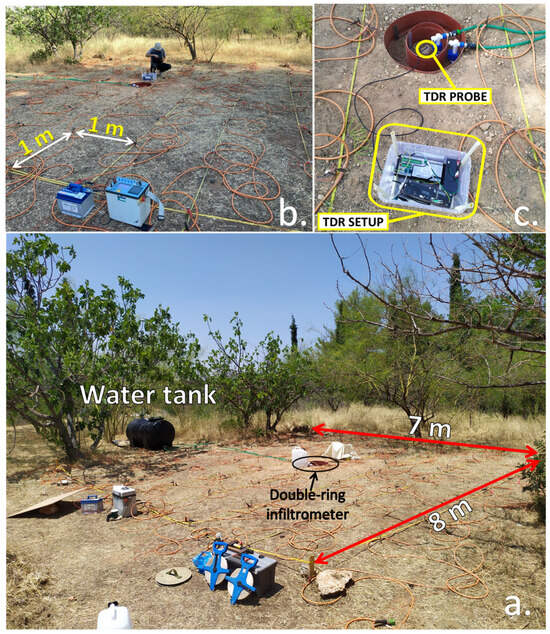
Figure 1.
(a) The 7 m × 8 m field plot of the infiltration experiment. (a,b) The 3-D ERT survey plot with 72 electrodes and 1.0 m electrode spacing. (c) The double-ring infiltrometer in the center of the plot where the water infiltrated the soil, the central TDR probe installed in the center of the double-ring setup and the integrated Campbell Scientific TDR monitoring setup comprising a pulse generator (TDR100), a datalogger (CR800) and a multiplexer (SDMX50) (Manufacturer: Campbell Scientific Ltd., Loughborough, UK).
The hydrogeophysical survey was conducted in the summer of 2022 and consisted of four phases. After the end of each phase, a period of three weeks was allowed so that the plot could dry as much as possible under the influence of the scorching heat and the infiltration test could be repeated with similar conditions. The water infiltration process lasted roughly four hours, and a volume of about 500 L of water infiltrated the soil during each phase of the experiment. Despite the high environmental temperatures, the evaporation of water was considered insignificant because of the small surface of the infiltrometer setup (about 0.26 m2) and the short duration of the experiment.
The first phase was conducted in July and included the deployment of the TDR technique with the use of a single probe installed in the center of the plot. The second phase comprised a 3-D TDR array with four more probes, identical to the original, installed two meters apart from the central probe in a cruciform array. The purpose of this phase was to investigate if we could obtain important information with point measurements regarding the direction of the infiltrating water and how the shallow unsaturated zone behaves. We wanted to test if the single-probe system could be expanded into a spatial grid and detect, in a more spatial manner, what ERT and GPR could detect. A degree of agreement among the TDR, ERT and GPR results would validate the development of an integrated, high-accuracy and powerful system for the monitoring of the infiltrating front, benefitting from the strong points of each method. Appropriately combining the continuous, automated and high-accuracy soil moisture measurements by TDR and similar dielectric sensors with the spatial coverage of conventional geophysical techniques would be an important leap forward in the monitoring and understanding of the vadose zone processes, such as infiltration and evapotranspiration and their non-linear relationship with soil moisture.
The third and fourth phases included the deployment of ERT and GPR, respectively, based on the TDR results from the first two phases. During the third phase, a rectangular 7 m × 8 m ERT survey plot with a total of 72 electrodes (8 lines with 9 electrodes each) with 1.0 m electrode spacing was designed for 3-D resistivity measurements of the underground during the infiltration experiment (Figure 1). The pole–dipole array was preferred, and the furthest electrode was situated at a 100 m distance from the plot. The position of that electrode was measured with GPS and factored into the calculation of apparent resistivities [108]. The pole–dipole array was chosen for its enhanced lateral and vertical resolution of the subsurface, which contributed to a better monitoring of the flows and paths of the infiltrating water. A total of ten resistivity measurements were conducted. Each one lasted about 24 min, and the whole experiment lasted more than four hours. The first measurement was conducted before the infiltration started, in dry conditions, to obtain a glimpse of the subsurface in its natural state and obtain a reference image on which the interpretation of the subsequent images was based. The other nine measurements were conducted during infiltration and until the end of it.
The fourth phase was designed to cross-check the results of the first three phases and provide additional insight into the hydrological processes of the shallow part of the vadose zone. Based on the water flow indicated by TDR and ERT, four intersecting GPR grid lines were designed to detect the same movement in 2-D and 3-D mode. Each line crossed the center of the grid, where the double-ring infiltrometer was installed, to capture water movement in any direction. The results from GPR transect line 4 were expected to be of great importance since that was the main direction of the infiltrating water, as indicated by ERT and TDR. A total of fourteen GPR measurements were conducted during infiltration. Four more were conducted during the first hour after infiltration stopped to monitor how the waterfront and the unsaturated zone settled and behaved, while a single measurement was conducted before infiltration to image the initial state of the subsurface and moisture remnants from the previous phases. With these four phases, the spatiotemporal movement of water and the continuous and high-accuracy spot water content profiles were obtained using time-lapse ERT, GPR and TDR measurements.
The installation of the five spatial custom probes for the first and second phases of the experiment required drilling vertical boreholes with a diameter of 7 cm and a depth of 1.2 m. Initially, drilling was carried out with a hand-operated auger, with a diameter of 7.5 cm, by Eijkelkamp (Royal Eijkelkamp, Giesbeek, The Netherlands). However, after a depth of 60 cm, hand-operated augering was not possible because of the presence of large gravels, boulders and rubbles that tended to block the rotation of the instrument. From that depth onwards, a percussion drilling set by Royal Eijkelkamp, ideal for urban areas and soils with bricks and large stones, was used. The gasoline-powered percussion hammer utilized was Makita HM 1400 (Makita U.S.A., Inc., La Mirada, CA, USA), and the maximum drilling diameter was 7.5 cm. Even in this case, the maximum depth achieved did not exceed 1.3 m. After that depth, the gouge was filled with large stones, and its extraction was almost impossible because of the enormous friction generated. That was the determining factor in deciding on the length of the custom TDR probes, which was limited to one meter for this experiment. During all drilling stages, soil sampling was conducted, and soil cores were retrieved every 20 cm, up to a depth of 1.2 m, for soil profile description and classification.
This work tries to expand the use of TDR in a more spatial array and assess the capacity of ERT and GPR to monitor spatial soil moisture changes. The three techniques have different sensing volumes and measurement resolutions. The drilling setup flexibility, ease of transport and performance are also evaluated. The final takeaway considers the developed system as capable or not for monitoring and mapping the water fluxes and hydrological processes at greater depths of the vadose zone, which is invaluable information for several processes and applications, as is the quantification of the underlying aquifer recharge [6].
2.2. Infiltration Rate and Grain Size Analysis
To better interpret TDR soil moisture profiles and geophysical tomograms, several field and laboratory tests were conducted to calculate the average infiltration rate and grain size profile of the experimental field site. For the determination of the infiltration rate, double-ring and single-ring infiltrometer tests were executed in different spots of the plot (Figure 2). As [9] states, ‘infiltration is the entry of water into the soil from the ground surface and the associated flow away from the surface within the unsaturated zone [109]. The speed of this movement is called the infiltration rate, and its unit is length per time. In the beginning, the infiltration rate, or infiltration capacity (the maximum rate at a given time), in dry soils is very high because of considerable matrix suction but then it declines as time passes because of the saturation of the shallower parts of the soil and the decrease in capillary suction until it reaches an almost steady rate. This rate nearly equals the saturated hydraulic conductivity and presents the highest value of conductivity. In unsaturated soils, the pores are partially filled with air and do not transmit water as fast.
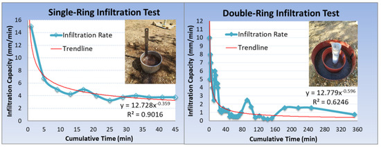
Figure 2.
The single-ring and double-ring infiltrometer setups and their respective infiltration curves.
The double-ring infiltrometer installed in the center of the plot was used to construct the first infiltration curve. The outer and inner rings were constantly filled with water for more than 6 h, maintaining a water level inside the rings between 5 and 10 cm. The water level was recorded at certain times, and the respective infiltration curve was constructed (Figure 2). About 600 L of water infiltrated the soil during the test.
The main advantage of the double-ring infiltrometer, in contrast with the single-ring infiltrometer, is that the water infiltrating the soil from the outer ring acts as a buffer wall that confines the lateral dissemination of the infiltrating water from the inner ring and forces it to infiltrate mostly vertically in the upper parts of the infiltrating zone, which generally leads to a more representative infiltration curve.
The single-ring infiltrometer is also used in the literature and is considered a good supplementary or alternative technique since the double-ring infiltrometer takes a lot of time and water. For the determination of the single-ring infiltration curve, a metal cylinder with a diameter of 8 cm and a height of 20 cm was driven 5 cm into the soil. A water level of 10 cm was maintained during the test by filling the cylinder with water. The measurements and water refill happened every 4 min, except for the first measurement, which was conducted after 1 min. The test lasted 45 min, a time when the infiltration rate had reached a nearly constant value for at least 15 min. The single-ring infiltrometer has been utilized broadly in literature (e.g., [110,111,112]).
The single-ring and double-ring infiltration curves are presented in Figure 2. The differences between the two are quite substantial. The single-ring curve presents a much higher infiltration capacity. At the beginning of the test, in the infiltration phase called sorptivity, the infiltration capacity of the single ring is 15 mm/min, while that of the double ring is 10 mm/min. During sorptivity, the water flows much faster because matric forces draw water into the soil rapidly. The constant infiltration rate, or the near-saturated hydraulic conductivity, of the single ring is around 4 mm/min, while that of the double ring is around 0.5–1 mm/min. That difference might be explained by the fact that in the center of the double-ring setup, a TDR probe is installed. The probe might reduce the infiltration capacity in two ways. First, the subsurface infiltrating area of the inner ring is reduced because of the body of the probe, and the infiltration capacity is reduced. Second, the probe produces preferential flow, and the water tends to flow against its walls. Unfortunately, some kind of preferential flow is unavoidable when installing a probe in the soil, which is something that has to be addressed more in the future. As a result of the above, the infiltration below the inner ring is restricted, and the water tends to infiltrate slower.
In general, hydraulic conductivity is spatially and temporally variable. The elevated infiltration capacities at 90 min and after 180 min probably indicate some preferential flow routes that the waterfront encountered and the time the capillary action and gravity needed to direct the infiltrating water that way. The lack of consistency in the double-ring data indicates soil compaction differences and preferential flow paths, like cracks and fissures, that lead to a much lower coefficient of determination (R2) compared with the single-ring data. The different field spots of the tests, even though the distance between them is less than 2 m, and the resulting heterogeneity in the soil (differences in compaction, texture, structure and preferential flow) give rise to big differences in the infiltration capacity estimated by these techniques. The double-ring test was conducted under the influence of the probe for the estimation of the infiltration rates on the spot where the water infiltrated the soil during the infiltration experiment, while the single-ring test revealed the influence of the probe on the infiltration capacity of the soil.
Soil water movement is greatly influenced by soil physical properties such as particle size distribution, structure, bulk density, pore size and organic matter content. The proportion of sand, silt and clay, i.e., the particle size distribution, determines the texture of mineral soil. Soil texture influences soil properties, such as water holding capacity, infiltration rates, hydraulic conductivity, drainage, susceptibility to erosion and organic matter content. For example, the large open macropores in sandy soils permit faster water movement than the smaller pores of silt or the even smaller micropores of clayey soils. This movement is even slower if the soils are heavily compacted.
Soil structure, i.e., the organization of particles, plays a crucial role in infiltration rates and how water moves through soil. Well-structured clayey soil has higher saturated hydraulic conductivity than structureless sandy soil. There are several types of soil structures, such as single grain, blocky, sub-angular blocky, platy, granular and prismatic. Water moves faster in soils with granular structure than in soils with a platy structure, which compels a longer, indirect path downward. All in all, soil profiles found in nature are highly heterogeneous with different soil types and structures in every direction, and this chaotic mixture of different vertical and horizontal layers with different physical properties affects how water moves through the soil.
In order to better interpret the experimental results and draw valid conclusions about water content, water movement, infiltration rates and flow paths during the various phases of the infiltration experiment, a grain size analysis was performed in the laboratory to determine where the soil type changes and what the spatial variability is from site to site. During the excavation of the boreholes, a soil sample with a length of 1.2 m was retrieved from each borehole and divided into six 20 cm subsamples so that an elaborate grain-size profile could be constructed. However, because of the nature of the soil, that was not possible. Each sample contained grains with a size from a few mm up to 7–8 cm. According to the standard used, the minimum weight for the grain size analysis of a sample with a maximum grain size of 7.62 cm is 30 kg. Each one of the five samples weighed no more than 15 kg, so each sample had to be processed as a whole and not in sections. The textural analysis comprised sieving for grain sizes bigger than 0.063 mm and a sedimentation method with a hydrometer, following Stoke’s Law, for sizes smaller than 0.063 mm. The particle size distribution curve of each borehole can be seen in Figure 3, and the grain size analysis is provided in Figure 4 and Table 1.
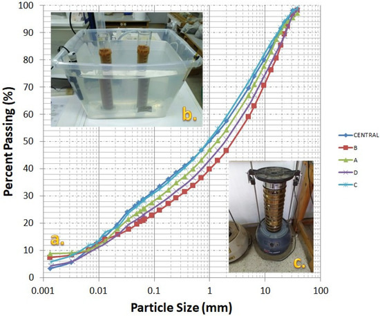
Figure 3.
(a) Particle size distribution curves for boreholes A, B, C, D and CENTRAL with a sieving technique for coarser particles (c), and the hydrometer technique for very fine particles (b).
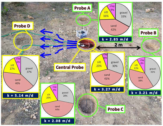
Figure 4.
The 3-D probe array developed for the second phase of the infiltration experiment and the respective grain size analysis and hydraulic conductivity of each borehole. Only the central probe and probe D recorded soil moisture variations during the first and second phases of the experiment. The blue arrows indicate the infiltrating waterfront direction based on the results of the second phase.

Table 1.
The textural class and grain size analysis of each borehole, as a weight percentage of the total sample’s dry weight, after the disposal of organic matter. The coefficient of uniformity (Cu), the coefficient of curvature (Cc) and hydraulic conductivity (k) were also extracted from the particle size distribution curve.
The most fundamental takeaways from the particle size distribution curves are summarized in Table 1. The grain size analysis showed that the five soil samples comprised mostly gravel and sand at a percentage that consistently exceeded 70%. The clay fraction was a single-digit number in all cases, while the silt percentage was relatively high, between 13 and 23%. The aggregate amount of silt and clay almost reached 30% in boreholes C and Central. These percentages of fine materials suggested high hydraulic conductivity values, which were validated by the values estimated from the curves utilizing the Hazen method. Hazen (1911) [113] proposed an empirical equation (Equation (1)) that calculates the hydraulic conductivity from a particle size distribution curve, where k is the hydraulic conductivity and D10 is the effective grain size. Borehole D presented the highest hydraulic conductivity value and borehole C presented the lowest.
The coefficient of uniformity (Cu) and the coefficient of curvature (Cc) are other indicators of soil quality. If Cu is greater than six and Cc lies between one and three, the soil is considered well-graded, as the soil in boreholes B and D, while the soil from boreholes A, C and Central is considered gap-graded. These facts can also be deduced from Figure 3, where curves B and D are smoother than curves Central, A and C.
All samples were classified as sandy loam on the soil textural triangle (Figure 5), with respect to their percentage of sand, silt and clay, according to the soil taxonomy by the USDA. However, because of the large percentage of gravel, the textural class of samples A, C and Central was better defined as stony sandy loam, while that of samples B and D was defined as very stony sandy loam, according to the USDA. The stony nature of the samples and the high percentages of gravel and sand are the result of filling and construction works.
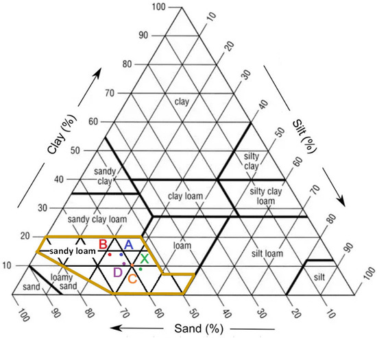
Figure 5.
The textural class of borehole samples A, B, C, D and Central (X) is sandy loam, as shown on the soil textural triangle by the USDA.
2.3. Inverse Modeling for the Estimation of the Soil Moisture Profile
The most common TDR probes use the measurement of the average water content along their length, which is useful for applications such as hydrological balances where the total soil water depth has to be estimated [54]. However, the measurement of the vertical water content profile along the probe is quite useful in applications, such as irrigation planning, crop management, aquifer recharge, runoff/flood forecasting and solute transport handling [114]. A soil moisture profile can be realized in three ways. First, by installing several vertical TDR probes of varying lengths or horizontal probes at different depths [52]. Second, by installing a custom probe with special discontinuities that produces reflections and acts as multiple horizontal probes [25,115,116,117,118,119,120,121,122,123]. Third, by using a numerical inversion model for the reconstruction of the soil moisture profile along the probe. The first two methods are based on the average soil moisture along the probe, while the third one processes TDR data extracted from the reflections along the rods. Numerous TDR waveform inversion techniques have been developed over the years for the estimation of soil moisture profiles [19,46,47,52,124,125,126], but they are not error-free. Common issues are the validity of the wave propagation model, the non-uniqueness of the inverse solution and accuracy of TDR measurements, since they are influenced by soil salinity, temperature, moisture content and cable properties [52].
In this work, the one-dimensional model of Todoroff and Lan Sun Luk (2000) [19] was selected for the estimation of soil moisture profiles from TDR signal traces. It is a numerical model that estimates soil moisture profiles along probes from the waveforms measured [19]. The first stage of the model includes the direct computation of simulated signal traces from the dielectric permittivity distribution of the surrounding soil where the pulse propagates. The second stage is basically the first stage in reverse order, hence the name inverse model. The moisture content distribution along the transmission lines is estimated from the reflected traces of the electromagnetic pulse. The model regards the propagation medium as heterogeneous, and the transmission line is divided into infinitesimally small sections of different lengths, dz, but identical transit time, where each one is considered as homogeneous, characterized by an inductance, Ldz, a resistance, Rdz, a capacitance, Cdz and a shunt value, Gdz. For real-time estimations, the authors assumed that the propagation medium is lossless, i.e., the conductance (G) and the resistance (R) are non-existent and there is no electrical resistance or conduction between the conductors [19].
Each infinitesimal segment of the transmission line is traversed by two voltage waves, traveling in the positive (U+) and in the reverse (U−) direction, called upgoing or transmitted and downgoing or reflected wave, respectively. The propagation of the pulse in the soil is regarded as a succession of elementary propagation processes, each producing a transmitted and a reflected wave at the junction between these segments. Each junction is characterized by a reflection coefficient (ρ) and a transmission coefficient (1 + ρ) for the upgoing wave (U+) and a reflection coefficient (−ρ) and a transmission coefficient (1 − ρ) for the downgoing wave (U−). The reflection coefficient is the ratio of the reflected and transmitted wave and is affected by the impedance difference between two consecutive segments. Equations (2) and (3) are used for the calculation of transmitted and reflected wave echoes at each junction. The electromagnetic pulse produces a sequence of echoes due to the transmission and reflection processes at the junctions between the segments, and the impulse response of the system at the start is generated [6].
where and are upgoing wave echoes and and are downgoing echoes, while and are reflection coefficients and and are transmission coefficients at the junction between segment and [19]. For the complete guide of impulse response, reflection coefficient, impedance and dielectric constant computation, from the initial signal traces, the reader should refer to [19].
The apparent relative dielectric constant profiles estimated with this inverse modeling approach were finally converted into water content profiles by applying the universal calibration equation by [17] (Equation (4)), where is the volumetric water content () and is the apparent relative permittivity. This equation was selected because it is easy to apply and is valid for the soil of the experimental site. It has been found to give erroneous measurements for low-density, highly organic, heavy clay and artificial soils, such as glass beads, and soils with a high content of greatly dielectric minerals [20,127,128,129,130,131,132,133]. In addition, this equation provides questionable results for volumetric water contents below 0.05 and over 0.5 and in rock samples, where it overestimates the water content because of low porosity [54,134,135]. For these types of soils, site-specific calibration is almost a necessity. Topp’s equation should be restricted to mineral soils with low quantities of bound water, like sands and loams [23]; since these types of soils were used to establish this calibration equation, it is valid for 3 < < 40.
Although this model presents some weaknesses, it can provide valid results under certain conditions. As [19] state ‘although this model does not take into account either wave relaxation phenomena or the electrical conductivity of the medium,
very satisfactory results were obtained by filtering the final reflection coefficient profile. Filtering of the reflection coefficients had to be incorporated to compensate for the high sensitivity to noise of the iterative computation and the simplicity of the propagation hypothesis. The inverted profiles are very close to the direct measurements, validating this model for measurements in low loss soils’.
3. Results
3.1. TDR Measurements
TDR was selected as a standard monitoring method for providing accurate, continuous and in situ soil moisture profiles in the vadose zone. The purpose of this work was to expand the spot use of TDR to a more spatial approach, study the response of custom spatial probes during the infiltration experiment and evaluate the results in relation to the coarser subsurface images obtained with ERT and GPR.
During the first phase of the experiment, a single probe, installed in the center of the grid, was used to monitor the vertical water movement below the point from where the water infiltrated the soil. In the second phase, a 3-D array with four more probes was developed (Figure 12) to provide a more spatial image of soil moisture distribution in the unsaturated zone.
The spatial probe technique was selected to measure the soil moisture profile along the probe and not at discrete depths. The probes used in this work are of identical design. They are made of three flat enameled copper wires (6.3 mm × 1.0 mm), serving as waveguides, glued parallel to each other, with 1 cm spacing, onto a standard HDPE tube with a diameter of 6 cm (Figure 6). The length of both the waveguides and the tube is 1 m. Copper was selected because of its low cost and great electrical properties. It has one of the highest levels of electrical conductivity among all metals and is a great transmission line for the propagation of high-frequency electromagnetic pulses emitted by a TDR instrument. A 50-ohm RG-58 C/U MIL coaxial cable with a length of three meters and a 50 Ω BNC male connector was used for the connection between the probes and the instrument. The central signal pin of the coaxial cable was soldered to the central copper wire, while the ground (outer sheath) of the cable was split and soldered to the outer two copper wires [18]. An impedance-matching transformer (balun) was not necessary since the three-rod probe emulates the coaxial cable [16,21]. Constructing custom probes lowers costs and provides designs that better fit specific applications.
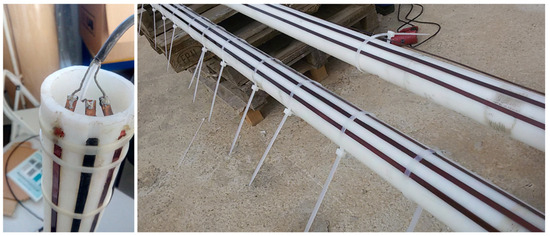
Figure 6.
The custom TDR probes with three flat enameled copper wires.
These custom probes are durable and destined for longer or even permanent deployment in the ground without losing performance. However, extra precaution is needed during their installation into predrilled boreholes. Poor installation and soil disturbance are the largest sources of error in estimated volumetric water content. If installation is poor, the measurements will be inconsistent no matter how good the calibration and the instruments are. Errors can result from a deviation in the parallel array of the rods and the creation of air gaps that greatly affect the estimated water content because of the very low dielectric permittivity of air. The electromagnetic field is much denser near the waveguides where air gaps typically occur, and the sensor is more sensitive there. These few cm next to the probe have the most influence on the reading and, as a result, when a gap is formed, the sensor measures air instead of soil. Also, air gaps reduce the penetration of the electromagnetic field into the surrounding soil. These can lead to an underestimation of the volumetric water content and even to negative measurements. The goal of installation is to produce optimal contact between the soil and the probe. The borehole should be straight and smoothly sliced and have the correct diameter to obtain not only error-free measurements but also measurements representative of the original soil. Installation in disturbed soil will produce unrepresentative measurements since the soil properties have been altered. In order to measure correctly, all parts of the waveguides need to be in direct contact with undisturbed soil. If any part of the sensor is not touching the soil, that part may measure air or pure water, which will alter the soil moisture data. The errors from poor installation in the literature have been cited at 10%, 15% or even more than 20%. Sometimes, air gaps can be created even if the installation is appropriate because of natural causes, such as voids created by insects, rodents and plant roots, or because the soil, especially clay, has dried and fissures have developed.
In this work, all probes were vertically installed into pre-drilled boreholes (A, B, C, D, Central, Figure 12) with their bottom at a depth of 1.2 m from the surface and their top at 0.2 m so that they were the same height as the bottom of the double-ring setup. The gap between the probes (diameter of 6 cm) and the borehole walls (diameter of 7.5 cm) was quite small. Nevertheless, this gap was backfilled with the same material originating from each borehole. The waveguide side of the probes was pushed against one side of the borehole, and the gap at the back was filled with the original material in reverse order when extracted to avoid mixing the soil horizons. That material was sieved and mixed with water in order to remove large stones and gravels and achieve the best contact possible between the probe and the undisturbed borehole walls. Nevertheless, because of the presence of large stones in the undisturbed soil, backfilling was necessary even on the waveguide side of the probes to minimize air gaps.
After the installation, a few months passed before the execution of the first phase of the experiment, allowing the backfilled soil to consolidate in a natural way and possible air gaps to close up with the natural settlement of the loosened soil [27]. However, it is not easy to say to what extent this may occur or how much time it needs since it depends on precipitation, soil type and density. Be that as it may, we managed to maintain the nature of the original soil and hopefully achieved an average bulk density that was not very different from that of the original medium, leading to soil moisture estimations as representative as possible. When backfilling, compacting the soil too tightly or repacking it too loosely generates preferential flow and causes the water to move through different pathways and at different speeds.
The instrument used was TDR100 by Campbell Scientific Inc. (Manufacturer: Campbell Scientific Ltd., Loughborough, UK). This pulse generator can accurately determine soil volumetric water content. TDR100 generates a short-rise time electromagnetic pulse, which is applied via a coaxial cable to the probe and samples and digitizes the resulting reflection waveform for analysis or storage (TDR100 instruction manual, Campbell Scientific Inc.). SDMX50, an eight-channel, 50-ohm coaxial multiplexer by Campbell Scientific Inc., was also used for the continuous and automated reflection waveform measurements of up to eight different probes. During the first phase, the multiplexer was not necessary since only the central probe was attached directly to TDR100. Lastly, the CR800 data logger by Campbell Scientific Inc. was used for the automated storage of the waveforms (Figure 1c). For the configuration and troubleshooting of the aforementioned TDR100-based system, such as the definition of the time interval between measurements and the configuration of the program used by the datalogger for automated waveform measurements, PC-TDR software (version 3.0) by Campbell Scientific was used.
During the first phase, the water infiltrated the soil for more than four hours at a constant flow of about 1 L/min after the sorptivity phase. TDR measurements were conducted using the central probe, with a time interval of one minute. Measurements were also conducted before and after the experiment to image the initial soil moisture profile and post-infiltration soil response, respectively.
The output of a TDR measurement is a reflection coefficient versus time graph. The reflection coefficient is the amplitude of the reflected signal to the amplitude of the transmitted signal. Time represents the two-way propagation time of the electromagnetic signal along the transmission line. Figure 7 presents a waveform measured at the central probe comprising the successive reflections of the incident signal and their respective recording time. From this waveform, using the part between the start and the end of the probe, the apparent relative dielectric constant profile of the surrounding soil along the probe can be estimated utilizing the inverse model by [19]. The part before the sensor starts represents the propagation of the pulse inside the coaxial cable, while the one after the end of the probe is mostly used to derive information about the electrical conductivity of the medium, but this is not something that this work dealt with. The estimated dielectric constant profile was finally converted into a volumetric soil moisture profile (Figure 7b) using the universal empirical equation (Equation (4)) by [17]. This algorithm was used to estimate the moisture profiles for all probes during the first and second phases of the experiment.
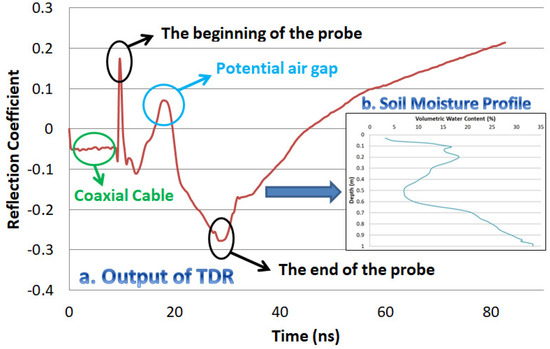
Figure 7.
(a) An output TDR waveform of the central probe. Only the part between the beginning and the end of the probe is used to estimate the apparent relative dielectric permittivity profile, using Todoroff and Lan Sun Luk’s inversion model. (b) The soil moisture profile calculated using the universal equation by Topp et al. (1980) [17].
The setup comprising the custom probes, the instruments, the inversion algorithm and the calibration equation, was tested several times over the last few years, both in the lab and the field, with different kinds of soils. The deviation between the volumetric water content estimated from TDR measurements and that measured from the respective soil samples using the gravimetric method and the bulk density of the samples was no more than 3–4% in most cases. Based on these results and because of the fact that the whole soil sample extracted from each borehole had to be used for grain size analysis, the bulk density and the gravimetric water content were not measured in this study, and a comparison between the estimated and measured VWC was not conducted.
Figure 8 presents selected volumetric water content profiles from the central probe, from the start to the end of infiltration, estimated using the inversion model by Todoroff and Lan Sun Luk (2000) [19] and the calibration equation by Topp et al. (1980) [17]. Every depth presented on the VWC graphs is in reality 0.2 m deeper since the zero value corresponds to the top part of each probe that lies 0.2 m below the ground surface. For better visual representation and convenience, each profile depth ranges between 0 m and 1 m.
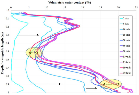
Figure 8.
The VWC profiles estimated from TDR measurements from the central probe conducted during the first phase of the experiment. The arrows pointing towards the right indicate a soil moisture increase, while the yellow areas and the dashed arrows pointing left indicate a soil moisture decrease. The measurement times are presented in the legend.
The first line (0 min) presents the moisture profile of the soil surrounding the probe in dry conditions before infiltration. At a depth between 0.1–0.3 m and 0.9–1.0 m, the soil moisture is around 3–4%, while at the surface (the bottom of the double-ring setup) and between 0.4 and 0.85 m, it is close to zero, which is definitely not a natural state of any soil and possibly indicates the presence of air gaps formed around the waveguides. Very small VWC values in dry conditions are probably not a big deal and are presumably due to the use of a generic calibration equation like the one by [17], which produces small errors at the low end. Soil-specific calibration increases accuracy to ±2–3% and eliminates such errors.
Five minutes after the start of the water supply, a moisture value between 4 and 11% can be seen throughout the whole length of the probe (green line), which is probably evidence of preferential flow induced by the probe itself that generates a vertical pathway for the downward flow of water. A body of water flows against the probe, and after just five minutes, it already reaches the bottom end of the probe. In the next 10 min, the soil moisture keeps increasing rapidly. After that time and until the cessation of the water supply after 250 min, the moisture profiles present little variations. This probably means that the soil surrounding the probe reached a near-saturated state. In this state, the moisture between 0.1 and 0.3 m ranges between 14 and 19%, while at deeper horizons between 0.7 m and 1.0 m, exceeds 20% and almost reaches 35% at a certain time. Between 150 and 250 min, the moisture profiles present a small decline. After 150 min, the soil probably reached a near-saturation state, and from that point onwards, every decrease in water flow (Table 2) results in a VWC decrease. This water flow decrease probably indicates changes in the saturation of the parts of the soil that affect the measurements. If the flow decreases, the water infiltrates deeper and the above area changes from a saturated to a less saturated state, and as a result, TDR senses less water and the volumetric water content decreases.
Table 2.
The water flow from the tank during the experiment.
The most noticeable observation in all profiles is the abrupt moisture decrease between 0.2 and 0.6 m. This decrease, along with the almost zero initial moisture content, in all probability indicates the presence of air gaps at these depths that heavily underestimate the water content. Some soils, like clays, can also cause cracks to form around the sensor. As mentioned, the electromagnetic field generated is more sensitive right next to the waveguides and, because the sensing volume of a probe is just a few cm, the sensor is greatly affected by the air layer and much less by the soil layer beyond the air gaps. This moisture decrease could also mean the existence of a compacted and less permeable horizon at that depth, maybe due to drilling, which impedes the water from flowing in the soil, and the only flow against the probe happens because of adhesive and cohesive forces. This decrease is not obvious in ERT tomograms (Figure 12), which is rather reasonable because of the coarser resolution of ERT. TDR senses differences that ERT cannot because of its very small sensing volume. Also, more water is accumulated near the bottom end of the probe where the moisture almost reaches 35%, which indicates a more permeable layer in that area, in contrast to the zone between 0.1 and 0.2 m, where the moisture is less than 20%.
After the cessation of the water supply, the instruments were left on and buried in the ground to monitor the water holding capacity of the soil and how the moisture settled during a period of selected VWC profiles right after the water supply stopped and for several hours later, as well as on selected days afterward. The first noticeable decrease in soil moisture is observed 10 min after the water supply stopped (green line). During this 10 min period, the infiltration process remains almost the same since the double-ring setup was half-filled with water that needed to infiltrate the ground. During the next five minutes, the moisture decreases quite rapidly from 17% to 12% at 0.2 m and from 20% to 10% at 0.8 m. This fact indicates once again a very permeable medium with low water holding capacity. When the supply of water stops, the soil cannot retain much water, which infiltrates deeper because of gravity. After 45 min, the moisture keeps decreasing but at a lower rate since most of the water already left the soil surrounding the probe. The changes are minor and are mostly witnessed at 0.2 m and below 0.8 m. At 0.2 m, the moisture drops from almost 19% at the cessation of water supply to almost 7% after more than three hours. The alterations can be better understood starting from the bottom of the graph, where the profile lines are more discernable.
Selected measurements are presented for one to seven days after infiltration. The soil moisture keeps decreasing, mainly in the upper and lower parts of the sensor. At 0.2 m, the moisture drops from around 6% after one day to less than 5% after seven days. However, after three days, there is an abrupt increase to 9% (blue circle) due to water infiltrating the soil after a light rainfall event in the afternoon on that day. A slight soil moisture increase due to rainfall can also be noted below 0.8 m, which is once again a clear indicator of the high infiltration velocity resulting from the preferential flow produced by the probe itself. The profiles between four and seven days are almost identical below 0.3 m, which suggests that this part of the soil reached field capacity. All the gravity-drained water leaves the system, and the remaining water is held by suction in mesopores and micropores. In the middle part, between 0.4 and 0.8 m, the moisture is almost zero, possibly because of air gaps and a potential impermeable layer; thus, less water is concentrated into the sensing volume of the sensor, and lower moisture values are estimated there. Lastly, all soil moisture profiles present the same pattern of abrupt decrease between 0.2 and 0.7 m, similar to the ones during infiltration, which shows that serious air gaps are still present between the probe and the soil at those depths. Figure 9, just like Figure 8, shows greater moisture near the bottom part of the probe. The water drains quite fast since after just a few hours, the available water has infiltrated deeper because of gravity and the soil has nearly reached field capacity. The greater moisture percentage near the bottom end and the fast drainage indicate the presence of a more permeable layer below 0.7 m, seemingly with more coarse material and less clay.
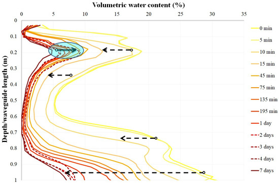
Figure 9.
Selected VWC profiles of the central probe after infiltration. The arrows pointing towards the left indicate the general trend in the soil moisture decrease, while the blue circle and the arrow pointing right present a VWC increase due to a rainfall event.
During the experiment, the flow from the tank, indicating the flow with which the water was infiltrating the soil in the inner ring, was measured with the use of a flowmeter, as shown in Table 2. In the beginning, where the soil is unsaturated and sorptivity is in effect, the flow is 2.2 L/min. After three hours, the soil is nearly saturated, and the flow is constant at 1 L/min.
As seen in Table 1, the central borehole comprises 71% coarse material, which means that the water holding capacity of the soil is not that great. It drains fast, and it is saturated fast, which is more obvious near the bottom part of the probe where the water presence is greater.
In the second phase of the experiment, four probes (A, B, C, D), identical to the central one, were installed two meters apart from the center of the plot in a cruciform array (Figure 12) to investigate the capacity of TDR to monitor hydrological processes in a more spatial manner and provide more information about the behavior of the infiltrating water. This phase was conducted under the same conditions as the first phase. The water supply lasted for four hours, and a total volume of approximately 500 L infiltrated the soil. TDR measurements were automatically recorded and stored in the datalogger during the experiment, with a time interval of one minute.
Figure 10 presents the reflectograms of the four newly installed probes during the second phase. Each graph presents the reflectograms for each probe from the beginning to several hours after the end of infiltration, except for probe D because of an unexpected malfunction in the respective channel of the multiplexer that led to distorted measurements after 4.5 h. During infiltration and several hours after the end of it, probes A, B and C showed no sign of water detection since all reflectograms were identical. No water reached these probes, either by gravity or capillarity. However, this was not the case with probe D. Although during the infiltration there was no sign of water presence, a reflectogram deviation appeared the exact moment when the water supply stopped after four hours (Figure 10). Between 240 and 260 min, the reflection coefficient kept decreasing, which validates the arrival of infiltrating water at probe D. The lower the reflection coefficient, the more conductive the medium.
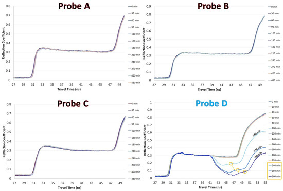
Figure 10.
The output reflectograms of the four newly installed probes during the second phase of the experiment. Only probe D presents reflection coefficient variations after 240 min (yellow circles and yellow box), which indicate the arrival of the infiltrating water at this probe.
Figure 11 presents the soil moisture profiles for probe D, from the infiltration start to 20 min after the cessation of the water supply. These profiles were estimated from the reflectograms in Figure 10, applying the inversion model by Todoroff and Lan Sun Luk (2000) [19] and the calibration equation by Topp et al. (1980) [17]. During infiltration, there is no VWC change. The initial moisture of the medium surrounding probe D ranges between 6 and 10% and increases with depth, probably because the water from the first phase infiltrated deeper because of gravity, while near the surface, the soil lost some moisture because of evapotranspiration and capillarity. These values are greater than those of the central probe before infiltration, probably because the water of the first phase moved in this direction as well. The soil retains some moisture; therefore, more pores are filled with water and the moisture estimated is higher. After 240 min, however, the infiltrating water reaches the lower part of the probe below 0.6 m. Between 240 and 260 min, more water accumulates around the lower part and the VWC keeps increasing, while the part above 0.6 m remains unaffected. Presumably, if probe D’s measurements were not corrupted after 260 min, water content variations would be present around the upper parts as well since there seems to be a permeable soil layer in this direction with high hydraulic conductivity, as indicated in Table 1. As a result, the infiltrating water follows this route and enters the sensing volume of the probe, generating higher moisture estimations.
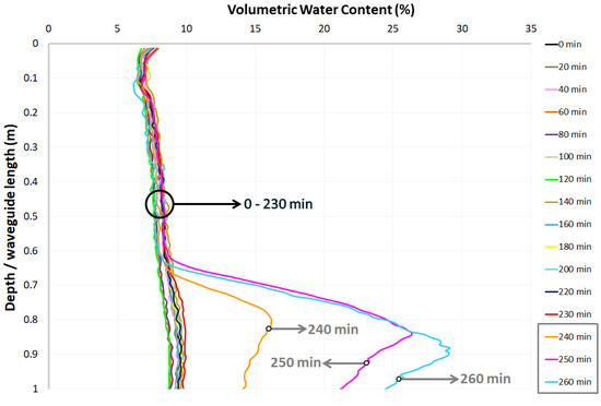
Figure 11.
The soil moisture profiles of probe D during the second phase of the infiltration experiment. After four hours, the water reaches the lower part of the probe and for the next 20 min, the water content keeps increasing.
The average velocity of the lateral movement of the water, in the direction from the plot center to the lower part of the probe, was calculated at around 0.56 m/h using Equation (5).
3.2. ERT Measurements
The purpose of these measurements was to investigate the capacity and constraints of electrical resistivity tomography (ERT) to capture the resistivity allocation in the unsaturated zone of an urban area disturbed by anthropogenic fills during a forced infiltration experiment and complement the information provided by TDR during the first two phases with a much more spatial approach. The electrical resistivity of the soil is affected by various soil properties such as soil moisture, texture, porosity, pore water resistivity and soil temperature [136]. The alterations in the resistivity affected by the dissemination of the water plume are presented as a function of time. The ERT results were also assessed for their level of agreement with the geological and hydrological data of the area and with the TDR and GPR results.
ERT uses multiple four-electrode measurements to image the soil resistivity distribution in 2-D or 3-D mode. An electrical current (I[A]) is injected into the soil by two current electrodes, and the difference in the resulting voltage (U[V]) is measured by two potential electrodes using several combinations among these electrodes along a transect or grid [66,97,137]. By shifting the electrodes further apart, deeper and bigger lateral coverage of the subsurface can be achieved. This potential difference and the geometrical arrangement of the electrodes provide an image, known as a tomogram, of the resistivity model of the subsurface, considered homogeneous half-space, after geophysical inversion processing. Since the inversion process is ill-posed, the estimated model is non-unique and indicates a smoothed representation of the true resistivity distribution [66].
The measurements were conducted with a SYSCAL IRIS PRO instrument by Iris Instruments, with 10 parallel channels, using 72 electrodes, in a 7 m × 8 m grid. The design of the grid was based on the results of the second phase in order to validate the flow imaged by TDR. The pole–dipole array was selected for a better lateral and vertical resolution of the subsurface. The obtained data were processed with Res3Dinv. A Leica Differential GPS series 1200 system was used to position the infinite electrode.
The third phase of the experiment lasted for more than four hours, and a total of ten measurements were conducted. Selected tomograms of these measurements are presented in Figure 12. Each measurement took about 24 min to complete, and the respective tomogram imaged the subsurface at a depth of up to two meters. The first measurement (0 min) was conducted before infiltration, in dry conditions, to obtain a glimpse of the subsurface in its natural state and a reference image on which the interpretation of the subsequent images was based. The contrast between the dry and wet stages of the soil was used to distinguish the static resistivity distribution from the variations produced by the infiltrating waterfront [9]. At 0 min, with no water infiltrating the soil, the subsurface is characterized by non-uniformity. The reddish left side zone presents lower resistivity values (around 120–130 ohm.m) than the yellow right-hand side (greater than 200 ohm.m), which might be an indicator of the presence of more fine-grained, loose and not-so-well-compacted material (silts and clays) that generally is less resistive because of its water holding capacity due to matric forces. The percentage of coarse material is high (Table 1), while the interstices are probably filled with fine-grain material. However, as it can be seen in Table 1 and Figure 3, borehole D, which lies in the reddish area, indeed contains fine-grained material but presents the second lowest sum of silt and clay in relation to all the samples and predictably has the highest hydraulic conductivity values. Furthermore, the sample of borehole D is characterized as well-graded. In the same way, the more resistive yellow area implies coarser and more cohesive materials, which is not entirely true based on Table 1 because of the presence of fine-grained material at a percentage of more than 20% in all directions. Gravel presents the greatest variation, up to 13%, between boreholes C and B, while the deviation between sand and clay is 6% and 3%, respectively. Considering this, a possible explanation for the non-uniformity of the underground could be a difference in compaction between the different zones of the subsurface. Also, a few weeks before the first phase of the experiment, the double-ring infiltration test took place. The higher conductivity areas could be the result of the moisture retained by the fine-grain material in the soil because of matric suction that was neither evaporated nor infiltrated deeper. The yellow, brown and green areas potentially represent coarse-grained and coherent soil unaffected by the infiltrating water of the double-ring test. Unfortunately, a meticulous grain size analysis every 10 or 20 cm was not possible because of the nature of the soil, and we can only speculate about the soil profile at each depth.
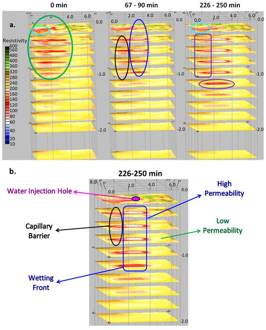
Figure 12.
(a) Selected 3-D ERT tomograms of resistivity distribution changes during the point source infiltration experiment depicting the vertical (dark blue circle) and lateral (purple rectangle) dissemination of the water, as well as the resistivity distribution before infiltration (0 min) and the initial less resistive area of the unsaturated zone (green circle). The black circle suggests possible channels from where the waterfront may flow out of the image plane. Light blue circles indicate the change in resistivity before (0 min) and after infiltration (250 min) and the dissemination of water due to capillary forces. Times indicate the timeframe of each measurement from the start of infiltration. (b) An ERT tomogram interpretation with areas of high permeability (red and white areas) where the water infiltrates and areas of low permeability (yellow and brown areas) where flow is almost non-existent. The capillary pressure is the main cause of the lateral dissemination of water (black circle).
We can see the vertical movement of the infiltrating waterfront (blue circle) in the center of the grid 67–90 min after the infiltration started, below the double-ring setup, with very low resistivity values, which reached a depth of 1 m. On the other hand, there does not seem to be important lateral movement of the waterfront just yet, which is an indicator of preferential flow around the central probe. Only after the saturation of this part, the water will start moving laterally.
In general, resistivity decreases as moisture increases. The tomograms show changes in resistivity, not in moisture content. Soil water content and resistivity are not connected in a linear way since resistivity is more sensitive to water content changes at lower saturations; their relationship is also dependent on the type of soil [9]. An ERT tomogram shows the permeable formation that bears the water and not the water itself. A permeable formation has high electrical resistivity because of a high percentage of coarse material, and this is where the flow of the water takes place. A less permeable soil, like clay, is more conductive and impedes water flow through its mass.
During the last measurement (226–250 min), at the end of which the water inflow was shut off, the lateral dissemination of the water is quite visible (purple rectangle), and more water infiltrated deeper. Between 1.2 and 1.6 m, the reddish areas of low resistivities increased. Nevertheless, there is no visible infiltration below 1.6 m since there is no resistivity change. Some water might have infiltrated that depth, but it is not discernible in the tomogram because the sensitivity of the inversion model is lower in the deeper layers than in the surface layers. This could also be an indication of a coarse-grained layer that cannot hold much water, and a resistivity change is not visible. The lateral spread of the waterfront is bigger at 0.4 m, and it becomes smaller with increasing depth. This effect could be attributed to a ‘capillary barrier’ [9]. If a fine grain material, like clay, lies on top of a coarser soil, like sand, water will start to infiltrate the coarser material only after the fine soil is saturated. Fine-grain soil has smaller pores and greater capillary pressure and will not let the water leave until it is saturated. Once water enters the coarse layer, it moves fast towards the next bottom layer.
Gravitational and capillary (adhesion and cohesion) forces act simultaneously and are the two primary forces that govern water movement through soil. When water is first applied to dry soils, it moves outward almost as far as it moves downward since capillary action happens in unsaturated soils. Initially, the pores in the soil are unsaturated. Water flows mainly through the smaller pores because of strong adhesive and cohesive forces that can move water in any direction. Eventually, the pores are filled to near saturation because the water is applied at a faster rate than it can be moved by capillary forces. Since the largest pores are now filled, they conduct water faster, and because capillary forces are not as great in larger pores, gravity becomes dominant, and the water moves downwards. In this experiment, the preferential flow that is the result of the presence of the central probe impedes the matric suction and the lateral movement of the infiltrating water until the surrounding soil is nearly saturated. The vertical and lateral movement of the waterfront seems to follow a constant pace, without sudden outbursts of acceleration or deceleration.
The highest change in resistivity, before and after infiltration, is around 60 ohm.m (from around 120 ohm.m of the reddish area to 60 ohm.m of the white area). To ensure a better resolution and a more visible signature of soil moisture changes, high conductivity water (around 990 μS/cm) was used, originated from boreholes inside campus. This conductivity would not lead to unusable TDR and GPR results.
The direction of the plume shows a clear preferential flow towards the left-side zone where probe D is situated. This agrees perfectly with the TDR results from the second phase and with the grain size analysis (Table 1), where the borehole D sample presents the highest hydraulic conductivity and the second highest aggregate percentage of coarse-grain materials (sand and gravel). Water penetrates faster and deeper in coarser soils with open macropores, like sand and gravel, than it does in material with micropores, like silt and clay. Coarser soils have larger pores that absorb water faster and hold less water per unit of depth. Nonetheless, the grain size differences among all samples are not that notable, and the plume, despite some logical dissimilarities in the propagation velocity, should be disseminated radially around the central probe. However, there is no sign of water disseminating towards the other directions, even after four hours of constant infiltration, which probably indicates a difference in the homogeneity and the compaction of the soil and the presence of a layer with less pore space around the probe that impedes the water movement and generates strong preferential flow towards borehole D. The soil in this direction seems to be more homogeneous, permeable and less compacted, as indicated by the high hydraulic conductivity of borehole D sample. The compaction differences can also be seen in the double-ring and single-ring test results (Figure 2). The integral calculation with the single-ring equation for a period of 250 min gives a total volume of 683 L, while with the double-ring equation, a volume of 294 L is obtained. While the different locations of the two setups and the presence of the probe in the center of the double ring play a major role in the differences in the infiltration volumes, such deviation could be justified by serious compaction differences. Furthermore, a possible flow towards the other directions may happen via narrow channels that are barely resolvable, and a portion of the water may flow out of the image plane from channels such as the ones suggested within the black circle in Figure 12a.
The central probe is another factor of preferential flow. The infiltrating water flows against the probe and finds a way out only in the left direction. In the other directions, a restraining and highly compacted layer could hinder that flow. All forms of preferential flow increase the percolation rate, providing shortcut paths through cracks and pores and allow deeper penetration of water under the force of gravity. Fast and far-reaching preferential flow is an undeniable part of groundwater hydrology.
That flow alters the resistivity of the soil, depicted as white area in the tomograms, with resistivities around 50–60 ohm.m that become as low as 40 ohm.m (light blue areas). The average infiltration velocity was calculated with Equation (5) to be around 0.4 m/h, or 6.66 mm/min, mapping the movement of the same isoelectrical values and measuring the distance that the waterfront covered. The central borehole presents the highest fine-grain percentage, with an aggregate of almost 30% silt and clay. This means that the water movement is slow because of strong capillary forces. The water does not percolate deeper until the layer above becomes saturated.
Regarding lateral dissemination, the waterfront spread more than 3 m at a depth of 0.4 m and more than 2 m at a depth of up to 1 m, which implies a hydraulic conductivity between 0.5 and 0.7 m/h. Therefore, the waterfront moved both vertically and laterally, because of gravitational and capillary forces, at approximately the same speed.
The point of entry of the water into the ground at 0.2 m of depth and the change in resistivity at the same depth (light blue circles), indicate that the flow there occurs because of capillary suction that forces the water to disseminate laterally. This fact likely indicates a large percentage of fine-grain material in the upper soil horizons and highlights the capability of ERT in imaging capillary outcomes.
Heterogeneity and compaction differences probably push the preferential flow of the water in one direction. The hydrological properties and the plume formed during the experiment are not those of a uniform porous medium. In many cases, they are inconsistent with the grain size analysis and pose a challenge for the accurate delineation of the hydrogeological processes of the vadose zone. However, ERT provided qualitative time-lapse images of the size, shape and behavior of the plume in a hydrologically complex environment. This could be of great assistance for the further investigation of site hydrology when combined with other geophysical methods, such as seismic methods, that could provide data about the compaction state of the soil. ERT benefitted from the high conductivity of the water and could image the capillary movement in the unsaturated zone.
ERT measurements validate the results of the second phase over the flow direction of the infiltrating water. The ERT tomograms show a clear preferential flow towards borehole D that matches perfectly with the TDR results. Therefore, the flow imaged by TDR is not incidental. There is a permeable path in the direction that the water tends to follow. The hydraulic conductivities calculated with ERT and TDR also coincide. Although these velocities are the outcome of an extreme artificial infiltration event, they show that TDR and ERT can be adequately used to estimate the velocity of liquid wastes and pollutants in the unsaturated zone and the time it takes before they reach the aquifer. There is a strong macroscopic agreement between TDR and ERT, and the discrepancies between them are probably because of the different sensing volumes of the methods.
3.3. GPR Measurements
The purpose of these measurements was to investigate the capacity and constraints of GPR to capture the movement of conductive water into the soil and provide further spatial insight into the unsaturated zone and the processes that take place there during an artificial infiltration test. GPR was selected because it can image large volumes of soil relatively fast and cost-effectively. Also, its operation is based on similar principles to TDR. Both methods are dependent on the dielectric permittivity and electrical conductivity of the soil. This makes these methods a good supplement technique for each other [138]. TDR can provide more detailed point measurements of soil properties (a few cm3 around the probes), while GPR’s resolution is coarser and appropriate for imaging larger volumes of the subsurface in the order of several m3. A drawback of GPR is that the measurements have to be conducted manually, which makes the method inappropriate for continuous monitoring, while automated data acquisition is very common in TDR measurements [28]. On the other hand, for a more spatial image of the soil properties using TDR, numerous probes have to be installed at several locations.
A typical GPR setup comprises a transmitting antenna that emits a high-frequency electromagnetic wave into the ground and a receiving antenna that measures the amplitude of the reflected wave as a function of time [139] (Figure 13). The propagation velocity of the radar waves is mostly dependent on the dielectric constant of the soil, just like TDR, which is strongly related to soil moisture [17]. Any change in the dielectric properties of the soil will result in reflecting part of the wave energy back to the surface [26]. The depth of penetration ranges between a few cm and tens of meters and depends on the center frequency of the antenna and the electrical properties of the subsurface [56,140]. A lower frequency entails deeper penetration and poorer spatial definition, while a higher frequency entails smaller penetration and higher definition. Regarding the properties of the soil, the higher the electrical conductivity of the soil, the stronger the attenuation of the signal and the shallower the depth of penetration. Non-deionized water is by nature conductive, but its conductivity can increase depending on its salt content, which strongly affects the attenuation of the signal [139]. Therefore, the presence of water in the soil heavily alters its electrical properties, and, for this reason, GPR is better suited for shallow hydrogeological investigations [82,141].
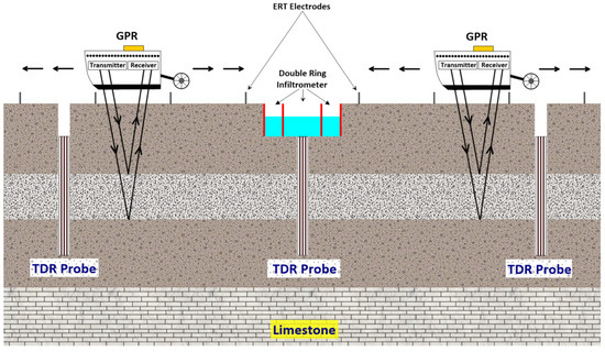
Figure 13.
Schematic drawing of the infiltration experiment with the TDR, ERT and GPR configurations.
In this study, a total of four transect lines were designed based on the water movement indicated by TDR and ERT during the second and third phases of the experiment in order to detect the same movement in 2-D and 3-D modes. Transect lines 1 and 3 had a length of 10.6 m, while lines 2 and 4 had a length of 8 m and 7 m, respectively. Transect line number 4 was expected to be of great interest since it was in the direction of the water flow recorded by TDR and ERT. Boreholes B and D were situated on both sides of the double-ring setup in the direction of transect line number 4, while boreholes A and C were situated on both sides of the double-ring setup in the direction of transect line number 2. The water inflow lasted four hours, while GPR measurements were also conducted before and after infiltration to image the initial state of the subsurface and the response of the unsaturated zone during drainage, respectively. Each round of GPR measurements comprised four measurements, one for each of the four transect lines. A total of 19 rounds were conducted. The first round was conducted before infiltration, rounds 2–15 during infiltration, and rounds 16–19 after infiltration. The GPR data was acquired with the 500 MHz MALA RAMAC shielded antenna (Manufacturer: Guideline Geo AB, SE-171 54 Solna, Stockholm, Sweden) with every 10 cm signal and processed with REFLEXW.
Figure 14 presents the amplitude envelope maps in 2-D and 3-D modes for selected rounds of measurements during and after infiltration. The first round of measurements (0 min) was conducted before the infiltration started, while the next two rounds were conducted 105 and 200 min after infiltration started. The last round of measurements at 300 min was conducted one hour after the cessation of the water inflow. Each 2-D map shows the subsurface up to 1.3 m of depth, while each 3-D map shows up to 1 m.
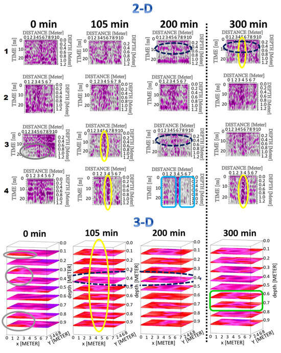
Figure 14.
Two-dimensional and three-dimensional tomograms of selected round of measurements before (0 min), during (105 and 200 min) and after infiltration (300 min). The dark blue dotted circles suggest the presence of a less permeable layer at a depth of 0.4 m, the yellow circles depict the central TDR probe, the grey circles delineate the conductive parts of the underground before infiltration and the blue and green rectangles show the absence of reflections in the direction of borehole D.
In the 2-D maps, each column represents the four different measurements of the same round, one for every transect line. The purple color indicates areas with many reflections, probably due to the presence of more coarse material, while the greyish color indicates areas with very few reflections. The importance of this study is that the infiltrating water is conductive; therefore, in the areas where the water infiltrates, there should be very few reflections due to signal attenuation. The first column represents the four transect measurements before the start of infiltration to image the initial dry state of the vadose zone and obtain a reference point for the interpretation of the resulting tomograms during the experiment. The tomograms at 0 min present many reflections in every direction, except for a part in transect line number 3 (grey circle) where there is a lack of reflections, which coincides with the ERT results regarding the presence of a more conductive horizon in dry conditions towards borehole D. That plethora of reflections may indicate that the subsurface is more homogeneous in these directions. There are fewer reflections 105 min after the start of the water inflow, i.e., in more conductive areas. In transect line numbers 3 and 4, there is a clear vertical line of reflections (yellow circles) that represent the central TDR probe. The presence of the probe generates reflections along its entire length, while around the probe, there are fewer reflections, probably indicating that the water infiltrated those areas. At 200 min, on diagonal transect lines 1 and 3, at a depth of 0.4 m, there is a fixed zone throughout the whole length of the lines with many reflections, which probably indicates a less conductive horizon (Figure 14, dark blue dotted circles). The depth of this horizon coincides with the soil moisture anomaly imaged by all TDR measurements around this depth during the first phase. The less permeable structure at 0.4 m can be seen even better in the 3-D tomograms between 105 and 200 min. On transect line 4, the contrast between the probe and the areas around the probe is quite noticeable. While the probe area is full of reflections (purple column), the areas around the probe (light blue rectangles) are very conductive, suggesting that the water infiltrated these areas. However, the area towards borehole D is almost completely free of reflections, which means that the main body of the infiltrating water follows that route. This result coincides with the TDR and ERT results and Table 1, where the grain size analysis showed that boreholes B and D have the highest percentage of gravel (41% and 37%, respectively); therefore, the soil is more permeable in this direction. In the last round of measurements (300 min), one hour after the cessation of the water inflow, it seems that the water drains quite fast since the reflections increased in all transect lines. A lot of water drains because of gravity, but the general trend is the same as during infiltration. Transect lines 1 and 2 show many reflections, while more water seems to be retained in the direction of transect lines 3 and 4, where less signal is reflected back (more grey areas), suggesting less permeable and more fine-grain material in lines 3 and 4, in contrast to the ERT results that show water movement towards borehole D only. The central probe (yellow circles) and the less conductive layer at 0.4 m (dark blue dotted circle) are visible in this round as well. In general, transect lines 3 and 4 during and after infiltration present fewer reflections, which validates TDR and ERT regarding the water movement in this direction.
For GPR data, the processing was carried out with REFLEXW for every 2-D profile as follows:
- Subtract mean (dewow);
- Correct max. phase;
- Move start-time;
- Manual gain;
- Bandpassbutterworth filter (200–600 MHz);
- Background removal;
- Spectral whitening (200–600 MHz);
- Deconvolution (0, 26, 2, 0.5);
- fk migration (Stolt) (V: 0.1 m/ns);
- Envelope.
Then, the 2-D profiles together created the 3-D GPR amplitude signal distribution.
The bottom maps in Figure 14 present the same results in 3-D. Each 3-D tomogram is the sum of the four respective 2-D tomograms. In this way, a spatial depiction of the water flow is possible at each depth. The purple and violet colors represent areas with many reflections, while the reddish areas indicate conductive areas with signal losses due to wave attenuation. In the 105 and 200 min 3-D tomograms, the layers above and below the resistive layer at 0.4 m are very conductive, which probably means that a lot of water infiltrated the soil and heavily attenuated the signal. Especially in the bottom layers, the red areas are even more dominant, which agrees with TDR that a lot of water accumulates near the bottom end of the probe. During the drainage stage, more water seems to be retained at a depth of 0.6 and 0.7 m, which attenuates the signal and produces fewer reflections (green rectangle).
The most notable GPR results are the clear depiction of the central TDR probe and the fact that the soil is affected more by the conductive infiltrated water in the direction of transect line 4. Although ERT and TDR depict the water flow towards borehole D only, all three techniques suggest that the main flow occurs in this direction. In several cases, GPR also depicted the presence of a consistent layer of reflections at a depth of 0.4 m, which validates the VWC profiles over the presence of a less permeable structure. In general, the conductive water (around 990 μS/cm) is assumed to have affected the performance of GPR more than that of ERT. Nevertheless, GPR validated some of the concepts imaged by ERT and TDR.
4. Discussion and Conclusions
Vadose zone processes play a crucial role in water resource management and environmental protection. Measuring, monitoring and predicting water storage, water fluxes and solute transport can lead to a better management and protection of underlying aquifers and ameliorate risk assessment and treatment planning of contaminated areas. However, measuring the hydraulic properties of the unsaturated zone is a difficult task because of its complex nature, which becomes more difficult in the deeper soil horizons.
The aim of this paper is to present an integrated system for the 3-D, real-time and continuous monitoring of the unsaturated zone and evaluate its advantages and limitations during an artificial infiltration experiment at a field site characteristic of urban conditions. This system is made up of TDR with custom spatial probes for accurate point soil moisture estimations, as well as ERT and GPR. These geophysical techniques were selected to expand the information obtained with TDR and provide a broader image of the water fluxes and storage in the subsurface with time-lapse measurements. A percussion drilling set was used for to install the probes and obtain undisturbed soil cores for grain-size analysis in the laboratory.
The first phase of the experiment, with a single TDR probe, illustrated in much detail the water content variations in the soil surrounding the sensor. The moisture profiles showed accumulation of water near the bottom end of the probe, while the instant response of the bottom end of the sensor right after the start of infiltration indicated the preferential flow produced by the probe itself and by soil compaction. All profiles showed an abrupt moisture decrease around the central part of the probe, suggesting the presence of an impermeable soil horizon there.
The setup with four more probes expanded the single probe approach into a more spatial one. Only one probe was affected by the infiltrated water, suggesting the route the water follows and proving that TDR can be used in more spatial arrays, rather than just for point measurements.
In terms of TDR calibration and validation, the most important step was to opt for the right calibration function so that we could transform the dielectric permittivity profiles estimated with the inverse model into water content profiles without significant error. The universal equation by [17] used here fit well with the results of the grain size analysis since there was only a minor fraction of clay minerals at the site; therefore, the volumetric water content estimation error was not expected to exceed 2–3%, which is fairly acceptable. In order to reduce this error even more, many researchers develop soil-specific calibration that can lower the error to even 1%, but because of the nature of this research and the effort undertaken to develop an integrated system for the monitoring of the water flow dynamics in the unsaturated zone in a larger and more spatial scale, there was no need to go into that much detail. Also, the integrated TDR system used in this study was tested several times both in field and laboratory conditions with different kind of soils, and the deviation between the volumetric water content estimated with TDR and that measured from the respective soil samples using the gravimetric method and the bulk density of the samples almost never exceeded 3–4%.
All TDR results also proved the efficacy of the custom probes in estimating soil moisture variations accurately. Their low cost, ease of construction and durability tested by the long-term stay in the ground indicated that these probes can be made in various lengths and monitor even the deeper parts of the unsaturated zone accurately, with the only restriction being the drilling of the borehole to install the probe as, in this study, longer probes could not be used because of the incapacity of the drilling setup to go deeper.
For TDR measurements, the whole setup was optimized for use in that specific field since, based on the grain size analysis performed, the appropriate calibration function was selected to transform the dielectric permittivity values estimated with the inverse model into volumetric water content values. Furthermore, the custom probes used in this study, together with the whole TDR100-based system, the inverse model and the calibration equation were previously tested in a wide range of different conditions in several laboratory experiments conducted in an artificial soil column. The results suggested that we could apply the whole TDR setup in the specific field during the artificial infiltration experiment safely. Those laboratory soil column experiments will be published in the very near future as well.
For ERT measurements, in this experiment, the interpretation of the original ERT data was realized with RES3DINV software, which is a computer program that automatically determines a three-dimensional (3-D) resistivity model for the subsurface using the data obtained from a 3-D electrical imaging survey. The inversion routine used by the program is based on the smoothness-constrained least-squares method [142,143,144]. The optimization method used in this study is called Robust–Robust, i.e., both the ‘Robust data constraint’ and ‘Robust model constraint’ options were selected. According to the RES3DINV manual, ‘The ‘Robust data constraint’ option will attempt to minimize the absolute difference (or the first power, L1 norm) between the measured and calculated apparent resistivity values [145]. This method is less sensitive to very noisy data points. In a similar way, the ‘Robust model constraint’ option will attempt to produce where absolute spatial changes in the model resistivity values is minimized. This robust model option tends to produce a model with sharper boundaries’.
ERT benefitted from the high conductivity of water and imaged the development of the waterfront during infiltration in an articulate way, both vertically and laterally. The lateral spread of the water was not uniform since there was a clear preferential flow in a single direction, which suggested a compaction difference in the soil surrounding the central probe. Preferential flow was also imaged in the vertical direction, around the probe, where the main body of water flowed and produced very low resistivity values. Both ERT and TDR indicated the same water flow direction and suggested comparable hydraulic conductivity values.
GPR managed to image the presence of the central probe and the existence, in some cases, of a less permeable layer and validated the anomaly presented in all soil moisture profiles from the central TDR probe. The GPR results also showed a more intense absence of reflections in transect line 4’s direction, which indicated that the flow of the conductive water happened in this direction and led to signal attenuation. In contrast to ERT, GPR did not benefit much from the conductive water, and more precise results regarding the water flow could not be made.
In general, the propagation and the penetration depth of the electromagnetic waves of the GPR method depend on the center frequency of the antenna and the electrical properties of the subsurface. In this study, a high frequency 500 MHz antenna was used in order to achieve higher measurement definition at the expense of the depth of penetration. This high frequency in conjunction with the high conductivity of the water used led to the strong attenuation of the signal every time the signal came across a water-affected area. This attenuation reduced the possibility of witnessing what happened in the vadose zone during the infiltration experiment in more detail and perhaps map some water movement due to capillarity.
In this study, to integrate and analyze TDR, ERT and GPR data, we followed a qualitative approach, rather than a quantitative one. TDR was selected as a reference method for accurate soil moisture estimations in the vicinity of the probes, and based on its results, we designed 3-D arrays for ERT and GPR measurements in order to obtain a more spatial image of water movement in the vadose zone during and after infiltration. The agreement between the results of the three different techniques regarding the direction of the movement of the infiltrating water showed that each one of these methods can be used to validate the results of the other two techniques in this specific environment. Overall, using a qualitative approach with the developed integrated system, we managed to map important information of the unsaturated zone during the infiltration test in a spatial manner, including the direction of the water movement, the presence of a less permeable horizon around 0.4 m of depth and the extent of preferential flow. It was even possible to calculate the infiltration rate and hydraulic conductivity values using the TDR and ERT results.
TDR and ERT provided the most concrete results regarding the soil moisture variations and the flow of the infiltrated waterfront. GPR provided a useful spatial image of the subsurface during and after infiltration and, in some cases, validated the ERT and TDR results, as in the case of the flow direction. In all probability, GPR would benefit from less conductive water and produce a better depiction of the vadose zone during the test.
Despite its limitations, the integrated system comprising point-scale and spatial measurement techniques, demonstrated a strong potential for continuous, 3-D and real time monitoring of the hydrological processes in the unsaturated zone at depths greater than a few centimeters, which is a major open question in vadose zone hydrology.
Author Contributions
Conceptualization, A.P., G.A. and A.K.; Methodology, A.P. and G.A.; Validation, A.P.; Formal analysis, G.A.; Investigation, A.P. and G.A.; Data curation, A.P.; Writing—original draft, A.P.; Writing—review & editing, A.P. and A.K.; Visualization, A.P.; Supervision, A.K.; Funding acquisition, A.K. All authors have read and agreed to the published version of the manuscript.
Funding
This research received no external funding.
Data Availability Statement
Dataset available on request from the authors.
Acknowledgments
The authors would like to thank PhD candidates Stavros Karizonis, Aggeliki Vlassopoulou and Eythymios Chrysanthopoulos, mining and metallurgical engineers and members of the Applied Geophysics Laboratory and Laboratory of Engineering Geology and Hydrogeology of the School of Mining and Metallurgical Engineering of National Technical University of Athens (NTUA) for their valuable contribution to this research at its various phases and field acquisitions. Also, many thanks go to Ioannis Sofras and Nasos, mining and metallurgical engineers of National Technical University of Athens (NTUA), for their assistance during field acquisition. Last but not least, the authors would like to thank Ioannis Vakalas, associate professor at the School of Mining and Metallurgical Engineering of National Technical University of Athens (NTUA), for his invaluable contribution and guidance during the grain size analysis in the laboratory. This research was conducted as part of Alexandros Papadopoulos PhD thesis in the School of Mining and Metallurgical Engineering, National Technical University of Athens, Greece.
Conflicts of Interest
The authors declare no conflicts of interest.
References
- Vereecken, H.; Binley, A.; Cassiani, G.; Revil, A.; Titov, K. Applied Hydrogeophysics. In Unsaturated Zone Processes; NATO Science Series; Cassiani, G., Binley, A., Ferré, P.A., Eds.; Springer: Dordrecht, The Netherlands, 2006; Volume 71, pp. 75–116. [Google Scholar] [CrossRef]
- Kanmani, K.; Vasanthi, P.; Pari, P.; Shafeer Ahamed, N.S. Estimation of Soil Moisture for Different Crops Using SAR Polarimetric Data. Civ. Eng. J. 2023, 9, 1402–1411. [Google Scholar] [CrossRef]
- Jaroensutasinee, K.; Jaroensutasinee, M.; Boonsanong, P. Climatic Factor Differences and Mangosteen Fruit Quality between On- and Off-Season Productions. Emerg. Sci. J. 2023, 7, 578–588. [Google Scholar] [CrossRef]
- Bloem, E.; Forquet, N.; Søiland, A.; Binley, A.; French, H.K. Towards understanding time-lapse electrical resistivity signals measured during contaminated snowmelt infiltration. Near Surf. Geophys. 2020, 18, 399–412. [Google Scholar] [CrossRef]
- Pfletschinger, H.; Engelhardt, I.; Piepenbrink, M.; Königer, F.; Schuhmann, R.; Kallioras, A.; Schüth, C. Soil column experiments to quantify vadose zone water fluxes in arid settings. Environ. Earth Sci 2012, 65, 1523–1533. [Google Scholar] [CrossRef]
- Kallioras, A.; Khan, A.; Piepenbrink, M.; Pfletschinger, H.; Koniger, F.; Dietrich, P.; Schuth, C. Time-domain reflectometry probing systems for the monitoring of hydrological processes in the unsaturated zone. Hydrogeol. J. 2016, 24, 1297–1309. [Google Scholar] [CrossRef]
- Busch, S.; Weihermüller, L.; Huisman, J.A.; Steelman, C.M.; Endres, A.L.; Vereecken, H.; van der Kruk, J. Coupled hydrogeophysical inversion of time-lapse surface GPR data to estimate hydraulic properties of a layered subsurface. Water Resour. Res. 2013, 49, 8480–8494. [Google Scholar] [CrossRef]
- Grote, K.; Anger, C.; Kelly, B.; Hubbard, S.; Rubin, Y. Characterization of Soil Water Content Variability and Soil Texture using GPR Groundwave Techniques. J. Environ. Eng. Geophys. 2010, 15, 93–110. [Google Scholar] [CrossRef]
- Daily, W.; Ramirez, A.; LaBrecque, D.; Nitao, J. Electrical Resistivity Tomography of Vadose Water Movement. Water Resour. Res. 1992, 28, 1429–1442. [Google Scholar] [CrossRef]
- Vereecken, H.; Huisman, J.A.; Bogena, H.; Vanderborght, J.; Vrugt, J.A.; Hopmans, J.W. On the value of soil moisture measurements in vadose zone hydrology: A review. Water Resour. Res. 2008, 44, W00D06. [Google Scholar] [CrossRef]
- Vereecken, H.; Huisman, J.A.; Pachepsky, Y.; Montzka, C.; Van Der Kruk, J.; Bogena, H.; Weihermuller, L.; Herbst, M.; Martinez, G.; VanderBorght, J.; et al. On the spatio-temporal dynamics of soil moisture at the field scale. J. Hydrol. 2014, 516, 76–96. [Google Scholar] [CrossRef]
- Romano, N. Soil Moisture at Local Scale: Measurements and Simulations. J. Hydrol. 2014, 516, 6–20. [Google Scholar] [CrossRef]
- Nimmo, J.R. Unsaturated Zone Flow Processes. In Encyclopedia of Hydrological Sciences; Part 13 Groundwater; Anderson, M.G., Bear, J., Eds.; Wiley: Chichester, UK, 2005; Volume 4, pp. 2299–2322. [Google Scholar] [CrossRef]
- Fellner-Feldegg, J. The measurement of dielectrics in the time domain. J. Phys. Chem. 1969, 73, 616–623. [Google Scholar] [CrossRef]
- Hoekstra, P.; Delaney, A. Dielectric properties of soils at UHF and microwave frequencies. J. Geophys. Res. 1974, 79, 1699–1708. [Google Scholar] [CrossRef]
- Davis, J.L.; Annan, A.P. Electromagnetic detection of soil moisture: Progress report 1. Can. J. Remote Sens. 1977, 3, 76–86. [Google Scholar] [CrossRef]
- Topp, G.C.; Davis, J.L.; Annan, A.P. Electromagnetic Determination of Soil Water Content: Measurements in Coaxial Transmission Lines. Water Resour. Res. 1980, 16, 574–582. [Google Scholar] [CrossRef]
- Zegelin, S.J.; White, I.; Jenkins, D.R. Improved field probes for soil-water content and electrical conductivity measurement using time-domain reflectometry. Water Resour. Res. 1989, 25, 2367–2376. [Google Scholar] [CrossRef]
- Todoroff, P.; Luk, J.-D.L.S. Calculation of in situ soil water content profiles from TDR signal traces. Meas. Sci. Technol. 2000, 12, 27. [Google Scholar] [CrossRef]
- Roth, C.H.; Malicki, M.A.; Plagge, R. Empirical evaluation of the relationship between soil dielectric constant and volumetric water content as the basis for calibrating soil moisture measurements by TDR. J. Soil Sci. 1992, 43, 1–13. [Google Scholar] [CrossRef]
- Heimovaara, T.J.; Bouten, W. A computer-controlled 36 channel time domain reflectometry system for monitoring soil water contents. Water Resour. Res. 1990, 26, 2311–2316. [Google Scholar]
- Dalton, F.N.; Herkelrath, W.N.; Rawlins, D.S.; Rhoades, J.D. Time domain reflectometry: Simultaneous measurement of soil water content and electrical conductivity with a single probe. Science 1984, 224, 989–990. [Google Scholar] [CrossRef]
- Robinson, D.A.; Jones, S.B.; Wraith, J.M.; Or, D.; Friedman, S.P. A Review of Advances in Dielectric and Electrical Conductivity Measurement in Soils Using Time Domain Reflectometry. Vadose Zone J. 2003, 2, 444–475. [Google Scholar] [CrossRef]
- Ferre, P.A.; Rudolph, D.L.; Kachanoski, R.G. Spatial averaging of water content by time domain reflectometry: Implications for twin rod probes with and without dielectric coatings. Water Resour. Res. 1996, 32, 271–279. [Google Scholar] [CrossRef]
- Ferre, P.A.; Knight, J.H.; Rudolph, D.L.; Kachanoski, R.G. The sample areas of conventional and alternative time domain reflectometry probes. Water Resour. Res. 1998, 34, 2971–2979. [Google Scholar] [CrossRef]
- Huisman, J.; Snepvangers, J.; Bouten, W.; Heuvelink, G. Mapping spatial variation in surface soil water content: Comparison of ground-penetrating radar and time domain reflectometry. J. Hydrol. 2002, 269, 194–207. [Google Scholar] [CrossRef]
- Fan, J.; Scheuermann, A.; Guyot, A.; Baumgartl, T.; Lockington, D.A. Quantifying spatiotemporal dynamics of root-zone soil water in a mixed forest on subtropical coastal sand dune using surface ERT and spatial TDR. J. Hydrol. 2015, 523, 475–488. [Google Scholar] [CrossRef]
- Yu, Y.; Weihermüller, L.; Klotzsche, A.; Lärm, L.; Vereecken, H.; Huisman, J.A. Sequential and coupled inversion of horizontal borehole ground penetrating radar data to estimate soil hydraulic properties at the field scale. J. Hydrol. 2021, 596, 126010. [Google Scholar] [CrossRef]
- Terry, N.; Day-Lewis, F.D.; Lane, J.W.; Johnson, C.D.; Werkema, D. Field evaluation of semi-automated moisture estimation from geophysics using machine learning. Vadose Zone J. 2023, 22, e20246. [Google Scholar] [CrossRef]
- Heimovaara, T.J. Design of triple wire time domain reflectometry probes in practice and theory. Soil Sci. Soc. Am. J. 1993, 57, 1410–1417. [Google Scholar] [CrossRef]
- Wyseure, G.C.L.; Mojid, M.A.; Malik, M.A. Measurement of volumetric water content by TDR in saline soils. Eur. J. Soil Sci. 1997, 48, 347–354. [Google Scholar] [CrossRef]
- Kim, D.J.; Choi, S.I.; Ryszard, O.; Feyen, J.; Kim, H.S. Determination of moisture content in a deformable soil using time-domain reflectometry (TDR). Eur. J. Soil Sci. 2000, 51, 119–127. [Google Scholar] [CrossRef]
- Blonquist, J.M.; Jones, S.B.; Robinson, D.A. Standardizing characterization of electromagnetic water content sensors: Part 2. Evaluation of seven sensing systems. Vadose Zone J. 2005, 4, 1059–1069. [Google Scholar] [CrossRef]
- Plauborg, F.; Iversen, B.V.; Laerke, P.E. In situ comparison of three dielectric soil moisture sensors in drip irrigated sandy soils. Vadose Zone J. 2005, 4, 1037–1047. [Google Scholar] [CrossRef]
- Jabro, J.D.; Evans, R.G.; Kim, Y.; Iversen, W.M. Estimating in situ soil–water retention and field water capacity in two contrasting soil textures. Irrig. Sci. 2009, 27, 223–229. [Google Scholar] [CrossRef]
- Evett, S.R.; Tolk, J.A.; Howell, T.A. Time Domain Reflectometry Laboratory Calibration in Travel Time, Bulk Electrical Conductivity, and Effective Frequency. Vadose Zone J. 2005, 4, 1020. [Google Scholar] [CrossRef]
- Becker, R.; Schlaeger, S.; Hübner, C.; Scheuermann, A.; Schaedel, W. Spatial time domain reflectometry for monitoring transient soil moisture profiles: Applications of the Soil Moisture Group, Univ. of Karlsrhue. In Proceedings of the German Microwave Conference (GeMIC, 2006), Karlsruhe, Germany, 28–30 March 2006; DuEPublico (Duisburg-Essen Publications Online): Duisburg-Essen, Germany, 2006. [Google Scholar]
- Dahan, O.; McDonald, E.V.; Young, M.H. Flexible Time Domain Reflectometry Probe for Deep Vadose Zone Monitoring. Vadose Zone J. 2003, 2, 270–275. [Google Scholar] [CrossRef]
- Stacheder, M.; Koeniger, F.; Schuhmann, R. New Dielectric Sensors and Sensing Techniques for Soil and Snow Moisture Measurements. Sensors 2009, 9, 2951–2967. [Google Scholar] [CrossRef] [PubMed]
- West, L.J.; Truss, S.W. Borehole time domain reflectometry in layered sandstone: Impact of measurement technique on vadose zone process identification. J. Hydrol. 2006, 319, 143–162. [Google Scholar] [CrossRef]
- Schwartz, B.F.; Schreiber, M.E.; Pooler, P.S.; Rimstidt, J.D. Calibrating Access-tube Time Domain Reflectometry Soil Water Measurements in Deep Heterogeneous Soils. Soil Sci. Soc. Am. J. 2008, 72, 917–930. [Google Scholar] [CrossRef]
- Casanova, J.J.; Evett, S.R.; Schwartz, R.C. Design of Access-Tube TDR Sensor for Soil Water Content: Testing. IEEE Sens. J. 2012, 12, 2064–2070. [Google Scholar] [CrossRef]
- Murdoch, L.C.; Slack, W.W.; Harrar, W.; Siegrist, R.L. Embedded sidewall samplers and sensors to monitor the subsurface. Ground Water 2000, 38, 657–664. [Google Scholar] [CrossRef]
- Johst, M.; Casper, M.C.; Schlaeger, S. Reliability of Inversely Reconstructed Soil Moisture Profiles and Consequences for Field Applications. Open Hydrol. J. 2010, 4, 35–43. [Google Scholar] [CrossRef]
- Schlaeger, S. A fast TDR-inversion technique for the reconstruction of spatial soil moisture content. Hydrol. Earth Syst. Sci. 2005, 9, 481–492. [Google Scholar] [CrossRef]
- Oswald, B.; Benedickter, H.R.; Bachtold, W.; Fluhler, H. Spatially resolved water content profiles from inverted time domain reflectometry signals. Water Resour. Res. 2003, 39, 1357. [Google Scholar] [CrossRef]
- Heimovaara, T.J.; Huisman, J.A.; Vrugt, J.A.; Bouten, W. Obtaining the Spatial Distribution of Water Content along a TDR Probe Using the SCEM-UA Bayesian Inverse Modeling Scheme. Vadose Zone J. 2004, 3, 1128–1145. [Google Scholar] [CrossRef]
- Delin, G.N.; Herkelrath, W.N. Use of Soil Moisture Probes to Estimate Ground Water Recharge at an Oil Spill Site. J. Am. Water Resour. Assoc. (JAWRA) 2005, 41, 1259–1277. [Google Scholar] [CrossRef]
- Noborio, K.; Kachanoski, R.G.; Tan, C.S. Solute Transport Measurement under Transient Field Conditions Using Time Domain Reflectometry. Vadose Zone J. 2006, 5, 412–418. [Google Scholar] [CrossRef]
- Al-Jabri, S.A.; Lee, J.; Gaur, A.; Horton, R.; Jaynes, D.B. A dripper-TDR method for in situ determination of hydraulic conductivity and chemical transport properties of surface soils. Adv. Water Resour. 2006, 29, 239–249. [Google Scholar] [CrossRef]
- Kargas, G.; Londra, P.A.; Valiantzas, J.D. Estimation of near-saturated hydraulic conductivity values using a mini disc infiltrometer. Water Util. J. 2017, 16, 97–104. [Google Scholar]
- He, H.; Aogu, K.; Li, M.; Xu, J.; Sheng, W.; Jones, S.B.; González-Teruel, J.D.; Robinson, D.A.; Horton, R.; Bristow, K.; et al. A review of time domain reflectometry (TDR) applications in porous media. Adv. Agron. 2021, 168, 83–155. [Google Scholar] [CrossRef]
- Noborio, K. Measurement of soil water content and electrical conductivity by time domain reflectometry: A review. Comput. Electron. Agric. 2001, 31, 213–237. [Google Scholar] [CrossRef]
- Ferré, P.A.; Topp, G.C. Time Domain Reflectometry Techniques for Soil Water Content and Electrical Conductivity Measurements. Sens. Update 1999, 7, 277–300. [Google Scholar] [CrossRef]
- Jones, S.B.; Wraith, J.M.; Or, D. Time domain reflectometry measurement principles and applications. Hydrol. Process. 2002, 16, 141–153. [Google Scholar] [CrossRef]
- Huisman, J.A.; Hubbard, S.S.; Redman, J.D.; Annan, P.A. Measuring soil water content with ground penetrating radar: A review. Vadose Zone J. 2003, 2, 476–491. [Google Scholar] [CrossRef]
- Robinson, D.A.; Abdu, H.; Lebron, I.; Jones, S.B. Imaging of hill-slope soil moisture wetting patterns in a semi-arid oak savanna catchment using time-lapse electromagnetic induction. J. Hydrol. 2012, 416–417, 39–49. [Google Scholar] [CrossRef]
- Binley, A.; Hubbard, S.S.; Huisman, J.A.; Revil, A.; Robinson, D.A.; Singha, K.; Slater, L.D. The emergence of hydrogeophysics for improved understanding of subsurface processes over multiple scales. Water Resour. Res. 2015, 51, 3837–3866. [Google Scholar] [CrossRef]
- Grayson, R.B.; Western, A.W. Towards area1 estimation of soil water content from point measurements: Time and space stability of mean response. J. Hydrol. 1998, 207, 68–82. [Google Scholar] [CrossRef]
- Robinson, D.A.; Binley, A.; Crook, N.; Day-Lewis, F.D.; Ferré, T.P.A.; Grauch, V.J.S.; Knight, R.; Knoll, M.; Lakshmi, V.; Miller, R.; et al. Advancing process-based watershed hydrological research using near-surface geophysics: A vision for, and review of, electrical and magnetic geophysical methods. Hydrol. Process. 2008, 22, 3604–3635. [Google Scholar] [CrossRef]
- Rubin, Y.; Hubbard, S.S. Hydrogeophysics; Springer: Dordrecht, The Netherlands, 2005. [Google Scholar] [CrossRef]
- Blanchy, G.; Watts, C.W.; Richards, J.; Bussell, J.; Huntenburg, K.; Sparkes, D.L.; Stalham, M.; Hawkesford, M.J.; Whalley, W.R.; Binley, A. Time-lapse geophysical assessment of agricultural practices on soil moisture dynamics. Vadose Zone J. 2020, 19, e20080. [Google Scholar] [CrossRef]
- Deiana, R.; Cassiani, G.; Kemna, A.; Villa, A.; Bruno, V.; Bagliani, A. An experiment of non-invasive characterization of the vadose zone via water injection and cross-hole time-lapse geophysical monitoring. Near Surf. Geophys. 2007, 5, 183–194. [Google Scholar] [CrossRef]
- Deiana, R.; Cassiani, G.; Villa, A.; Bagliani, A.; Bruno, V. Calibration of a vadose zone model using water injection monitored by GPR and electrical resistance tomography. Vadose Zone J. 2008, 7, 215–226. [Google Scholar] [CrossRef]
- Looms, M.C.; Binley, A.; Jensen, K.H.; Nielsen, L.; Hansen, T.M. Identifying Unsaturated Hydraulic Parameters Using an Integrated Data Fusion Approach on Cross-Borehole Geophysical Data. Vadose Zone J. 2008, 7, 238–248. [Google Scholar] [CrossRef]
- Ehosioke, S.; Nguyen, F.; Rao, S.; Kremer, T.; Placencia-Gomez, E.; Huisman, J.A.; Kemna, A.; Javaux, M.; Garré, S. Sensing the electrical properties of roots: A review. Vadose Zone J. 2020, 19, e20082. [Google Scholar] [CrossRef]
- Day-Lewis, F.D.; Lane, J.W.; Gorelick, S.M. Combined interpretation of radar, hydraulic, and tracer data from a fractured-rock aquifer near Mirror Lake, New Hampshire, USA. Hydrogeol. J. 2006, 14, 1–14. [Google Scholar] [CrossRef]
- Singha, K.; Gorelick, M.S. Hydrogeophysical tracking of three-dimensional tracer migration: The concept and application of apparent petrophysical relations. Water Resour. Res. 2006, 42, W06422. [Google Scholar] [CrossRef]
- Oberdörster, C.; Vanderborght, J.; Kemna, A.; Vereecken, H. Investigating preferential flow processes in a forest soil using time domain reflectometry and electrical resistivity tomography. Vadose Zone J. 2010, 9, 350–361. [Google Scholar] [CrossRef]
- Pidlisecky, A.; Singha, K.; Day-Lewis, F.D. A distribution-based parameterization for improved tomographic imaging of solute plumes. Geophys. J. Int. 2011, 187, 214–224. [Google Scholar] [CrossRef]
- Hubbard, S.S.; Chen, J.; Facng, Y.; Williams, K.; Mukhopadhyay, S.; Sonnenthal, E.; McFarlane, K.; Linde, N.; Scheibe, T. Improved parameterization of hydrological models and reduction of geophysical monitoring data ambiguity through joint use of geophysical and numerical modeling methods. In Proceedings of the XVI International Conference on Computational Methods in Water Resources, Copenhagen, Denmark, 18–22 June 2006. [Google Scholar]
- Weihermüller, L.; Huisman, J.A.; Herbst, M.; Lambot, S.; Vereecken, H. Mapping the spatial variation of soil water content at the field scale with different ground penetrating radar techniques. J. Hydrol. 2007, 340, 205–216. [Google Scholar] [CrossRef]
- Kowalsky, M.B.; Finsterle, S.A.; Rubin, Y. Estimating flow parameter distributions using ground-penetrating radar and hydrological measurements during transient flow in the vadose zone. Adv. Water Resour. 2004, 27, 583–599. [Google Scholar] [CrossRef]
- Rucker, D.F.; Ferre, T.P.A. Parameter estimation for soil hydraulic properties using zero-offset borehole radar: Analytical method. Soil Sci. Soc. Am. J. 2004, 68, 1560–1567. [Google Scholar] [CrossRef]
- Binley, A.; Winship, P.; Middleton, R.; Pokar, M.; West, J. Highresolution characterization of vadose zone dynamics using cross-borehole radar. Water Resour. Res. 2001, 37, 2639–2652. [Google Scholar] [CrossRef]
- Binley, A.; Winship, P.; West, L.; Pokar, M.; Middleton, R. Seasonal Variation of Moisture Content in Unsaturated Sandstone Inferred from Borehole Radar and Resistivity Profiles. J. Hydrol. 2002, 267, 160–172. [Google Scholar] [CrossRef]
- Binley, A.; Cassiani, G.; Middleton, R.; Winship, P. Vadose zone flow model parameterization using cross-borehole radar and resistivity imaging. J. Hydrol. 2002, 267, 147–159. [Google Scholar] [CrossRef]
- Haarder, E.B.; Binley, A.; Looms, M.C.; Doetsch, J.; Nielsen, L.; Jensen, K.H. Comparing plume characteristics inferred from cross-borehole geophysical data. Vadose Zone J. 2012, 11, vzj2012-0031. [Google Scholar] [CrossRef]
- Truss, S.; Grasmueck, M.; Vega, S.; Viggiano, D.A. Imaging rainfall drainage within the Miami oolitic limestone using high-resolution time-lapse ground-penetrating radar. Water Resour. Res. 2007, 43, W03405. [Google Scholar] [CrossRef]
- Klotzsche, A.; Lärm, L.; Vanderborght, J.; Cai, G.; Morandage, S.; Zörner, M.; Vereecken, H.; van der Kruk, J. Monitoring Soil Water Content Using Time-Lapse Horizontal Borehole GPR Data at the Field-Plot Scale. Vadose Zone J. 2019, 18, 190044. [Google Scholar] [CrossRef]
- Tsoflias, G.P.; Halihan, T.; Sharp, J.M., Jr. Monitoring pumping test response in a fractured aquifer using ground penetrating radar. Water Resour. Res. 2001, 37, 1221–1229. [Google Scholar] [CrossRef]
- Paz, C.; Alcalá, F.J.; Carvalho, J.M.; Ribeiro, L. Current uses of ground penetrating radar in groundwater-dependent ecosystems research. Sci. Total Environ. 2017, 595, 868–885. [Google Scholar] [CrossRef]
- Loke, M.H.; Barker, R.D. Least-squares deconvolution of apparent resistivity pseudosections. Geophysics 1995, 60, 1682–1690. [Google Scholar] [CrossRef]
- Robinson, D.A.; Lebron, I.; Kocar, B.; Phan, K.; Sampson, M.; Crook, N.; Fendorf, S. Time-lapse geophysical imaging of soil moisture dynamics in tropical deltaic soils: An aid to interpreting hydrological and geochemical processes. Water Resour. Res. 2009, 45, 185–188. [Google Scholar] [CrossRef]
- Cassiani, G.; Binley, A.; Ferré, T.P. Unsaturated Zone Processes; Springer: Dordrecht, The Netherlands, 2007. [Google Scholar] [CrossRef]
- Cassiani, G.; Binley, A.M.; Ferré, T.P.A. Unsaturated zone processes. In Applied Hydrogeophysics; NATO Science Series; Vereecken, H., Binley, A., Cassiani, G., Kharkhordin, I., Revil, A., Titov, K., Eds.; Springer: Berlin/Heidelberg, Germany, 2006; Volume 51, pp. 75–116. [Google Scholar]
- Cassiani, G.; Bruno, V.; Villa, A.; Fusi, N.; Binley, A.M. A saline trace test monitored via time-lapse surface electrical resistivity tomography. J. Appl. Geophys. 2006, 59, 244–259. [Google Scholar] [CrossRef]
- Al Hagrey, S.A.; Michaelsen, J. Resistivity and percolation study of preferential flow in vadose zone at Bokhorst, Germany. Geophysics 1999, 64, 746–753. [Google Scholar] [CrossRef]
- Kemna, A.; Vanderborght, J.; Kulessa, B.; Vereecken, H. Imaging and characterisation of subsurface solute transport using electrical resistivity tomography (ERT) and equivalent transport models. J. Hydrol. 2002, 267, 125–146. [Google Scholar] [CrossRef]
- Müller, K.; Vanderborght, J.; Englert, A.; Kemna, A.; Huisman, J.; Rings, J.; Vereecken, H. Imaging and characterization of solute transport during two tracer test in a shallow aquifer using electrical resistivity tomography and multilevel groundwater samplers. Water Resour. Res. 2010, 46. [Google Scholar] [CrossRef]
- Tso, C.-H.M.; Kuras, O.; Binley, A. On the field estimation of moisture content using electrical geophysics: The impact of petrophysical model uncertainty. Water Resour. Res. 2019, 55, 7196–7211. [Google Scholar] [CrossRef]
- Michot, D.; Benderitter, Y.; Dorigny, A.; Nicoullaud, B.; King, D.; Tabbagh, A. Spatial and temporal monitoring of soil water content with an irrigated corn crop cover using surface electrical resistivity tomography. Water Resour. Res. 2003, 39, 1138. [Google Scholar] [CrossRef]
- Mertzanides, Y.; Tsakmakis, I.; Kargiotis, E.; Sylaios, G. Electrical resistivity tomography for spatiotemporal variations of soil moisture in a precision irrigation experiment. Int. Agrophysics 2020, 34, 309–319. [Google Scholar] [CrossRef]
- Vanella, D.; Ramírez-Cuesta, J.M.; Sacco, A.; Longo-Minnolo, G.; Cirelli, G.L.; Consoli, S. Electrical resistivity imaging for monitoring soil water motion patterns under different drip irrigation scenarios. Irrig. Sci. 2021, 39, 145–157. [Google Scholar] [CrossRef]
- French, H.K.; Hardbattle, C.; Binley, A.; Winship, P.; Jakobsen, L. Monitoring snowmelt induced unsaturated flow and transport using electrical resistivity tomography. J. Hydrol. 2002, 267, 273–284. [Google Scholar] [CrossRef]
- French, H.K.; Binley, A. Snowmelt infiltration: Monitoring temporal and spatial variability using time-lapse electrical resistivity. J. Hydrol. 2004, 297, 174–186. [Google Scholar] [CrossRef]
- Krzeminska, D.; Bloem, E.; Starkloff, T.; Stolte, J. Combining FDR and ERT for monitoring soil moisture and temperature patterns in undulating terrain in south-eastern Norway. Catena 2022, 212, 106100. [Google Scholar] [CrossRef]
- Park, S. Fluid migration in the vadose zone from 3-D inversion of resistivity monitoring data. Geophysics 1998, 63, 41–51. [Google Scholar] [CrossRef]
- Zhou, Q.Y.; Shimada, J.; Sato, A. Three-dimensional spatial and temporal monitoring of soil water content using electrical resistivity tomography. Water Resour. Res. 2001, 37, 273–285. [Google Scholar] [CrossRef]
- Singha, K.; Johnson, T.C.; Day-Lewis, F.D.; Slater, L.D. Electrical Imaging for Hydrogeology; The Groundwater Project: Guelph, ON, Canada, 2022. [Google Scholar] [CrossRef]
- Vanderborght, J.; Kemna, A.; Hardelauf, H.; Vereecken, H. Potential of electrical resistivity tomography to infer aquifer transport characteristics from tracer studies: A synthetic case study. Water Resour. Res. 2005, 41, W06013. [Google Scholar] [CrossRef]
- Kowalsky, M.B.; Finsterle, S.; Peterson, J.; Hubbard, S.; Rubin, Y.; Majer, E.; Ward, A.; Gee, G. Estimation of field-scale soil hydraulic and dielectric parameters through joint inversion of GPR and hydrological data. Water Resour. Res. 2005, 41, W11425. [Google Scholar] [CrossRef]
- Camporese, M.; Cassiani, G.; Deiana, R.; Salandin, P. Assessment of local hydraulic properties from electrical resistivity tomography monitoring of a three-dimensional synthetic tracer test experiment. Water Resour. Res. 2012, 47, W12508. [Google Scholar] [CrossRef]
- Tran, A.P.; Vanclooster, M.; Zupanski, M.; Lambot, S. Joint estimation of soil moisture profile and hydraulic parameters by ground-penetrating radar data assimilation with maximum likelihood ensemble filter. Water Resour. Res. 2014, 50, 3131–3146. [Google Scholar] [CrossRef]
- Hayley, K.; Bentley, L.R.; Gharibi, M. Time-lapse electrical resistivity monitoring of salt-affected soil and groundwater. Water Resour. Res. 2009, 45, W07425. [Google Scholar] [CrossRef]
- Strobach, E.; Harris, B.D.; Dupuis, J.C.; Kepic, A.W. Time-lapse borehole radar for monitoring rainfall infiltration through podosol horizons in a sandy vadose zone. Water Resour. Res. 2014, 50, 2140–2163. [Google Scholar] [CrossRef]
- Van Dam, R.L.; Eustice, B.P.; Hyndman, D.W.; Wood, W.W.; Simmons, C.T. Electrical imaging and fluid modeling of convective fingering in a shallow water-table aquifer. Water Resour. Res. 2014, 50, 954–968. [Google Scholar] [CrossRef]
- Apostolopoulos, G.; Kapetanios, A. Geophysical investigation, in a regional and local mode, at Thorikos Valley, Attica, Greece, trying to answer archaeological questions. Archaeol. Prospect. 2021, 28, 435–452. [Google Scholar] [CrossRef]
- Freeze, R.A.; Cherry, J.A. Groundwater; Prentice-Hall: Englewood Cliffs, NJ, USA, 1979. [Google Scholar]
- Bagarello, V.; Sgroi, A. Using the Single-Ring Infiltrometer Method to Detect Temporal Changes in Surface Soil Field-Saturated Hydraulic Conductivity. Soil Tillage Res. 2004, 76, 13–24. [Google Scholar] [CrossRef]
- Youngs, E.G.; Elrick, D.E.; Reynolds, W.D. Comparison of steady flows from infiltration rings in “Green and Ampt” and “Gardner” soils. Water Resour. Res. 1993, 29, 1647–1650. [Google Scholar] [CrossRef]
- Reynolds, W.D.; Elrick, D.E. Ponded Infiltration From a Single Ring: I. Analysis of Steady Flow. Soil Sci. Soc. Am. J. 1990, 54, 1233–1241. [Google Scholar] [CrossRef]
- Hazen, A. Discussion of ‘dams on sand foundations’ by A.C. Koenig. Trans. Am. Soc. Civ. Eng. 1911, 73, 199–203. [Google Scholar]
- Hatfield, J.L.; Sauer, T.J.; Cruse, R.M. Soil: The Forgotten Piece of the Water, Food, Energy Nexus. Adv. Agron. 2017, 143, 1–46. [Google Scholar] [CrossRef]
- Davis, J.L.; Chudobiak, W.J. In-Situ Meter for Measuring Relative Permittivity of Soils; Pap 75-1A; Geological Survey of Canada: Ottawa, ON, Canada, 1975; pp. 75–79. [Google Scholar]
- Topp, G.C.; Davis, J.L.; Annan, A.P. Electromagnetic Determination of Soil Water Content Using TDR: I. Applications to Wetting Fronts and Steep Gradients. Soil Sci. Soc. Am. J. 1982, 46, 672–678. [Google Scholar] [CrossRef]
- Topp, G.C.; Davis, J.L.; Annan, A.P. Electromagnetic Determination of Soil Water Content Using TDR: II. Evaluation of Installation and Configuration of Parallel Transmission Lines. Soil Sci. Soc. Am. J. 1982, 46, 678–684. [Google Scholar] [CrossRef]
- Topp, G.C.; Davis, J.L. Detecting infiltration of water through soil cracks by time-domain reflectometry. Geoderma 1981, 26, 13–23. [Google Scholar] [CrossRef]
- Topp, G.C.; Davis, J.L. Measurement of soil water content using TDR: A field evaluation. Soil Sci. Soc. Am. J. 1985, 49, 19–24. [Google Scholar] [CrossRef]
- Hook, W.R.; Livingston, N.J.; Sun, Z.J.; Hook, P.B. Remote Diode Shorting Improves Measurement of Soil Water by Time Domain Reflectometry. Soil Sci. Soc. Am. J. 1992, 56, 1384–1391. [Google Scholar] [CrossRef]
- Frueh, W.T.; Hopmans, J.W. Soil moisture calibration of a TDR multilevel probe in gravely soils. Soil Sci. 1997, 162, 554–565. [Google Scholar] [CrossRef]
- Adelakun, I.A.; Ranjan, R.S. Design of a multilevel TDR probe for measuring soil water content at different depths. Trans. ASABE 2013, 56, 1451–1460. [Google Scholar] [CrossRef]
- Kafarski, M.; Majcher, J.; Wilczek, A.; Szyplowska, A.; Lewandowski, A.; Zackiewicz, A.; Skierucha, W. Penetration Depth of a Soil Moisture Profile Probe Working in Time-Domain Transmission Mode. Sensors 2019, 19, 5485. [Google Scholar] [CrossRef] [PubMed]
- Greco, R. Soil water content inverse profiling from single TDR waveforms. J. Hydrol. 2006, 317, 325–339. [Google Scholar] [CrossRef]
- Greco, R.; Guida, A. Field measurements of topsoil moisture profiles by vertical TDR probes. J. Hydrol. 2008, 348, 442–451. [Google Scholar] [CrossRef]
- Laloy, E.; Huisman, J.A.; Jacques, D. High-resolution moisture profiles from full-waveform probabilistic inversion of TDR signals. J. Hydrol. 2014, 519, 2121–2135. [Google Scholar] [CrossRef]
- Todoroff, P.; Langellier, P. Comparison of empirical and partly deterministic methods of time domain reflectometry calibration, based on a study of two tropical soils. Soil Tillage Res. 1998, 45, 325–340. [Google Scholar] [CrossRef]
- Dirksen, C.; Dasberg, S. Improved calibration of time domain reflectometry soil water content measurements. Soil Sci. Soc. Am. J. 1993, 57, 660–667. [Google Scholar] [CrossRef]
- Weitz, A.M.; Grauel, W.T.; Keller, M.; Veldkamp, E. Calibration of time domain reflectometry technique using undisturbed soil samples from humid tropical soils of volcanic origin. Water Resour. Res. 1997, 33, 1241–1249. [Google Scholar] [CrossRef]
- Brisco, B.; Pultz, T.J.; Brown, R.J.; Topp, G.C.; Hares, M.A.; Zebchuk, W.D. Soil Moisture Measurement Using Potable Dielectric Probes and Time Domain Reflectometry. Water Resour. Res. 1992, 28, 1339–1346. [Google Scholar] [CrossRef]
- Dasberg, S.; Hopmans, J.W. Time domain reflectometry calibration for uniformly and non-uniformly wetted sandy and clayey loam soils. Soil Sci. Soc. Am. J. 1992, 56, 1341–1345. [Google Scholar] [CrossRef]
- Roth, K.; Schulin, R.; Flühler, H.; Attinger, W. Calibartion of Time Domain Reflectometry for Water Content Measurement Using a Composite Dielectric Approach. Water Resour. Res. 1990, 26, 2267–2273. [Google Scholar] [CrossRef]
- Dobson, M.C.; Ulaby, F.T.; Hallikainen, M.T.; El Rayes, M.A. Microwave dielectric behaviour of wet soils: Part II. Dielectric mixing models. IEEE Trans. Geosci. Remote Sens. 1985, 23, 35–46. [Google Scholar] [CrossRef]
- Gregory, P.; Poss, R.; Eastham, J.; Micin, S. Use of Time Domain Reflectometry (TDR) to measure the water content of sandy soils. Aust. J. Soil Res. 1995, 33, 265–276. [Google Scholar] [CrossRef]
- Hokett, S.; Chapman, J.; Russell, C. Potential use of time domain reflectometry for measuring water content in rock. J. Hydrol. 1992, 138, 89–96. [Google Scholar] [CrossRef]
- Samouëlian, A.; Cousin, I.; Tabbagh, A.; Bruand, A.; Richard, G. Electrical resistivity survey in soil science: A review. Soil Tillage Res. 2005, 83, 173–193. [Google Scholar] [CrossRef]
- Nijland, W.; van der Meijde, M.; Addink, E.A.; de Jong, S.M. Detection of soil moisture and vegetation water abstraction in a Mediterranean natural area using electrical resistivity tomography. Catena 2010, 81, 209–216. [Google Scholar] [CrossRef]
- Curioni, G.; Chapman, D.N.; Royal, A.C.; Metje, N.; Dashwood, B.; Gunn, D.A.; Inauen, C.M.; Chambers, J.E.; Meldrum, P.I.; Wilkinson, P.B.; et al. Time domain reflectometry (TDR) potential for soil condition monitoring of geotechnical assets. Can. Geotech. J. 2019, 56, 942–955. [Google Scholar] [CrossRef]
- Davis, J.L.; Annan, A.P. Ground-Penetrating Radar for High-Resolution Mapping of Soil and Rock Stratigraphy. Geophys. Prospect. 1989, 37, 531–551. [Google Scholar] [CrossRef]
- Slater, L.; Comas, X. The contribution of ground penetrating radar to water resource research. In Ground Penetrating Radar: Theory and Applications; Jol, H.M., Ed.; Elsevier: Amsterdam, The Netherlands, 2009; pp. 203–246. [Google Scholar]
- Algeo, J.; Van Dam, R.L.; Slater, L. Early-time GPR: A method to monitor spatial variations in soil water content during irrigation in clay soils. Vadose Zone J. 2016, 15, 1–9. [Google Scholar] [CrossRef]
- DeGroot-Hedlin, C.; Constable, S. Occam’s inversion to generate smooth, two-dimensional models form magnetotelluric data. Geophysics 1990, 55, 1613–1624. [Google Scholar]
- Sasaki, Y. Resolution of resistivity tomography inferred from numerical simulation. Geophys Prospect. 1992, 40, 453–464. [Google Scholar]
- Loke, M.H.; Acworth, I.; Dahlin, T. A comparison of smooth and blocky inversion methods in 2D electrical imaging surveys. Explor. Geophys. 2003, 34, 182. [Google Scholar] [CrossRef]
- Claerbout, J.F.; Muir, F. Robust modeling with erratic data. Geophysics 1973, 38, 826–844. [Google Scholar] [CrossRef]


Disclaimer/Publisher’s Note: The statements, opinions and data contained in all publications are solely those of the individual author(s) and contributor(s) and not of MDPI and/or the editor(s). MDPI and/or the editor(s) disclaim responsibility for any injury to people or property resulting from any ideas, methods, instructions or products referred to in the content. |
© 2024 by the authors. Licensee MDPI, Basel, Switzerland. This article is an open access article distributed under the terms and conditions of the Creative Commons Attribution (CC BY) license (https://creativecommons.org/licenses/by/4.0/).