
Empirical Bayesian Kriging, a Robust Method for Spatial Data Interpolation of a Large Groundwater Quality Dataset from the Western Netherlands


Abstract
:1. Introduction
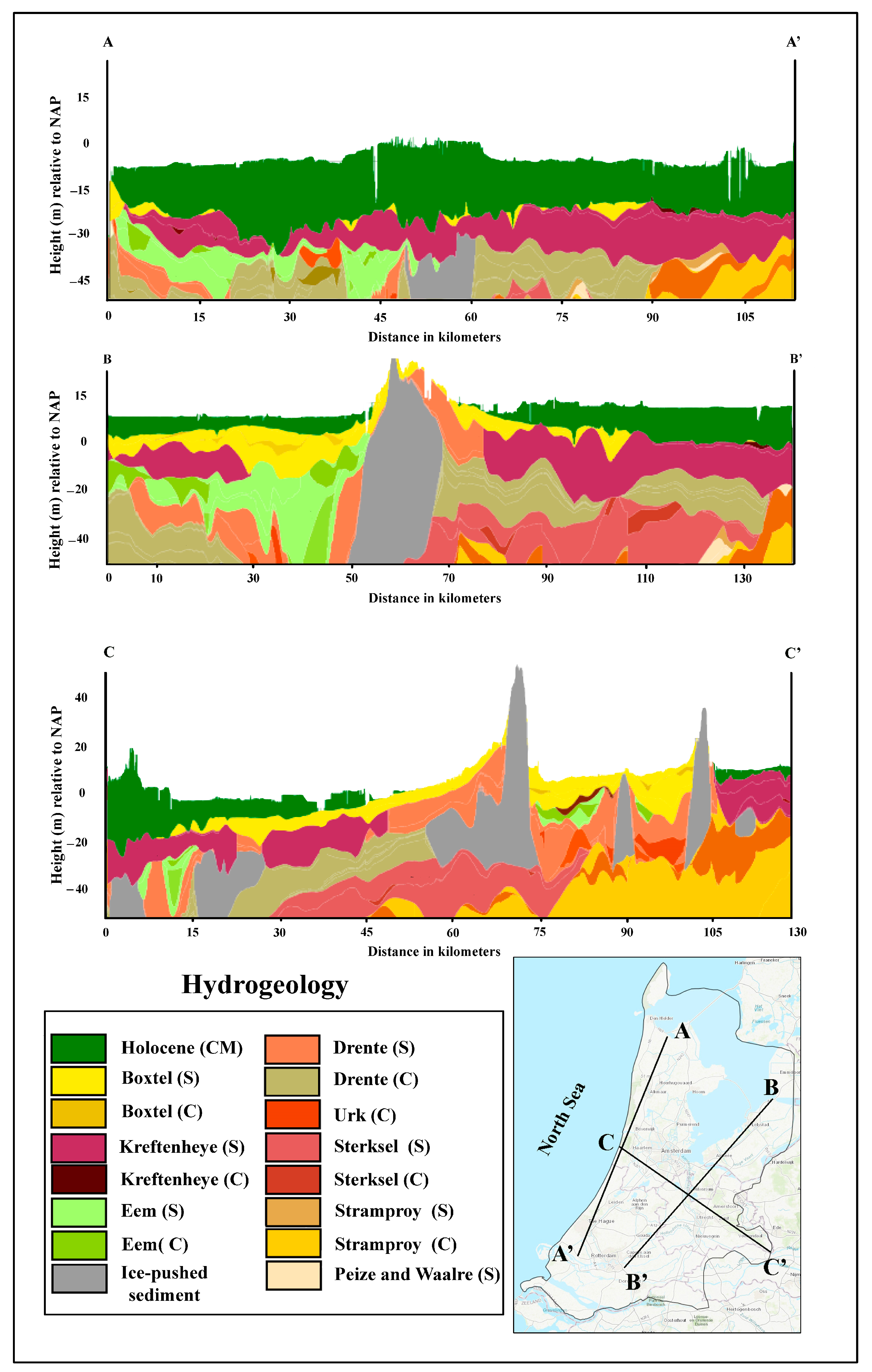
2. Study Area
3. Materials and Methods
3.1. Data Selection
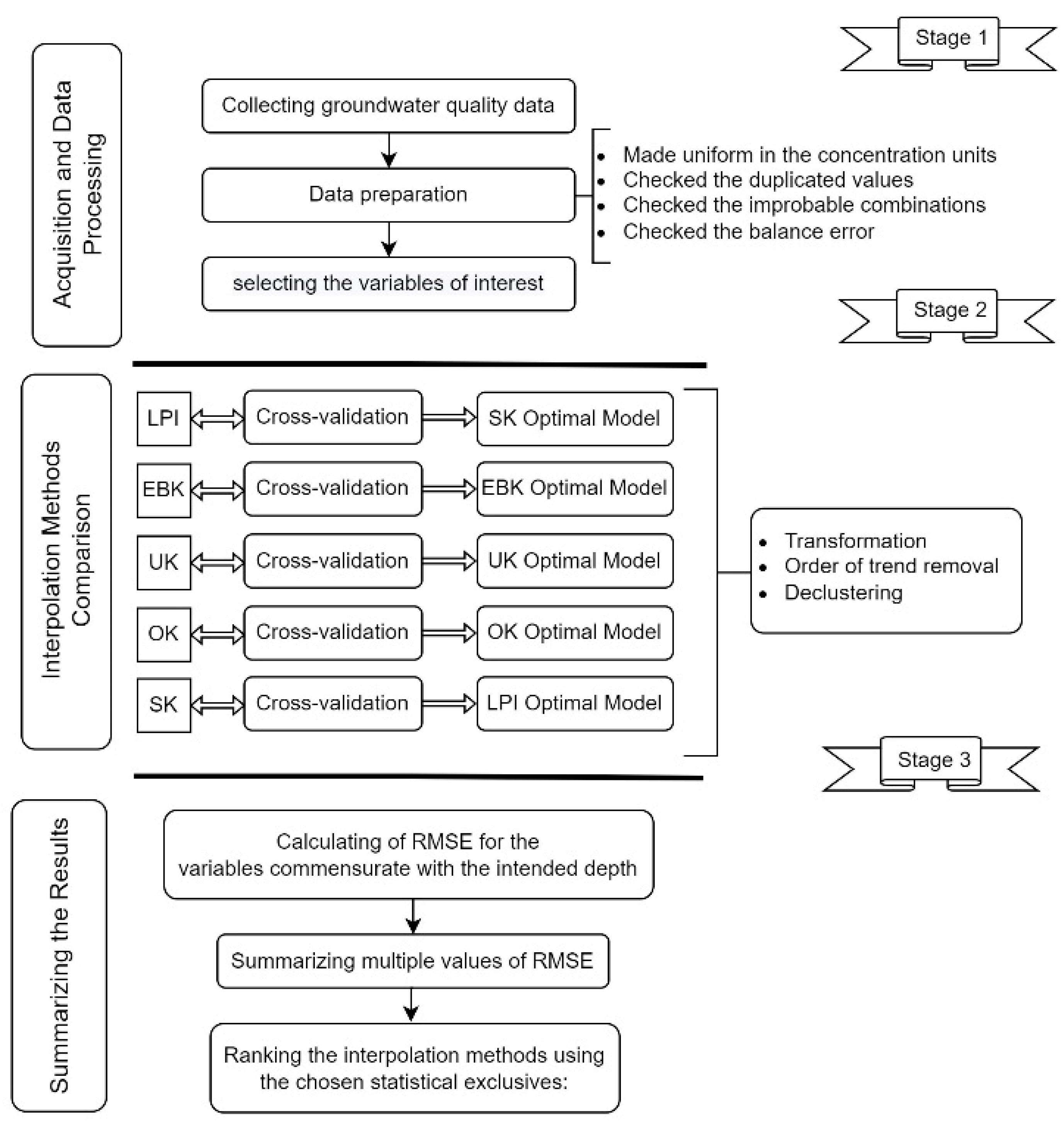
3.2. Methodology
3.3. Interpolation Methods
3.3.1. LPI Method
3.3.2. Classical Kriging Methods
Simple Kriging (SK)
Ordinary Kriging (OK)
Universal Kriging (UK)
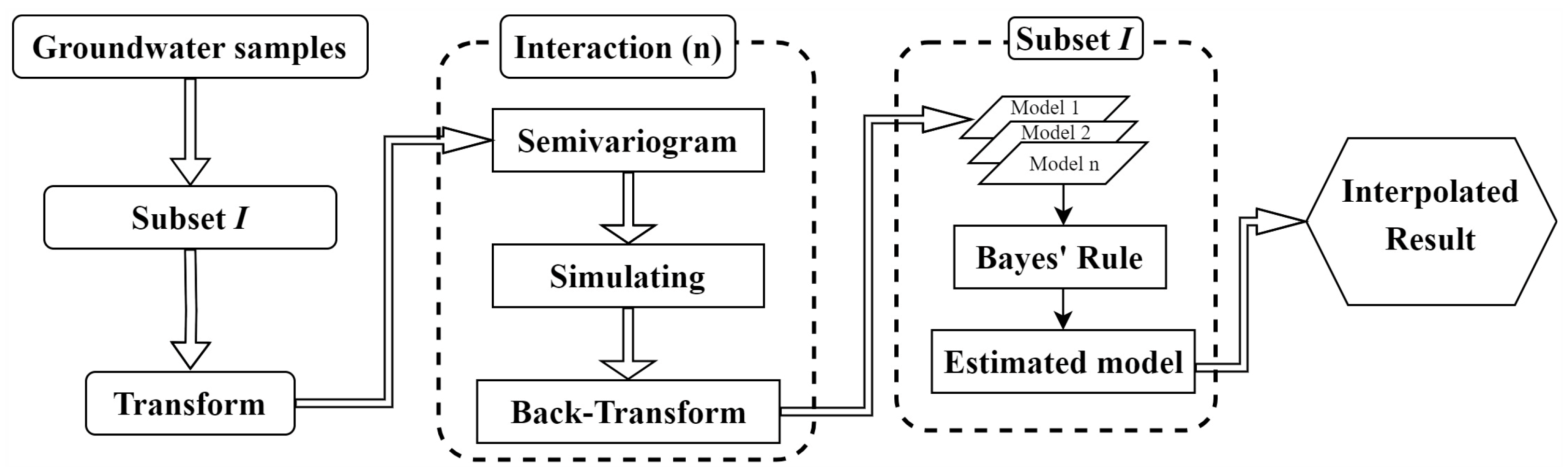
3.3.3. Empirical Bayesian Kriging (EBK)
3.4. Method Strengths and Weaknesses
3.5. Interpolation and Validation
4. Results and Discussion
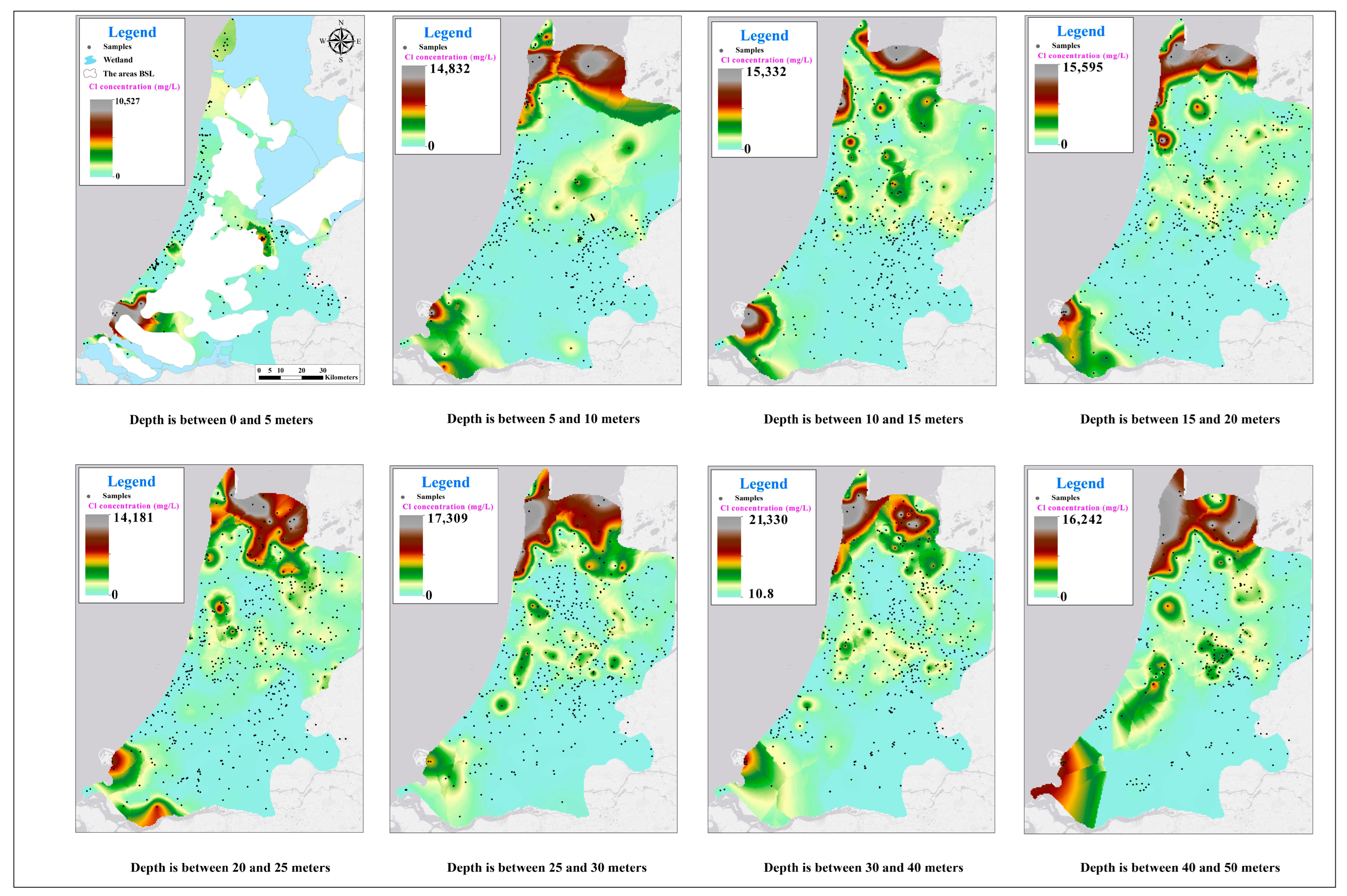
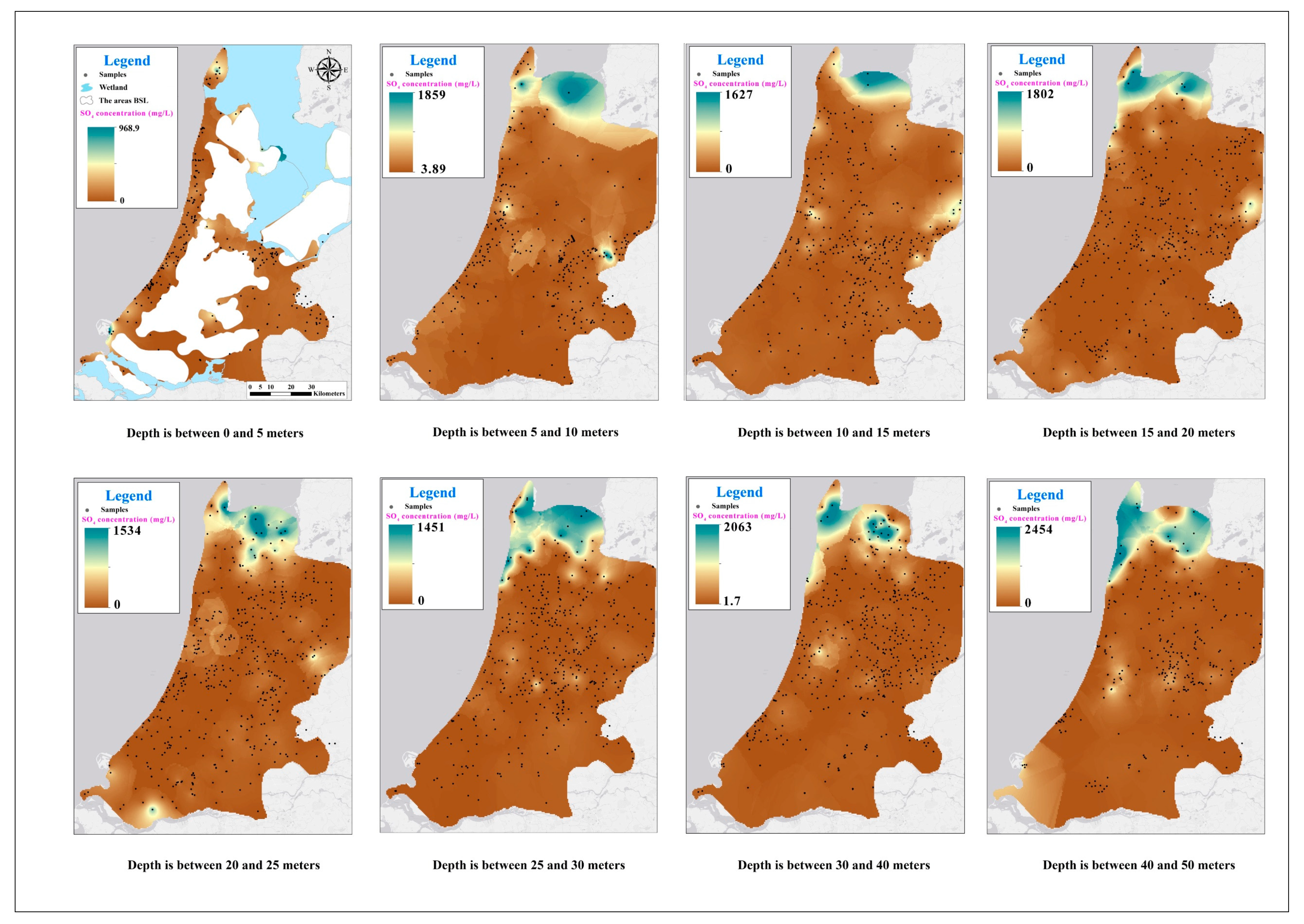
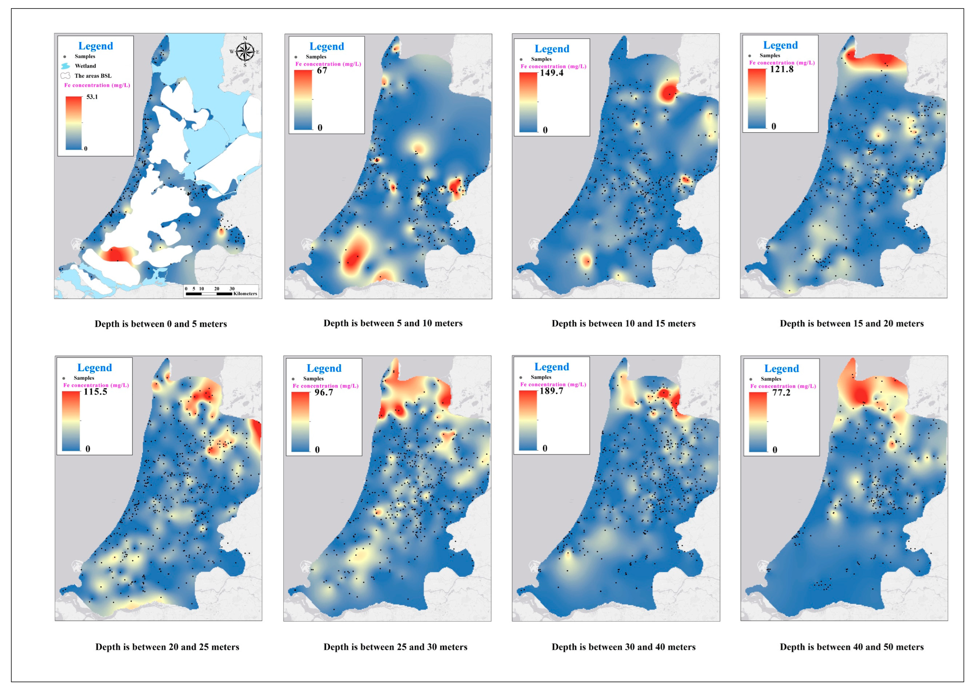
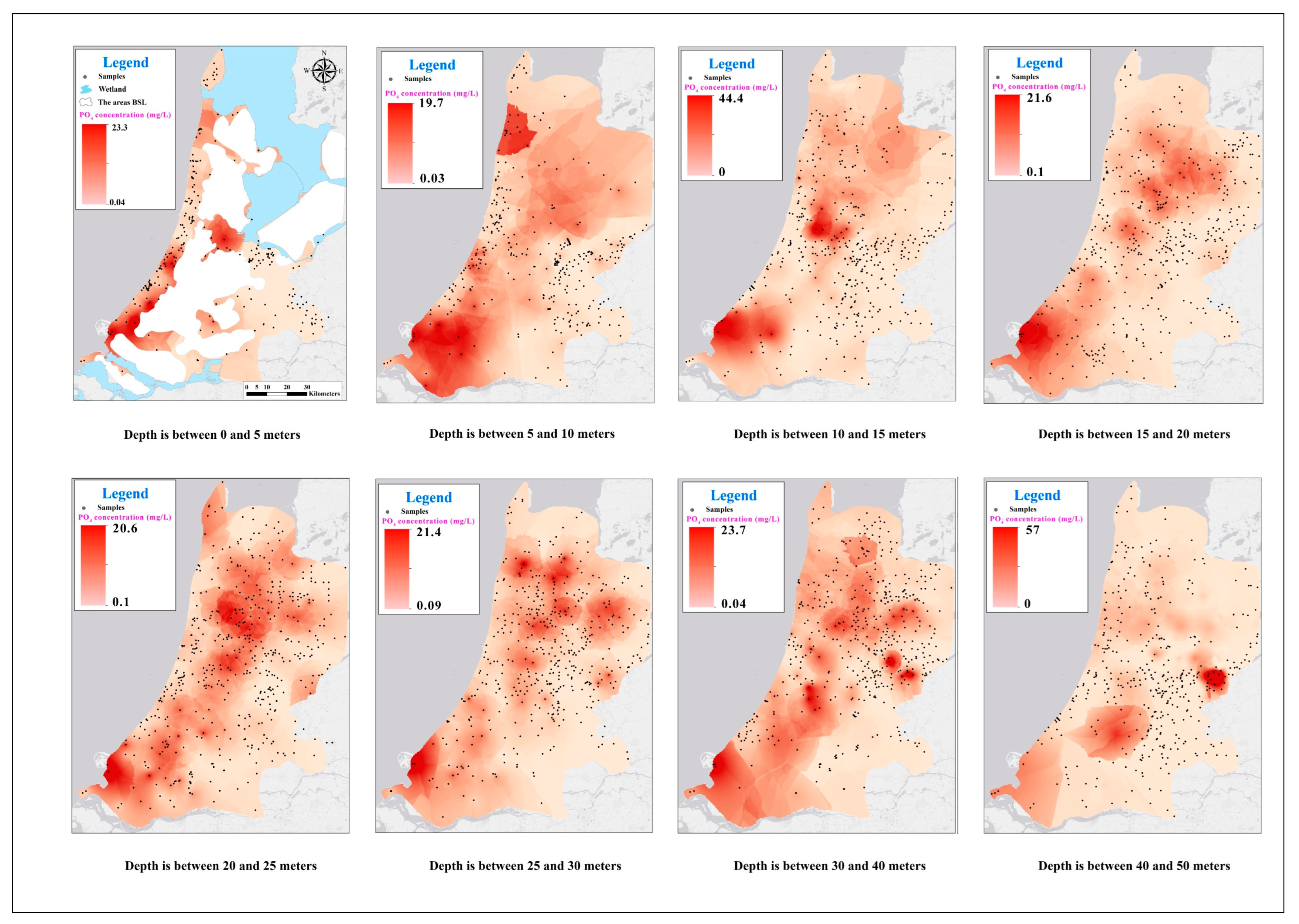
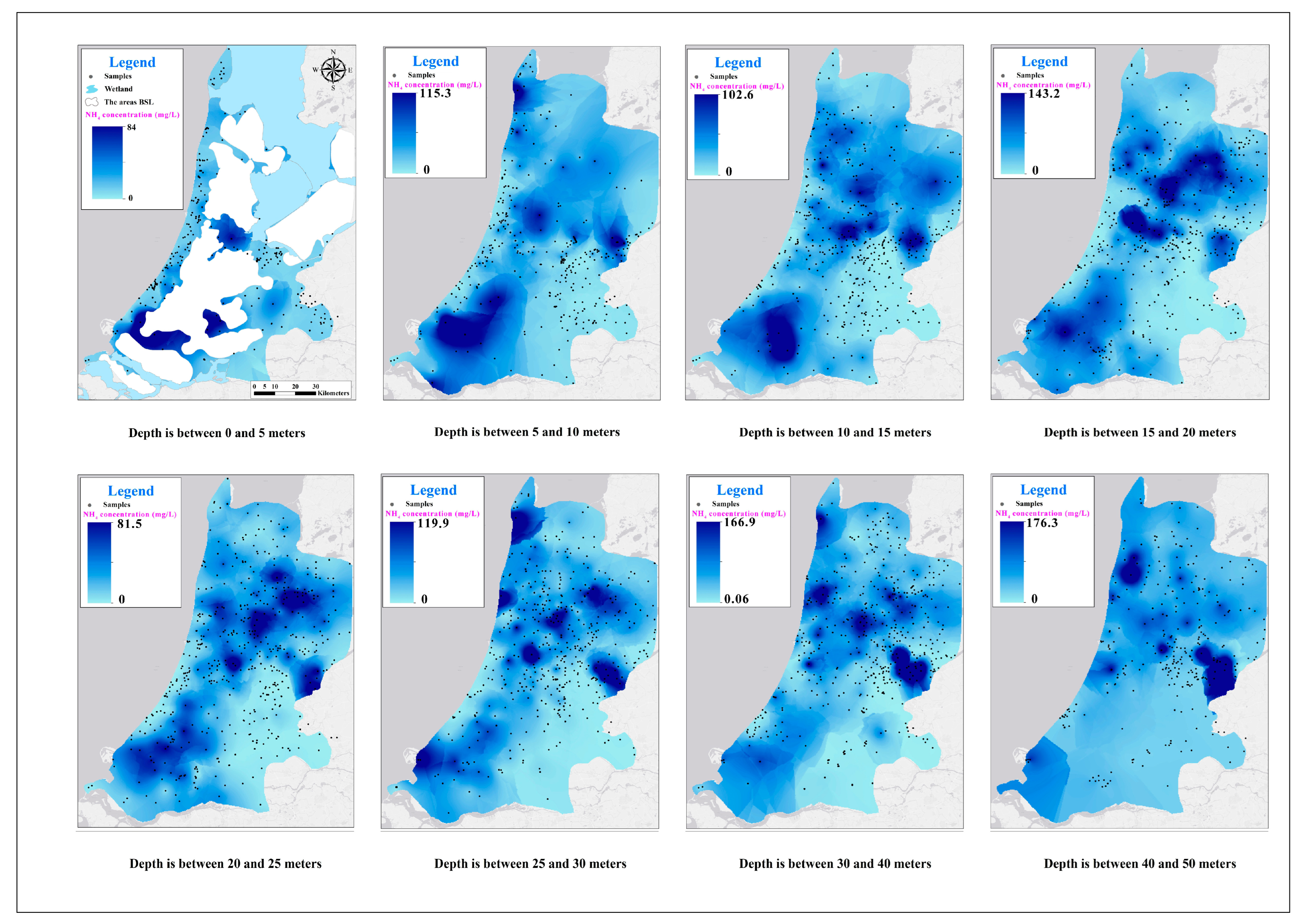
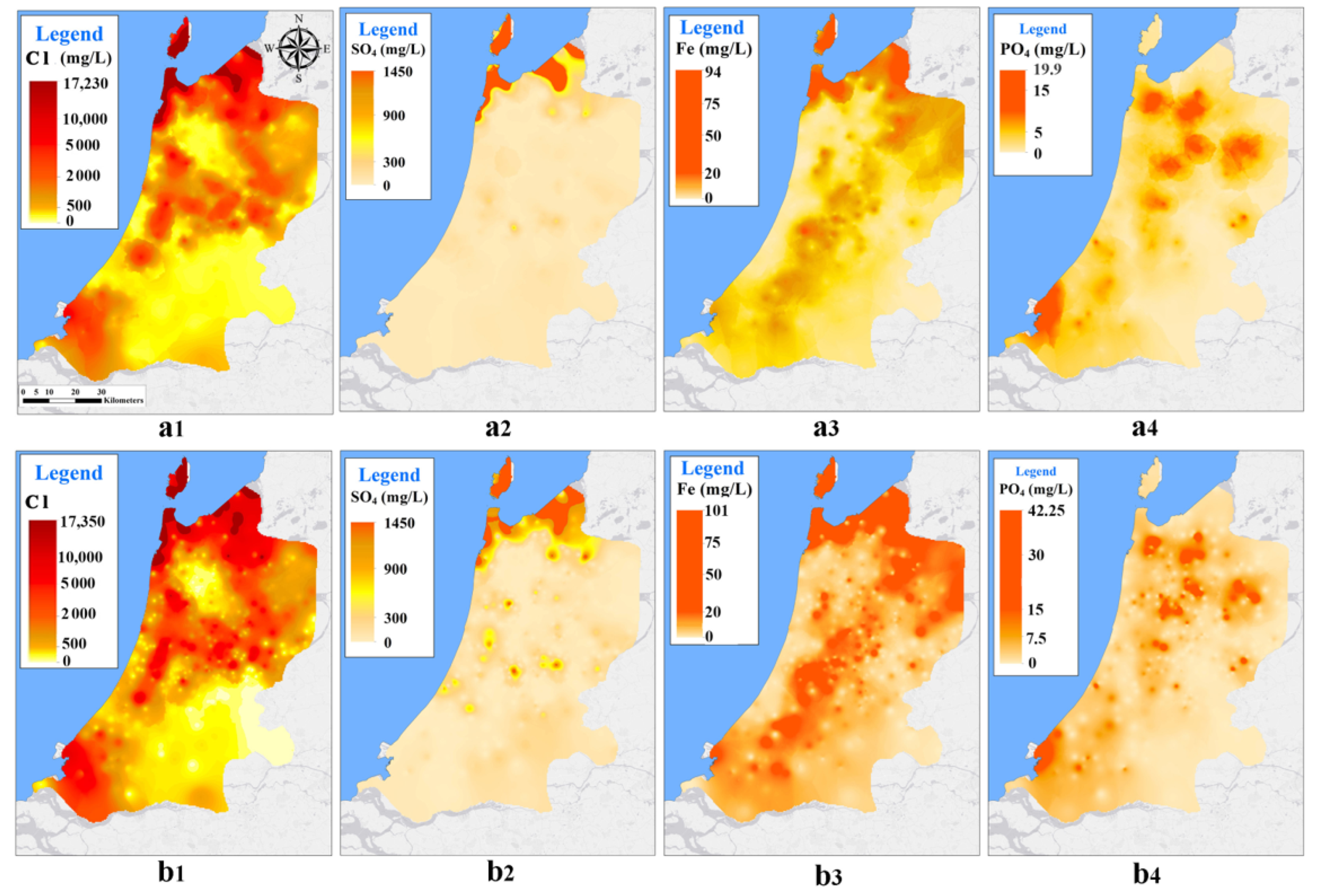
4.1. Maps
4.2. Simulation Accuracy
4.3. Three-Dimensional Aspect
5. Conclusions
Author Contributions
Funding
Data Availability Statement
Acknowledgments
Conflicts of Interest
Appendix A

References
- Zaryab, A.; Nassery, H.R.; Alijani, F. Identifying Sources of Groundwater Salinity and Major Hydrogeochemical Processes in the Lower Kabul Basin Aquifer, Afghanistan. Environ. Sci. Process. Impacts 2021, 23, 1589–1599. [Google Scholar] [CrossRef]
- Gunnink, J.L.; Burrough, P.A. Interactive Spatial Analysis of Soil Attribute Patterns Using Exploratory Data Analysis (EDA) and GIS. In Spatial Analytical Perspectives on GIS; Routledge: Oxford, UK, 2019; pp. 87–100. [Google Scholar]
- De Smith, M.J.; Goodchild, M.F.; Longley, P. Geospatial Analysis: A Comprehensive Guide to Principles, Techniques and Software Tools, 6th ed.; Winchelsea Press: London, UK, 2021; ISBN 9781912556038. [Google Scholar]
- Webster, R.; Oliver, M.A. Geostatistics for Environmental Scientists; John Wiley & Sons: Hoboken, NJ, USA, 2007; ISBN 0470517263. [Google Scholar]
- Smith, J.E.; von Winterfeldt, D. Decision Analysis in Management Science. Manag. Sci. 2004, 50, 561–574. [Google Scholar] [CrossRef]
- Güler, M.; Kara, T. Comparison of Different Interpolation Techniques for Modelling Temperatures in Middle Black Sea Region. Agric. Fac. Gaziosmanpasa Univ. 2014, 31, 61–71. [Google Scholar] [CrossRef]
- Stahl, K.; Moore, R.D.; Floyer, J.A.; Asplin, M.G.; McKendry, I.G. Comparison of Approaches for Spatial Interpolation of Daily Air Temperature in a Large Region with Complex Topography and Highly Variable Station Density. Agric. For. Meteorol. 2006, 139, 224–236. [Google Scholar] [CrossRef]
- Wu, W.; Tang, X.-P.; Ma, X.-Q.; Liu, H.-B. A Comparison of Spatial Interpolation Methods for Soil Temperature over a Complex Topographical Region. Theor. Appl. Clim. 2016, 125, 657–667. [Google Scholar] [CrossRef]
- Hengl, T. A Practical Guide to Geostatistical Mapping, EUR 22904 EN Scientific and Technical Research Series, 2nd ed.; Office for Official Publications of the European Communities: Luxembourg, 2009. [Google Scholar]
- Bhunia, G.S.; Shit, P.K.; Maiti, R. Comparison of GIS-Based Interpolation Methods for Spatial Distribution of Soil Organic Carbon (SOC). J. Saudi Soc. Agric. Sci. 2018, 17, 114–126. [Google Scholar] [CrossRef]
- Murphy, R.R.; Curriero, F.C.; Ball, W.P. Comparison of Spatial Interpolation Methods for Water Quality Evaluation in the Chesapeake Bay. J. Environ. Eng. 2010, 136, 160–171. [Google Scholar] [CrossRef]
- Varouchakis, E.A.; Hristopulos, D.T. Comparison of Stochastic and Deterministic Methods for Mapping Groundwater Level Spatial Variability in Sparsely Monitored Basins. Environ. Monit. Assess. 2013, 185, 1–19. [Google Scholar] [CrossRef]
- Jovein, E.B.; Hosseini, S.M. A Systematic Comparison of Geostatistical Methods for Estimation of Groundwater Salinity in Desert Areas. Iran Water Resour. Res. 2016, 11, 1–15. [Google Scholar]
- Seyedmohammadi, J.; Esmaeelnejad, L.; Shabanpour, M. Spatial Variation Modelling of Groundwater Electrical Conductivity Using Geostatistics and GIS. Model Earth Syst. Environ. 2016, 2, 1–10. [Google Scholar] [CrossRef]
- Xiao, Y.; Gu, X.; Yin, S.; Shao, J.; Cui, Y.; Zhang, Q.; Niu, Y. Geostatistical Interpolation Model Selection Based on ArcGIS and Spatio-Temporal Variability Analysis of Groundwater Level in Piedmont Plains, Northwest China. SpringerPlus 2016, 5, 425. [Google Scholar] [CrossRef]
- Amah, V.E.; Agu, F.A. Geostatistical Modelling of Groundwater Quality at Rumuola Community, Port Harcourt, Nigeria. Asian J. Environ. Ecol. 2020, 12, 37–47. [Google Scholar] [CrossRef]
- Kumari, M.K.N.; Sakai, K.; Kimura, S.; Nakamura, S.; Yuge, K.; Gunarathna, M.H.J.P.; Ranagalage, M.; Duminda, D.M.S. Interpolation Methods for Groundwater Quality Assessment in Tank Cascade Landscape: A Study of Ulagalla Cascade, Sri Lanka. Appl. Ecol. Environ. Res. 2018, 16, 5359–5380. [Google Scholar] [CrossRef]
- Mirzaei, R.; Sakizadeh, M. Comparison of Interpolation Methods for the Estimation of Groundwater Contamination in Andimeshk-Shush Plain, Southwest of Iran. Environ. Sci. Pollut. Res. 2016, 23, 2758–2769. [Google Scholar] [CrossRef]
- Delsman, J.R.; Hu-a-ng, K.R.M.; Vos, P.C.; de Louw, P.G.B.; Oude Essink, G.H.P.; Stuyfzand, P.J.; Bierkens, M.F.P. Paleo-Modeling of Coastal Saltwater Intrusion during the Holocene: An Application to the Netherlands. Hydrol. Earth Syst. Sci. 2014, 18, 3891–3905. [Google Scholar] [CrossRef]
- Griffioen, J.; Vermooten, S.; Janssen, G. Geochemical and Palaeohydrological Controls on the Composition of Shallow Groundwater in the Netherlands. Appl. Geochem. 2013, 39, 129–149. [Google Scholar] [CrossRef]
- Griffioen, J.; Passier, H.F.; Klein, J. Comparison of Selection Methods to Deduce Natural Background Levels for Groundwater Units. Environ. Sci. Technol. 2008, 42, 4863–4869. [Google Scholar] [CrossRef]
- Dufour, F. Groundwater in the Netherlands: Facts and Figures; Netherlands Institute of Applied Geoscience TNO: Delf, The Netherlands, 2000. [Google Scholar]
- Gouw, M.J.P.; Erkens, G. Architecture of the Holocene Rhine-Meuse Delta (The Netherlands)—A Result of Changing External Controls. Neth. J. Geosci. 2007, 86, 23–54. [Google Scholar] [CrossRef]
- De Mulder, E.F.J. Landscapes. In The Netherlands and the Dutch: A Physical and Human Geography; De Mulder, E.F.J., De Pater, B.C., Droogleever Fortuijn, J.C., Eds.; Springer International Publishing: Cham, Switzerland, 2019; pp. 35–58. ISBN 978-3-319-75073-6. [Google Scholar]
- Verschuuren, J. Restoration of Protected Lakes Under Climate Change: What Legal Measures Are Needed to Help Biodiversity Adapt to the Changing Climate? The Case of Lake IJssel, Netherlands. Tilburg Law School Research Paper Forthcoming. Electron. J. 2019. [Google Scholar] [CrossRef]
- Post, V.E.A.; Van der Plicht, H.; Meijer, H.A.J. The Origin of Brackish and Saline Groundwater in the Coastal Area of the Netherlands. Neth. J. Geosci. 2003, 82, 133–147. [Google Scholar] [CrossRef]
- Gribov, A.; Krivoruchko, K. Local Polynomials for Data Detrending and Interpolation in the Presence of Barriers. Stoch. Environ. Res. Risk Assess. 2011, 25, 1057–1063. [Google Scholar] [CrossRef]
- Hani, A.; Abari, S.A.H. Determination of Cd, Zn, K, PH, TNV, Organic Material and Electrical Conductivity (EC) Distribution in Agricultural Soils Using Geostatistics and GIS (Case Study: South-Western of Natanz-Iran). Int. J. Biol. Life Agric. Sci. 2011, 5.0, 264. [Google Scholar] [CrossRef]
- Esri ArcGIS Geostatistical Analyst|Model Spatial Data & Uncertainty. Available online: https://www.esri.com/en-us/arcgis/products/geostatistical-analyst/overview (accessed on 9 November 2021).
- McKillup, S.; Dyar, M.D. Geostatistics Explained: An Introductory Guide for Earth Scientists; Cambridge University Press: Cambridge, UK, 2010. [Google Scholar]
- Abdulmanov, R.; Miftakhov, I.; Ishbulatov, M.; Galeev, E.; Shafeeva, E. Comparison of the Effectiveness of GIS-Based Interpolation Methods for Estimating the Spatial Distribution of Agrochemical Soil Properties. Environ. Technol. Innov. 2021, 24, 101970. [Google Scholar] [CrossRef]
- Krivoruchko, K. Spatial Statistical Data Analysis for GIS Users, 1st ed.; Esri Press: Redlands, CA, USA, 2011; ISBN 978-1-58948-161-9. [Google Scholar]
- Li, J.; Heap, A.D. Spatial Interpolation Methods Applied in the Environmental Sciences: A Review. Environ. Model. Softw. 2014, 53, 173–189. [Google Scholar] [CrossRef]
- ESRI ArcGIS Desktop 10.8 Guide. Available online: https://desktop.arcgis.com/en/arcmap/latest/get-started/setup/arcgis-desktop-quick-start-guide.htm (accessed on 27 November 2021).
- Krivoruchko, K. Empirical Bayesian Kriging. ArcUser Fall 2012, 6, 1145. [Google Scholar]
- Krivoruchko, K.; Fraczek, W. Interpolation of Data Collected along Lines; Esri Press: Redlands, CA, USA, 2015. [Google Scholar]
- Gribov, A.; Krivoruchko, K. Empirical Bayesian Kriging Implementation and Usage. Sci. Total Environ. 2020, 722, 137290. [Google Scholar] [CrossRef]
- Krivoruchko, K.; Gribov, A. Distance Metrics for Data Interpolation over Large Areas on Earth’s Surface. Spat. Stat. 2020, 35, 100396. [Google Scholar] [CrossRef]
- Knotters, M.; Heuvelink, G.B.M. A Disposition of Interpolation Techniques; Wettelijke Onderzoekstaken Natuur & Milieu: Wageningen, Germany, 2010. [Google Scholar]
- Krivoruchko, K.; Butler, K. Unequal Probability-Based Spatial Mapping; Esri Press: Redlands, CA, USA, 2013. [Google Scholar]
- Krivoruchko, K.; Gribov, A. Evaluation of Empirical Bayesian Kriging. Spat. Stat. 2019, 32, 100368. [Google Scholar] [CrossRef]
- Li, Y.; Zhang, M.; Mi, W.; Ji, L.; He, Q.; Xie, S.; Xiao, C.; Bi, Y. Spatial Distribution of Groundwater Fluoride and Arsenic and Its Related Disease in Typical Drinking Endemic Regions. Sci. Total Environ. 2024, 906, 167716. [Google Scholar] [CrossRef]
- Zou, L.; Kent, J.; Lam, N.S.N.; Cai, H.; Qiang, Y.; Li, K. Evaluating Land Subsidence Rates and Their Implications for Land Loss in the Lower Mississippi River Basin. Water 2015, 8, 10. [Google Scholar] [CrossRef]
- Zaresefat, M.; Hosseini, S.; Roudi, M.A. Addressing Nitrate Contamination in Groundwater: The Importance of Spatial and Temporal Understandings and Interpolation Methods. Water 2023, 15, 4220. [Google Scholar] [CrossRef]
- Morris, C.N. Parametric Empirical Bayes Inference: Theory and Applications. J. Am. Stat. Assoc. 1983, 78, 47–55. [Google Scholar] [CrossRef]
- Maritz, J.S.; Lwin, T. Empirical Bayes Methods; CRC Press: Boca Raton, FL, USA, 2018; ISBN 1351071661. [Google Scholar]
- Kumar, N.; Sinha, N.K. Geostatistics: Principles and Applications in Spatial Mapping of Soil Properties. In Geospatial Technologies in Land Resources Mapping, Monitoring and Management; Reddy, G.P.O., Singh, S.K., Eds.; Springer International Publishing: Cham, Switzerland, 2018; pp. 143–159. ISBN 978-3-319-78711-4. [Google Scholar]
- Sahu, S.K. Bayesian Modeling of Spatio-Temporal Data with R; CRC: New York, NY, USA, 2022. [Google Scholar]
- van Lieshout, M.N.M. Theory of Spatial Statistics: A Concise Introduction; CRC: New York, NY, USA, 2019. [Google Scholar]
- Li, J.; Heap, A.D. A Review of Spatial Interpolation Methods for Environmental Scientists. Geosci. Aust. 2008, 23, 137. [Google Scholar]
- Boumpoulis, V.; Michalopoulou, M.; Depountis, N. Comparison between Different Spatial Interpolation Methods for the Development of Sediment Distribution Maps in Coastal Areas. Earth Sci. Inform. 2023, 16, 2069–2087. [Google Scholar] [CrossRef]
- Tomlinson, K.M. A Spatial Evaluation of Groundwater Quality Salinity and Underground Injection Controlled Well Activity in Texas. Ph.D. Thesis, The University of Texas, Dallas, TX, USA, 2019. [Google Scholar]
- Ahmad, A.Y.; Saleh, I.A.; Balakrishnan, P.; Al-Ghouti, M.A. Comparison GIS-Based Interpolation Methods for Mapping Groundwater Quality in the State of Qatar. Groundw. Sustain. Dev. 2021, 13, 100573. [Google Scholar] [CrossRef]
- Xie, Y.; Chen, T.; Lei, M.; Yang, J.; Guo, Q.; Song, B.; Zhou, X. Spatial Distribution of Soil Heavy Metal Pollution Estimated by Different Interpolation Methods: Accuracy and Uncertainty Analysis. Chemosphere 2011, 82, 468–476. [Google Scholar] [CrossRef] [PubMed]
- van den Brink, C.; Frapporti, G.; Griffioen, J.; Zaadnoordijk, W.J. Statistical Analysis of Anthropogenic versus Geochemical-Controlled Differences in Groundwater Composition in The Netherlands. J. Hydrol. 2007, 336, 470–480. [Google Scholar] [CrossRef]
- Van Dam, H. Evaluatie Basismeetnet Waterkwaliteit Hollands Noorderkwartier: Trendanalyse Hydrobiologie, Temperatuur En Waterchemie 1982–2007; Water en Natuur: Amsterdam, The Netherlands, 2009. [Google Scholar]
- Buijsman, E.; Aben, J.M.M.; Hetteling, J.P.; Van Hinsberg, A.; Koelemeijer, R.B.A.; Maas, R.J.M. Zure Regen, Een Analyse van Dertig Jaar Verzuringsproblematiek in Nederland; Planbureau voor de Leefomgeving (PBL): The Hague, The Netherlands, 2010. [Google Scholar]
- Liu, R.; Chen, Y.; Sun, C.; Zhang, P.; Wang, J.; Yu, W.; Shen, Z. Uncertainty Analysis of Total Phosphorus Spatial–Temporal Variations in the Yangtze River Estuary Using Different Interpolation Methods. Mar. Pollut. Bull. 2014, 86, 68–75. [Google Scholar] [CrossRef]
- Falivene, O.; Cabrera, L.; Tolosana-Delgado, R.; Sáez, A. Interpolation Algorithm Ranking Using Cross-Validation and the Role of Smoothing Effect. A Coal Zone Example. Comput. Geosci. 2010, 36, 512–519. [Google Scholar] [CrossRef]
- REGIS model Subsurface Models|DINO Counter. Available online: https://www.dinoloket.nl/ondergrondmodellen (accessed on 28 November 2022).
- Jirner, E.; Johansson, P.-O.; McConnachie, D.; Burt, A.; Peter, P.M.; Tomlinson, J.; Lawson, A.K.; Vernes, R.W.; Dabekaussen, W.; Gunnink, J.L.; et al. Application Theme 2—Groundwater Evaluations. In Applied Multidimensional Geological Modeling: Informing Sustainable Human Interactions with the Shallow Subsurface; John, Wiley & Sons: Hoboken, NJ, USA, 2021; pp. 457–477. [Google Scholar] [CrossRef]
- Arora, B.; Mohanty, B.P.; McGuire, J.T. An Integrated Markov Chain Monte Carlo Algorithm for Upscaling Hydrological and Geochemical Parameters from Column to Field Scale. Sci. Total Environ. 2015, 512–513, 428–443. [Google Scholar] [CrossRef]
- Appelo, C.A.J.; Willemsen, A. Geochemical Calculations and Observations on Salt Water Intrusions, I. A Combined Geochemical/Minxing Cell Model. J. Hydrol. 1987, 94, 313–330. [Google Scholar] [CrossRef]
- Post, V.E.A.; Kooi, H. Rates of Salinization by Free Convection in High-Permeability Sediments: Insights from Numerical Modeling and Application to the Dutch Coastal Area. Hydrogeol. J. 2003, 11, 549–559. [Google Scholar] [CrossRef]
- Yu, X.; Michael, H.A. Impacts of the Scale of Representation of Heterogeneity on Simulated Salinity and Saltwater Circulation in Coastal Aquifers. Water Resour. Res. 2022, 58, e2020WR029523. [Google Scholar] [CrossRef]
- Rata, M.; Douaoui, A.; Larid, M.; Douaik, A. Comparison of Geostatistical Interpolation Methods to Map Annual Rainfall in the Chéliff Watershed, Algeria. Theor. Appl. Clim. 2020, 141, 1009–1024. [Google Scholar] [CrossRef]
- Allen, D.M.; Schuurman, N.; Zhang, Q. Using Fuzzy Logic for Modeling Aquifer Architecture. J. Geogr. Syst. 2007, 9, 289–310. [Google Scholar] [CrossRef]
- Burke, H.F.; Ford, J.R.; Hughes, L.; Thorpe, S.; Lee, J.R. A 3D Geological Model of the Superficial Deposits in the Selby Area; CR/17/112N; British Geological Survey: Nottingham, UK, 2017.
- Turner, A.K.; Kessler, H.; van der Meulen, M.J. Applied Multidimensional Geological Modeling: Informing Sustainable Human Interactions with the Shallow Subsurface; John Wiley & Sons: Hoboken, NJ, USA, 2021; ISBN 1119163102. [Google Scholar]


| Method | Advantages | Disadvantages | Influencing Parameters | Differences in Estimated Results |
|---|---|---|---|---|
| LPI | Adapts to local patterns, no stationarity assumptions, efficient | No uncertainty quantification, overfitting risk | Polynomial degree, smoothing, neighbourhood | Lower error in areas with local variations, higher in smoother regions |
| SK | Simple, unbiased predictions | Assumes constant mean, no uncertainty | Semivariogram, data quality | Higher RMSE when constant mean assumption fails |
| OK | Spatial dependence, minimises error, predicts uncertainty | Requires stationarity, complex semivariogram model | Nugget 1 effect, Sill 2, Range 3 Data quality | Lower error with local mean adaptation, affected by semivariogram choice. |
| UK | Handles trends, improves non-stationary data, predicts uncertainty | Complex, trend requirements, overfitting risk | Semivariogram, trend model, data quality | Lower error with trends, higher if trends are misidentified |
| EBK | Automates parameter estimation, handles non-stationarity | Potential bias, limited control, intensive | Simulations, data quality, distribution | Lower error with variability, higher with lower data density |
| Depth Interval (m-NAP) | Count | Median, Mean and Interquartile Range (mg/L) | ||||||||||||||
|---|---|---|---|---|---|---|---|---|---|---|---|---|---|---|---|---|
| Cl | SO4 | Fe | PO4 | NH4 | ||||||||||||
| 0 to 5 | 249 | 78 | 355 | 113 | 35 | 64 | 57 | 1.9 | 4.4 | 5.6 | 0.5 | 2.6 | 2.0 | 1.0 | 4.0 | 3.1 |
| 5 to 10 | 360 | 121 | 844 | 286 | 37 | 104 | 85 | 3.4 | 6.8 | 8.1 | 0.9 | 3.1 | 3.0 | 3.1 | 10.0 | 12.2 |
| 10 to 15 | 455 | 147 | 919 | 667 | 17 | 81 | 68 | 4.6 | 9.2 | 10.0 | 1.2 | 3.7 | 3.2 | 5.0 | 13.0 | 15.9 |
| 15 to 20 | 462 | 191 | 1000 | 1002 | 11 | 67 | 40 | 5.6 | 10.9 | 14.1 | 1.5 | 3.8 | 4.2 | 8.3 | 15.4 | 18.9 |
| 20 to 25 | 519 | 175 | 1159 | 1170 | 11 | 82 | 43 | 6.1 | 11.5 | 13.1 | 1.3 | 3.5 | 4.2 | 8.8 | 15.0 | 21.3 |
| 25 to 30 | 485 | 257 | 1224 | 1330 | 8 | 73 | 41 | 6.9 | 11.2 | 12.5 | 1.2 | 3.2 | 3.7 | 8.8 | 14.0 | 17.0 |
| 30 to 40 | 503 | 544 | 1617 | 1926 | 16 | 108 | 55 | 6.9 | 11.9 | 12.6 | 0.9 | 2.4 | 2.4 | 6.7 | 12.9 | 14.1 |
| 40 to 50 | 317 | 623 | 2180 | 2863 | 17 | 137 | 69 | 5.4 | 9.6 | 11.3 | 0.6 | 2.0 | 1.5 | 5.5 | 11.4 | 10.2 |
| Method | 0 to 5 | 5 to 10 | 10 to 15 | 15 to 20 | 20 to 25 | 25 to 30 | 30 to 40 | 40 to 50 | |
|---|---|---|---|---|---|---|---|---|---|
| Depth | |||||||||
| Chloride | |||||||||
| SK | 899 | 1698 | 1659 | 1610 | 1963 | 1367 | 1810 | 1684 | |
| OK | 1067 | 1816 | 1506 | 1511 | 1477 | 1207 | 1767 | 1367 | |
| UK | 1116 | 1816 | 1690 | 1473 | 1477 | 1250 | 1846 | 1464 | |
| EBK | 986 | 1537 | 1427 | 1470 | 1430 | 1169 | 1487 | 1351 | |
| IDW | 1063 | 1596 | 1420 | 1481 | 1504 | 1224 | 1778 | 1427 | |
| Sulphate | |||||||||
| SK | 119 | 216 | 165 | 184 | 169 | 180 | 206 | 165 | |
| OK | 115 | 225 | 150 | 167 | 173 | 133 | 212 | 215 | |
| UK | 122 | 218 | 162 | 173 | 180 | 135 | 203 | 217 | |
| EBK | 128 | 210 | 129 | 167 | 171 | 142 | 209 | 163 | |
| IDW | 124 | 216 | 130 | 163 | 172 | 141 | 206 | 172 | |
| Ammonium | |||||||||
| SK | 8.1 | 15.6 | 13.2 | 13.1 | 10.5 | 13.5 | 14.9 | 25 | |
| OK | 7.07 | 12.3 | 13.57 | 13.1 | 10.1 | 14.4 | 15.4 | 21.7 | |
| UK | 7.19 | 12.4 | 13.6 | 13.1 | 10.8 | 13.7 | 15.7 | 21.8 | |
| EBK | 7.1 | 12.2 | 13.1 | 12.9 | 9.1 | 13.4 | 14.8 | 21 | |
| IDW | 7.5 | 12.5 | 13.4 | 13.1 | 9.4 | 13.5 | 15.4 | 22 | |
| Iron | |||||||||
| SK | 6.71 | 9.1 | 12.2 | 12.5 | 10.4 | 11.2 | 14.5 | 7.2 | |
| OK | 7.1 | 9.5 | 12.4 | 12.4 | 10.58 | 10.1 | 15.1 | 7.8 | |
| UK | 7.1 | 9.3 | 11.5 | 12.4 | 10.5 | 9.49 | 14.6 | 7.88 | |
| EBK | 6.3 | 9.1 | 11.1 | 12.3 | 10.2 | 9.1 | 14.4 | 7 | |
| IDW | 6.8 | 9.7 | 11.6 | 12.2 | 9.9 | 9.5 | 14.9 | 7 | |
| Phosphate | |||||||||
| SK | 4.3 | 6 | 5.16 | 5.95 | 3.9 | 4.3 | 3.61 | 4.3 | |
| OK | 4.4 | 6.2 | 5.45 | 4.7 | 3.9 | 4.3 | 3.7 | 5 | |
| UK | 4.5 | 6.2 | 5.45 | 4.8 | 3.8 | 4.38 | 3.7 | 4.3 | |
| EBK | 4 | 6.05 | 4.9 | 4.6 | 3.8 | 4.2 | 3.5 | 4.3 | |
| IDW | 4.43 | 6.16 | 5.44 | 4.9 | 4.08 | 4.49 | 3.8 | 4.78 | |
Disclaimer/Publisher’s Note: The statements, opinions and data contained in all publications are solely those of the individual author(s) and contributor(s) and not of MDPI and/or the editor(s). MDPI and/or the editor(s) disclaim responsibility for any injury to people or property resulting from any ideas, methods, instructions or products referred to in the content. |
© 2024 by the authors. Licensee MDPI, Basel, Switzerland. This article is an open access article distributed under the terms and conditions of the Creative Commons Attribution (CC BY) license (https://creativecommons.org/licenses/by/4.0/).
Share and Cite
Zaresefat, M.; Derakhshani, R.; Griffioen, J. Empirical Bayesian Kriging, a Robust Method for Spatial Data Interpolation of a Large Groundwater Quality Dataset from the Western Netherlands. Water 2024, 16, 2581. https://doi.org/10.3390/w16182581
Zaresefat M, Derakhshani R, Griffioen J. Empirical Bayesian Kriging, a Robust Method for Spatial Data Interpolation of a Large Groundwater Quality Dataset from the Western Netherlands. Water. 2024; 16(18):2581. https://doi.org/10.3390/w16182581
Chicago/Turabian StyleZaresefat, Mojtaba, Reza Derakhshani, and Jasper Griffioen. 2024. "Empirical Bayesian Kriging, a Robust Method for Spatial Data Interpolation of a Large Groundwater Quality Dataset from the Western Netherlands" Water 16, no. 18: 2581. https://doi.org/10.3390/w16182581