
Flood Susceptibility Assessment for Improving the Resilience Capacity of Railway Infrastructure Networks

 , , , ,
  , ,
, ,  and
and
Abstract
:1. Introduction
Background
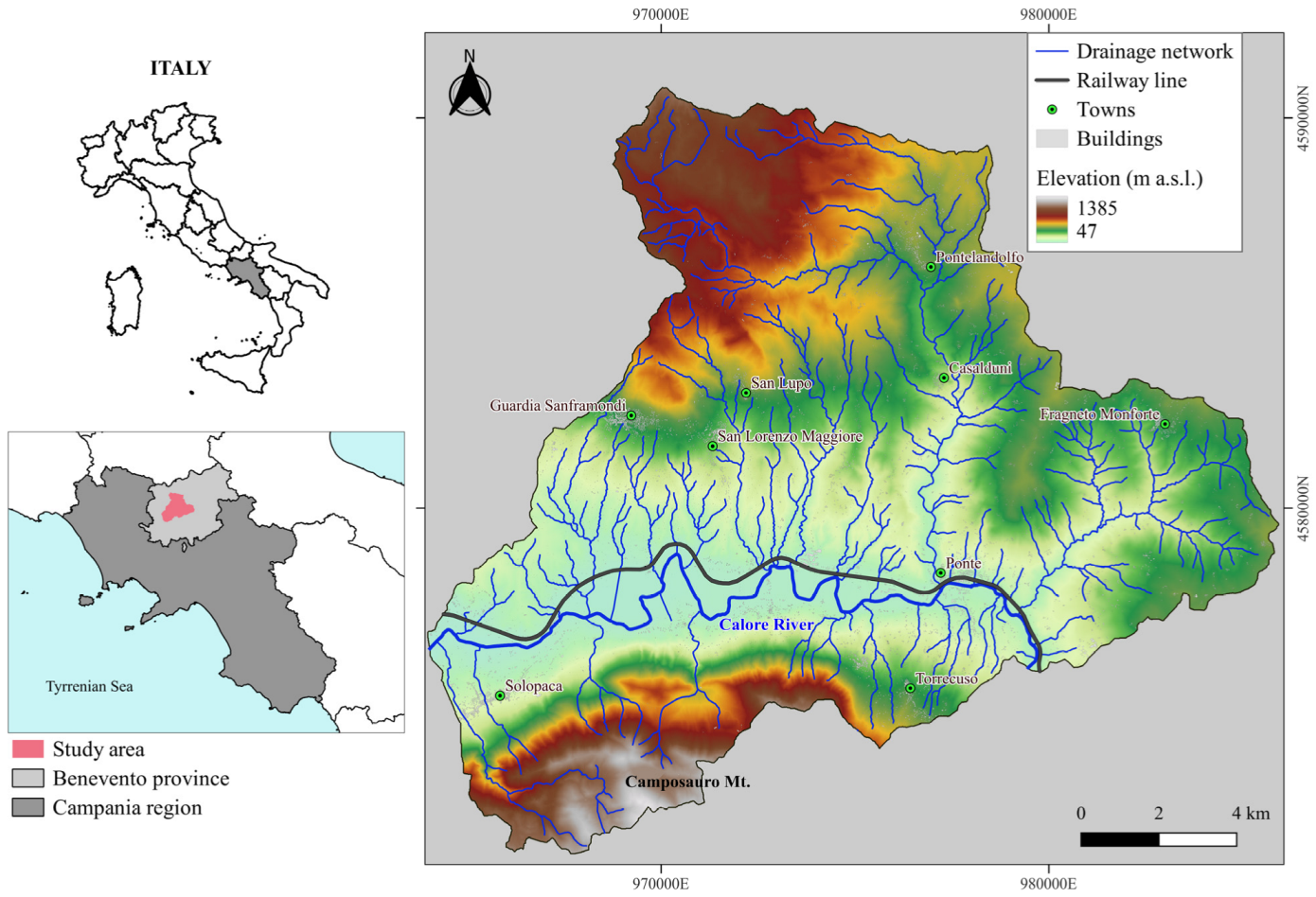
2. Case Study
3. Methodology
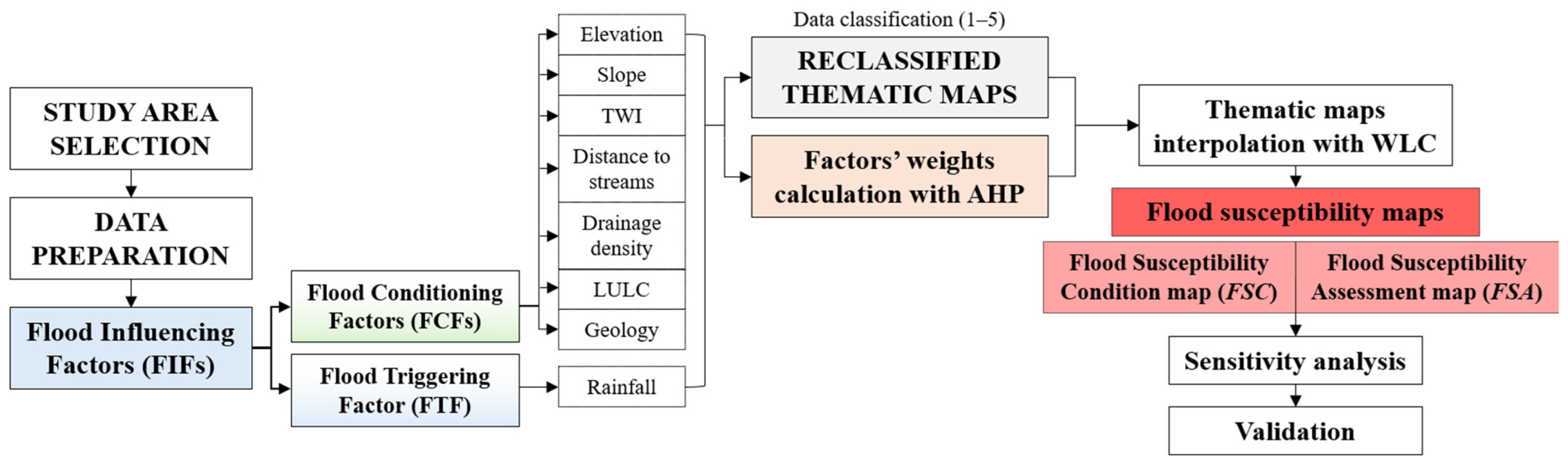
3.1. Methodology Flowchart
- -
- The data required for the analysis were collected from various sources and pre-processed in GIS.
- -
- Several flood-influencing factors (FIFs) covering hydrological, geomorphological, environmental, topographical, and meteorological conditions, based on the actual characteristics of the study area, were selected. Input data for each factor were resampled in the GIS environment as raster data with 10 m spatial resolution, resulting in 4,306,822 cells (2194 columns, 1963 rows), and reprojected in the reference system WGS 84/UTM zone 32 N. We classify the FIFs into seven static flood-conditioning factors (FCFs: elevation, slope, topographic wetness index, distance to streams, drainage density, land use/land cover and geology) and one dynamic flood-triggering factor (FTF, October 2015 rainfall). Due to the diverse nature of each factor, all the thematic maps were reclassified on a scale from 1 to 5 (rating score), where 1 refers to a very low (or negligible) level of influence/susceptibility to flooding and 5 to a very high level. The approach of setting a priori the number of susceptibility classes is also employed in similar studies for identifying flood-prone areas [38,42,56,60,70,71,72,73].
- -
- The AHP technique was employed to determine the relative weights of the flood-influencing factors.
- -
- The thematic map layers were superposed in GIS using the weights calculated with the AHP technique. A flood susceptibility condition map (FSC) was created by combining the seven FCFs with their weights, and a flood susceptibility assessment map (FSA) was obtained by combining the seven FCFs and the one FTF (rainfall) with their weights. The pixel value of each output map (FSi) was obtained using the following equation (weighted linear combination, WLC, [74]):
- -
- A sensitivity analysis was applied to both the FSC and FSA maps to evaluate the influence of uncertainties of the input factors’ weights on the derived flood susceptibility maps.
- -
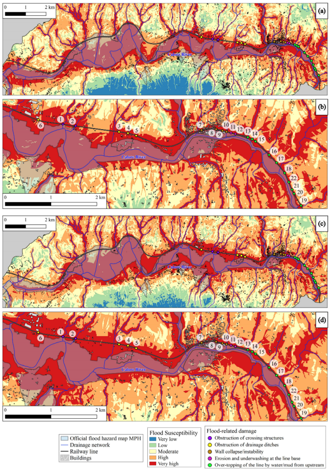
- To validate the flood susceptibility zonation method, historical flood-related damage sites on the railway infrastructure from the railway company and official flood inundation maps from the competent authorities were used.
3.2. Flood-Influencing Factors (FIFs)
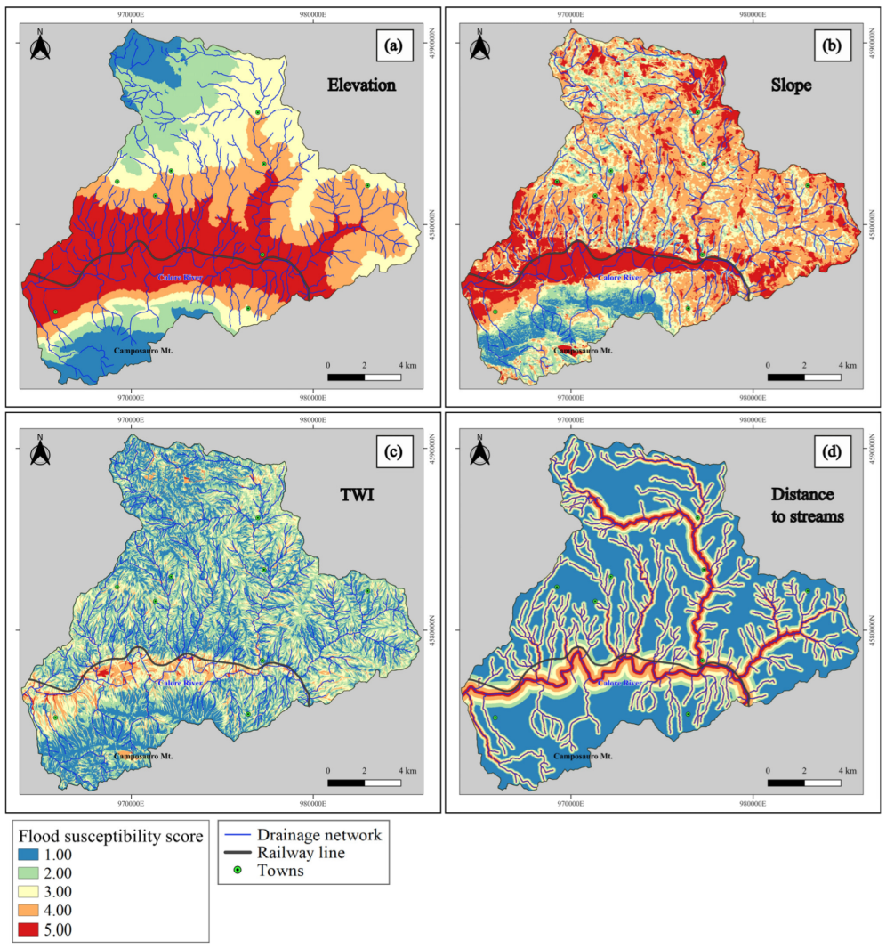
3.2.1. Elevation (E)
3.2.2. Slope Angle (S)
3.2.3. Topographic Wetness Index (TWI)
3.2.4. Distance to Streams (DS)
3.2.5. Drainage Density (DD)
3.2.6. Geology (G)
3.2.7. Land Use Land Cover (LULC)
3.2.8. Cumulative Two-Day Rainfall (C2DR)
3.3. Calculation of Weights
4. Map Interpolation and Sensitivity Analysis
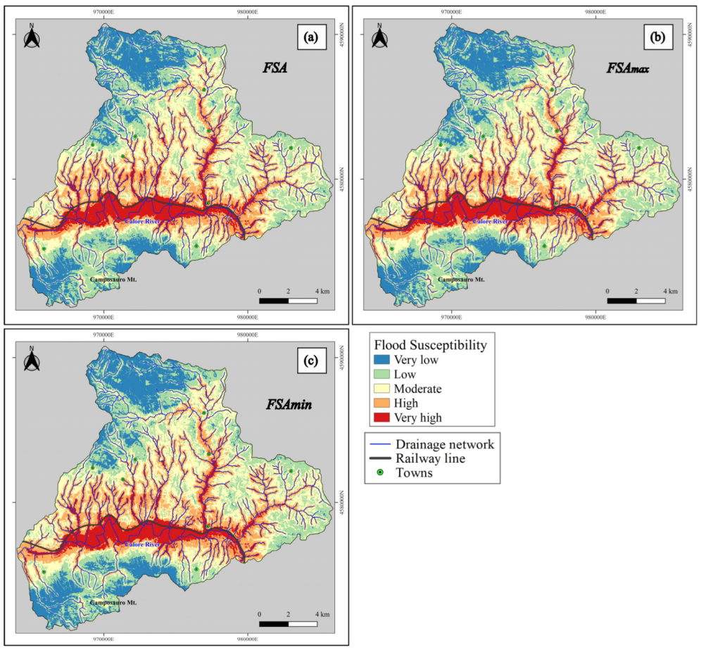
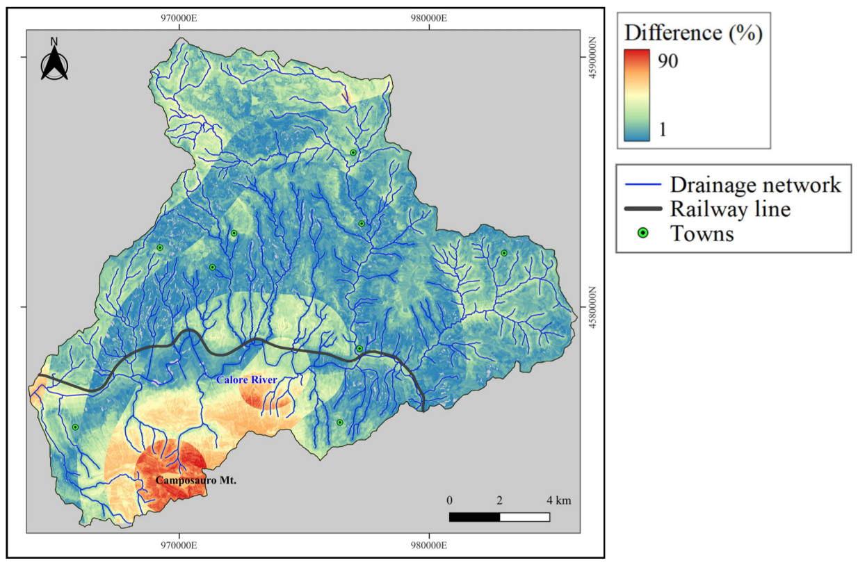
Sensitivity Analysis
5. Results and Discussion
5.1. Spatial Variation of Flood Susceptibility at Basin Level
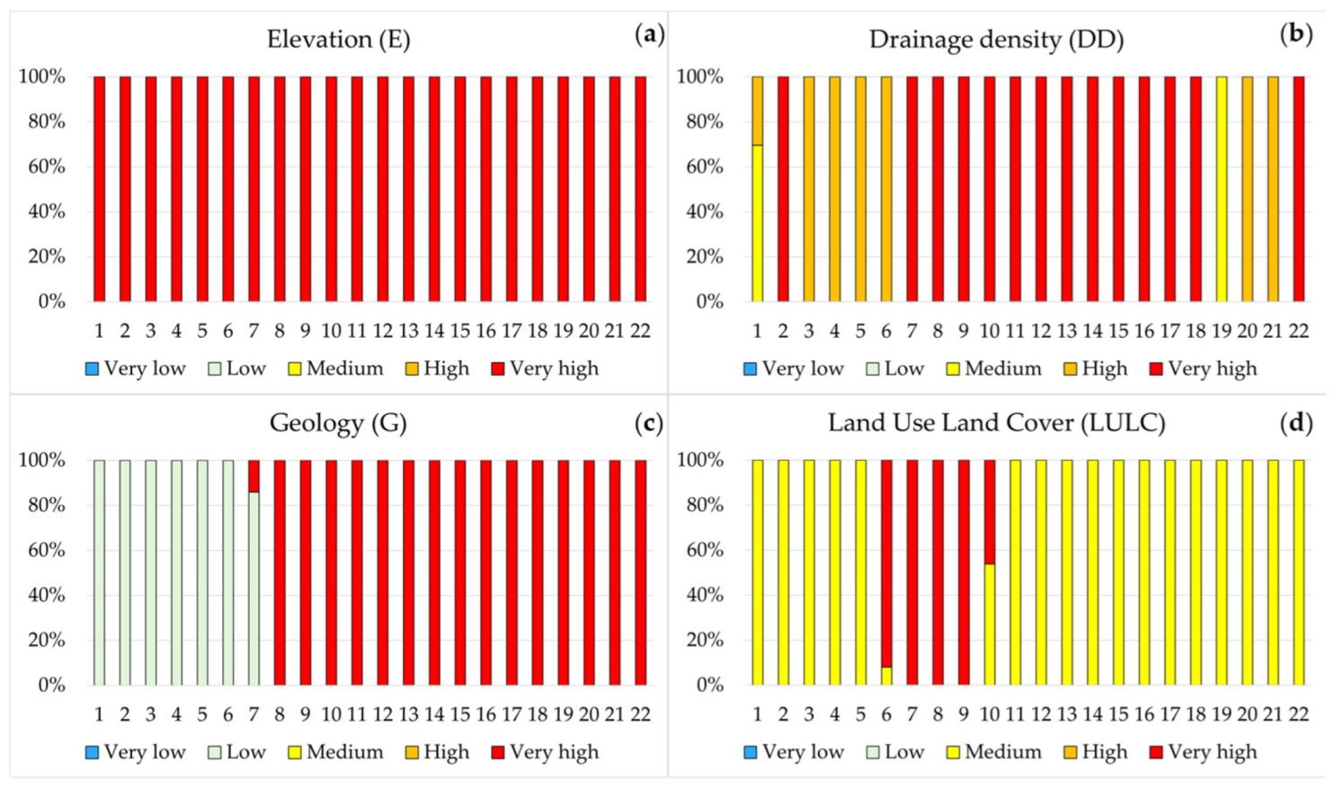
5.2. Impact of Factors on the Flood Susceptibility Distribution
5.3. Validation of the Methodology
5.4. Limitations and Future Research Directions
- -
- The inherent subjectivity in expert assessments within the analytic hierarchy process (AHP) can lead to biases in the weighting of criteria, even though pairwise comparisons are used to promote consistency. The influence of this bias can be assessed with sensitivity analysis conducted on weights.
- -
- The accuracy and resolution of the input data could introduce uncertainties, particularly in regions with complex topography or diverse land cover. Depending on the scope of the susceptibility map, different scales could be required for different applications.
- -
- The present application considers the rainfall forcing from the 2015 autumn event only. There is the potential to include present climate (rainfalls with different durations and intensity) and future projections where available.
- -
- The extent and nature of present land use and land cover (LULC) do not account for historical modifications or predict future changes. Future developments of the territory should be included if the corresponding information is available.
6. Conclusions
Author Contributions
Funding
Data Availability Statement
Acknowledgments
Conflicts of Interest
Appendix A. Analytical Hierarchy Process (AHP)
Appendix A.1. Development of the Pairwise Comparison Matrix

| Intensity of Importance | Values for Reciprocal Scale | Definition |
|---|---|---|
| 1 | 1 | Equal importance |
| 2 | 1/2 | Equal to moderate importance |
| 3 | 1/3 | Moderate importance |
| 4 | 1/4 | Moderate to strong importance |
| 5 | 1/5 | Strong importance |
| 6 | 1/6 | Strong to very strong importance |
| 7 | 1/7 | Very strong importance |
| 8 | 1/8 | Very to extremely strong importance |
| 9 | 1/9 | Extreme importance |
| Pairwise Comparison Matrix | |||||||
|---|---|---|---|---|---|---|---|
| Factor | S | DS | TWI | E | DD | G | LULC |
| Slope (S) | 1 | 1 | 2 | 2 | 3 | 4 | 5 |
| Distance from streams (DS) | 1 | 1 | 2 | 2 | 3 | 4 | 5 |
| Topographic wetness index (TWI) | 1/2 | 1/2 | 1 | 1 | 2 | 3 | 4 |
| Elevation (E) | 1/2 | 1/2 | 1 | 1 | 2 | 3 | 4 |
| Drainage density (DD) | 1/3 | 1/3 | 1/2 | 1/2 | 1 | 2 | 3 |
| Geology (G) | 1/4 | 1/4 | 1/3 | 1/3 | 1/2 | 1 | 2 |
| Land use land cover (LULC) | 1/5 | 1/5 | 1/4 | 1/4 | 1/3 | 1/2 | 1 |
| Column sum | 3.78 | 3.78 | 7.08 | 7.08 | 11.83 | 17.5 | 24 |
| Pairwise Comparison Matrix | ||||||||
|---|---|---|---|---|---|---|---|---|
| Factor | C2DR | S | DS | TWI | E | DD | G | LULC |
| Rainfall (C2DR) | 1 | 1 | 1 | 2 | 2 | 4 | 5 | 6 |
| Slope (S) | 1 | 1 | 1 | 2 | 2 | 3 | 4 | 5 |
| Distance from streams (DS) | 1 | 1 | 1 | 2 | 2 | 3 | 4 | 5 |
| Topographic wetness index (TWI) | 1/2 | 1/2 | 1/2 | 1 | 1 | 2 | 3 | 4 |
| Elevation (E) | 1/2 | 1/2 | 1/2 | 1 | 1 | 2 | 3 | 4 |
| Drainage density (DD) | 1/4 | 1/3 | 1/3 | 1/2 | 1/2 | 1 | 2 | 3 |
| Geology (G) | 1/5 | 1/4 | 1/4 | 1/3 | 1/3 | 1/2 | 1 | 2 |
| Land use land cover (LULC) | 1/6 | 1/5 | 1/5 | 1/4 | 1/4 | 1/3 | 1/2 | 1 |
| Column sum | 4.62 | 4.78 | 4.78 | 9.08 | 9.08 | 15.83 | 22.5 | 30 |
Appendix A.2. Normalized Pairwise Comparison Matrix and Computation of the Criteria Weights
- -
- -
- divide each element of the matrix A by its column total (obtaining the so-called normalized pairwise comparison matrix),
- -
- average over each row of the resulting normalized pairwise comparison matrix (i.e., divide the sum of the normalized elements of each row by the number of criteria n), thus obtaining an estimate of the criteria weights.
| Normalized Pairwise Comparison Matrix | ||||||||
|---|---|---|---|---|---|---|---|---|
| Factor | S | DS | TWI | E | DD | G | LULC | Weight |
| Slope (S) | 0.26 | 0.26 | 0.28 | 0.28 | 0.25 | 0.23 | 0.21 | 0.25 |
| Distance from streams (DS) | 0.26 | 0.26 | 0.28 | 0.28 | 0.25 | 0.23 | 0.21 | 0.25 |
| Topographic wetness index (TWI) | 0.13 | 0.13 | 0.14 | 0.14 | 0.17 | 0.17 | 0.17 | 0.15 |
| Elevation (E) | 0.13 | 0.13 | 0.14 | 0.14 | 0.17 | 0.17 | 0.17 | 0.15 |
| Drainage density (DD) | 0.09 | 0.09 | 0.07 | 0.07 | 0.08 | 0.11 | 0.13 | 0.09 |
| Geology (G) | 0.07 | 0.07 | 0.05 | 0.05 | 0.04 | 0.06 | 0.08 | 0.06 |
| Land use land cover (LULC) | 0.05 | 0.05 | 0.04 | 0.04 | 0.03 | 0.03 | 0.04 | 0.04 |
| Normalized Pairwise Comparison Matrix | |||||||||
|---|---|---|---|---|---|---|---|---|---|
| Factor | C2DR | S | DS | TWI | E | DD | G | LULC | Weight |
| Rainfall (C2DR) | 0.22 | 0.21 | 0.21 | 0.22 | 0.22 | 0.25 | 0.22 | 0.20 | 0.22 |
| Slope (S) | 0.22 | 0.21 | 0.21 | 0.22 | 0.22 | 0.19 | 0.18 | 0.17 | 0.20 |
| Distance from streams (DS) | 0.22 | 0.21 | 0.21 | 0.22 | 0.22 | 0.19 | 0.18 | 0.17 | 0.20 |
| Topographic wetness index (TWI) | 0.11 | 0.10 | 0.10 | 0.11 | 0.11 | 0.13 | 0.13 | 0.13 | 0.12 |
| Elevation (E) | 0.11 | 0.10 | 0.10 | 0.11 | 0.11 | 0.13 | 0.13 | 0.13 | 0.12 |
| Drainage density (DD) | 0.05 | 0.07 | 0.07 | 0.06 | 0.06 | 0.06 | 0.09 | 0.10 | 0.07 |
| Geology (G) | 0.04 | 0.05 | 0.05 | 0.04 | 0.04 | 0.03 | 0.04 | 0.07 | 0.05 |
| Land use land cover (LULC) | 0.04 | 0.04 | 0.04 | 0.03 | 0.03 | 0.02 | 0.02 | 0.03 | 0.03 |
Appendix A.3. Consistency Test
| n | 3 | 4 | 5 | 6 | 7 | 8 | 9 |
|---|---|---|---|---|---|---|---|
| RI | 0.58 | 0.90 | 1.12 | 1.24 | 1.32 | 1.41 | 1.45 |
- -
- computing the product Aw (obtaining the so-called weighted sum vector),
- -
- dividing the resulting weighted sum vector by w (obtaining the so-called consistency vector),
- -
- averaging the elements of the consistency vector (i.e., dividing the sum of the elements of the consistency vector by the number of criteria n), thus obtaining an estimate of λmax.
References
- Hong, L.; Ouyang, M.; Peeta, S.; He, X.; Yan, Y. Vulnerability assessment and mitigation for the Chinese railway system under floods. Reliab. Eng. Syst. Saf. 2015, 137, 58–68. [Google Scholar] [CrossRef]
- Kellermann, P.; Schöbel, A.; Kundela, G.; Thieken, A.H. Estimating flood damage to railway infrastructure—The case study of the March River flood in 2006 at the Austrian Northern Railway. Nat. Hazards Earth Syst. Sci. 2015, 15, 2485–2496. [Google Scholar] [CrossRef]
- IPCC. Summary for Policymakers. In Climate Change 2021: The Physical Science Basis. Contribution of Working Group I to the Sixth Assessment Report of the Intergovernmental Panel on Climate Change; Masson-Delmotte, V., Zhai, P., Pirani, A., Connors, S.L., P’ean, C., Berger, S., Caud, N., Chen, Y., Goldfarb, L., Gomis, M.I., et al., Eds.; Cambridge University Press: Cambridge, UK, 2021. [Google Scholar]
- Sun, S.; Gao, G.; Li, Y.; Zhou, X.; Huang, D.; Chen, D.; Li, Y. A comprehensive risk assessment of Chinese high-speed railways affected by multiple meteorological hazards. Weather Clim. Extrem. 2022, 38, 100519. [Google Scholar] [CrossRef]
- Koks, E.E.; Rozenberg, J.; Zorn, C.; Tariverdi, M.; Vousdoukas, M.; Fraser, S.A.; Hall, J.W.; Hallegatte, S. A global multi-hazard risk analysis of road and railway infrastructure assets. Nat. Commun. 2019, 10, 2677. [Google Scholar] [CrossRef]
- Lamb, R.; Garside, P.; Pant, R.; Hall, J.W. A Probabilistic Model of the Economic Risk to Britain’s Railway Network from Bridge Scour During Floods. Risk Anal. 2019, 39, 2457–2478. [Google Scholar] [CrossRef]
- Liu, K.; Wang, M.; Cao, Y.; Zhu, W.; Yang, G. Susceptibility of existing and planned Chinese railway system subjected to rainfall-induced multi-hazards. Transp. Res. Part A Policy Pract. 2018, 117, 214–226. [Google Scholar] [CrossRef]
- Argyroudis, S.A.; Mitoulis, S.A.; Winter, M.G.; Kaynia, A.M. Fragility of transport assets exposed to multiple hazards: State-of-the-art review toward infrastructural resilience. Reliab. Eng. Syst. Saf. 2019, 191, 106567. [Google Scholar] [CrossRef]
- Khademi, N.; Babaei, M.; Schmöcker, J.-D.; Fani, A. Analysis of incident costs in a vulnerable sparse rail network—Description and Iran case study. Res. Transp. Econ. 2018, 70, 9–27. [Google Scholar] [CrossRef]
- Firmi, P.; Iacobini, F.; Rinaldi, A.; Vecchi, A.; Agostino, I.; Mauro, A. Methods for managing hydrogeological and seismic hazards on the Italian railway infrastructure. Struct. Infrastruct. Eng. 2021, 17), 1651–1666. [Google Scholar] [CrossRef]
- Marchesini, I.; Althuwaynee, O.; Santangelo, M.; Alvioli, M.; Cardinali, M.; Mergili, M.; Reichenbach, P.; Peruccacci, S.; Balducci, V.; Agostino, I.; et al. National-scale assessment of railways exposure to rapid flow-like landslides. Eng. Geol. 2024, 332, 107474. [Google Scholar] [CrossRef]
- Salvati, P.; Bianchi, C.; Fiorucci, F.; Giostrella, P.; Marchesini, I.; Guzzetti, F. Perception of flood and landslide risk in Italy: A preliminary analysis. Nat. Hazards Earth Syst. Sci. 2014, 14, 2589–2603. [Google Scholar] [CrossRef]
- Trigila, A.; Iadanza, C.; Lastoria, B.; Bussettini, M.; Barbano, A. Dissesto Idrogeologi-Co in Italia: Pericolosità e Indicatori di Rischio—Edizione 2021 [Landslides and Floods in Italy: Hazard and Risk Indicators—2021 Edition]; Rapporti 356/2021; ISPRA: Rome, Italy, 2021.
- Vennari, C.; Parise, M.; Santangelo, N.; Santo, A. A database on flash flood events in Campania, southern Italy, with an evaluation of their spatial and temporal distribution. Nat. Hazards Earth Syst. Sci. 2016, 16, 2485–2500. [Google Scholar] [CrossRef]
- Samela, C.; Carisi, F.; Domeneghetti, A.; Petruccelli, N.; Castellarin, A.; Iacobini, F.; Rinaldi, A.; Zammuto, A.; Brath, A. A methodological framework for flood hazard assessment for land transport infrastructures. Int. J. Disaster Risk Reduct. 2023, 85, 103491. [Google Scholar] [CrossRef]
- Bates, P.D.; Quinn, N.; Sampson, C.; Smith, A.; Wing, O.; Sosa, J.; Savage, J.; Olcese, G.; Neal, J.; Schumann, G.; et al. Combined modeling of US fluvial, pluvial, and coastal flood hazard under current and future climates. Water Resour. Res. 2021, 57, e2020WR028673. [Google Scholar] [CrossRef]
- Costabile, P.; Costanzo, C.; Ferraro, D.; Barca, P. Is HEC-RAS 2D accurate enough for storm-event hazard assessment? Lessons learnt from a benchmarking study based on rain-on-grid modelling. J. Hydrol. 2021, 603, 126962. [Google Scholar] [CrossRef]
- Palla, A.; Colli, M.; Candela, A.; Aronica, G.T.; Lanza, L.G. Pluvial flooding in urban areas: The role of surface drainage efficiency. J. Flood Risk Manag. 2018, 11, S663–S676. [Google Scholar] [CrossRef]
- Schanze, J. Pluvial flood risk management: An evolving and specific field. J. Flood Risk Manag. 2018, 11, 227–229. [Google Scholar] [CrossRef]
- Mattsson, L.-G.; Jenelius, E. Vulnerability and resilience of transport systems—A discussion of recent research. Transp. Res. Part A Policy Pract. 2015, 81, 16–34. [Google Scholar] [CrossRef]
- Varra, G.; Cozzolino, L.; Della Morte, R.; Tartaglia, M.; Fiduccia, A.; Agostino, I.; Zammuto, A. Towards a Spatial Decision Support System for Hydrogeological Risk Mitigation in Railway Sector. In Geomatics for Environmental Monitoring: From Data to Services; ASITA 2023; Borgogno Mondino, E., Zamperlin, P., Eds.; Communications in Computer and Information Science; Springer: Cham, Switzerland, 2024; Volume 2088. [Google Scholar] [CrossRef]
- Chen, H.; Ito, Y.; Sawamukai, M.; Tokunaga, T. Flood hazard assessment in the Kujukuri Plain of Chiba Prefecture, Japan, based on GIS and multicriteria decision analysis. Nat. Hazards 2015, 78, 105–120. [Google Scholar] [CrossRef]
- Maranzoni, A.; D’Oria, M.; Rizzo, C. Quantitative flood hazard assessment methods: A review. J. Flood Risk Manag. 2023, 16, e12855. [Google Scholar] [CrossRef]
- Kaya, C.M.; Derin, L. Parameters and methods used in flood susceptibility mapping: A review. J. Water Clim. Change 2023, 14, 1935–1960. [Google Scholar] [CrossRef]
- Santangelo, N.; Santo, A.; Di Crescenzo, G.; Foscari, G.; Liuzza, V.; Sciarrotta, S.; Scorpio, V. Flood susceptibility assessment in a highly urbanized alluvial fan: The case study of Sala Consilina (southern Italy). Nat. Hazards Earth Syst. Sci. 2011, 11, 2765–2780. [Google Scholar] [CrossRef]
- David, A.; Schmalz, B. Flood hazard analysis in small catchments: Comparison of hydrological and hydrodynamic approaches by the use of direct rainfall. J. Flood Risk Manag. 2020, 13, e12639. [Google Scholar] [CrossRef]
- Papaioannou, G.; Loukas, A.; Vasiliades, L.; Aronica, G.T. Flood inundation mapping sensitivity to riverine spatial resolution and modelling approach. Nat. Hazards 2016, 83 (Suppl. S1), 117–132. [Google Scholar] [CrossRef]
- Thaivalappil Sukumaran, S.; Birkinshaw, S.J. Investigating the Impact of Recent and Future Urbanization on Flooding in an Indian River Catchment. Sustainability 2024, 16, 5652. [Google Scholar] [CrossRef]
- Tufano, R.; Guerriero, L.; Annibali Corona, M.; Cianflone, G.; Di Martire, D.; Ietto, F.; Novellino, A.; Rispoli, C.; Zito, C.; Calcaterra, D. Multiscenario flood hazard assessment using probabilistic runoff hydrograph estimation and 2D hydrodynamic modelling. Nat. Hazards 2023, 116, 1029–1105. [Google Scholar] [CrossRef]
- Emanuelsson, M.A.E.; McIntyre, N.; Hunt, C.F.; Mawle, R.; Kitson, J.; Voulvoulis, N. Flood risk assessment for infrastructure networks. J. Flood Risk Manag. 2014, 7, 31–41. [Google Scholar] [CrossRef]
- Tang, Z.; Zhang, H.; Yi, S.; Xiao, Y. Assessment of flood susceptible areas using spatially explicit, probabilistic multi-criteria decision analysis. J. Hydrol. 2018, 558, 144–158. [Google Scholar] [CrossRef]
- Ekmekcioğlu, Ö.; Koc, K. Explainable step-wise binary classification for the susceptibility assessment of geo-hydrological hazards. CATENA 2022, 216 Pt A, 106379. [Google Scholar] [CrossRef]
- Arabameri, A.; Rezaei, K.; Cerdà, A.; Conoscenti, C.; Kalantari, Z. A comparison of statistical methods and multi-criteria decision making to map flood hazard susceptibility in Northern Iran. Sci. Total Environ. 2019, 660, 443–458. [Google Scholar] [CrossRef]
- Huang, Y.; Lin, J.; He, X.; Lin, Z.; Wu, Z.; Zhang, X. Assessing the scale effect of urban vertical patterns on urban waterlogging: An empirical study in Shenzhen. Environ. Impact Assess. Rev. 2024, 106, 107486. [Google Scholar] [CrossRef]
- Mudashiru, R.B.; Sabtu, N.; Abustan, I.; Balogun, W. Flood hazard mapping methods: A review. J. Hydrol. 2021, 603 Pt A, 126846. [Google Scholar] [CrossRef]
- Riazi, M.; Khosravi, K.; Shahedi, K.; Ahmad, S.; Jun, C.; Bateni, S.M.; Kazakis, N. Enhancing flood susceptibility modeling using multi-temporal SAR images, CHIRPS data, and hybrid machine learning algorithms. Sci. Total Environ. 2023, 871, 162066. [Google Scholar] [CrossRef] [PubMed]
- Greene, R.; Devillers, R.; Luther, J.E.; Eddy, B.G. GIS-Based Multiple-Criteria Decision Analysis. Geogr. Compass 2011, 5, 412–432. [Google Scholar] [CrossRef]
- Chaulagain, D.; Rimal, P.R.; Ngando, S.N.; Nsafon, B.E.K.; Suh, D.; Huh, J.-S. Flood susceptibility mapping of Kathmandu metropolitan city using GIS-based multi-criteria decision analysis. Ecol. Indic. 2023, 154, 110653. [Google Scholar] [CrossRef]
- Chen, Y. Flood hazard zone mapping incorporating geographic information system (GIS) and multi-criteria analysis (MCA) techniques. J. Hydrol. 2022, 612 Pt C, 128268. [Google Scholar] [CrossRef]
- Fernández, D.S.; Lutz, M.A. Urban flood hazard zoning in Tucumán Province, Argentina, using GIS and multicriteria decision analysis. Eng. Geol. 2010, 111, 90–98. [Google Scholar] [CrossRef]
- Kazakis, N.; Kougias, I.; Patsialis, T. Assessment of flood hazard areas at a regional scale using an index-based approach and Analytical Hierarchy Process: Application in Rhodope–Evros region, Greece. Sci. Total Environ. 2015, 538, 555–563. [Google Scholar] [CrossRef]
- Papaioannou, G.; Vasiliades, L.; Loukas, A. Multi-Criteria Analysis Framework for Potential Flood Prone Areas Mapping. Water Resour. Manag. 2015, 29, 399–418. [Google Scholar] [CrossRef]
- Rahmati, O.; Zeinivand, H.; Besharat, M. Flood hazard zoning in Yasooj region, Iran, using GIS and multi-criteria decision analysis. Geomat. Nat. Hazards Risk 2016, 7, 1000–1017. [Google Scholar] [CrossRef]
- Toosi, A.S.; Calbimonte, G.H.; Nouri, H.; Alaghmand, S. River basin-scale flood hazard assessment using a modified multi-criteria decision analysis approach: A case study. J. Hydrol. 2019, 574, 660–671. [Google Scholar] [CrossRef]
- Xiao, Y.; Yi, S.; Tang, Z. Integrated flood hazard assessment based on spatial ordered weighted averaging method considering spatial heterogeneity of risk preference. Sci. Total Environ. 2017, 599–600, 1034–1046. [Google Scholar] [CrossRef] [PubMed]
- de Brito, M.M.; Evers, M. Multi-criteria decision-making for flood risk management: A survey of the current state of the art. Nat. Hazards Earth Syst. Sci. 2016, 16, 1019–1033. [Google Scholar] [CrossRef]
- Aidinidou, M.T.; Kaparis, K.; Georgiou, A.C. Analysis, prioritization and strategic planning of flood mitigation projects based on sustainability dimensions and a spatial/value AHP-GIS system. Expert Syst. Appl. 2023, 211, 118566. [Google Scholar] [CrossRef]
- Bansal, N.; Mukherjee, M.; Gairola, A. Evaluating urban flood hazard index (UFHI) of Dehradun city using GIS and multi-criteria decision analysis. Model. Earth Syst. Environ. 2022, 8, 4051–4064. [Google Scholar] [CrossRef]
- Bathrellos, G.D.; Karymbalis, E.; Skilodimou, H.D.; Gaki-Papanastassiou, K.; Baltas, E.A. Urban flood hazard assessment in the basin of Athens Metropolitan city, Greece. Environ. Earth Sci. 2016, 75, 319. [Google Scholar] [CrossRef]
- Skilodimou, H.D.; Bathrellos, G.D.; Alexakis, D.E. Flood Hazard Assessment Mapping in Burned and Urban Areas. Sustainability 2021, 13, 4455. [Google Scholar] [CrossRef]
- Dahri, N.; Abida, H. Monte Carlo simulation-aided analytical hierarchy process (AHP) for flood susceptibility mapping in Gabes Basin (southeastern Tunisia). Environ. Earth Sci. 2017, 76, 302. [Google Scholar] [CrossRef]
- Ghosh, A.; Kar, S.K. Application of analytical hierarchy process (AHP) for flood risk assessment: A case study in Malda district of West Bengal, India. Nat. Hazards 2018, 94, 349–368. [Google Scholar] [CrossRef]
- Ogato, G.S.; Bantider, A.; Abebe, K.; Geneletti, D. Geographic information system (GIS)-Based multicriteria analysis of flooding hazard and risk in Ambo Town and its watershed, West shoa zone, oromia regional State, Ethiopia. J. Hydrol. Reg. Stud. 2020, 27, 100659. [Google Scholar] [CrossRef]
- Stefanidis, S.; Stathis, D. Assessment of flood hazard based on natural and anthropogenic factors using analytic hierarchy process (AHP). Nat. Hazards 2013, 68, 569–585. [Google Scholar] [CrossRef]
- Kittipongvises, S.; Phetrak, A.; Rattanapun, P.; Brundiers, K.; Buizer, J.L.; Melnick, R. AHP-GIS analysis for flood hazard assessment of the communities nearby the world heritage site on Ayutthaya Island, Thailand. Int. J. Disaster Risk Reduct. 2020, 48, 101612. [Google Scholar] [CrossRef]
- Hossain, M.N.; Mumu, U.H. Flood susceptibility modelling of the Teesta River Basin through the AHP-MCDA process using GIS and remote sensing. Nat. Hazards 2024. [Google Scholar] [CrossRef]
- Vashist, K.; Singh, K.K. Flood hazard mapping using GIS-based AHP approach for Krishna River basin. Hydrol. Process. 2024, 38, e15212. [Google Scholar] [CrossRef]
- Zhang, D.; Shi, Z.; Xu, H.; Jing, Q.; Pan, X.; Liu, T.; Wang, H.; Hou, H. A GIS-based spatial multi-index model for flood risk assessment in the Yangtze River Basin, China. Environ. Impact Assess. Rev. 2020, 83, 106397. [Google Scholar] [CrossRef]
- Negese, A.; Worku, D.; Shitaye, A.; Getnet, H. Potential flood-prone area identification and mapping using GIS-based multi-criteria decision-making and analytical hierarchy process in Dega Damot district, northwestern Ethiopia. Appl. Water Sci. 2022, 12, 255. [Google Scholar] [CrossRef]
- Mahmoud, S.H.; Gan, T.Y. Multi-criteria approach to develop flood susceptibility maps in arid regions of Middle East. J. Clean. Prod. 2018, 196, 216–229. [Google Scholar] [CrossRef]
- Msabi, M.M.; Makonyo, M. Flood susceptibility mapping using GIS and multi-criteria decision analysis: A case of Dodoma region, central Tanzania. Remote Sens. Appl. Soc. Environ. 2021, 21, 100445. [Google Scholar] [CrossRef]
- Abdelkarim, A.; Al-Alola, S.S.; Alogayell, H.M.; Mohamed, S.A.; Alkadi, I.I.; Ismail, I.Y. Integration of GIS-Based Multicriteria Decision Analysis and Analytic Hierarchy Process to Assess Flood Hazard on the Al-Shamal Train Pathway in Al-Qurayyat Region, Kingdom of Saudi Arabia. Water 2020, 12, 1702. [Google Scholar] [CrossRef]
- Magliulo, P.; Cusano, A. Geomorphology of the Lower Calore River alluvial plain (Southern Italy). J. Maps 2016, 12, 1119–1127. [Google Scholar] [CrossRef]
- Magliulo, P.; Valente, A. GIS-Based Geomorphological Map of the Calore River Floodplain Near Benevento (Southern Italy) Overflooded by the 15th October 2015 Event. Water 2020, 12, 148. [Google Scholar] [CrossRef]
- Capozzi, V.; Rocco, A.; Annella, C.; Cretella, V.; Fusco, G.; Budillon, G. Signals of change in the Campania region rainfall regime: An analysis of extreme precipitation indices (2002–2021). Meteorol. Appl. 2023, 30, e2168. [Google Scholar] [CrossRef]
- Pelosi, A.; Villani, P.; Chirico, G.B. Rainfall Extraordinary Extreme Events (EEEs) Frequency and Magnitude Assessment: The EEE Occurred on 14th–15th October 2015 in Benevento Area (Southern Italy). In Computational Science and Its Applications—ICCSA 2021; Gervasi, O., Murgante, B., Misra, S., Garau, C., Blečić, I., Taniar, D., Apduhan, B.O., Rocha, A.M.A.C., Tarantino, E., Torre, C.M., Eds.; ICCSA 2021, Lecture Notes in Computer Science; Springer: Cham, Switzerland, 2021; Volume 12956. [Google Scholar] [CrossRef]
- Guerriero, G.; Focareta, M.; Fusco, G.; Rabuano, R.; Guadagno, F.M.; Revellino, P. Flood hazard of major river segments, Benevento Province, Southern Italy. J. Maps 2018, 14, 597–606. [Google Scholar] [CrossRef]
- Revellino, P.; Guerriero, L.; Mascellaro, N.; Fiorillo, F.; Grelle, G.; Ruzza, G.; Guadagno, F.M. Multiple Effects of Intense Meteorological Events in the Benevento Province, Southern Italy. Water 2019, 11, 1560. [Google Scholar] [CrossRef]
- Santo, A.; Santangelo, N.; Forte, G.; De Falco, M. Post Flash Flood Survey: The 14th and 15th October 2015 Event in the Paupisi-Solopaca Area (Southern Italy). J. Maps 2017, 13, 19–25. [Google Scholar] [CrossRef]
- Kourgialas, N.N.; Karatzas, G.P. Flood management and a GIS modelling method to assess flood-hazard areas—A case study. Hydrol. Sci. J.—J. Des. Sci. Hydrol. 2011, 56, 212–225. [Google Scholar] [CrossRef]
- Kourgialas, N.N.; Karatzas, G.P. A national scale flood hazard mapping methodology: The case of Greece—Protection and adaptation policy approaches. Sci. Total Environ. 2017, 601–602, 441–452. [Google Scholar] [CrossRef]
- Tehrany, M.S.; Pradhan, B.; Jebur, M.N. Flood susceptibility mapping using a novel ensemble weights-of-evidence and support vector machine models in GIS. J. Hydrol. 2014, 512, 332–343. [Google Scholar] [CrossRef]
- Zou, Q.; Zhou, J.; Zhou, C.; Song, L.; Guo, J. Comprehensive flood risk assessment based on set pair analysis-variable fuzzy sets model and fuzzy AHP. Stoch. Environ. Res. Risk Assess. 2013, 27, 525–546. [Google Scholar] [CrossRef]
- Malczewski, J. On the use of weighted linear combination method in GIS: Common and best practice approaches. Trans. GIS 2000, 4, 5–22. [Google Scholar] [CrossRef]
- Jenks, G.F. The data model concept in statistical mapping. Int. Yearb. Cartogr. 1967, 7, 186–190. [Google Scholar]
- Tarquini, S.; Isola, I.; Favalli, M.; Battistini, A.; Dotta, G. TINITALY, a Digital Elevation Model of Italy with a 10 Meters Cell Size (Version 1.1); Istituto Nazionale di Geofisica e Vulcanologia (INGV): Roma, Italy, 2023. [CrossRef]
- Kia, M.B.; Pirasteh, S.; Pradhan, B.; Mahmud, A.R.; Sulaiman, W.N.A.; Moradi, A. An artificial neural network model for flood simulation using GIS: Johor River Basin, Malaysia. Environ. Earth Sci. 2012, 67, 251–264. [Google Scholar] [CrossRef]
- Gómez, H.; Kavzoglu, T. Assessment of shallow landslide susceptibility using artificial neural networks in Jabonosa River Basin, Venezuela. Eng. Geol. 2005, 78, 11–27. [Google Scholar] [CrossRef]
- Beven, K.J.; Kirkby, M.J. A physically based, variable contributing area model of basin hydrology. Hydrol. Sci. Bull. 1979, 24, 43–69. [Google Scholar] [CrossRef]
- Moore, I.D.; Grayson, R.; Ladson, A. Digital terrain modelling: A review of hydrological, geomorphological, and biological applications. Hydrol. Process. 1991, 5, 3–30. [Google Scholar] [CrossRef]
- Sørensen, R.; Zinko, U.; Seibert, J. On the calculation of the topographic wetness index: Evaluation of different methods based on field observations. Hydrol. Earth Syst. Sci. 2006, 10, 101–112. [Google Scholar] [CrossRef]
- Strahler, A. Quantitative analysis of watershed Geomorphology. Eos. Trans. AGU 1957, 38, 913–920. [Google Scholar]
- Tucker, G.E.; Catani, F.; Rinaldo, A.; Bras, R.L. Statistical analysis of drainage density from digital terrain data. Geomorphology 2001, 36, 187–202. [Google Scholar] [CrossRef]
- Ishizaka, A.; Labib, A. Review of the main developments in the analytic hierarchy process. Expert Syst. Appl. 2011, 38, 14336–14345. [Google Scholar] [CrossRef]
- Saaty, T.L. How to make a decision: The analytic hierarchy process. Eur. J. Oper. Res. 1990, 48, 9–26. [Google Scholar] [CrossRef]
- Saaty, T.L. Decision making with the analytic hierarchy process. Int. J. Serv. Sci. 2008, 1, 83–98. [Google Scholar] [CrossRef]
- Dung, N.B.; Long, N.Q.; Goyal, R.; An, D.T.; Minh, D.T. The Role of Factors Affecting Flood Hazard Zoning Using Analytical Hierarchy Process: A Review. Earth Syst. Environ. 2022, 6, 697–713. [Google Scholar] [CrossRef]
- Bathrellos, G.D.; Skilodimou, H.D.; Chousianitis, K.; Youssef, A.M.; Pradhan, B. Suitability estimation for urban development using multi-hazard assessment map. Sci. Total Environ. 2017, 575, 119–134. [Google Scholar] [CrossRef]
- Skilodimou, H.D.; Bathrellos, G.D.; Chousianitis, K.; Youssef, A.M.; Pradhan, B. Multi-hazard assessment modeling via multi-criteria analysis and GIS: A case study. Environ. Earth Sci. 2019, 78, 47. [Google Scholar] [CrossRef]
- Browne, P. The Validation Handbook for Engineers; CreateSpace Independent Publishing Platform: Scotts Valley, CA, USA, 2017; ISBN 9781548341442. [Google Scholar]
- Taylor, C.S. Validity and Validation; Oxford University Press: Oxford, UK, 2013; ISBN 9780199791040. [Google Scholar]
- European Parliament and Council. Directive 2007/60/EC of the European Parliament and of the Council of 23 October 2007 on the Assessment and Management of Flood Risks; European Parliament and Council: Strasbourg, France, 2007. [Google Scholar]
- Saaty, R.W. The analytic hierarchy process—What it is and how it is used. Math. Model. 1987, 9, 161–176. [Google Scholar] [CrossRef]
- Malczewski, J. GIS and Multicriteria Decision Analysis; John Wiley and Sons, Inc.: New York, NY, USA, 1999. [Google Scholar]


| Type of Damage | Description of the Damage |
|---|---|
| Obstruction of crossing structures (culvert/bridge) | At railway–stream intersections, sediment and debris carried by the flow accumulated, leading to the obstruction of crossing structures’ clearances and the failure of drainage facilities with corresponding potential infrastructural damage. |
| Instability/collapse of retaining walls—masonry damage | This type of damage affected the area where the railway line passes through the town of Ponte, with buildings flanking the line structures. Instabilities and collapses of retaining walls occurred due to issues related to increased water pressures as well as flow-related erosive phenomena. |
| Clogging of drainage ditches | Sediment and debris materials transported by overland flow or coming from the secondary tributaries led to the obstruction of several drainage facilities. |
| Failure of embankment caused by erosion | The overflow of the Calore River and tributary creek breached the railway embankment and caused the washing away of ballast. |
| Overtopping by water/mud from upstream | Masses of mud and water traveling down the slopes due to overland flow or coming from the secondary tributaries obscured several railway segments. |
| Factor [Unit] | Classification | Susceptibility Level | |
|---|---|---|---|
| Descriptive Form | Score | ||
| Elevation (E), [m a.s.l.] | 47–225 | Very high | 5 |
| 225–415 | High | 4 | |
| 415–644 | Medium | 3 | |
| 644–919 | Low | 2 | |
| 919–1385 | Very low | 1 | |
| Slope (S), [°] | 0–6.6 | Very high | 5 |
| 6.6–12.4 | High | 4 | |
| 12.4–20 | Medium | 3 | |
| 20–30.7 | Low | 2 | |
| 30.7–70.8 | Very low | 1 | |
| Rainfall (C2DR), [mm] | 305.1–415.4 | Very high | 5 |
| 252.7–305.1 | High | 4 | |
| 214.4–252.7 | Medium | 3 | |
| 165–214.4 | Low | 2 | |
| 77.5–165 | Very low | 1 | |
| Land use land cover (LULC) | Urban areas | Very high | 5 |
| Sparse urban areas | High | 4 | |
| Agricultural land | Medium | 3 | |
| Grassland and shrub | Low | 2 | |
| Forest | Very low | 1 | |
| Distance to streams (DS), [m] | 1st–2nd-order streams | ||
| 0–25 | Very high | 5 | |
| 25–50 | High | 4 | |
| 50–100 | Medium | 3 | |
| 100–150 | Low | 2 | |
| >150 | Very low | 1 | |
| 3rd-order streams | |||
| 0–50 | Very high | 5 | |
| 50–100 | High | 4 | |
| 100–150 | Medium | 3 | |
| 150–200 | Low | 2 | |
| >200 | Very low | 1 | |
| 4th-order streams | |||
| 0–100 | Very high | 5 | |
| 100–200 | High | 4 | |
| 200–300 | Medium | 3 | |
| 300–400 | Low | 2 | |
| >400 | Very low | 1 | |
| 5th-order streams | |||
| 0–100 | Very high | 5 | |
| 100–300 | High | 4 | |
| 300–500 | Medium | 3 | |
| 500–700 | Low | 2 | |
| >700 | Very low | 1 | |
| Topographic wetness index (TWI), [-] | 12.47–23.62 | Very high | 5 |
| 9.00–12.47 | High | 4 | |
| 7.01–9.00 | Medium | 3 | |
| 5.56–7.01 | Low | 2 | |
| 1.75–5.56 | Very low | 1 | |
| Geology (G) | Clay | Very high | 5 |
| Sandstone and arenaceous marl | High | 4 | |
| Marl and calcareous marl | Medium | 3 | |
| Alluvial | Low | 2 | |
| Limestone | Very low | 1 | |
| Drainage density (DD), [km/km2] | 2.37–3.64 | Very high | 5 |
| 1.82–2.37 | High | 4 | |
| 1.31–1.82 | Medium | 3 | |
| 0.75–1.31 | Low | 2 | |
| 0–0.75 | Very low | 1 | |
| Flood-Influencing Factor | Weights of Factors (Using AHP) | ||
|---|---|---|---|
| Condition Map | Assessment Map | ||
| Triggering factor | Rainfall (C2DR) | - | 0.219 |
| Conditioning factor | Slope (S) | 0.255 | 0.201 |
| Distance to streams (DS) | 0.255 | 0.201 | |
| Topographic wetness index (TWI) | 0.151 | 0.116 | |
| Elevation (E) | 0.151 | 0.116 | |
| Drainage density (DD) | 0.092 | 0.069 | |
| Geology (G) | 0.058 | 0.045 | |
| Land use land cover (LULC) | 0.039 | 0.031 | |
| Flood Susceptibility | FSC (%) | FSCmax (%) | FSCmin (%) | FSA (%) | FSAmax (%) | FSAmin (%) |
|---|---|---|---|---|---|---|
| Very High | 13.9 | 14.2 | 14.1 | 12.5 | 12.1 | 12.4 |
| High | 22.6 | 22.8 | 23.2 | 23.3 | 22.2 | 23 |
| Medium | 30 | 29.7 | 29.2 | 29 | 29.5 | 28.8 |
| Low | 20 | 20 | 19.9 | 22.6 | 23.6 | 22.3 |
| Very Low | 13.6 | 13.2 | 13.6 | 12.5 | 12.7 | 13.7 |
| Intersection with | ||||
|---|---|---|---|---|
| Damage # | Damage Type | Official Flood Inundation Map | Flood Susceptibility Condition (FSC) Map | Flood Susceptibility Assessment (FSA) Map |
| 1–2 | Obstruction of crossing structures | x | ✓ Very high | ✓ Very high |
| 3–5 | Obstruction of drainage ditches | x | ✓ Very high | ✓ Very high |
| 6 | Obstruction of drainage ditches | x | ✓ High | ✓ Very high |
| 7–10 | Wall collapse/instability | x | ✓ Very high | ✓ Very high |
| 11–12 | Failure of embankment caused by erosion | x | ✓ Very high | ✓ Very high |
| 13–18 | Overtopping by water/mud from upstream | x | ✓ Very high | ✓ Very high |
| 19 | Overtopping by water/mud from upstream | x | ✓ Very high | ✓ High |
| 20–22 | Overtopping by water/mud from upstream | x | ✓ Very high | ✓ Very high |
Disclaimer/Publisher’s Note: The statements, opinions and data contained in all publications are solely those of the individual author(s) and contributor(s) and not of MDPI and/or the editor(s). MDPI and/or the editor(s) disclaim responsibility for any injury to people or property resulting from any ideas, methods, instructions or products referred to in the content. |
© 2024 by the authors. Licensee MDPI, Basel, Switzerland. This article is an open access article distributed under the terms and conditions of the Creative Commons Attribution (CC BY) license (https://creativecommons.org/licenses/by/4.0/).
Share and Cite
Varra, G.; Della Morte, R.; Tartaglia, M.; Fiduccia, A.; Zammuto, A.; Agostino, I.; Booth, C.A.; Quinn, N.; Lamond, J.E.; Cozzolino, L. Flood Susceptibility Assessment for Improving the Resilience Capacity of Railway Infrastructure Networks. Water 2024, 16, 2592. https://doi.org/10.3390/w16182592
Varra G, Della Morte R, Tartaglia M, Fiduccia A, Zammuto A, Agostino I, Booth CA, Quinn N, Lamond JE, Cozzolino L. Flood Susceptibility Assessment for Improving the Resilience Capacity of Railway Infrastructure Networks. Water. 2024; 16(18):2592. https://doi.org/10.3390/w16182592
Chicago/Turabian StyleVarra, Giada, Renata Della Morte, Mario Tartaglia, Andrea Fiduccia, Alessandra Zammuto, Ivan Agostino, Colin A. Booth, Nevil Quinn, Jessica E. Lamond, and Luca Cozzolino. 2024. "Flood Susceptibility Assessment for Improving the Resilience Capacity of Railway Infrastructure Networks" Water 16, no. 18: 2592. https://doi.org/10.3390/w16182592