Article

Hydrodynamic Modelling in a Mediterranean Coastal Lagoon—The Case of the Stagnone Lagoon, Marsala

by
Emanuele Ingrassia
1,2,*,
Carmelo Nasello
1,2 and
Giuseppe Ciraolo
1,2
1
Department of Engineering (DI), University of Palermo, Viale delle Scienze, Building 8, 90128 Palermo, Italy
2
CoNISMa, Piazzale Flaminio, 9, 00196 Roma, Italy
*
Author to whom correspondence should be addressed.
Water 2024, 16(18), 2602; https://doi.org/10.3390/w16182602 (registering DOI)
Submission received: 2 July 2024 / Revised: 5 September 2024 / Accepted: 6 September 2024 / Published: 14 September 2024

Abstract

:
Coastal lagoons are important wetland sites for migratory species and the local flora and fauna population. The Stagnone Lagoon is a coastal lagoon located on the west edge of Sicily between the towns of Marsala and Trapani. The area is characterized by salt-harvesting plants and several archaeological sites and is affected by microtidal excursion. Two mouths allow exchange with the open sea: one smaller and shallower in the north and one larger and deeper in the south. This study aims to understand the lagoon’s hydrodynamics, in terms of circulation and involved forces. The circulation process appears to be dominated mainly by tide excursions and wind forces. Wind velocity, water levels, and water velocity were recorded during different field campaigns in order to obtain a benchmark value. The hydrodynamic circulation has been studied with a 2DH (two-dimensional in the horizontal plane) unstructured mesh model, calibrated with data collected during the 2006 field campaign and validated with the data of the 2007 campaign. Rapid changes in averaged velocity have been found both in Vx and Vy components, showing the strong dependence on seiches. This study tries to identify the main factor that domains the evolution of the water circulation. Sensitivity analyses were conducted to estimate the correct energy transfer between the forcing factors and dissipating ones. A Gauckler–Strickler roughness coefficient between 20 and 25 m1/3/s is found to be the most representative in the lagoon. To enhance the knowledge of this peculiar lagoon, the MIKE 21 model has been used, reproducing all the external factors involved in the circulation process. Nash–Sutcliffe coefficient of efficiency (NSE) values up to 0.92 and 0.79 are reached with a Gauckler–Strickler coefficient equal to 20 m1/3/s related to water depth and the Vy velocity component. The Vx velocity component NSE has never been satisfying, showing the limits of the 2D approach in reproducing the currents induced by local morphological peculiarities. Comparing the NSE value of water depth, there is a loss of up to 70% in model predictivity capability between the southern and the northern lagoon areas. This study aims to support the local decision-makers to improve the management of the lagoon itself.

1. Introduction

Coastal lagoons are widely studied environments. Despite this, several issues are still open and require further research. It is also impossible not to take into account their effect on natural life and socio-economical systems [1].
Although different forcing factors are involved in the system, some phenomena appear to have a higher impact than others. As proposed by [2,3], in order to understand the hydrodynamic behaviour of shallow lagoons, it is mandatory to simulate the currents inside lagoons affected mainly by wind and tidal forces [4]. Moreover, as reported by [5], tides are the dominant force in this kind of basin, also shaping the morphology. The important role of wind on lagoon water level variations has been recognized by [6] in the Marano and Grado Lagoon, and in the Barre and Vaccarès Lagoons by [3]. The influence of strong wind in semi-enclosed basins introduces non-linear and resonant effects [7].
Due to the small bathymetric scale that usually characterizes shallow lagoons, these systems are highly vulnerable to anthropogenic effects as well as mean sea level variations, eutrophication, and other effects, including those related to climate change [8].
The presence of Posidonia oceanica seagrass, as with other vegetation, inside a basin like the Stagnone Lagoon, influences the velocity field as proved by [9]. The effects of submerged seagrass have been also deeply studied by [10,11] as well as [12].
The Stagnone is a coastal wetland located between the towns of Marsala and Trapani, on the west coast of Sicily, in front of the Egadi Archipelago. It is characterized by archaeological sites, such as the Phoenician Mothia Island, and an historical and intensive salt-harvesting site. The extent of the lagoon is about 20 km2, and all the islands are part of the Natura 2000 Site Management Plan called “Saline di Trapani e Marsala”.
The Stagnone Lagoon can be classified as a “restricted lagoon”, parallel to the shoreline, with two inlets connected with the sea in accordance with [13], affected by microtidal excursion [14].
The aim of this study is to perform numerical simulations to increase the knowledge about the hydrodynamic circulation of the Stagnone using MIKE21 software (https://www.dhigroup.com/technologies/mikepoweredbydhi/mike-21-3) with a two-dimensional (2DH) schematization of the lagoon. MIKE 21 can be considered state-of-the-art software and has never been used in this lagoon basin [15].

2. Materials and Methods
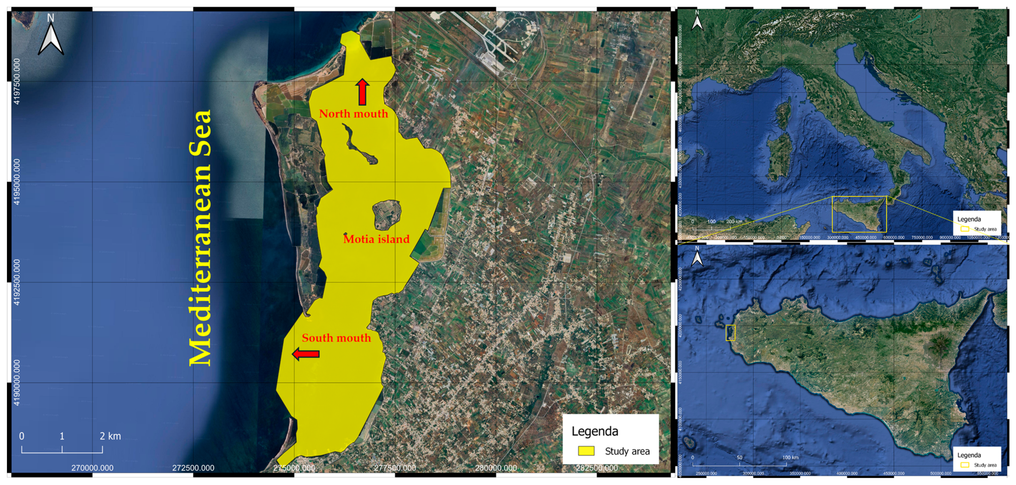
2.1. Study Area

The Stagnone is a coastal lagoon confined by Isola Grande Island, and the main water exchanges with the open sea occur through two different inlet mouths (Figure 1).
The north mouth is 400 m wide, and it is characterized by shallow water, with an average depth of 0.30 m. The south mouth is circa 2900 m wide with a depth of about 1.0–1.50 m.
In the north mouth, water exchange is reduced by the progressive sediment deposition and strong accumulation of dead seagrass leaves coming from the near sea region. This also produces an increase in the characteristic residence time of the particles inside the Stagnone, developing high water temperatures and salinity during the summer. For this reason, the ecological balance of the lagoon is seriously at risk, and a 10 m wide and 1 m deep channel was dredged on the west side of the north mouth inlet to increase water exchange and to allow the transit of small vessels. Because of effects of seasonal freshwater are negligible [4], the hydrodynamic mixing is predominantly influenced by sea-related phenomena and wind.
Inside the lagoon, the mean water depth is less than one metre (circa 0.95 m), with a decreasing depth going northward. From a hydrodynamic point of view, the Stagnone can be divided into two different parts: the southern part (from the south mouth to Motia Island) is characterized by deeper water, and the northern part, on the other hand, is shallower with a water depth lower than 0.90 m and elevated residence times.
In the southern part, the water elevation is strongly dependent on the offshore regions entering from the south mouth [2]. In the northern part, the effects produced by secondary phenomena are dominant, following what was found in [7].
As demonstrated by [2], Posidonia oceanica is the main biotic component in the Stagnone. It covers the central part of the lagoon area with atoll patterns (10–20 m in diameter) and reef formation (1–2 m wide). Where hydrodynamic conditions and sediment composition worsen for P. oceanica, the seagrass meadow is partially replaced by Cymodocea nodosa and Caulerpa prolifera [4].
A bathymetric survey was performed in 1999 and shows very shallow waters in the northern area of the lagoon, with an increasing depth moving southward. A sketch of the bathymetry is reported in Figure 2b, where it is possible to appreciate the deeper water in the southern region and shallower waters in the middle–north area.
The submerged vegetation produces a loss of energy due to plant-induced forcing acting on the fluid, resulting in smaller wave heights [16]. It is important t12o underline, as found by [12,17], that since in the northern part of the lagoon the water is shallower, the relative submergence of the vegetation is higher, inducing a higher damping effect for the hydrodynamic circulation.

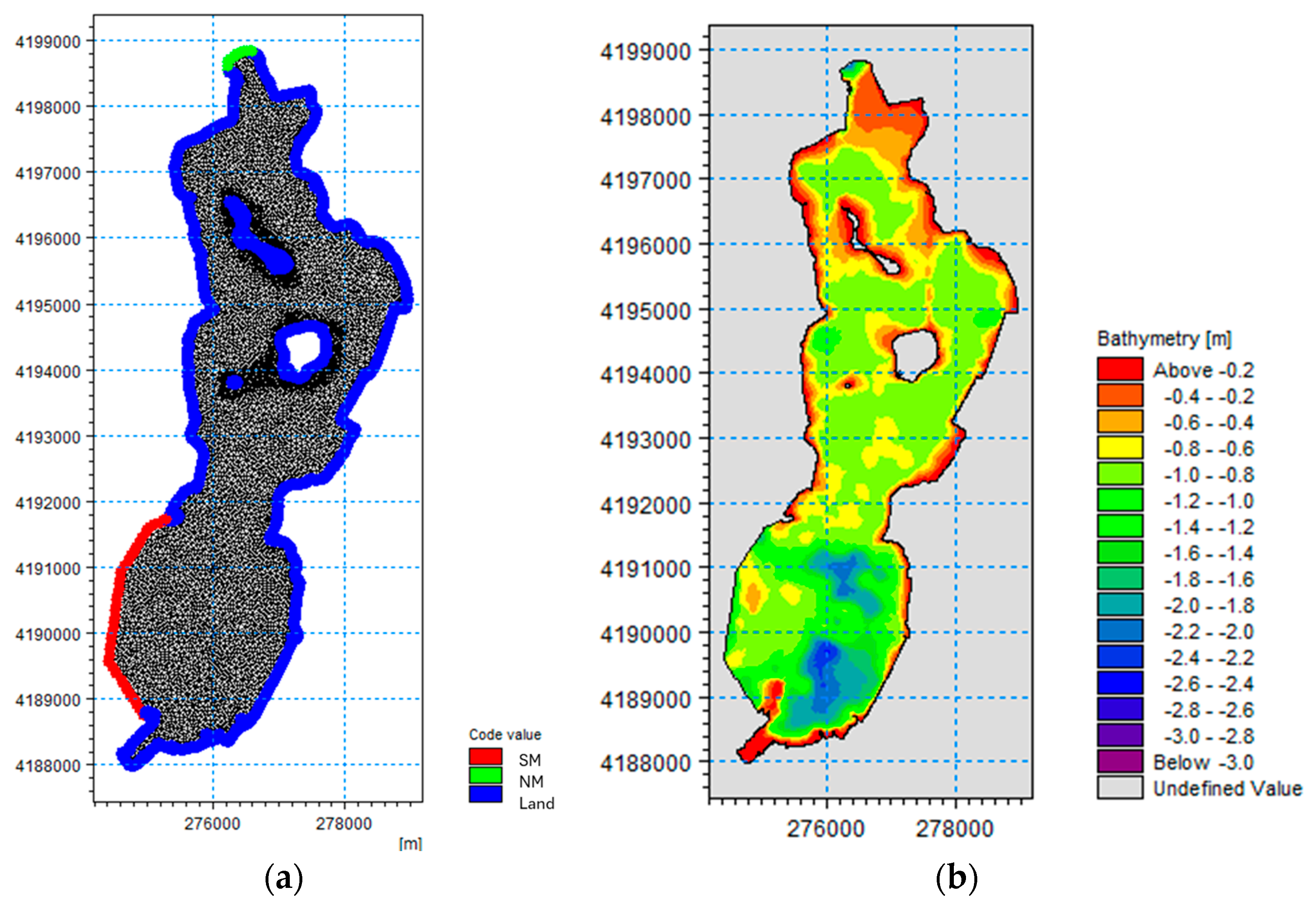
2.2. Numerical Model

As already mentioned, coastal basins such as the Stagnone are mainly characterized by tidal and wind forces. A state-of-the-art 2DH model has been used, simulating the water depth changes and the horizontal velocity components.
The model used is the MIKE 21 Flow Model (MIKE21 HD). This is a hydrodynamic model that is a general numerical modelling system for the simulation of water depths and velocities in coastal areas. The Reynolds-Averaged Navier–Stokes (RANS) and continuity equations are solved, and the model simulates unsteady two-dimensional flow in one-layer (vertically homogeneous) fluids. This module has been applied in a large number of studies related to coastal lagoons [18,19,20]. For further information, refer to the official documentation (DHI suite https://www.mikepoweredbydhi.com, accessed on 5 September 2023).
An unstructured mesh, composed of 15,172 nodes and 25,812 triangular elements, has been created, imposing a finer extent of mesh elements in peculiar lagoon areas such as the inner islands and the northern dredged channel. The element dimensions span from 3000 m2 to 0.1834 m2, representing, respectively, the flatter and more homogeneous zones and the more morphologically complex shallow shores. To avoid numerical inaccuracy, the mesh size has been drastically reduced where local singularity was present.
Two boundary conditions were placed in the north mouth (NM) and in the south mouth (SM), imposing the recorded water depth (Figure 2a).
Figure 2. (a) Unstructured mesh used for the numerical simulations and (b) bathymetry recorded during the 1999 survey.
Water 16 02602 g002
To reach the best set-up, different conditions have been tested. A calibration related to the bed roughness has been conducted to represent the friction induced by the presence of vegetation; for this purpose, the Chezy coefficient has been expressed in terms of the Gauckler–Strickler coefficient Ks. It was possible to attribute a friction coefficient value to represent the presence of Posidonia oceanica, Caulerpa prolifera, and Cymodocea nodosa.
One other calibration parameter was the wind friction factor value f, used to linearize the drag effect of the wind blowing over the water surface. This coefficient is difficult to calculate and depends on the geometry of the water body, the fetch available, and the intensity of the wind itself.
In this case, the wind friction factor was considered independent of wind velocity intensity.
Finally, the last parameter used to calibrate the model is the horizontal eddy viscosity factor, calculated using a constant eddy formulation or the Smagorinsky formulation [21]. The effective shear stresses in the momentum equations contain momentum fluxes due to turbulence and enter the equation through the τ x x   and τ y y variables. This parameter takes into account the damping factors of short-wavelength oscillations and is responsible for representing sub-grid-scale effects. This horizontal viscosity is a function of the partial derivative of flux variation along the x and y directions, like the x ( h τ x x ) term of the following equation, thus being more relevant in those areas where velocity divergence between mesh elements is higher. For deeper information about the numerical solution, it is suggested to consult the MIKE 21 scientific documentation.
In the MIKE21 numerical model, the previous parameters enter in the momentum equilibrium equation, reported below for the x direction.
p t + x ( p 2 h ) + y ( p q h ) + g h ζ x + g p p 2 + q 2 C 2 h 2 1 ρ w [ x ( h τ x x ) + y ( h τ y y ) ] Ω q f W W x + h ρ w x   ( p a ) = 0
where:
  • p a = atmospheric pressure [kg/m/s2];
  • p , q = flux density in the x and y direction, respectively [m3/s/m];
  • g = gravity acceleration [m/s2];
  • h   = water depth [m];
  • ζ = surface elevation [m];
  • C = Chezy resistance [m1/2/s];
  • ρ w = water density [kg/m3];
  • τ x x   ,   τ y y = components of effective shear stress;
  • Ω = Coriolis parameter [s−1];
  • f = wind friction factor;
  • W ,   W x = wind speed and x component [m/s].
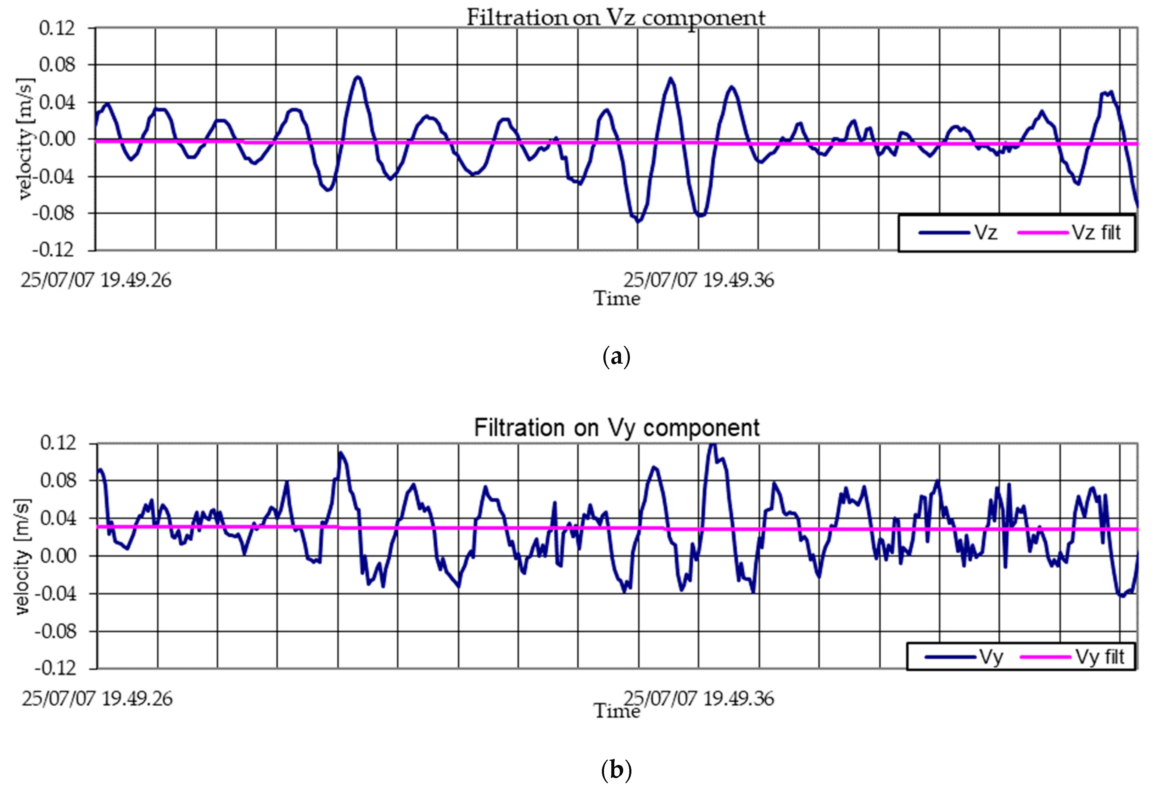
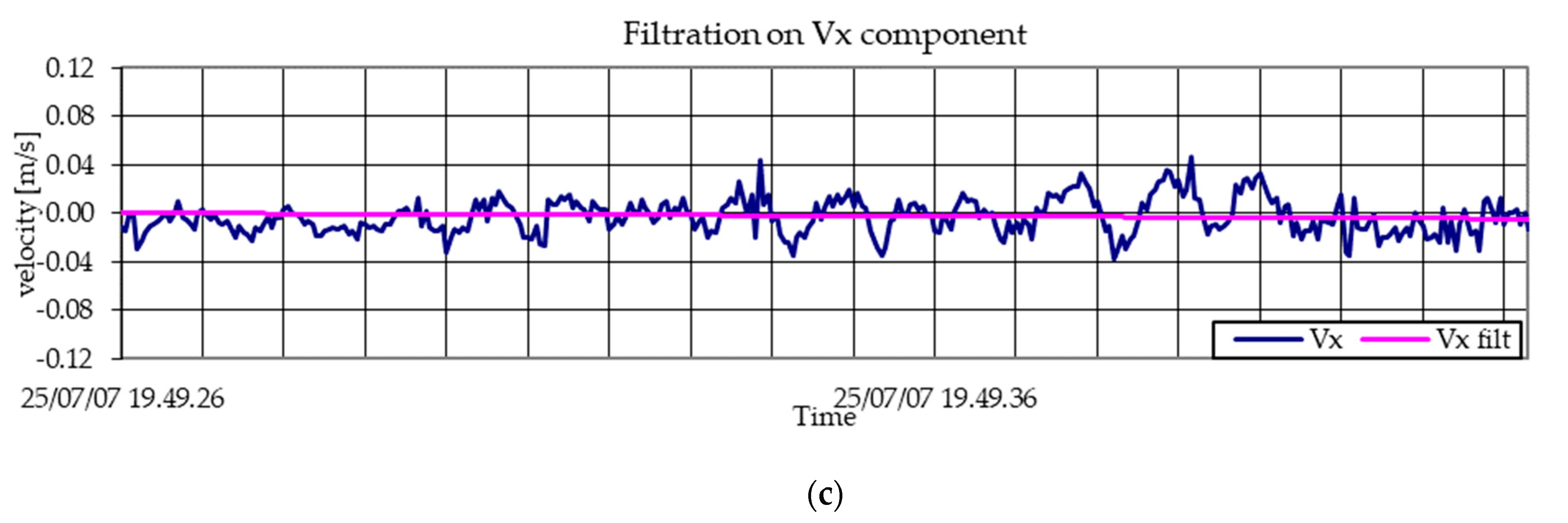
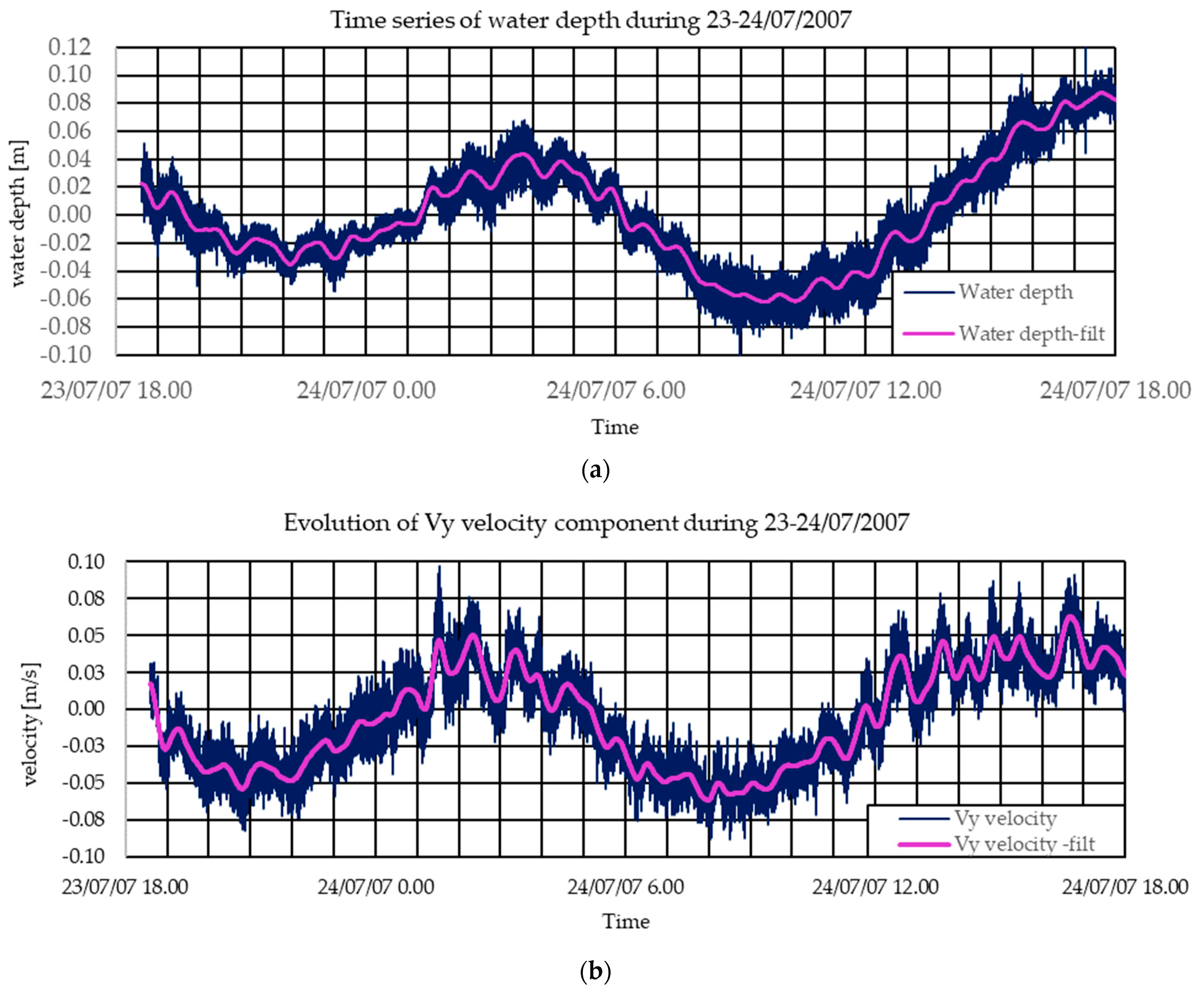
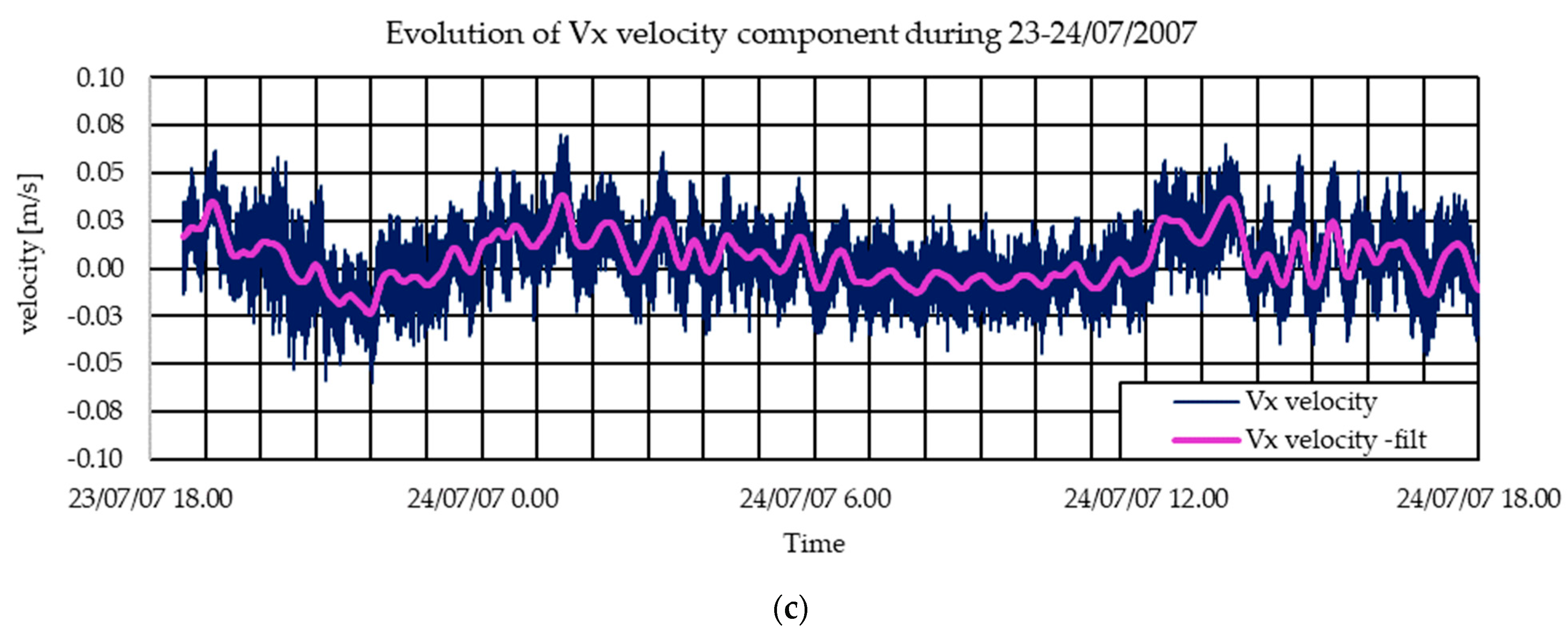
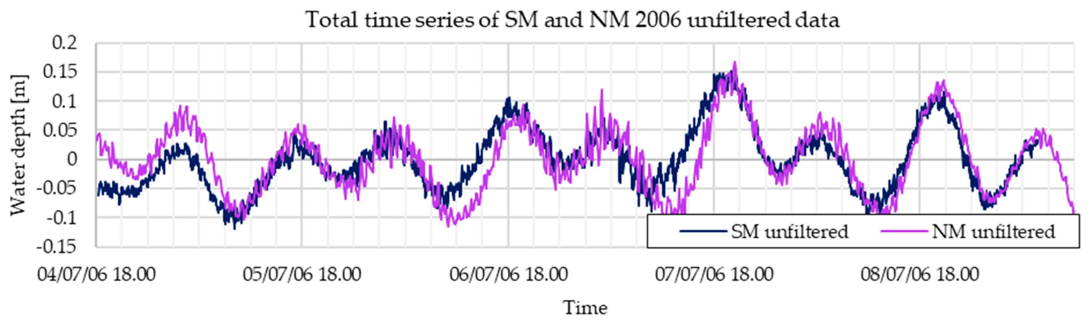
The simulations have been conducted with a timestep of 5 s, using a soft start to avoid a simulation shock caused by the initial condition. In fact, the simulation period starts two days before the recorded data in both cases. The machine in which the simulations were run is equipped with a 12th Gen Intel(R) Core (TM) i7-12700K with a velocity of 3.60 GHz and a RAM of 16.0 GB. The simulation time is about 120 min.
To compare the output generated by the model to the measured values, the Nash–Sutcliffe coefficient of efficiency (NSE) has been used to estimate the goodness of fit of the simulation.
The NSE is calculated by the following formula:
N S E = 1 Σ t = 1 T ( O B S i S I M i ) 2 Σ t = 1 T ( O B S i O B S i ¯ ) 2
where OBS i is the value recorded at the ith timestep, SIM i is the simulated value in the same timestep, and OBS ¯ is the average of the recorded value.
The NSE can vary from 1 to −∞ and reaches values equal to 1 when the model matches the observed value in every timestep considered.
Higher values of NSE, close to 1, mean a better set-up of the model, which indicates the simulation is a better indicator.
To produce the time series comparison, MIKE Zero Time Series Comparator was used, which is a post-processing tool that facilitates the comparison of recorded and simulated time series by computing performance measures and producing relevant comparison plots.
Other statistics like RMSE, R2, and scatter plots can be found in Appendix A. All the analyses were performed with a MATLAB built-in package (https://www.mathworks.com/products/matlab-online.html).

2.3. Field Data

The model has been used referring to two different field campaigns, using different measuring instruments. The first field campaign occurred during the first week of July 2006, and the other one during the last week of July 2007. During both, the free-surface level in the southern mouth (SM) was obtained through a pressure sensor (Valeport 808 EM). The pressure was recorded every 2 min (Table 1). The water elevation at the northern mouth (NM) was registered using a float-operated shaft encoder (Ott Thalimedes), located in a box connected to the dredged channel of the north mouth, as reported in Figure 3. The sea level was measured every minute, while the mean value was recorded every 5 min (Table 1).
The water velocity was measured in three stations inside the lagoon. In the stations Adv and Vec, two ultrasound current meters of Nortek (Adv and Vector) were deployed (Figure 3). By means of these velocimeters, it is possible to acquire the three-dimensional velocity components with a sampling rate of up to 25 Hz. The measured velocity refers to a single point, with a sampling volume diameter of about 10 mm.
The third current meter is the Val (Valeport 808 EM), which is an electromagnetic velocimeter, with a minimum sampling rate of 2 s (0.5 Hz). In the Vector and Valeport, a pressure sensor measures the level oscillation of the free surface.
Velocity measurements were placed at 65% of the mean water depth, counting from the bottom, in order to take into account the influence of the submerged vegetation’s ability to damp the water velocity inside the canopy [22]. To retrieve representative values of the velocity profile in all directions, we suppose that the vertical velocity profile above the canopy follows a logarithmic profile, as found by [23].
The wind stations (Aanderaa Instruments for the 2006 campaign and LSI Lastem for the 2007 one) were both located 3 m above sea level.
The locations of the recording stations deployed during the 2006 and 2007 campaigns are shown in Figure 3.
A short measurement sketch (20 s) by Adv_07 at 20 Hz shows the characteristic orbital motion due to the wind waves [24] (Figure 4). The period of these oscillations is about one second (like the wind waves), and in this temporal frame, the velocity Vy can range from +0.12 m/s to −0.04 m/s (Figure 4b; Vy is positive northward).
In the 2DH numerical model, these sinusoidal velocities are not reproduced since only the averaged velocities are simulated. Then, the recorded oscillations were filtered using a digital low-pass filter (Butterworth filter) to erase the wave-induced velocity effects.
In the 20 s sketch reported in Figure 4b, the filtered velocity Vy was nearly +0.04 m/s. This means that in the Adv_07 station, the mean current flows northward, in accordance with the entering tide in the lagoon from the south mouth.
It is also possible to observe that the component Vx is oscillating around zero during the recording time (Figure 4c) so that the mean flow in the east–west direction is almost insignificant with respect to the Vy mean motion. In addition, the Vz vertical velocities are oscillating around zero (Figure 4a).
Now, we consider the water depth h and the horizontal velocities Vy and Vx recorded for 24 h at the station Vec_07, located near the south mouth, with a frequency of 1 Hz (Figure 5). The variability in the raw data (blue line) is due to the orbital motion of wind waves. Then, a digital filtration of the wind waves is performed (magenta line).
Primarily, a long period of sinusoidal behaviour related to the tide oscillations is clearly recognizable. When the water depth h is decreasing, then the water velocity Vy is negative, i.e., the tide leaves the Stagnone towards the south. When the water depth h is increasing, then the water velocity Vy is positive, i.e., the tide enters the Stagnone from the north.
A secondary phenomenon recorded by the instruments is the seiches, with a period lower than one hour. During a seiche oscillation of the level, the water velocity accelerates and decelerates. In fact, in less than one hour, during a seiche period on 24 July at 02:00, it is possible to appreciate that the filtered velocities Vy, recorded by Vec_07, decelerate from +0.05 m/s to 0.00 m/s, then return to +0.04 m/s (Figure 5b). Seiches are typical lagoon or semi-enclosed basin phenomena. External forces generate a local elevation of the free surface, which is reflected within the basin. Seiches characterize the whole lagoon basin; in fact, they can be observed in all field measurements.
The water depth measured in the first week of July 2006 at the north and south mouths shows first the 12 h period of the tide signal and second the presence of seiches (Figure 6). These unfiltered water levels will be imposed as boundary conditions in the north mouth (NM) and in the south mouth (SM) to force each simulation to introduce a tide-induced effect. In these stations, no velocity data were collected, so only the tidal effect was imposed along the boundary conditions. In fact, these two station were placed in strategic points of the area in order to collect both diurnal and semi-diurnal tidal effects and the peculiar phenomena of the induced seiches. The two mouths are 7 km apart from each other, and the tidal signal is sometimes slightly shifted. The north mouth signal, in fact, appears to be more affected by seiches and strong winds, which induce, respectively, a higher noise along the signal and a more rapid decrease in water depth in correspondence with northward-directed wind. Both boundary conditions are set constant along the boundary as the measurement is considered representative of tide effect along the boundary.
During the 2006 field campaign, wind data were collected at the Anderaa station, placed at 3 m above the mean sea level in the same location as Vec_06, but in 2007, the station used was LSI (as reported in Table 1), and it was placed in correspondence with Adv_07. The wind forcing has been implemented in the model imposing a spatial homogeneous value, with a constant friction factor, as discussed below.

3. Results and Discussion

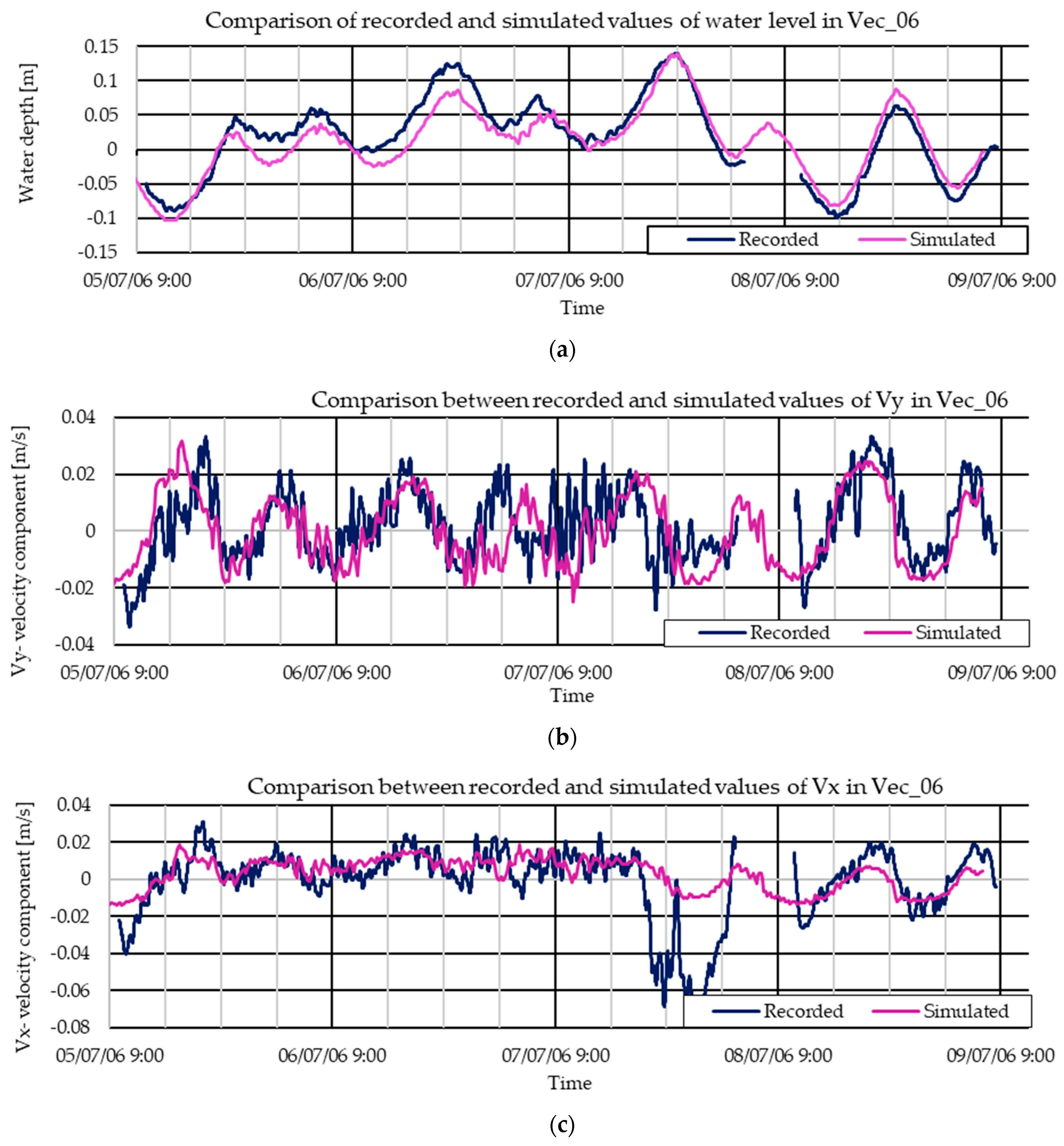
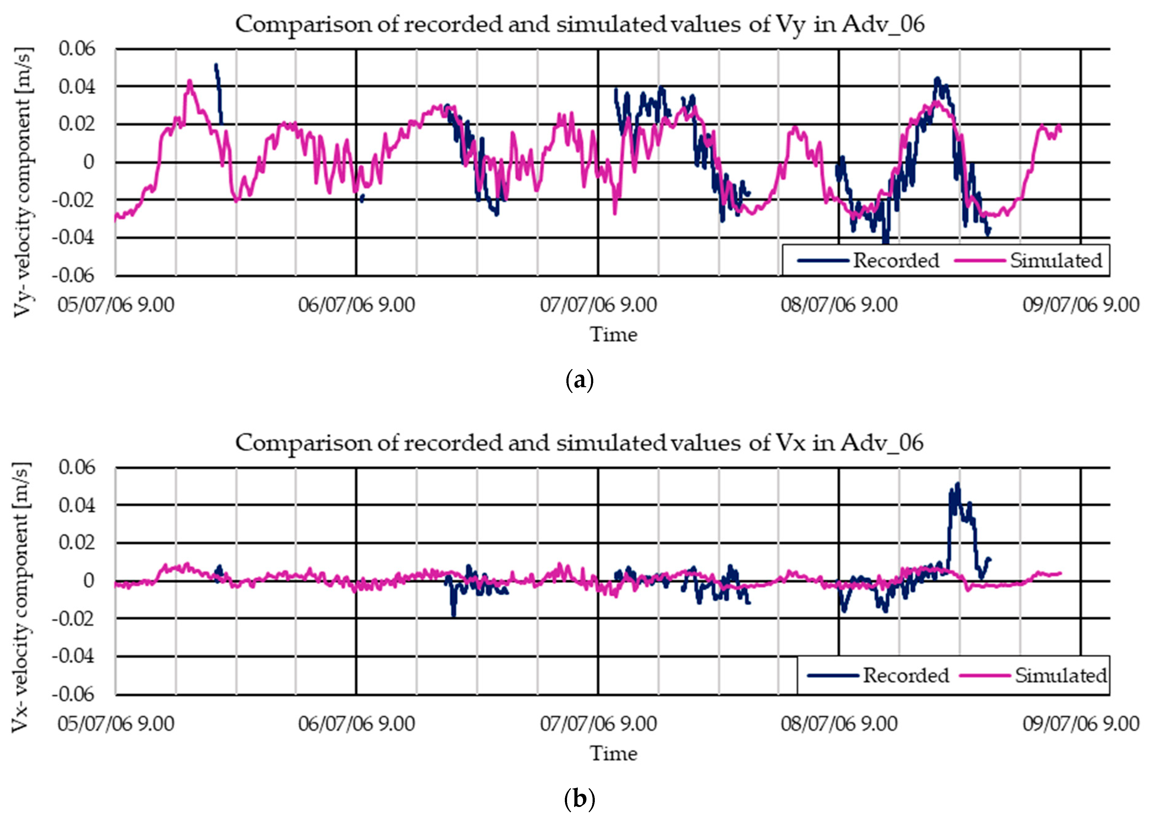
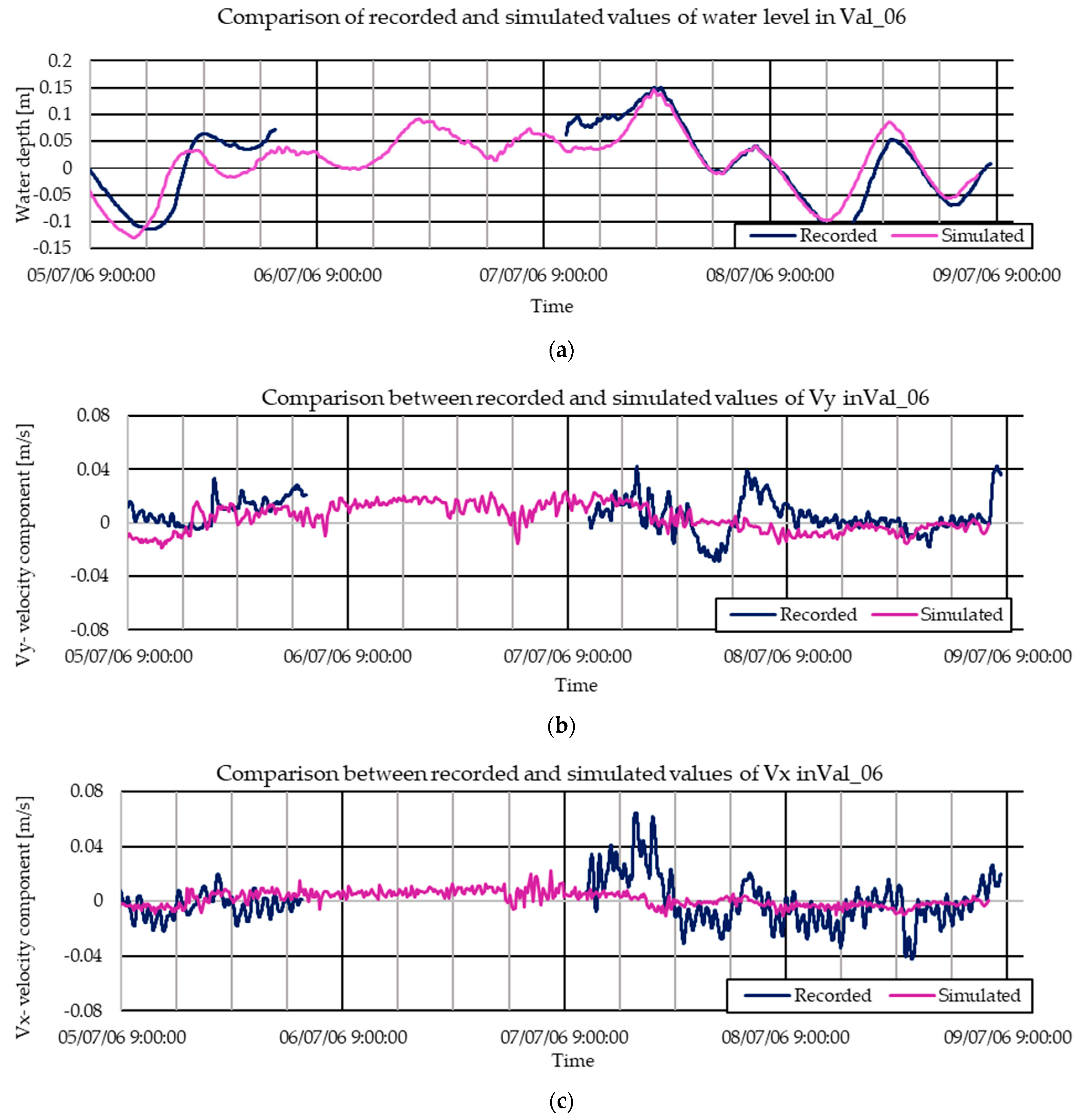
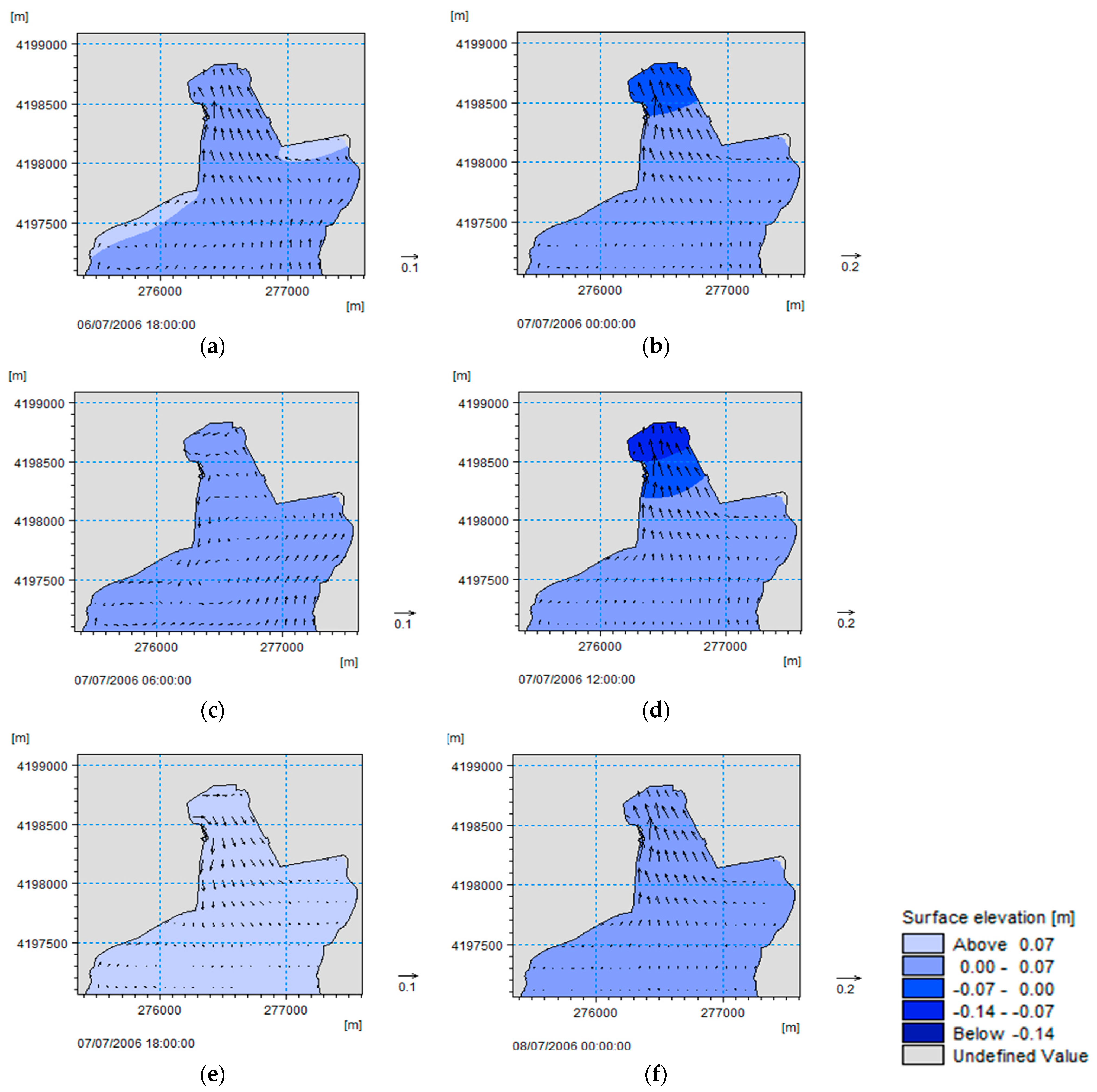
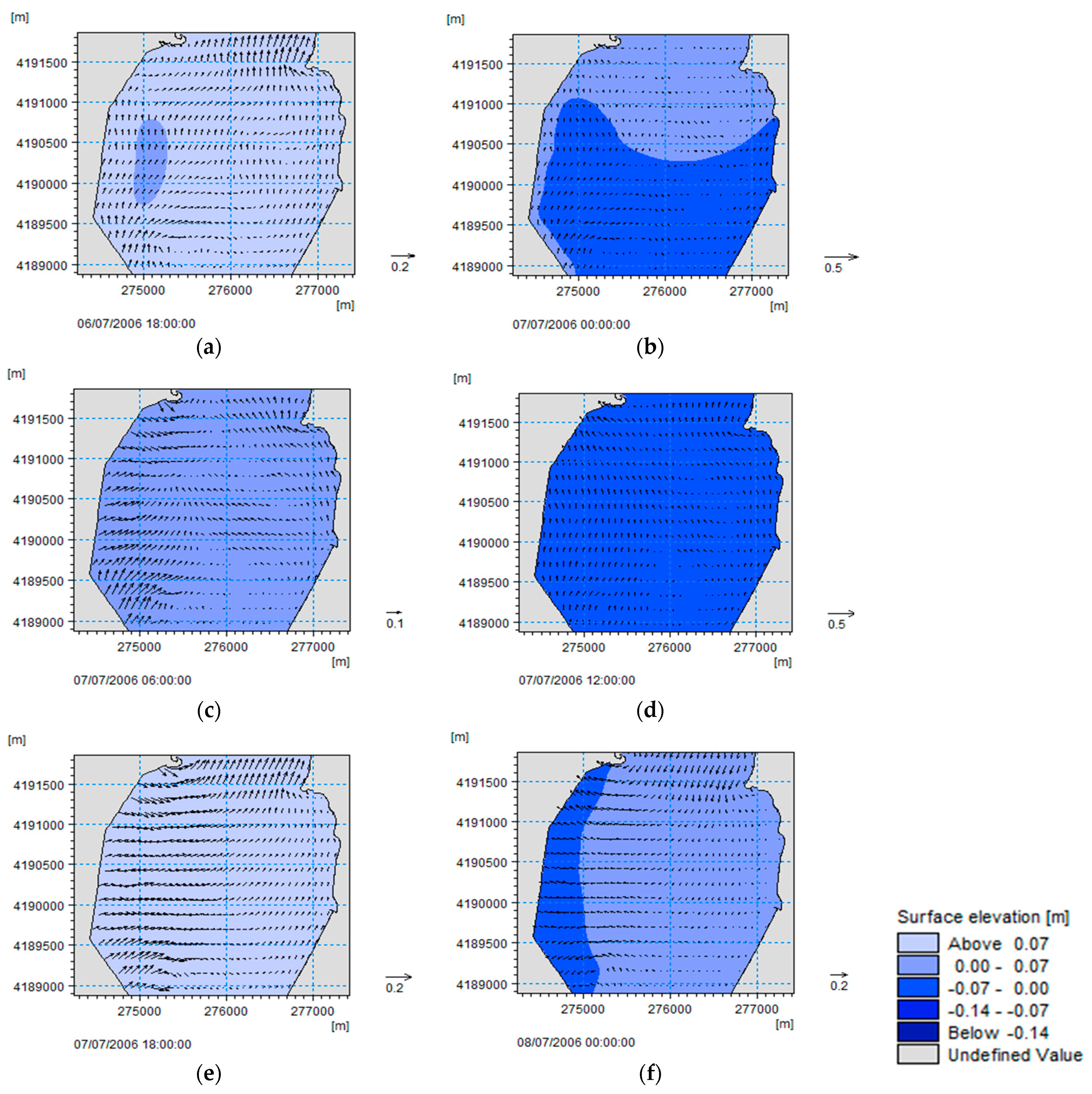
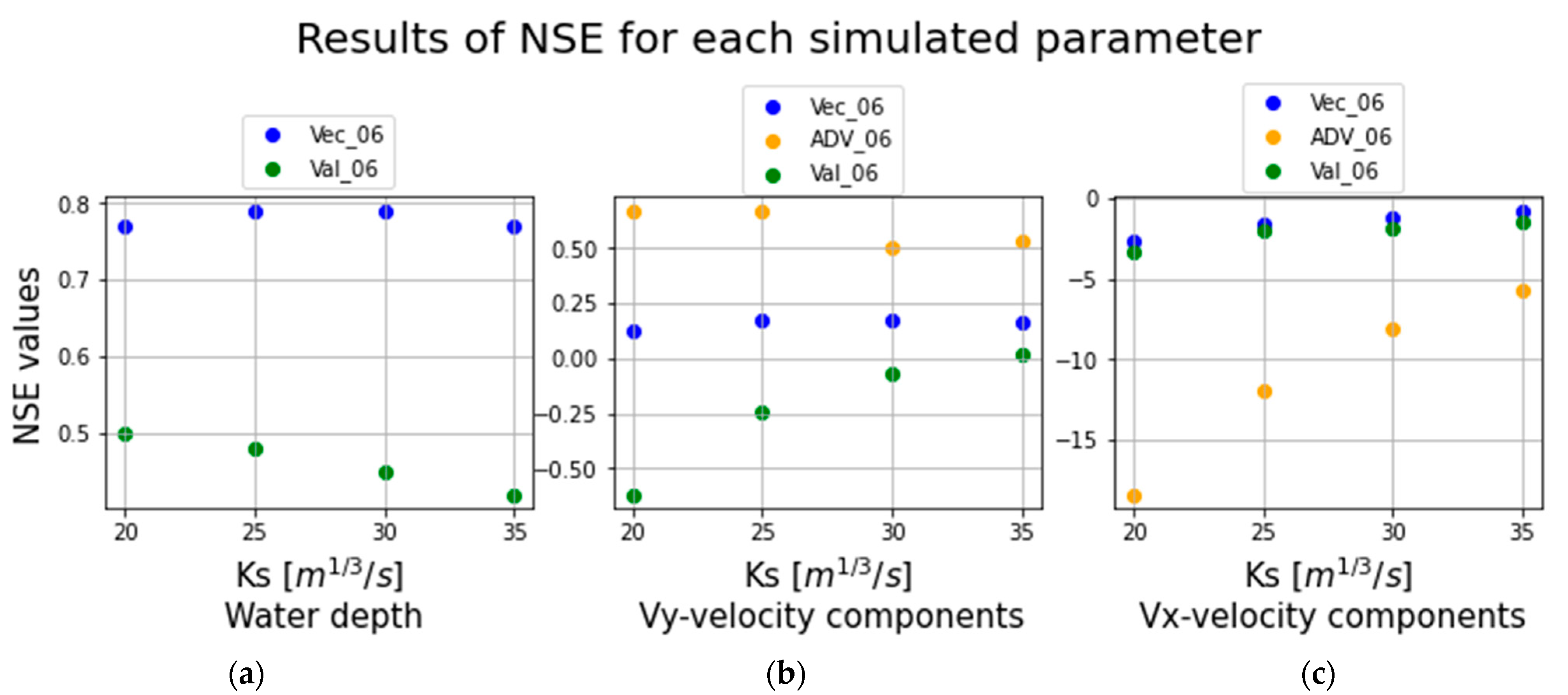
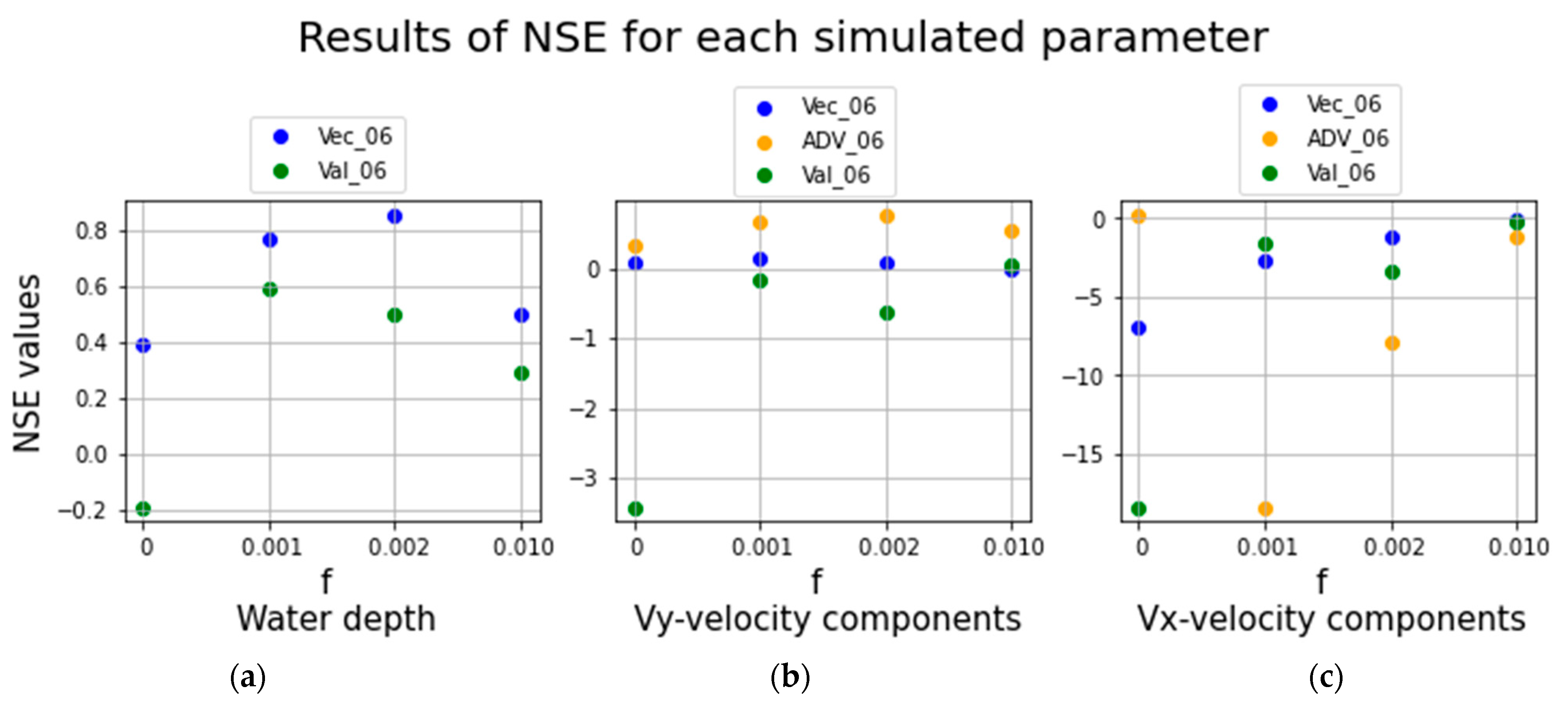
3.1. Calibration with 2006 Data

Initially, the Gauckler–Strickler coefficient Ks = 20 m1/3/s was set as constant in the whole area, and the wind friction factor coefficient was set as f = 0.0010, similarly to the value found by [25], who used f = 0.0014 for W < 10 m/s, and as it was recognized as more reasonable for running the model. The default coefficient suggested by MIKE21 (f = 0.0026) returns values strongly conflicting with the recorded ones. Finally, the effects of the eddy viscosity parameter did not modify the lagoon behaviour when imposed as a constant eddy formulation, starting from ν = 0.0   m 2 s , until values of ν = 1.2 m 2 s . By default, MIKE21 suggests a constant value of ν = 0.002. Furthermore, for eddy viscosity, the Smagorinsky formulation was imposed, with a range of specific k coefficients from k = 0.25 to k = 1.00 following [21], but no change in simulated water level and velocities was detected. It was then decided to neglect the simulation of the eddy viscosity.
The numerical model can reproduce the dominant effects of winds and tides, as can be seen in the following figures where it is possible to appreciate the comparisons between the recorded and the simulated evolution of target variables in all the stations.
In Figure 7, it is possible to compare the evolution of water elevation and the Vy and Vx velocity components recorded in Vec_06.
Starting from the comparisons between recorded and simulated time series for Vec_06, it is possible to appreciate that the general hydrodynamic behaviour of the lagoon is replicated even if some difficulties are present. Although the simulated water depth evolution is in accordance with the recorded ones, the Vy velocity component is sometimes in antiphase with the recorded values, as at midnight of 6 July, when the recorded velocities were northward (positive values), but the simulated ones are southward (negative values) (Figure 7b). The worst agreement was found considering the Vx velocity component, especially during the night of 8 July (Figure 7c). These rates of accordance can be estimated from Appendix A (Table A1), where RMSE and R2 are reported.
Even if Adv_06 had technical problems related to a battery failure during the 2006 campaign, it is possible to appreciate that the general behaviour is replicated, especially for the Vy velocity component (Figure 8a). The Vx component has a bad agreement during the night of 9 July (Figure 8b), when a strong acceleration recorded in the velocities, due to seiches, is not reproduced by the simulation.
Finally, in Figure 9, it is possible to appreciate the evolution of the simulated and recorded water level values, as well as the Vy and Vx velocity components of Val_06, in the northern part of the lagoon. In some moments, the simulated water depth anticipates the recorded one. The range of the simulated Vy is lower with respect to the recorded values. This is particularly the case on the night of 8 July, when the simulated Vy is close zero, but the recorded values reached −0.03 m/s southwards and +0.04 m/s northwards. At 9:00 a.m. of 5 July, the recorded Vy is positive (northward), while the simulated Vy is negative (southward) (Figure 9b).
Looking at global simulation, the hydrodynamic circulation inside the lagoon follows peculiar pattern strongly related to tide and wind variability, as shown in the figure below representing a tidal cycle between 6 and 7 of July 2006. The evolution and the complexity of the hydrodynamic circulation inside the lagoon is represented in Figure 10. The north mouth appears to work as a funnel with strong differences between the two velocity components due to the Venturi effect. It is possible to observe how the outgoing flux corresponds to the ebb tide phase, as on 7 July 2007 at 12:00 p.m. (Figure 10d).
The south mouth is characterized by a higher hydrodynamic circulation and complexity. Wider width and deeper water allow the fluid to develop velocities where there is a combination of the tide and large eddy effects (Figure 11a). Large eddies could be caused by wind blowing and site morphology (Figure 11c). As shown in the north mouth, even in this case, the flux corresponds to the ebb tide phase (Figure 11f).
Comparing the simulations against the recorded data, the NSE parameter is used to compare the prediction capability of different model set-ups. The predictivity capacity is dependent on the differences between the recorded time series and the simulated one. Starting from the comparisons of the simulations showed above, for the two stations Vec_06 and Adv_06 in the centre of the lagoon, it was possible to obtain, in Vec06 for the water depth, a value of NSE = 0.77, and for the Vy and Vx velocity components, respectively, NSE = 0.13 and NSE = −2.63 (Table 2). In Adv_06, we found NSE = 0.67 and NSE = −18.37 for the Vy and Vx velocity components, respectively, considering the longest recording period between the 8th at 08:46 a.m. and the 9th at midnight, as can be seen in Figure 8.
In Val_06, the northernmost station, the obtained values are NSE = 0.50, NSE = −0.62, and NSE = −3.37 for water depth, Vy, and Vx variables, respectively (Table 2). The positive values of NSE for water depth mean that the model acceptably reproduces the water level oscillation. The positive values of NSE for the velocity in the north–south components are acceptable from the south mouth up to the centre of the lagoon. The simulated Vy is not acceptable in the northern part of the lagoon (NSE < 0 in Val_06, Table 2). Finally, the simulated east–west component Vx is not acceptable (NSE < 0 in all the three stations).
To increase the model reliability, different values of bed roughness Ks were tested: from 20 m1/3/s to 35 m1/3/s. The NSE values for the water depth are always positive (0.42 < NSE < 0.79) for the Vec_06 and Val_06 stations (Figure 12a). For the Vy velocity, the NSE is positive (0.13 < NS < 0.67) in the Vec_06 and Adv_06 stations. But in Val_06, the furthest station from the southern mouth, the NSE for the Vy velocity is negative under almost any tested roughness condition, probably because the simulation does not adequately predict the velocities in the northern part of the lagoon (Figure 12b). For the Vx component, the NSE is always negative in the three stations for the different roughness values tested (Figure 12c).
It is possible to underline how the predictive ability of the model varies in different lagoon areas, appearing to be better close to the Vec_06 and Adv_06 location, the stations closer to the south mouth and close to the southern boundary input.
The Val_06 station velocities, referring to the area in the northern part of the lagoon, appears to be the worst described by the model, probably due to the presence of damping effects caused by leafy vegetation.
The lowest NSE values are recorded by the northernmost station, where the ratio between vegetation height and water depth is lower than the southern area. The damping effect of the vegetation in hydrodynamics is well known [26]. The flow over a vegetated bed is characterized by friction velocities depending mainly on the Reynolds number, canopy density, and canopy height [27].
From the comparison of the NSE values for level and velocity, it was possible to figure out the behaviour of the model in response to changes in the bottom roughness. In fact, the simulation with the smallest Gauckler–Strickler coefficients returns, generally, the highest values of NSE. Considering the magnitude of the variation in terms of NSE, a constant Ks equal to 20 m 1 3 s appears to represent the behaviour of the lagoon.
To estimate the influence of wind forces, considering a homogeneous Ks = 20 m 1 3 s , several simulations with different values of the wind friction factor f have been run.
It is possible to observe how the wind is important in the simulations. For example, when f = 0, the NSE’s values for Vy (Figure 13b) remain around zero, showing a poor reliability of the model if wind is neglected. A wind friction coefficient close to f = 0.001–0.002 returns modelled values closer to the recorded ones, as shown on Figure 13.
Different eddy viscosity values were tested, and the Smagorinsky formulation was also tested. But no significant effects are reported in the simulation values due to the changes in the eddy viscosity parameter, showing the negligible effect that this parameter plays in this context, probably because the velocity divergence between mesh element is irrelevant.
In lagoon areas such as the Stagnone, more attention must be given to parameters such as the wind friction factors and the bed roughness.

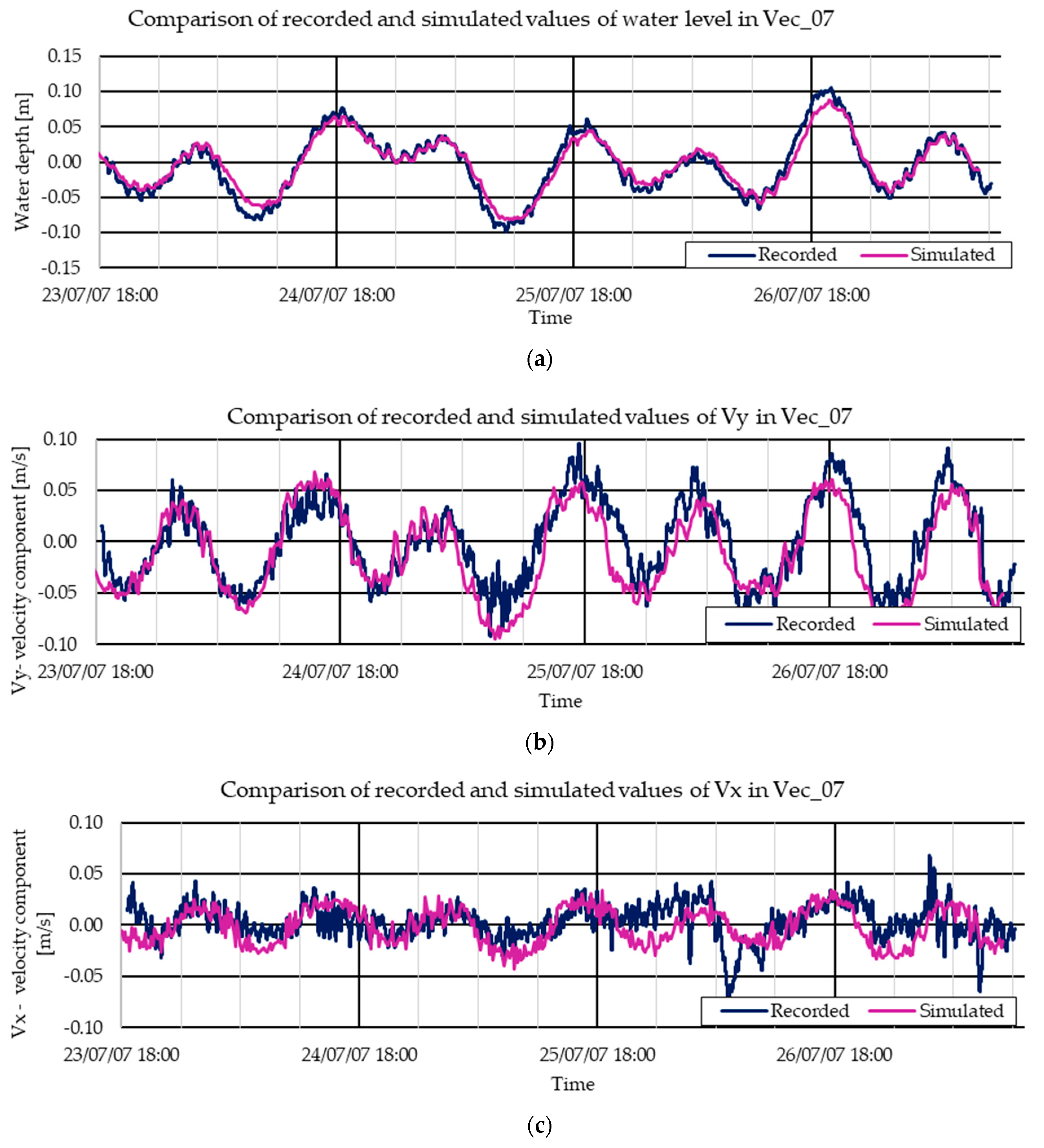
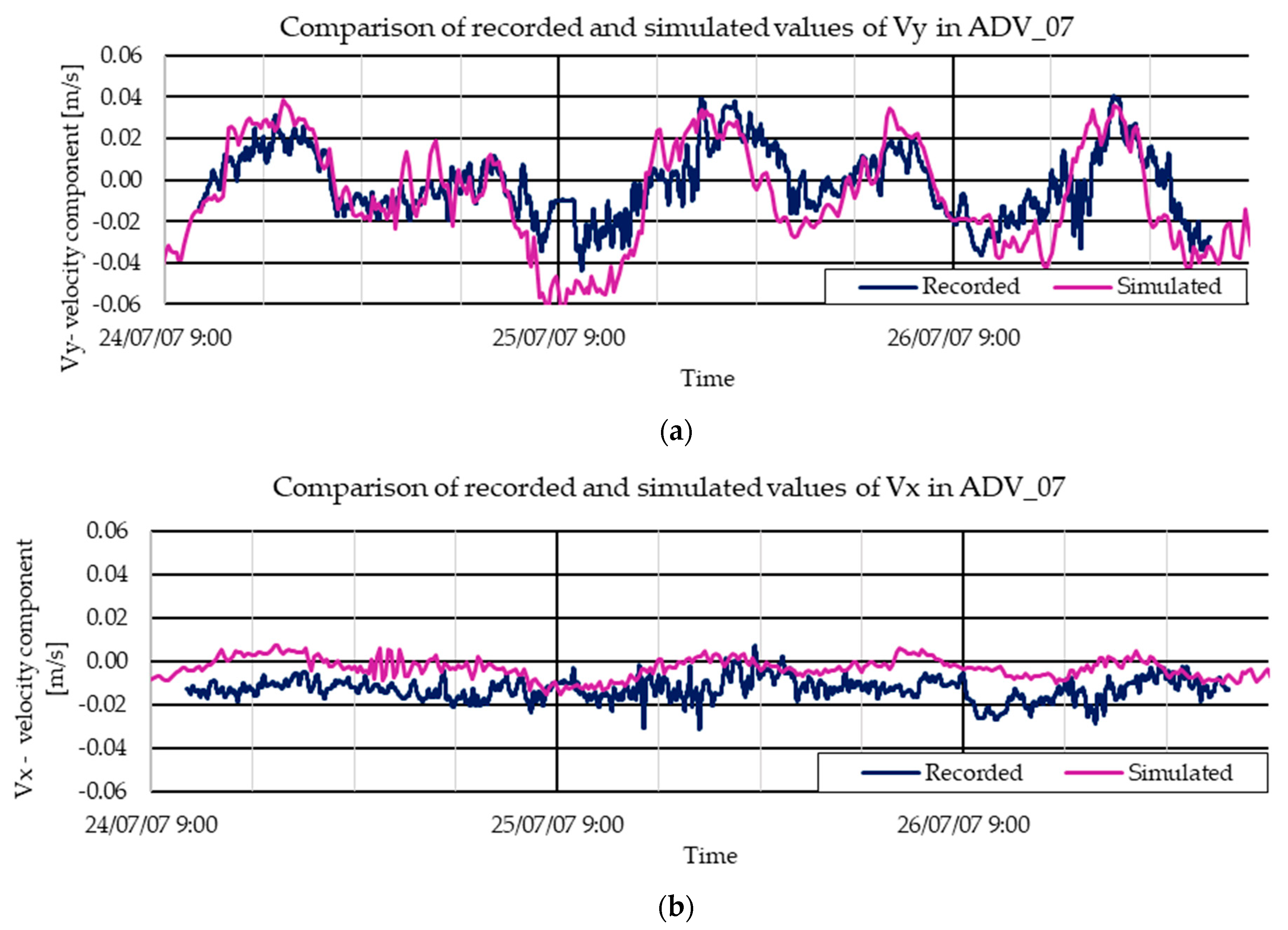
3.2. Validation with 2007 Data

After the calibration with 2006 data, a validation process was conducted for the 2007 campaign. Starting from the optimum set-up model found during the calibration, the simulation of the 2007 field campaign was tested using the following parameters: Strickler Ks = 20 m 1 3 s and wind friction factor f = 0.0020, neglecting the eddy viscosity term.
Again, instrumentation was deployed in the most representative areas of the lagoon, and the following time series show the model attempts replicating the behaviour of the lagoon. Starting from the south side, the times series will be described below.
Starting from Vec_07, the closest station to the south mouth, it is possible to underline a better evolution, with respect to 2006 data, of the water depth and Vy velocities. The results show NSE = 0.92 for water depth and NSE = 0.72 for Vy. The Vx components remain badly simulated, resulting in an NSE = −0.32 for Vx, and the seiches are poorly replicated as well (Figure 14).
Moving to the centre of the lagoon, in the ADV_07 station, there is some agreement between the simulated values of Vy and the recorded values; NSE = 0.50 for Vy. For the Vx component, there is disagreement; the filtered recorded Vx is generally negative, while the simulated values are generally lower than the recorded ones. In fact, NSE = −10.57 (Figure 15). These rates of accordance between recorded and simulated data can also be estimated from Appendix A (Table A1), where RMSE and R2 are reported.
The northernmost measurement was recorded in Val_07, and from the time series reported in Figure 16, it is possible to see how the simulation had some difficulty replicating the considered variables. The simulated water depth anticipates the recorded one; then, the NSE = 0.28 approaches zero. For the Vy velocity component, the simulation fails in replicating the recorded values simulating generally negative velocities and missing the tidal accelerations and decelerations; NSE = −6.27 for Vy. The Vx velocity component is poorly replicated, mismatching all the hydrodynamic phenomena; NSE = −47.21.
Seiches depend on the combination of the intensity and direction of wind blowing, morphology, and the penetration of another lagoon’s external seiches. These phenomena can induce fluid to move even in antiphase with the wind direction, as can be seen in Figure 16, where the recorded and the simulated Vy velocities and wind vector are reported.
At 20:00 on 25 July and at 18:00 on 26 July, the recorded Vy velocity component was about +0.08 m/s, while the simulated one was 7–0.03 m/s; at the same time, the wind was directed southward with a speed of 8 m/s. This is probably because during the day, the tidal movement from the south mouth was predominant over the effect of the wind. The model appears not to replicate this phenomenon, and this affects its predictivity capacity, generating lower values of NSE. It seems that the main effect of the wind is to create wind waves, rather than generating motion in the north–south direction. In fact, when the wind is absent, the unfiltered water level and velocity Vy do not show noise in the signal. Meanwhile, the wind blows the unfiltered water level, and Vy velocity shows the effect of the orbital motion due to the wind wave (Figure 16). The flow in the north–south direction is mainly due to the tidal motion from the south mouth. In this area, the model seems to account greater importance to wind-induced effects to the motion field, underestimating the effect produced by tidal variations.
The comparison between the 2006 and 2007 simulations shows a better model fit with a constant value of bed roughness between Ks = 20 and 25 m 1 3 s , which can be attributed to the high presence of vegetation.
A sensitivity analysis with 2007 data has been conducted to underline the dependence of the bed friction factor. The NSE values for the simulation with a constant value of Ks = 20   m 1 3 s are reported in Table 3, and a general comparison is summarized in Figure 17.
From this analysis, it is possible to figure out how the model’s predictivity capacity decreases in the northern part of the lagoon. In fact, at the northernmost measurement station, the NSE values are lowest, (Val_06 and Val_07) compared with the ADV and Vector located at centre and south of the lagoon. The reason of the lack of model predictivity capacity in the northernmost areas can be attributed to a lower ratio between vegetation height and water depth in the northern area with respect to the southern area. The condition of low submergence produces an additional resistance factor as a function of the leaf height, density, and flexibility of the vegetation species. In fact, where the water depth and vegetation height are comparable (emergent or slightly submerged), as in coastal lagoons, the velocity profile does not follow a logarithmic law at all, showing a low linear increase in the depth occupied by the vegetation and a major increase above the leaf, towards the top [28]. The macro-roughness effects are appreciable even in water depth evolution [29]. This effect is emphasized in the northern area of the Stagnone Lagoon.

4. Conclusions

The aim of this study is to increase the knowledge about hydrodynamic circulation in Mediterranean coastal lagoons like the Stagnone, testing the predictivity capacity of a 2DH model like MIKE21. These types of model work by averaging the vertical velocity along the depth, and, for this reason, using field vertical punctual measurement as a benchmark, the velocity’s NSE cannot be expected to be high. Moreover, focusing on the recorded values of the Vx component of velocity, it is possible to underline how this component is in a range around zero, and this confirms the predominant importance of the velocity’s Vy component.
The sensitivity analysis conducted has been crucial to understanding the lagoon behaviour, since the presence of the vegetation induced a complex estimation of the bed friction factor; in fact, Posidonia oceanica and Cymodocea nodosa leaves induce a particular roughness in the lagoon bed. Moreover, in the northern area, where there is a lower ratio between vegetation height and water depth with respect to the southern area, the vegetation leaves work differently on the hydrodynamics. Several values of roughness coefficient have been tested, establishing the optimum as Ks = 20–25 m 1 3 s for the 2006 field campaign, confirmed by the simulation of the 2007 field campaign. The rate of accordance between recorded and simulated values can be estimated by reading Table A1 in Appendix A, where RMSE and R2 are reported.
The wind friction factor has been also investigated. All the variables show a dependence on the interaction between the air and the water surface; in fact, the simulation without the wind force returns lower NSE values. A general agreement between the simulated and recorded values can be found using a constant value of wind friction factor equal to f = 0.001–0.002. But in the northern area, at different times, the simulated water velocities are directed towards the south, with the wind, while the recorded ones are directed towards the north, with the rising tide from the south mouth.
The eddy viscosity coefficient does not appear to play a valuable role in the hydrodynamic circulation. For the different tested values, there is no appreciable effect on simulated water level and velocities.
Finally, focusing on the variation in the simulated water depth time series, as well as the Vy and Vx velocity components, it is necessary to underline that the model reproduces the seiches phenomena with difficulty.
In the northern areas, the hydrodynamism of the Stagnone Lagoon is poorly described by the model, and the wind effect is overestimated. Due to the presence of relative high vegetation in the northern area, the motion field is strongly dominated by tides as registered by in situ data. The presence of vegetation in the form of long leaves induces a strong damping effect that cannot be explicated by a common bed roughness coefficient. Nevertheless, the model produces more reliable values in areas closer to the south mouth, as the NSE for water depth and the Vy velocity component suggest. In the southern area, the 2DH model looks more capable of replicating the variability in the water depth and water velocity. Moving northward, the model predictivity becomes more difficult. This implies that all the NSE values are higher when they refer to stations deployed closer to the south mouth.
The Vx velocity component looks poorly replicated, in all cases returning NSE not acceptable, always with negative values.
This study shows how the lagoon circulation is affected by some problems and the dependence on tide and wind regime. Finally, seiches also play a key role in the lagoon circulation, as well as more complex bed roughness effects.
The Stagnone Lagoon is a vulnerable environment with morphological complexity; the circulation is dominated by external forces recorded in two different field campaigns. The global behaviour has been replicated by the MIKE 21 hydrodynamic model with an unstructured mesh, showing the strong dependence of Mediterranean lagoons on the wind, tide, and the inducted seiches forces. A possible improvement could be the implementation of different roughness values, considering higher values of energy loss where the submergence is lower, and vegetation leaves are higher. This could be coupled with a high-definition vegetation map detected, for example, by remote sensors and UAVs. Implementing a “roughness map” could be a valuable improvement that could allow the model to replicate the hydrodynamic circulation in the northern area. Moreover, the 2DH model showed low precision in representing the hydrodynamics induced by local morphology in very shallow water, and this is probably due to a bathymetric accuracy and mesh resolution in shore regions. In fact, the NSE related to the Vx velocity component is expected to increase with more domain morphological details.

Author Contributions

Conceptualization, G.C.; Methodology, G.C.; Software, E.I.; Validation, G.C.; Formal analysis, E.I.; Investigation, C.N.; Resources, G.C.; Data curation, C.N.; Writing—original draft, E.I.; Writing—review & editing, C.N.; Supervision, G.C.; Funding acquisition, G.C. All authors have read and agreed to the published version of the manuscript.

Funding

This work has been supported and funded by the project PO FESR 2014–2020, ASSE 6, Azione 6.5.1, for interventions related to Riserva Naturale Orientata “Isole dello Stagnone di Marsala”, in particular “Interventi finalizzati al Recupero delle condizioni ambientali del bacino dello StagNone di MArsala: applicazioni operative ed elaborazione di SCEnari (RINASCE)”.

Data Availability Statement

Data is contained within the article. Further data are available under request.

Acknowledgments

The authors would like to thank Józsa János and Krámer Tamás from Budapest University of Technology and Economy (BUTE University) for their contribution during the field campaigns.

Conflicts of Interest

The authors declare that the research was conducted in the absence of any commercial or financial relationships that could be construed as a potential conflict of interest.

Appendix A

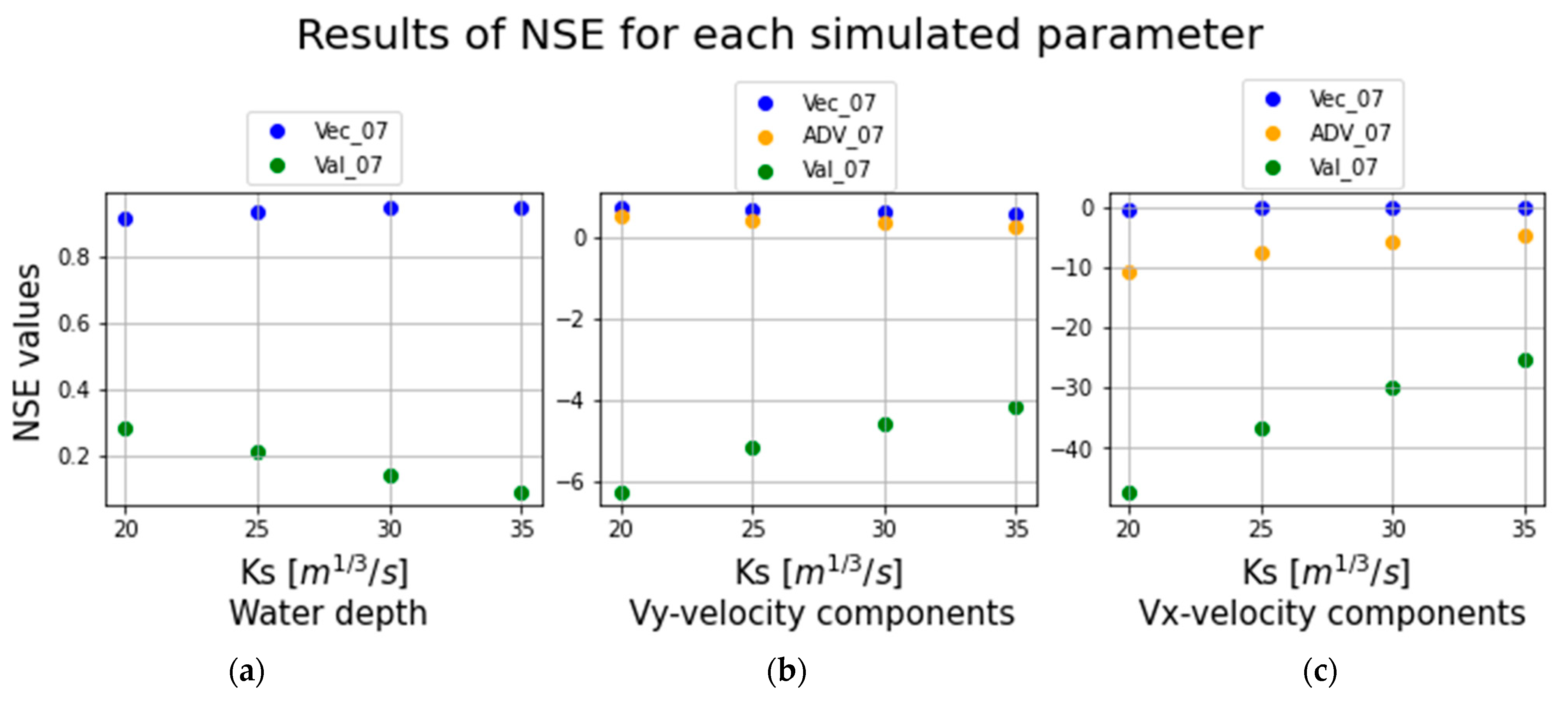
Statistics of 2006 and 2007 Simulation Efficiency

During the calibration and validation processes, different statistics have been calculated in order to track the efficiency of the simulation modelling.
In Table A1, all the statistics are reported, showing the efficiency of the simulations.
Table A1. Statistics of all variables in all simulations conduced against recorded values.
Water LevelVx Velocity ComponentVy Velocity Component
StationRMSER2SIRMSER2SIRMSER2SI
Vec_060.020.881.010.010.39−6.260.010.355.07
Val_060.030.74−3048.960.000.09−2.220.010.071.77
Adv_06---0.000.100.630.020.00−1.78
Adv_07---0.000.02−0.350.020.59−7.69
Val_070.030.57−129.000.000.04−0.340.020.001.25
Vec_070.010.96−1.640.020.214.90.020.77−10.64
Below, in Figure A1, are reported all the scatter plots showing the simulated data against the recorded data on the recording stations. The plots reported are related to the simulations with a positive and reasonable NSE value.
Figure A1. Scatter plots of the recorded and simulated values. All the water (a,d,e,h) level graphs look return an agreement between the variables, even if in both years simulated values of Valeport station returned a sort of delay effect (d,h). Is possible to appreciate the increasing NSE value from Vec_06 to Vec_07 (b,f). The agreement of Vy velocity component looks high scattered (c). The Vy velocity component looks better in 2007 (f,g) than in 2006 (b,c).
Water 16 02602 g0a1aWater 16 02602 g0a1b

References

  1. Inácio, M.; Barboza, F.R.; Villoslada, M. The Protection of Coastal Lagoons as a Nature-Based Solution to Mitigate Coastal Floods. Curr. Opin. Environ. Sci. Health 2023, 34, 100491. [Google Scholar] [CrossRef]
  2. La Loggia, G.; Calvo, S.; Ciraolo, G.; Mazzola, A.; Pirrotta, M.; Sarà, G.; Tomasello, A.; Vizzini, S. Influence of Hydrodynamic Conditions on the Production and Fate of Posidonia oceanica in a Semi-Enclosed Shallow Basin (Stagnone Di Marsala, Western Sicily). Chem. Ecol. 2004, 20, 183–201. [Google Scholar] [CrossRef]
  3. Paugam, C.; Sous, D.; Rey, V.; Meulé, S.; Faure, V.; Boutron, O.; Luna-Laurent, E.; Migne, E. Wind Tides and Surface Friction Coefficient in Semi-Enclosed Shallow Lagoons. Estuar. Coast. Shelf Sci. 2021, 257, 107406. [Google Scholar] [CrossRef]
  4. Mancuso, F.P.; Bernardeau-Esteller, J.; Spinelli, M.; Sarà, G.; Ruiz, J.M.; Calvo, S.; Tomasello, A. Life on the Edge: Adaptations of Posidonia oceanica to Hypersaline Conditions in a Mediterranean Lagoon System. Environ. Exp. Bot. 2023, 210, 105320. [Google Scholar] [CrossRef]
  5. Pascolo, S.; Petti, M.; Bosa, S. On the Wave Bottom Shear Stress in Shallow Depths: The Role of Wave Period and Bed Roughness. Water 2018, 10, 1348. [Google Scholar] [CrossRef]
  6. Petti, M.; Bosa, S.; Pascolo, S.; Uliana, E. An Integrated Approach to Study the Morphodynamics of the Lignano Tidal Inlet. J. Mar. Sci. Eng. 2020, 8, 77. [Google Scholar] [CrossRef]
  7. Pavlova, A.; Myslenkov, S.; Arkhipkin, V.; Surkova, G. Storm Surges and Extreme Wind Waves in the Caspian Sea in the Present and Future Climate. Civ. Eng. J. 2022, 8, 2353–2377. [Google Scholar] [CrossRef]
  8. Simantiris, N.; Avlonitis, M. Effects of Future Climate Conditions on the Zooplankton of a Mediterranean Coastal Lagoon. Estuar. Coast. Shelf Sci. 2023, 282, 108231. [Google Scholar] [CrossRef]
  9. Larroudé, P.; Doua, M. Comparison of Sediment Transport Formulae with Monthly 2DH Simulation on a Sandy Beach and on a Beach with Noneroded Sea Bed Zone. In Proceedings of the Littoral 2010—Adapting to Global Change at the Coast: Leadership, Innovation, and Investment, London, UK, 21–23 September 2010; EDP Sciences: London, UK, 2011; p. 12006. [Google Scholar]
  10. Ondiviela, B.; Losada, I.J.; Lara, J.L.; Maza, M.; Galván, C.; Bouma, T.J.; Van Belzen, J. The Role of Seagrasses in Coastal Protection in a Changing Climate. Coast. Eng. 2014, 87, 158–168. [Google Scholar] [CrossRef]
  11. Cavallaro, L.; Lo Re, C.; Paratore, G.; Viviano, A.; Foti, E. Response of Posidonia oceanica to Wave Motion in Shallow-Waters-Preliminary Experimental Results. Coast. Eng. Proc. 2011, 32, 49. [Google Scholar] [CrossRef]
  12. Leonardi, N.; Carnacina, I.; Donatelli, C.; Ganju, N.K.; Plater, A.J.; Schuerch, M.; Temmerman, S. Dynamic Interactions between Coastal Storms and Salt Marshes: A Review. Geomorphology 2018, 301, 92–107. [Google Scholar] [CrossRef]
  13. Mahapatro, D.; Panigrahy, R.C.; Panda, S. Coastal Lagoon: Present Status and Future Challenges. Int. J. Mar. Sci. 2013, 3, 178–186. [Google Scholar] [CrossRef]
  14. Mulhern, J.S.; Johnson, C.L.; Martin, J.M. Is Barrier Island Morphology a Function of Tidal and Wave Regime? Mar. Geol. 2017, 387, 74–84. [Google Scholar] [CrossRef]
  15. Li, X.; Huang, M.; Wang, R. Numerical Simulation of Donghu Lake Hydrodynamics and Water Quality Based on Remote Sensing and MIKE 21. ISPRS Int. J. Geo-Inf. 2020, 9, 94. [Google Scholar] [CrossRef]
  16. Pillai, U.P.A.; Pinardi, N.; Alessandri, J.; Federico, I.; Causio, S.; Unguendoli, S.; Valentini, A.; Staneva, J. A Digital Twin Modelling Framework for the Assessment of Seagrass Nature Based Solutions against Storm Surges. Sci. Total Environ. 2022, 847, 157603. [Google Scholar] [CrossRef]
  17. Jacob, B.; Dolch, T.; Wurpts, A.; Staneva, J. Evaluation of Seagrass as a Nature-Based Solution for Coastal Protection in the German Wadden Sea. Ocean Dyn. 2023, 73, 699–727. [Google Scholar] [CrossRef]
  18. Simonetti, I.; Cappietti, L. Influence of Inlets Morphology and Forcing Mechanisms on Water Exchange between Coastal Basins and the Sea: A Hindcast Study for a Mediterranean Lagoon. J. Mar. Sci. Eng. 2022, 10, 1929. [Google Scholar] [CrossRef]
  19. Schoen, J.H.; Stretch, D.D.; Tirok, K. Wind-Driven Circulation Patterns in a Shallow Estuarine Lake: St Lucia, South Africa. Estuar. Coast. Shelf Sci. 2014, 146, 49–59. [Google Scholar] [CrossRef]
  20. Fourniotis, N.T.; Leftheriotis, G.A.; Horsch, G.M. Towards Enhancing Tidally-Induced Water Renewal in Coastal Lagoons. Environ. Fluid Mech. 2021, 21, 343–360. [Google Scholar] [CrossRef]
  21. Smagorinsky, J. General Circulation Experiments with the Primitive Equations: I. The Basic Experiment. Mon. Weather Rev. 1963, 91, 99–164. [Google Scholar] [CrossRef]
  22. Ciraolo, G.; Ferreri, G.B.; Loggia, G.L. Flow Resistance of Posidonia oceanica in Shallow Water. J. Hydraul. Res. 2006, 44, 189–202. [Google Scholar] [CrossRef]
  23. Nepf, H.M. Hydrodynamics of Vegetated Channels. J. Hydraul. Res. 2012, 50, 262–279. [Google Scholar] [CrossRef]
  24. Kundu, P.K.; Cohen, I.M. Fluid Mechanics, 4th ed.; Elsevier: Amsterdam, The Netherlands, 2008; ISBN 978-0-12-381399-2. [Google Scholar]
  25. Niedda, M.; Greppi, M. Tidal, Seiche and Wind Dynamics in a Small Lagoon in the Mediterranean Sea. Estuar. Coast. Shelf Sci. 2007, 74, 21–30. [Google Scholar] [CrossRef]
  26. Kobayashi, N.; Raichle, A.W.; Asano, T. Wave Attenuation by Vegetation. J. Waterw. Port Coast. Ocean Eng. 1993, 119, 30–48. [Google Scholar] [CrossRef]
  27. Etminan, V.; Ghisalberti, M.; Lowe, R.J. Predicting Bed Shear Stresses in Vegetated Channels. Water Resour. Res. 2018, 54, 9187–9206. [Google Scholar] [CrossRef]
  28. Neumeier, U.; Ciavola, P. Flow Resistance and Associated Sedimentary Processes in a Spartina Maritima Salt-Marsh. J. Coast. Res. 2004, 202, 435–447. [Google Scholar] [CrossRef]
  29. Sambe, A.N.; Sous, D.; Golay, F.; Fraunié, P.; Marcer, R. Numerical Wave Breaking with Macro-Roughness. Eur. J. Mech.-BFluids 2011, 30, 577–588. [Google Scholar] [CrossRef]
Figure 1. Study area.
Water 16 02602 g001
Figure 3. Localization scheme during the 2006 and 2007 field campaigns. Colours indicate the instrument type.
Water 16 02602 g003
Figure 4. Comparison between filtered and raw signals in vertical (a), northward (b), and eastward (c) velocity components of ADV_07 (20 s sketch).
Water 16 02602 g004aWater 16 02602 g004b
Figure 5. Water depth (a) and horizontal velocities northward and eastward, (b) and (c) respectively, recorded in 24 h at 1 Hz by Vec_07.
Water 16 02602 g005aWater 16 02602 g005b
Figure 6. Evolution of water levels recorded in both mouths.
Water 16 02602 g006
Figure 7. Decoupling of recorded and simulated data on Vec_06, related to water depth (a) and horizontal velocities northward and eastward, (b) and (c) respectively.
Water 16 02602 g007
Figure 8. Behaviour of the Vy and Vx velocity components recorded and simulated in Adv_06, related to horizontal velocities northward and eastward, (a) and (b) respectively.
Water 16 02602 g008
Figure 9. Behaviour of simulated variables against the recorded data of Val_06, related to water depth (a) and horizontal velocities northward and eastward, (b) and (c) respectively.
Water 16 02602 g009
Figure 10. Graphical maps of hydrodynamic circulation. A whole tidal cycle is reported. A strong Venturi effect can be observed in when the flow is outgoing (a,b,d), caused by the falling tide. A modest eddy is simulated in (c). Is also possible to appreciate (df) the tide evolution with 6 h period.
Water 16 02602 g010
Figure 11. Hydrodynamic circulation in the lagoon’s southern region. Is possible to appreciate how the circulation follows the tides (a,c,f). Lower hydrodynamism is simulated in the coastal part of the lagoon (b,d). Is possible to appreciate the 6 h tide evolution (e,f).
Water 16 02602 g011
Figure 12. NSE values obtained by the comparison of Vec_06 (a), Adv_06 (b), Val_06 (c), and simulated ones, depending on bed roughness. All the Ks values are in m1/3/s.
Water 16 02602 g012
Figure 13. NSE values obtained by the comparison of Vec_06 (a), Adv_06 (b), and Val_06 (c) recorded values and simulated ones, depending on the friction factor f.
Water 16 02602 g013
Figure 14. Behaviour of simulated variables (water level, Vy, and Vx velocity components, respectively, in (ac)) against the recorded data of Vec_07.
Water 16 02602 g014
Figure 15. Behaviour of the Vy and Vx velocity components recorded and simulated in Adv_07, related to horizontal velocities northward and eastward, (a) and (b) respectively.
Water 16 02602 g015
Figure 16. Behaviour of simulated variables (water level, Vy, and Vx velocity components, respectively, in (ac)) against the recorded data of Val_07. In (d), the evolution of the wind blowing during 2007 campaign is reported.
Water 16 02602 g016
Figure 17. NSE values obtained by the comparison of Vec_07 (a), Adv_07 (b), Val_07 (c), and simulated ones, depending on bed roughness. All the Ks values are in m1/3/s.
Water 16 02602 g017
Table 1. Instruments characteristics.
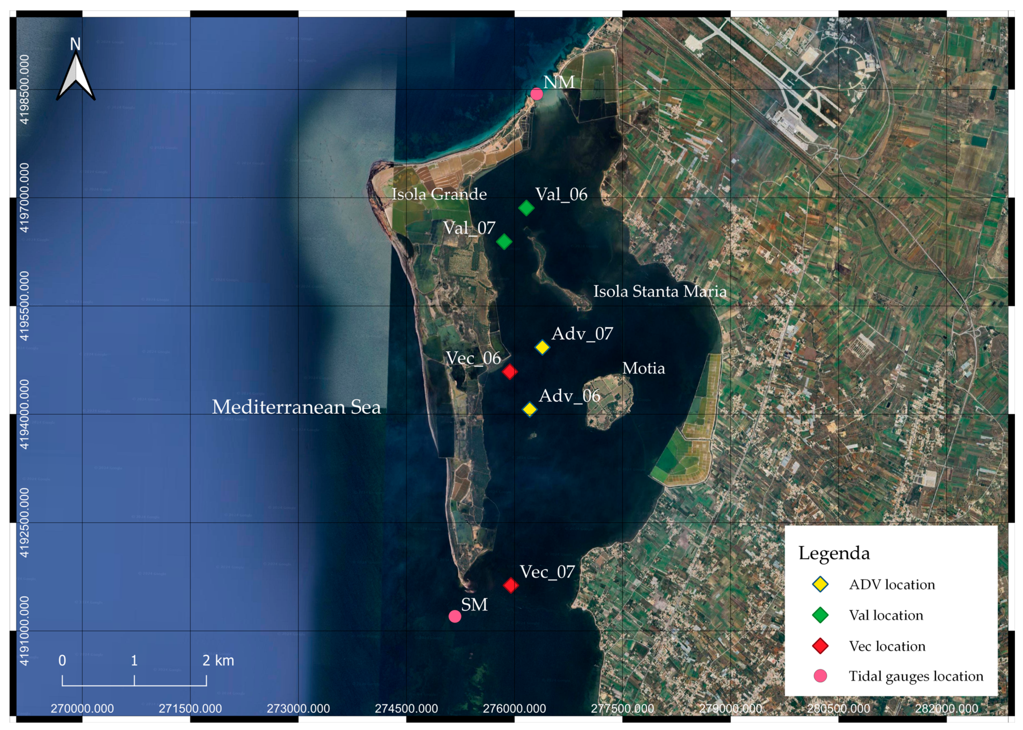
Instruments Characteristics and Acquiring Period
StationInstrumentMeasurePeriod (s)Mean Water Depth (m)Starting TimeEnding Time
South Mouth (SM)Valeport 808 EMPressure1200.6004/07/2006 4:17
23/07/2007 17:54
09/07/2006 7:45
27/07/2007 12:12
Vec 06Vector

Aanderaa
Pressure
Velocity
Wind
60
60
60
1.3005/07/2006 10:0509/07/2006 7:00
Adv 06Nortek ADVVelocity51.2508/07/2006 8:4309/07/2006 00:00
Val 06Valeport 808 EMPressure
Velocity
20
20
1.2504/07/2006 14:4509/07/2006 8:22
North Mouth (NM)Ott ThalimedesLevel3000.60Always recording
Vec 07Vector Pressure
Velocity
10
10
1.5023/07/2007 18:3527/07/2007 11:00
Adv 07Nortek ADV
LSI Lastem
Velocity
Wind
10
5
1.3024/07/2007 11:0427/07/2007 00:41
Val 07Valeport 808 EMPressure
Velocity
20
20
1.0024/07/2007 08:1627/07/2007 10:19
Table 2. Summary of the NSE value for the simulation with Ks = 20 m1/3/s, reproducing the 2006 campaign.
NSEh—DepthVy VelocityVx Velocity
Vec_060.770.13−2.63
Adv_06 0.67−18.37
Val_060.50−0.62−3.37
Table 3. Summary of the NSE value for the simulation with Ks = 20 m1/3/s, reproducing the 2007 campaign.
NSEh—DepthVy VelocityVx Velocity
Vec_070.920.72−0.32
Adv_07 0.50−10.57
Val_070.28−6.27−47.21
Disclaimer/Publisher’s Note: The statements, opinions and data contained in all publications are solely those of the individual author(s) and contributor(s) and not of MDPI and/or the editor(s). MDPI and/or the editor(s) disclaim responsibility for any injury to people or property resulting from any ideas, methods, instructions or products referred to in the content.

