Article

Increased Sensitivity and Accelerated Response of Vegetation to Water Variability in China from 1982 to 2022

1
Department of Civil Engineering, Tongling University, Tongling 244061, China
2
Spatial Information Acquisition and Application Joint Laboratory of Anhui Province, Tongling 244061, China
3
School of Natural Resources and the Environment, University of Arizona, Tucson, AZ 85721, USA
4
Department of Civil Engineering, Manitoba University, Winnipeg, MB R3T2N2, Canada
*
Author to whom correspondence should be addressed.
Water 2024, 16(18), 2677; https://doi.org/10.3390/w16182677
Submission received: 5 August 2024 / Revised: 7 September 2024 / Accepted: 19 September 2024 / Published: 20 September 2024

Abstract

:
Understanding how plants adapt to shifting water availability is imperative for predicting ecosystem vulnerability to drought. However, the spatial–temporal dynamics of the plant–water relationship remain uncertain. In this study, we employed the latest Global Inventory Modeling and Mapping Studies (GIMMS) Normalized Difference Vegetation Index (NDVI4g), an updated version succeeding GIMMS NDVI3g spanning from 1982 to 2022. We integrated this dataset with the multiple scale Standardized Precipitation Evapotranspiration Index (SPEI 1 to 24) to investigate the spatial–temporal variability of sensitivity and lag in vegetation growth in response to water variability across China. Our findings indicate that over 83% of China’s vegetation demonstrates positive sensitivity to water availability, with approximately 66% exhibiting a shorter response lag (lag < 1 month). This relationship varies across aridity gradients and diverges among plant functional types. Over 66% of China’s vegetation displays increased sensitivity to water variability and 63% manifests a short response lag to water changes over the past 41 years. These outcomes significantly contribute to understanding vegetation dynamics in response to changing water conditions, implying a heightened susceptibility of vegetation to drought in a future warming world.

1. Introduction

Plant–water interactions are fundamental to terrestrial ecosystems. The response of plants to water variability not only affects the growth of individual plants but also determines the carbon and water cycle between Earth’s surface and atmosphere. Investigating how ecosystems respond to water variation helps us to evaluate their vulnerability to drought and ability to adapt to future global climate change [1,2,3].
Over the past few decades, satellite remote sensing technology has become a valuable tool for investigating the relationship between vegetation dynamics and water availability across various spatial scales [4,5]. This technology has enabled researchers to explore the sensitivity of vegetation to drought indices and to examine the cumulative and lag effects of vegetation’s response to changes in water conditions, particularly in regions where in situ observations are limited [2,6,7,8]. For example, studies have observed an intensified sensitivity of vegetation growth, as represented by vegetation index NDVI, to soil moisture in regions experiencing declining precipitation [8,9]. Ecosystem sensitivity to drought in arid regions tends to exhibit higher responsiveness to water availability, with shorter response lags [8,10]. In contrast, ecosystems in energy-limited regions generally show lower sensitivity to water availability, with longer response lags [11].
To better understand the dynamics of ecosystem sensitivity to drought, various products have been employed to study vegetation responses to water availability. For example, solar-induced fluorescence (SIF), which directly reflects photosynthetic functioning [12], has demonstrated varying responses to drought across different climate gradients and plant functional types [4,13]. Furthermore, Vegetation Optical Depth (VOD) has emerged as a prominent tool for studying ecosystem responses to drought. VOD is closely associated with total biomass, as it quantifies the amount of vegetation water in both woody and leafy components of aboveground biomass [14,15]. The GIMMS NDVI3g dataset provides a valuable long-term global satellite-derived record of vegetation activity; despite its advances, it is important to note that it may suffer from issues such as sensor drift, uncertainty in data fusion, and challenges in sensor calibration [16,17]. Additionally, while SIF and VOD data offer valuable insights, they are limited in providing long-term perspectives on how vegetation responds to droughts over time. Fortunately, the PKU GIMMS NDVI4g dataset extends the observation record to 2022, providing a longer timeframe for studying vegetation dynamics [18]. Notably, PKU GIMMS NDVI4g effectively mitigates orbital drift and sensor degradation effects, offering reliable products for estimating temporal changes in plant–water relationships.
China, which is located in East Asia, plays a crucial role in global carbon sequestration through its terrestrial ecosystem. The country contributes more than 0.20 Pg C per year of carbon sink, accounting for 10–31% of the global terrestrial carbon sink [19,20], which significantly contributes to climate mitigation efforts. However, China’s terrestrial ecosystem has been affected by frequent droughts in recent years [21,22]. As global warming intensifies, droughts in China are expected to occur more frequently, last for longer periods, and affect larger areas [23,24,25,26,27], which has a negative impact on land carbon sinks. Therefore, understanding vegetation responses to drought and how these responses evolve over time is crucial for enhancing our understanding and informing effective mitigation and adaptation strategies.
In China, rapid industrialization has worsened air quality, leading to high levels of pollutants, especially in urban and industrial areas. Air quality can significantly affect vegetation growth, with pollutants like ozone (O3) [28,29,30], nitrogen oxides (NOₓ) [31,32], and particulate matter (PM) [33,34,35] disrupting photosynthesis, water regulation, and nutrient uptake. Poor air quality can hinder plant growth, reduce biomass, and increase drought sensitivity. As pollution levels rise, understanding its impact on vegetation is crucial for managing ecosystems and addressing environmental challenges in the region.
In this study, we filled the current knowledge gap by employing the latest GIMMS NDVI4g and global SPEI data. Our focus was on examining the sensitivity and lag of vegetation growth in response to water variability across China from 1982 to 2022. To further assess diverse climate zones and plant functional types, we utilized the aridity index (Figure S1) derived from Climatic Research Unit (CRU) [36] for defining distinct climate zones; plant functional types were delineated using Global Land Cover 2000 (GLC2000) data (Figure S2) [37]. The objectives of this research are (1) to quantify the sensitivity and lag of vegetation to water variation through correlation analysis and lag analysis between NDVI and SPEI and (2) to explore the temporal trends in sensitivity and lag from 1982 to 2022, providing insights into the evolving dynamics of vegetation responses to water variability.

2. Materials and Methods
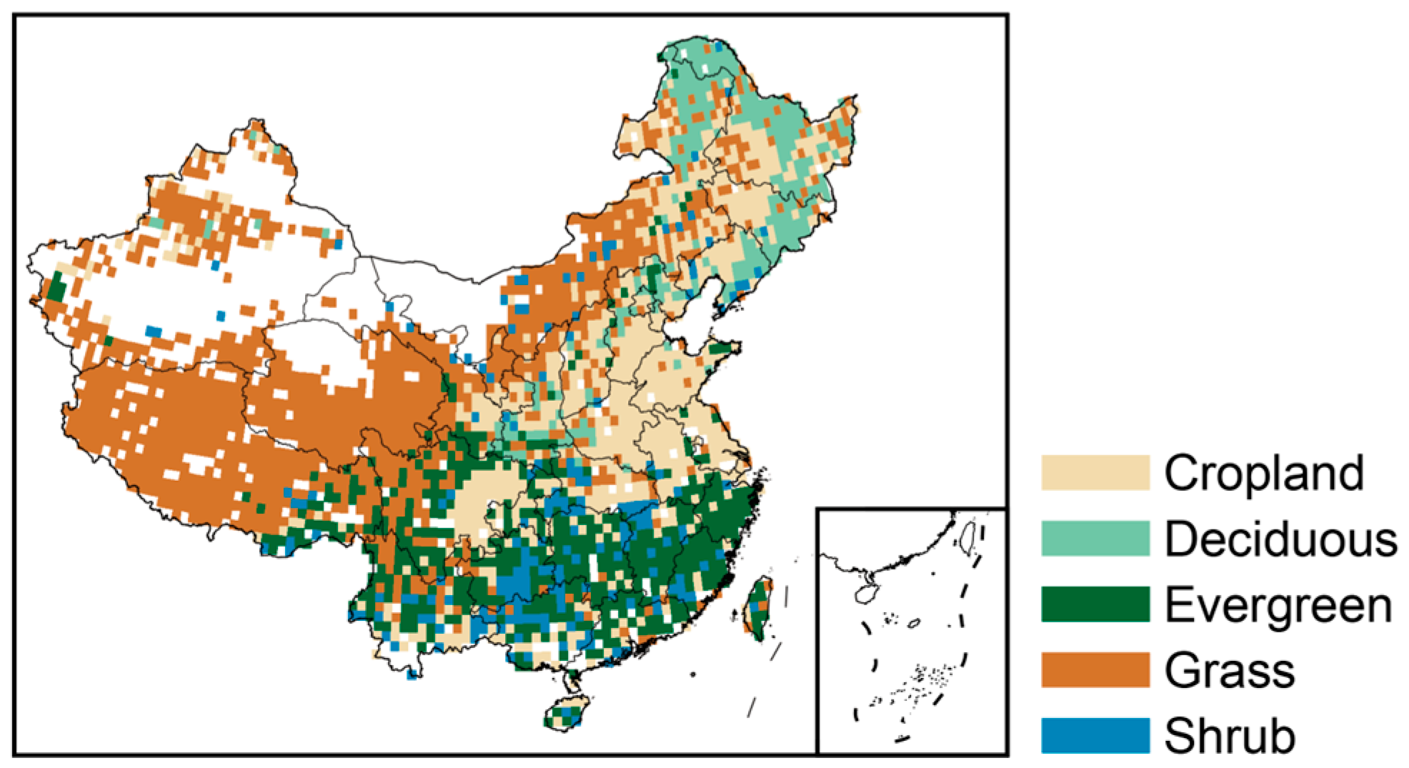
2.1. Study Area

China, extending between 75° E and 135° E in longitude and 18° N to 54° N in latitude, encompasses a vast land area of 9.6 × 10⁶ km2. Marked by diverse climatic zones ranging from arid to humid regions, exhibiting a distinct gradient from its northwest to southeast, China demonstrates a wide range of mean annual temperatures (MAT) and precipitation (MAP) across the country, from 4 °C to 20 °C in MAT and 20 mm to 2000 mm in MAP. This diversity creates a spectrum of environmental conditions that support a variety of ecosystems. Forests, grasslands, shrublands, and croplands in China are distributed across diverse geographical and climatic zones. Deciduous and evergreen forests flourish in the northeastern and southwestern regions, contributing to China’s woodland cover (Figure 1). In the northwest, arid areas are mainly dominated by grass and shrubs, which can adapt to the conditions of limited water availability. Croplands in China are widely distributed across various regions, including the North China Plain, the Northeast China Plain, and the Yangtze River Delta. China has witnessed notable changes in its climate over the last decades. The impacts of climate change are evident in various aspects, including increased temperature, uneven precipitation, and extreme drought events, which have a significant impact on ecosystems and water resources.
In recent decades, China has experienced significant climatic changes, with impacts that include rising temperatures, uneven precipitation patterns, and more frequent extreme drought events [23,24,25,26,27]. These changes have profound effects on both ecosystems and water resources. Given the critical role water plays in vegetation growth, understanding the shifting responses of different ecosystems to water variability is essential, particularly as air pollution and climate stressors interact. Monitoring these changes is key to predicting future ecosystem stability, water resource management, and agricultural productivity in a rapidly evolving environment.

2.2. Methods

2.2.1. Data and Preprocessing

The PKU GIMMS NDVI4g dataset utilized in this study as a proxy for vegetation growth from 1982 to 2022 is derived using a combination of Advanced Very High-Resolution Radiometer (AVHRR, which is a sensor used in the polar orbit platform series by the National Oceanic and Atmospheric Administration of the United States) and Moderate Resolution Imaging Spectroradiometer (MODIS, which is a large-scale space remote sensing instrument developed by NASA) data integrated with a machine learning model. PKU GIMMS NDVI4g incorporates 3.6 million Landsat images using a back propagation neural network to enhance accuracy by gap filling and eliminating the impact of satellite orbit drift and sensor degradation. With a spatial resolution of 1/12° and a temporal resolution of half a month, this dataset can capture fine-scale vegetation dynamics. To match the temporal and spatial resolution of other datasets, we initially aggregated the biweekly data to monthly using the maximum value composition (MVC) [38] method and then resampled it into 0.5° spatial resolution. NDVI was standardized and de-seasonalized by subtracting the multi-year average of the corresponding month and then dividing by the standard deviation, using the formula:
A n o m a l y i , j = ( N D V I i , j N D V I j ¯ σ j )
where A n o m a l y i , j denotes de-seasonalized NDVI anomaly of month j; σ is the standard deviation of NDVI form month j.
The Standardized Precipitation Evapotranspiration Index (SPEI) was used as the water variation index in this study. SPEI provides a robust and multi-scalar measure of drought conditions, accounting for both precipitation and potential evapotranspiration (PET) [39,40]. Unlike simple water deficit calculations, SPEI incorporates PET, which varies based on temperature, radiation, and wind speed, offering more relevance to ecosystem water stress. To capture the immediate dynamics of vegetation responses to water variation, we used multiple scale grided monthly SPEI data (range from 1 to 24), which was extracted from the Global SPEI database, from the years 1982 to 2022.
The land cover data from Global Land Cover 2000 (GLC2000) were utilized in this study (Figure S2), and are a comprehensive global dataset for the year 2000 covering natural vegetation, croplands, urban areas, and water bodies [37]. They combine satellite imagery, ground observations, and ancillary data sources. GLC2000 combines 22 land cover types based on the LCCS (Land Cover Classification System) classification scheme. In this study, we reclassified the original vegetation map by merging several fine-grained categories. Evergreen broadleaf and needleleaf forests were combined into a single “evergreen forests” class and deciduous needleleaf and broadleaf forests were grouped as “deciduous forests.” Similarly, closed and open shrublands, woody savannas, and savannas were combined into the “shrubs” class. Grasslands remained unchanged (“grass”). Finally, the reclassified map was resampled to a 0.5° spatial resolution for consistency with other datasets.
This study employed the widely used Aridity Index (AI) to identify arid and humid zones (Figure 1), which is based on the long-term imbalance between precipitation (P) and potential evapotranspiration (PET) [41,42,43]. If precipitation consistently exceeds evaporation, the area is considered humid; conversely, if evaporation dominates, it is classified as arid. This can be calculated by the following formula:
A I = P / P E T

2.2.2. Analysis of the Relationships between Vegetation and Water Variation

To investigate the relationships between vegetation and water variation, we employ sensitivity and lag analysis. For sensitivity assessment, we perform a Pearson correlation analysis for the growing season (April to October) between NDVI anomaly and SPEI time series. This analysis examined the strength and direction of the linear relationship between anomalies in NDVI and SPEI at each pixel.
For lag assessment, we conducted a lag analysis to identify the time at which the correlation relationship between NDVI and SPEI was strongest [44,45,46]. This involved calculating correlation coefficients with different lags by postponing the NDVI anomaly series relative to 1 to 5 months to SPEI. Lag analysis can be represented by this formula:
L a g = a r g m a x ( c o r r ( S P E I , N D V I n ) )     n [ 1 , 5 ]
where c o r r S P E I , N D V I n denotes the correlation coefficient of SPEI and NDVI at lag n months, n is an integer, and argmax means finding the lag value n with the largest absolute value. The lag effect observed between vegetation and water variability serves as an indicator for assessing the resistance and recovery of ecosystems during droughts. A shorter lag indicates a faster response to water variation, and thus a lower resistance to or higher recovery from droughts [10].
Similar to the lag assessment, we calculated the cumulative timescale of water variation. This is determined by the number of antecedent months at which SPEI showed the maximum correlation with vegetation activity [27]. The cumulative timescale can be expressed as follows:
T c u m = a r g m a x ( c o r r ( S P E I i , N D V I ) )     i [ 1 , 12 ]
where c o r r ( S P E I i , N D V I ) denotes the correlation coefficient of SPEI and NDVI, i is the SPEI scale, which can be represented as cumulative time, and argmax means finding the cumulative time i with the largest absolute value.
To assess the dynamics of the relationship between vegetation and water variations spanning the period from 1982 to 2022, we utilized a 10-year moving window approach. In each window, we calculated sensitivity (correlation coefficients), lag (optimal time delay), and cumulative timescale. For sensitivity, this can be represented by the following formulas:
N D V I n = N D V I n : n + W     n [ 1 , N W + 1 ]
R n = c o r r ( N D V I n , S P E I n )   n [ 1 , N W + 1 ]
R m o v i n g _ w i n d o w = R 1 , R 2 , , R ( N W + 1 )
where N D V I n represent the time series in the nth window, N is the sample size of the time series, and W is moving window size. Rn denotes the sensitivity in the nth window and R m o v i n g _ w i n d o w is the new time series of moving window sensitivities. The methods of lag and cumulative time are similar to sensitivity.

3. Results

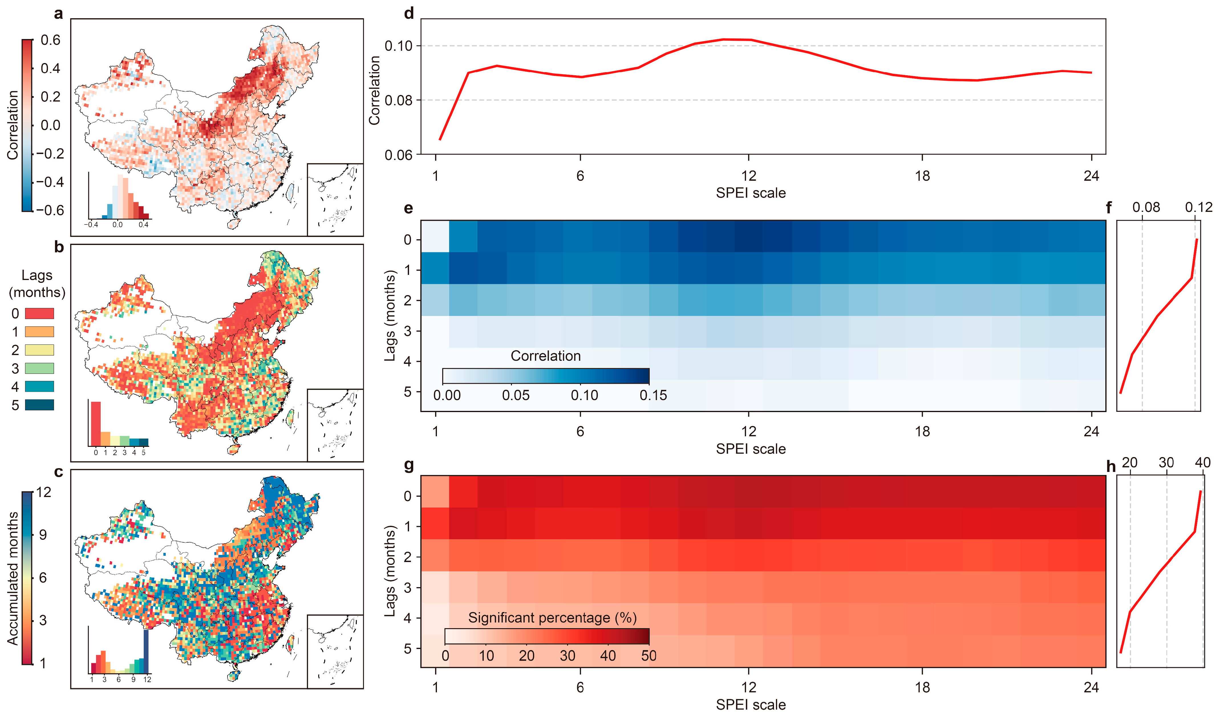
3.1. Sensitivity and Lag Response between Vegetation and Water Variation

We first employ the correlation relationship between mean growing season (May to October) NDVI and multi-scale SPEI (SPEI 1 to 24) to assess the sensitivity of vegetation growth to water variability. Our findings indicate that there is a positive sensitivity between vegetation growth and water variation across 83% of China, and the average correlation coefficient is 0.32 (Figure 2a). Higher positive sensitivity can be found in Inner Mongolia; across this region, the mean correlation coefficient is above 0.4; negative sensitivity is found in the Northeast of China, with an average correlation coefficient of approximately −0.2. We then examined time lags spanning from 0 to 5 months, and for each time lag, we calculated correlation coefficients between NDVI and SPEI 1 to 24 (Figure 2e), the corresponding percentage of significant (p < 0.01) correlations at each time lag is also determined (Figure 2g). By comparing the sensitivity among multiple SPEI scales, we found that longer SPEI scales have higher sensitivity (Figure 2d). We noted that as the lag increases, the sensitivity (percentage of significance) decreases and the correlation coefficients (percentage of significance) range from 0.12 to 0.06 (from 39% to 17%) (Figure 2f,h).
By identifying the time lag associated with the highest positive correlation, we then determined the response lag between vegetation growth and water variation (see Methods). Shorter response lags are widely observed across China, with over 66% of area exhibiting lags of less than 1-month; higher sensitivity usually consistently corresponds to shorter response lags (Figure 2b). The spatial patterns of the optimum cumulative time scale are shown in Figure 2c; regions in Inner Mongolia and Southeast China exhibited shorter cumulative time scales (less than 6 months), suggesting the ecosystem responds primarily to recent water variations. Conversely, northeastern and southwestern China displayed maximum correlations with longer SPEI timescales (greater than 9 months), indicating that vegetation in these areas responds to longer cumulative water variations.
We further explored the sensitivity and response lag as aridity gradient and plant functional types based on multiple SPEI scales. The sensitivity decreases from drier regions to wetter regions, ranging from 0.23 to 0.02 (Figure 3a), which means that regions with lower moisture levels exhibit greater sensitivity. For different plant functional types (Figure 3b), higher sensitivity was found in grass and crops (correlation coefficients are 0.17 and 0.16, respectively); deciduous forests exhibit a weaker connection between vegetation and water supply (correlation coefficient is 0.06). The response lag increases from drier regions to wetter regions, ranging from 1 to 3 months (Figure 3c). For different plant functional types (Figure 3d), deciduous forests exhibited the longest response lag (2.4 months), while grass and crops demonstrated relatively shorter response lags (1.2 and 1.1 months, respectively).

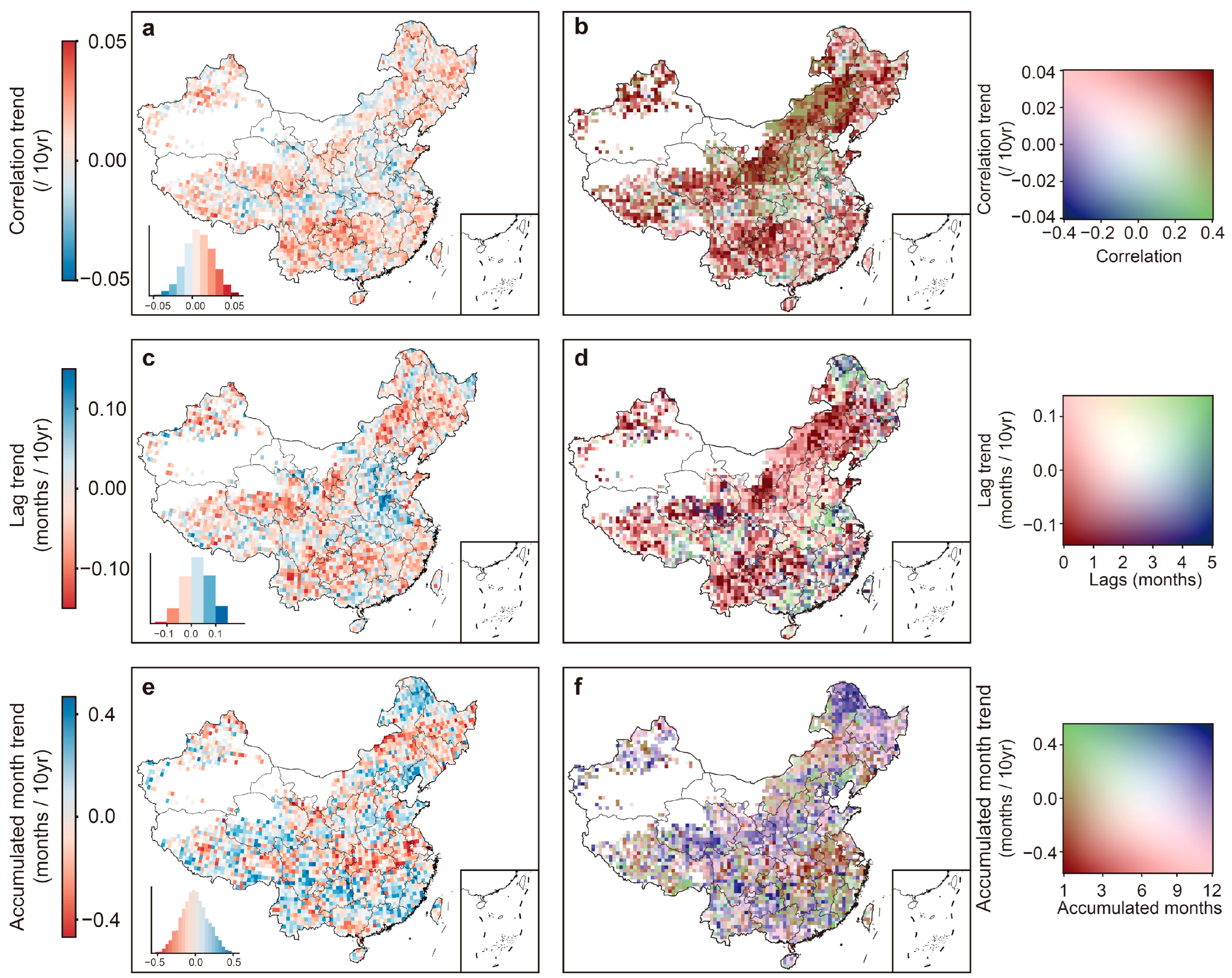
3.2. Increased Sensitivity and Accelerated Response of Vegetation to Water Availability

To identify the temporal evolution of vegetation sensitivity and response lag to water variability, we performed a moving window correlation analysis using a 10-year window size for NDVI vs multi-scale SPEI (see Section 2.2). We found an increasing trend in sensitivity and a simultaneous decline in lag response across all SPEI scales and various plant functional types. The sensitivity to temporal changes displayed a positive slope increase of 0.06 per decade (p < 0.01) (Figure 4a), whereas the temporal evolution of lag response indicated a decrease of 0.18 months per decade (p < 0.01) (Figure 4b). Among various plant functional types, the slope of the temporal change in sensitivity ranged from 0.04 to 0.06 per decade (p < 0.01) (Figure 4a), and the slope of the temporal change in lag response spanned from 0.16 to 0.19 months per decade (p < 0.01) (Figure 4b). Evergreen forests and shrubs exhibited the most pronounced increase in sensitivity, with slope increases of 0.07 and 0.06 (p < 0.01); grass and deciduous forests exhibited the most significant decrease in lag response, with slope decreases of 0.17 and 0.18 months per decade (p < 0.01). For the temporal change in the cumulative water variation effect, we did not find a significant trend from 1982 to 2022, either from the whole region or each plant functional type.
To avoid pre-selecting a specific time lag for analyzing sensitivity trends, we examined a range of lags from 1 to 5 months combined with multiple SPEI timescales (Figure 5a–e). Additionally, we considered the optimal lag for each pixel, defined as the lag with the highest correlation coefficient (Figure 5f). We found that only at a lag of 1 month did we observe a significant increase in sensitivity, with a trend of 0.02 per decade. For longer lags (2–5 months), no significant increase in sensitivity trends was detected. However, using the optimal lag for each pixel, we observed a clear and significant increasing trend in sensitivity, with a trend of 0.01 per decade.
Furthermore, our analysis of spatial trends in sensitivity (Figure 6a) reveals that over 66% of China’s area exhibits an increase in sensitivity to water availability. Notably, southwestern China displays the strongest positive trends, with sensitivity increasing by approximately 0.04 per decade. In contrast, the North China Plain shows a decline in sensitivity, with a trend of 0.03 per decade. Interestingly, vegetation with higher baseline sensitivity is more likely to experience a further increase in sensitivity over time (Figure 6b), where more than 19% of the area with sensitivity exceeding 0.2 exhibits a significant positive trend. When examining the spatial distribution of response lag trends (Figure 6c), we found that over 63% of China exhibits a shortening lag, indicating faster vegetation responses to water changes. Southwestern China again stands out, with a decline in response lag of 0.14 months per decade, signifying a faster response. Conversely, the North China Plain shows an increase in response lag, suggesting a slower response, with a trend of 0.15 months per decade. Vegetation with a shorter response lag (less than 1 month) is more likely to experience a further decrease in lag over time (Figure 6d). Over 21% of these areas exhibit a significant negative trend in lag response. This suggests that vegetation with a faster initial response is becoming even more responsive to water changes. To further validate the robustness of our trend analysis, we examined sensitivity and response lag trends across a range of SPEI timescales (1 to 24 months) (Figure S1). The consistent patterns across these timescales strengthen our confidence in the identified trends and suggest they are not driven by specific choices in the timescale. Analysis of cumulative time scale trends (Figure 6e,f) reveals a contrasting pattern across China: a shortening trend of approximately −0.4 months per decade is evident in the Yangtze River Basin and parts of Northeast China. Conversely, a lengthening trend of around 0.4 months per decade was observed in southern and southwestern regions. Notably, a substantial portion of China (over 48%) exhibited an increasing cumulative time scale with a positive trend.

4. Discussion

4.1. Possible Reasons for Regional Variability in Sensitivity and Lag Response between Vegetation and Water Variation

The sensitivity of vegetation growth to water variability is a key indicator of the impact of drought on ecosystems [4,9,47,48,49]. Our finding confirmed that ecosystems in drier regions have a higher sensitivity to water availability, indicating that they are more vulnerable to droughts, which was consistent with previous studies [4,5,8,50]. Across China, drier environments often experience higher temperatures and increased evaporation rates, which can exacerbate evaporation and intensify water stress, leading to a faster depletion of available moisture and negatively impacting the physiological processes of plants [51,52]. Consequently, vegetation is more sensitive to water availability [53]. Our finding further showed that deciduous and evergreen forests are less sensitive to water variation as they have deeper root systems and high water storage capacity. In contrast, grasses, shrubs, and crops are more sensitive to water availability, as they have shallow root systems and lower water storage capacity [54,55,56]. This is consistent with previous studies that have found that the sensitivity is more pronounced in shallow-rooted vegetation than in deep-rooted vegetation [5,57].
Vegetation in arid regions typically demonstrates a faster response to drought conditions; the reliance on immediate precipitation for water availability makes vegetation less resistant to water stress. Conversely, when precipitation occurs following a drought, plants in these regions exhibit a swift response, efficiently utilizing the available moisture. This process results in a shorter time lag, reflecting the rapid recovery and increased vegetation activity following water supply [58].
Different SPEI scales (e.g., 1-month, 3-month, 6-month) reflect water conditions over varying periods, influencing vegetation responses [2,44,59,60]. We observed similar lags across multiple SPEI scales (Figure 2e,f), suggesting a consistent response pattern of vegetation to changes in water availability. This consistency could be due to the intrinsic vegetation response time, meaning vegetation may have inherent physiological response times to changes in water availability, leading to a consistent lag regardless of the timescale of water variation.

4.2. Possible Reasons for Intensified Vegetation Sensitivity and Shortened Response Lag to Water Variation

Vegetation sensitivity to water variability has intensified over the past 40 years, coupled with a corresponding reduction in response lag (Figure 4a,b). This indicates a heightened promptness in the vegetation growth response to water variability compared to previous decades. Global warming has contributed to a widespread “greening” trend in ecosystems across the Northern Hemisphere [61,62]. However, this apparent increase in greenness is accompanied by elevated transpiration rates, leading to a higher demand for water from the soil [24,63]. Consequently, intensified transpiration exacerbates vegetation stress, resulting in an increased sensitivity to drought and a reduction in lag time. Besides global warming, human activity such as greening reforestation programs, including the Three-North Shelterbelt Development Program and Grain for Green Program, may deplete soil water or groundwater and thus intensify water stress [64], which could intensify plant sensitivity over time. Over time, there has been a decrease in sensitivity between crops and SPEI among all plant functional types. This decoupling may be attributed to the increased extraction of groundwater for irrigation [65,66]. Nevertheless, this heightened extraction has led to irreversible declines in groundwater storage, subsequently diminishing groundwater discharge to streams and rivers. Consequently, ecosystems reliant on groundwater are poised to endure more severe impacts during droughts [67]. Furthermore, the increased severity and frequency of drought events in arid regions, compounded by elevated temperatures that contribute to higher water evaporation rates, place vegetation under greater pressure from water scarcity, which further amplifies its sensitivity to drought [68].
Land use change may also significantly affect vegetation sensitivity and lag response over time by altering water availability, soil properties, and ecosystem dynamics [69,70]. Urbanization, deforestation, and agricultural expansion often reduce vegetation cover [71], disrupt hydrological cycles, and lower soil moisture retention, making ecosystems more sensitive to water variability. For example, deforestation decreases the water-holding capacity of soils [72], leading to quicker depletion of moisture during droughts and reducing the lag between precipitation and vegetation response. Similarly, the conversion of natural landscapes to agricultural land increases water demand for irrigation, often exacerbating water stress and further reducing response times. Over time, these changes intensify the sensitivity of ecosystems to climate variability and water scarcity, making sustainable land management essential to prevent degradation.
Although more than 66% of regions have shown increasing sensitivity and decreasing lag response over time, it is interesting to note that Inner Mongolia, an arid region, exhibits decreasing sensitivity and increasing response lag. Such decoupling could be partially attributed to increased groundwater levels over the past decade, which have helped buffer plant water stress in these regions [73]. Moreover, a decreasing drought sensitivity over time in Inner Mongolia suggests that plants are adapting to droughts and adjusting their water use strategies by tapping water from deeper soil water, rocks, and groundwater [74]. In contrast, southern China, classified as a humid region, is also becoming more sensitive, likely due to decreased groundwater and soil moisture [75], which intensifies plants’ vulnerability to droughts.
Although there seems to be no trend in the cumulative time scale from 1982 to 2022 (Figure 4c), the spatial pattern of cumulative drought effect trends varies across different regions and aligns with the spatial patterns of lag and sensitivity trends (Figure 6a,c,e), especially in northeastern China and the Yangtze River Basin. The shortened lag and shortened cumulative timescale are interconnected. When vegetation responds more quickly to water stress (shortened lag), it indicates that plants are experiencing immediate water deficits rather than relying on stored soil moisture or longer-term water availability. This rapid response reduces the period over which drought effects accumulate, leading to a shortened cumulative timescale.

4.3. Implications for Future Ecosystem Management and Water Resource Planning

The increasing sensitivity of vegetation to water variability and the shortening lag response highlight crucial challenges for future ecosystem management and water resource planning. As ecosystems become more sensitive to drought, particularly in arid and semi-arid regions, land managers will need to prioritize strategies that enhance ecosystem resilience to water stress using drought-resistant species, improving soil moisture retention, and regulating groundwater use to prevent over-extraction. As vegetation responds more rapidly to water deficits, timely intervention in water resource management is important, especially in regions facing frequent or prolonged droughts. Adaptive water management frameworks that account for these changing dynamics will be crucial for maintaining ecosystem activity and preventing irreversible degradation.

4.4. Limitations and Future Research Directions

There are several limitations in this research that need to be acknowledged. First, while the GIMMS NDVI4g data provide a long-term record of vegetation dynamics, resampling their spatial resolution to 0.5 degrees to match the SPEI data may lead to a loss of finer spatial details, particularly in regions with heterogeneous landscapes. Second, the use of SPEI, although effective in capturing water stress, might not account for other relevant factors influencing vegetation responses, such as soil properties or local water management practices, which could affect the accuracy of sensitivity and lag assessments. Additionally, while the aridity index and GLC2000 data provide a useful framework for categorizing climate zones and plant functional types, they may not fully reflect dynamic land cover changes or more recent developments in vegetation classification since these datasets are based on earlier periods. Lastly, the reliance on correlation and lag analysis may overlook complex interactions between climate variables and vegetation responses, suggesting the need for more comprehensive models that integrate multiple environmental drivers. These limitations highlight areas for further refinement and the incorporation of additional datasets to provide a more holistic understanding of vegetation–water interactions.
While our findings highlight the increasing sensitivity of vegetation to water variability, the underlying mechanisms driving this trend remain unclear. The correlation between NDVI and SPEI provides valuable insights but does not fully explain the physiological and ecological processes involved. Understanding these mechanisms is critical for predicting how ecosystems will respond to ongoing climate change. Therefore, further research is needed to integrate data on plant physiology, soil moisture dynamics, and atmospheric conditions to establish clearer causal links. Such studies would improve our predictive understanding of ecosystem responses and help refine earth system models, which are essential for accurate and effective ecosystem management. In addition, this mechanistic understanding would enable the development of targeted mitigation strategies aimed at reducing vegetation vulnerability to future climate stressors.

5. Conclusions

In conclusion, our study sheds light on the critical importance of understanding how plants adapt to evolving water availability, especially in the context of predicting ecosystem vulnerability to drought and managing resources amidst climate change challenges. By leveraging the latest GIMMS NDVI4g and SPEI, we explored the spatial–temporal dynamics of sensitivity and lag in vegetation growth in response to water variability across China from 1982 to 2022. Our findings reveal that a substantial portion of China’s vegetation, exceeding 66%, exhibits heightened sensitivity to water availability, with 63% displaying a shorter response lag. This sensitivity varies across aridity gradients and among different plant functional types. Moreover, over the past decades, most of China’s vegetation has demonstrated increased sensitivity to water variability, accompanied by a shorter response lag. These outcomes significantly contribute to our understanding of vegetation dynamics in the face of changing water conditions, pointing towards an increased susceptibility of vegetation to drought in a future warming world. The insights gained from this study underscore the urgency of adopting proactive measures to address the potential impacts of shifting water availability on ecosystems, emphasizing the importance of sustainable resource management practices in the context of a changing climate.

Supplementary Materials

The following supporting information can be downloaded at: https://www.mdpi.com/article/10.3390/w16182677/s1, Figure S1: Violin plots of the distribution of trends in (a) sensitivity and (b) response lag for each SPEI timescale (1 to 24 months). The caps represent the minimum and maximum values, the whiskers represent the 25th, 50th, and 75th percentiles; Figure S2: Spatial distribution of aridity index.

Author Contributions

H.T. designed the experiments, analyzed the data, and wrote the original draft. Y.L. wrote and conceived the idea. J.F. Validation. J.Y. Edited, reviewed, and supervised. All authors have read and agreed to the published version of the manuscript.

Funding

This study was partially supported by the Anhui Province University Research Project (No. 2024AH051857), the Anhui University Excellent Research and Innovation Project (No. 2022AH010094).

Data Availability Statement

The data presented in this study are available on request from the corresponding author.

Conflicts of Interest

The authors declare no competing interests.

References

  1. Gazol, A.; Camarero, J.J.; Anderegg, W.R.L.; Vicente-Serrano, S.M. Biogeography. Impacts of droughts on the growth resilience of Northern Hemisphere forests. Glob. Ecol. Biogeogr. 2017, 26, 166–176. [Google Scholar] [CrossRef]
  2. Vicente-Serrano, S.M.; Gouveia, C.; Camarero, J.J.; Beguería, S.; Trigo, R.; Lopez-Moreno, J.I.; Azorin-Molina, C.; Pasho, E.; Lorenzo-Lacruz, J.; Revuelto, J.; et al. Response of vegetation to drought time-scales across global land biomes. Proc. Natl. Acad. Sci. USA 2012, 110, 52–57. [Google Scholar] [CrossRef]
  3. Zhao, X.; Wei, H.; Liang, S.; Zhou, T.; He, B.; Tang, B.; Wu, D. Responses of Natural Vegetation to Different Stages of Extreme Drought during 2009–2010 in Southwestern China. Remote Sens. 2015, 7, 14039–14054. [Google Scholar] [CrossRef]
  4. Jiao, W.; Wang, L.; Smith, W.K.; Chang, Q.; Wang, H.; D’odorico, P. Observed increasing water constraint on vegetation growth over the last three decades. Nat. Commun. 2021, 12, 3777–3786. [Google Scholar] [CrossRef] [PubMed]
  5. Xu, H.-J.; Wang, X.-P.; Zhao, C.-Y.; Yang, X.-M. Diverse responses of vegetation growth to meteorological drought across climate zones and land biomes in northern China from 1981 to 2014. Agric. For. Meteorol. 2018, 262, 1–13. [Google Scholar] [CrossRef]
  6. Gu, X.; Guo, E.; Yin, S.; Wang, Y.; Mandula, N.; Wan, Z.; Yun, X.; Li, H.; Bao, Y. Differentiating cumulative and lagged effects of drought on vegetation growth over the Mongolian Plateau. Ecosphere 2022, 13, e4289–e4309. [Google Scholar] [CrossRef]
  7. Hua, L.; Wang, H.; Sui, H.; Wardlow, B.; Hayes, M.J.; Wang, J. Mapping the Spatial-Temporal Dynamics of Vegetation Response Lag to Drought in a Semi-Arid Region. Remote Sens. 2019, 11, 1873. [Google Scholar] [CrossRef]
  8. Zhang, W.; Li, Y.; Wu, X.; Chen, Y.; Chen, A.; Schwalm, C.R.; Kimball, J.S. Divergent response of vegetation growth to soil water availability in dry and wet periods over Central Asia: Biogeosciences. J. Geophys. Res. Biogeosci. 2021, 126, e2020JG005912. [Google Scholar] [CrossRef]
  9. Jiao, W.; Chang, Q.; Wang, L. The sensitivity of satellite solar-induced chlorophyll fluorescence (SIF) to meteorological drought. Earth’s Future 2019, 7, 558–573. [Google Scholar] [CrossRef]
  10. Li, Y.; Zhang, W.; Schwalm, C.R.; Gentine, P.; Smith, W.K.; Ciais, P.; Kimball, J.S.; Gazol, A.; Kannenberg, S.A.; Chen, A.; et al. Widespread spring phenology effects on drought recovery of Northern Hemisphere ecosystems. Nat. Clim. Chang. 2023, 13, 182–188. [Google Scholar] [CrossRef]
  11. Miller, D.L.; Wolf, S.; Fisher, J.B.; Zaitchik, B.F.; Xiao, J.; Keenan, T.F. Increased photosynthesis during spring drought in energy-limited ecosystems. Nat. Commun. 2023, 14, 7828. [Google Scholar] [CrossRef] [PubMed]
  12. Sun, Y.; Fu, R.; Dickinson, R.; Joiner, J.; Frankenberg, C.; Gu, L.; Xia, Y.; Fernando, N. Satellite solar-induced chlorophyll fluorescence reveals drought onset mechanisms: Insights from two contrasting extreme events. J. Geophys. Res. Biogeosci. 2015, 120, 2427–2440. [Google Scholar] [CrossRef]
  13. Zhang, L.; Qiao, N.; Huang, C.; Wang, S. Monitoring Drought Effects on Vegetation Productivity Using Satellite Solar-Induced Chlorophyll Fluorescence. Remote Sens. 2019, 11, 378. [Google Scholar] [CrossRef]
  14. Afshar, M.H.; Al-Yaari, A.; Yilmaz, M.T. Comparative Evaluation of Microwave L-Band VOD and Optical NDVI for Agriculture Drought Detection over Central Europe. Remote Sens. 2021, 13, 1251. [Google Scholar] [CrossRef]
  15. Lawal, S. On the suitability of using Vegetation Indices to monitor the response of Africa’s terrestrial ecoregions to drought. Sci. Total Environ. 2021, 792, 148282. [Google Scholar] [CrossRef]
  16. Wang, Z.; Wang, H.; Wang, T.; Wang, L.; Liu, X.; Zheng, K.; Huang, X. Large discrepancies of global greening: Indication of multi-source remote sensing data. Glob. Ecol. Conserv. 2022, 34, e02016. [Google Scholar] [CrossRef]
  17. Chen, C.; Park, T.; Wang, X.; Piao, S.; Xu, B.; Chaturvedi, R.K.; Fuchs, R.; Brovkin, V.; Ciais, P.; Fensholt, R.; et al. China and India lead in greening of the world through land-use management. Nat. Sustain. 2019, 2, 122–129. [Google Scholar] [CrossRef]
  18. Li, M.; Cao, S.; Zhu, Z.; Wang, Z.; Myneni, R.B.; Piao, S. Spatiotemporally consistent global dataset of the GIMMS Normalized Difference Vegetation Index (PKU GIMMS NDVI) from 1982 to 2022. Earth Syst. Sci. Data 2023, 15, 4181–4203. [Google Scholar] [CrossRef]
  19. Piao, S.; Huang, M.; Liu, Z.; Wang, X.; Ciais, P.; Canadell, J.G.; Wang, K.; Bastos, A.; Friedlingstein, P.; Houghton, R.A.; et al. Lower land-use emissions responsible for increased net land carbon sink during the slow warming period. Nat. Geoence 2018, 11, 739–745. [Google Scholar] [CrossRef]
  20. Yang, S.; Sheng, D.; Adamowski, J.; Gong, Y.; Zhang, J.; Cao, J. Effect of Land Use Change on Soil Carbon Storage over the Last 40 Years in the Shi Yang River Basin, China. Land 2018, 7, 11. [Google Scholar] [CrossRef]
  21. Jiang, W.; Wang, L.; Feng, L.; Zhang, M.; Yao, R. Drought characteristics and its impact on changes in surface vegetation from 1981 to 2015 in the Yangtze River Basin, China. Int. J. Climatol. 2020, 40, 3380–3397. [Google Scholar] [CrossRef]
  22. Xu, T.; Wu, X.; Tian, Y.; Li, Y.; Zhang, W.; Zhang, C. Soil Property Plays a Vital Role in Vegetation Drought Recovery in Karst Region of Southwest China. J. Geophys. Res. (Biogeosci.) 2021, 126, 126–140. [Google Scholar] [CrossRef]
  23. Seneviratne, S.I.; Zhang, X.; Adnan, M.; Badi, W.; Dereczynski, C.; Luca, A.D.; Ghosh, S.; Iskandar, I.; Kossin, J.; Lewis, S.; et al. Weather and Climate Extreme Events in a Changing Climate. In Climate Change 2021; Cambridge University Press: Cambridge, UK, 2023; pp. 1513–1766. [Google Scholar] [CrossRef]
  24. Dai, A.; Zhao, T.; Chen, J. Climate Change and Drought: A Precipitation and Evaporation Perspective. Curr. Clim. Chang. Rep. 2018, 4, 301–312. [Google Scholar] [CrossRef]
  25. Park, C.K.; Byun, H.R.; Deo, R.; Lee, B.R. Drought prediction till 2100 under RCP 8.5 climate change scenarios for Korea. J. Hydrol. 2015, 526, 221–230. [Google Scholar] [CrossRef]
  26. Trenberth, K.E.; Dai, A.; Van Der Schrier, G.; Jones, P.D.; Barichivich, J.; Briffa, K.R.; Sheffield, J. Global warming and changes in drought. Nat. Clim. Chang. 2014, 4, 17–22. [Google Scholar] [CrossRef]
  27. Ding, Y.; Xu, J.; Wang, X.; Peng, X.; Cai, H. Spatial and temporal effects of drought on Chinese vegetation under different coverage levels. Sci. Total Environ. 2020, 716, 137166. [Google Scholar] [CrossRef]
  28. Li, J.; Mahalov, A.; Hyde, P. Simulating the effects of chronic ozone exposure on hydrometeorology and crop productivity using a fully coupled crop, meteorology and air quality modeling system. Agric. For. Meteorol. 2018, 260, 287–299. [Google Scholar] [CrossRef]
  29. Yue, X.; Unger, N.; Harper, K.; Xia, X.; Liao, H.; Zhu, T.; Xiao, J.; Feng, Z.; Li, J. Ozone and haze pollution weakens net primary productivity in China. Atmos. Chem. Phys. 2017, 17, 6073–6089. [Google Scholar] [CrossRef]
  30. Zhu, J.; Tai, A.P.K.; Hung Lam Yim, S. Effects of ozone–vegetation interactions on meteorology and air quality in China using a two-way coupled land–atmosphere model. Atmos. Chem. Phys. 2022, 22, 765–782. [Google Scholar] [CrossRef]
  31. Ossohou, M.; Galy-Lacaux, C.; Yoboué, V.; Hickman, J.; Gardrat, E.; Adon, M.; Darras, S.; Laouali, D.; Akpo, A.; Ouafo, M.; et al. Trends and seasonal variability of atmospheric NO2 and HNO3 concentrations across three major African biomes inferred from long-term series of ground-based and satellite measurements. Atmos. Environ. 2019, 207, 148–166. [Google Scholar] [CrossRef]
  32. Adon, M.; Galy-Lacaux, C.; Delon, C.; Yoboue, V.; Solmon, F.; Tchuente, A.T.K. Dry deposition of nitrogen compounds (NO2, HNO3, NH3), sulfur dioxide and ozone in west and central African ecosystems using the inferential method. Atmos. Chem. Phys. 2013, 13, 11351–11374. [Google Scholar] [CrossRef]
  33. Rai, P.K. Impacts of particulate matter pollution on plants: Implications for environmental biomonitoring. Ecotoxicol. Environ. Saf. 2016, 129, 120–136. [Google Scholar] [CrossRef] [PubMed]
  34. Mandal, M.; Das, S.; Roy, A.; Rakwal, R.; Jones, O.A.; Popek, R.; Agrawal, G.K.; Sarkar, A. Interactive relations between plants, the phyllosphere microbial community, and particulate matter pollution. Sci. Total Environ. 2023, 890, 164352. [Google Scholar] [CrossRef] [PubMed]
  35. Tao, W.; Song, M.; Weng, S.; Chen, X.; Cui, L. Assessing the impact of environmental regulation on ecological risk induced by PM2.5 pollution: Evidence from China. J. Clean. Prod. 2024, 451, 142029. [Google Scholar] [CrossRef]
  36. Harris, I.; Osborn, T.J.; Jones, P.; Lister, D. Version 4 of the CRU TS monthly high-resolution gridded multivariate climate dataset. Sci. Data 2020, 7, 109–125. [Google Scholar] [CrossRef]
  37. Bartholome, E.; Belward, A.S. GLC2000: A new approach to global land cover mapping from Earth observation data. Int. J. Remote Sens. 2005, 26, 1959–1977. [Google Scholar] [CrossRef]
  38. Holben, B.N. Characteristics of maximum-value composite images from temporal AVHRR data. Int. J. Remote Sens. 1986, 7, 1417–1434. [Google Scholar] [CrossRef]
  39. Beguería, S.; Vicente-Serrano, S.M.; Reig, F.; Latorre, B. Standardized precipitation evapotranspiration index (SPEI) revisited: Parameter fitting, evapotranspiration models, tools, datasets and drought monitoring. Int. J. Climatol. 2014, 34, 3001–3023. [Google Scholar] [CrossRef]
  40. Vicente-Serrano, S.M.; Beguería, S.; López-Moreno, J.I. A Multiscalar Drought Index Sensitive to Global Warming: The Standardized Precipitation Evapotranspiration Index. J. Clim. 2010, 23, 1696–1718. [Google Scholar] [CrossRef]
  41. Huang, J.; Yu, H.; Guan, X.; Wang, G.; Guo, R. Accelerated dryland expansion under climate change. Nat. Clim. Chang. 2015, 6, 166–171. [Google Scholar] [CrossRef]
  42. Lin, L.; Gettelman, A.; Fu, Q.; Xu, Y. Simulated differences in 21st century aridity due to different scenarios of greenhouse gases and aerosols. Clim. Chang. 2016, 146, 407–422. [Google Scholar] [CrossRef]
  43. Greve, P.; Roderick, M.L.; Ukkola, A.M.; Wada, Y. The aridity Index under global warming. Environ. Res. Lett. 2019, 14, 124006. [Google Scholar] [CrossRef]
  44. Wei, X.; He, W.; Zhou, Y.; Ju, W.; Xiao, J.; Li, X.; Liu, Y.; Xu, S.; Bi, W.; Zhang, X.; et al. Global assessment of lagged and cumulative effects of drought on grassland gross primary production. Ecol. Indic. 2022, 136, 108646. [Google Scholar] [CrossRef]
  45. Wen, Y.; Liu, X.; Pei, F.; Li, X.; Du, G.; Meteorology, F. Non-uniform time-lag effects of terrestrial vegetation responses to asymmetric warming. Agric. For. Meteorol. 2018, 252, 130–143. [Google Scholar] [CrossRef]
  46. Wu, D.; Zhao, X.; Liang, S.; Zhou, T.; Huang, K.; Tang, B.; Zhao, W.Q. Time-lag effects of global vegetation responses to climate change. Glob. Chang. Biol. 2015, 21, 3520–3531. [Google Scholar] [CrossRef]
  47. Zhao, A.; Yu, Q.; Feng, L.; Zhang, A.; Pei, T. Evaluating the cumulative and time-lag effects of drought on grassland vegetation: A case study in the Chinese Loess Plateau. J. Environ. Manag. 2020, 261, 110214. [Google Scholar] [CrossRef]
  48. Wu, X.; Liu, H.; Li, X.; Piao, S.; Ciais, P.; Guo, W.; Yin, Y.; Poulter, B.; Peng, C.; Viovy, N.; et al. Higher Temperature Variability Reduces Temperature Sensitivity of Vegetation Growth in Northern Hemisphere. Geophys. Res. Lett. 2017, 44, 6173–6181. [Google Scholar] [CrossRef]
  49. D’Orangeville, L.; Maxwell, J.; Kneeshaw, D.; Pederson, N.; Duchesne, L.; Logan, T.; Houle, D.; Arseneault, D.; Beier, C.M.; Bishop, D.A.; et al. Drought timing and local climate determine the sensitivity of eastern temperate forests to drought. Glob. Chang. Biol. 2018, 24, 2339–2351. [Google Scholar] [CrossRef]
  50. Knapp, A.K.; Carroll, C.J.W.; Denton, E.M.; La Pierre, K.J.; Collins, S.L.; Smith, M.D. Differential sensitivity to regional-scale drought in six central US grasslands. Oecologia 2015, 177, 949–957. [Google Scholar] [CrossRef]
  51. Miralles, D.G.; Pierre, G.; Seneviratne, S.I.; Teuling, A.J. Land–atmospheric feedbacks during droughts and heatwaves: State of the science and current challenges. Ann. N. Y. Acad. Sci. 2018, 1436, 19–35. [Google Scholar] [CrossRef]
  52. Zhou, S.; Williams, A.P.; Berg, A.M.; Cook, B.I.; Gentine, P. Land–atmosphere feedbacks exacerbate concurrent soil drought and atmospheric aridity. Proc. Natl. Acad. Sci. USA 2019, 116, 18848–18853. [Google Scholar] [CrossRef] [PubMed]
  53. Domeisen, D.I.V.; Eltahir, E.A.B.; Fischer, E.M.; Knutti, R.; Perkins-Kirkpatrick, S.E.; Schär, C.; Seneviratne, S.I.; Weisheimer, A.; Wernli, H. Prediction and projection of heatwaves. Nat. Rev. Earth Environ. 2022, 4, 36–50. [Google Scholar] [CrossRef]
  54. Sun, S.; Sun, G.; Caldwell, P.; McNulty, S.; Cohen, E.; Xiao, J.; Zhang, Y. Drought impacts on ecosystem functions of the U.S. National Forests and Grasslands: Part II assessment results and management implications. For. Ecol. Manag. 2015, 353, 269–279. [Google Scholar] [CrossRef]
  55. Wolf, S.; Eugster, W.; Ammann, C.; Häni, M.; Zielis, S.; Hiller, R.; Stieger, J.; Imer, D.; Merbold, L.; Buchmann, N. Contrasting response of grassland versus forest carbon and water fluxes to spring drought in Switzerland. Environ. Res. Lett. 2013, 8, 1345–1346. [Google Scholar] [CrossRef]
  56. Wu, X.; Liu, H.; Li, X.; Ciais, P.; Babst, F.; Guo, W.; Zhang, C.; Magliulo, V.; Pavelka, M.; Liu, S.; et al. Differentiating drought legacy effects on vegetation growth over the temperate Northern Hemisphere. Glob. Chang. Biol. 2017, 24, 504–516. [Google Scholar] [CrossRef] [PubMed]
  57. Lei, T.; Wu, J.; Li, X.; Geng, G.; Shao, C.; Zhou, H.; Wang, Q.; Liu, L. A new framework for evaluating the impacts of drought on net primary productivity of grassland. Sci. Total Environ. 2015, 536, 161–172. [Google Scholar] [CrossRef]
  58. Wei, W.; Liu, T.; Zhou, L.; Wang, J.; Yan, P.; Xie, B.; Zhou, J. Drought-Related Spatiotemporal Cumulative and Time-Lag Effects on Terrestrial Vegetation across China. Remote Sens. 2023, 15, 4362. [Google Scholar] [CrossRef]
  59. Xu, S.; Wang, Y.; Liu, Y.; Li, J.; Qian, K.; Yang, X.; Ma, X. Evaluating the cumulative and time-lag effects of vegetation response to drought in Central Asia under changing environments. J. Hydrol. 2023, 627, 130455. [Google Scholar] [CrossRef]
  60. Zhan, C.; Liang, C.; Zhao, L.; Jiang, S.; Niu, K.; Zhang, Y. Drought-related cumulative and time-lag effects on vegetation dynamics across the Yellow River Basin, China. Ecol. Indic. 2022, 143, 109409. [Google Scholar] [CrossRef]
  61. Lian, X.; Piao, S.; Chen, A.; Wang, K.; Myneni, R.B. Seasonal biological carryover dominates northern vegetation growth. Nat. Commun. 2021, 12, 983–992. [Google Scholar] [CrossRef]
  62. Piao, S.; Wang, X.; Park, T. Characteristics, drivers and feedbacks of global greening. Nat. Rev. Earth Environ. 2020, 1, 14–27. [Google Scholar] [CrossRef]
  63. Ma, N.; Zhang, Y.; Guo, Y.; Gao, H.; Zhang, H.; Wang, Y.F. Environmental and biophysical controls on the evapotranspiration over the highest alpine steppe. J. Hydrol. 2015, 529, 980–992. [Google Scholar] [CrossRef]
  64. Li, C.; Fu, B.; Wang, S.; Stringer, L.C.; Wang, Y.; Li, Z.; Liu, Y.; Zhou, W. Drivers and impacts of changes in China’s drylands. Nat. Rev. Earth Environ. 2021, 2, 858–873. [Google Scholar] [CrossRef]
  65. Yang, F.; Jia, C.; Yang, H.; Yang, X. Development, hotspots and trend directions of groundwater salinization research in both coastal and inland areas: A bibliometric and visualization analysis from 1970 to 2021. Environ. Sci. Pollut. Res. 2022, 29, 67704–67727. [Google Scholar] [CrossRef] [PubMed]
  66. Aeschbach-Hertig, W.; Gleeson, T. Regional strategies for the accelerating global problem of groundwater depletion. Nat. Geosci. 2012, 5, 853–861. [Google Scholar] [CrossRef]
  67. Kløve, B.; Ala-Aho, P.; Bertrand, G.; Gurdak, J.J.; Kupfersberger, H.; Kværner, J.; Muotka, T.; Mykrä, H.; Preda, E.; Rossi, P.; et al. Climate change impacts on groundwater and dependent ecosystems. J. Hydrol. 2014, 518, 250–266. [Google Scholar] [CrossRef]
  68. Zhao, M.; Geruo, A.; Liu, Y.; Konings, A.G. Evapotranspiration frequently increases during droughts. Nat. Clim. Chang. 2022, 12, 1024–1030. [Google Scholar] [CrossRef]
  69. Zhang, Y.; Gentine, P.; Luo, X.; Lian, X.; Liu, Y.; Zhou, S.; Michalak, A.M.; Sun, W.; Fisher, J.B.; Piao, S.; et al. Increasing sensitivity of dryland vegetation greenness to precipitation due to rising atmospheric CO2. Nat. Commun. 2022, 13, 4875. [Google Scholar] [CrossRef]
  70. Wang, X.; Zhao, F.; Wu, Y. Increased sensitivity of vegetation to soil moisture and its key mechanisms in the Loess Plateau, China. Ecohydrology 2024, 17, e2602. [Google Scholar] [CrossRef]
  71. Yang, K.; Sun, W.; Luo, Y.; Zhao, L. Impact of urban expansion on vegetation: The case of China (2000–2018). J. Environ. Manag. 2021, 291, 112598. [Google Scholar] [CrossRef]
  72. Mompremier, R.; Her, Y.; Hoogenboom, G.; Song, J. Effects of deforestation and afforestation on water availability for dry bean production in Haiti. Agric. Ecosyst. Environ. Dev. Sustain. 2022, 325, 107721. [Google Scholar] [CrossRef]
  73. Chiloane, C.; Shoko, C. Impacts of Groundwater and Climate Variability on Terrestrial Groundwater Dependent Ecosystems: A Review of Geospatial Assessment Approaches and Challenges and Possible Future Research Directions. Geocarto Int. 2021, 37, 6755–6779. [Google Scholar] [CrossRef]
  74. Miguez-Macho, G.; Fan, Y. Spatiotemporal origin of soil water taken up by vegetation. Nature 2021, 598, 624–628. [Google Scholar] [CrossRef]
  75. Lin, X.; Li, W.; Bai, X.; Han, L.; Ming, D. Spatial variation in groundwater depletion across China under multiple stresses. Front. Environ. Sci. 2022, 10, 1067766. [Google Scholar] [CrossRef]
Figure 1. Plant functional types derived from Global Land Cover 2000 (GLC2000).
Water 16 02677 g001
Figure 2. Spatial Patterns and Average Values of Sensitivity, Response Lag, and Optimal SPEI Scale Across China. Spatial distribution of (a) sensitivity, (b) response lag (in months), and (c) cumulative time scale across China. The histogram of each spatial distribution is embedded in the lower left corner. (e) Shows the average sensitivity for all pixels across different lags (0 to 5 months) based on SPEI 1 to 24, while (g) highlights the percentage with statistically significant sensitivity (p < 0.01). (d) Shows average sensitivity across different SPEI scales. (f,h) Depict the average sensitivity and percentage of statistically significant values for each lag.
Water 16 02677 g002
Figure 3. Sensitivity and Response Lags Across Aridity Gradient and Plant Functional Types. (a,c) Show sensitivity and lags along the aridity index gradient based on SPEI 1 to 24; the top of each panel shows the average sensitivity and response lag within each aridity index bin. The shaded area represents the probability distribution of the aridity index. (b,d) Show sensitivity and response lags for different plant functional types; error bars indicate standard deviations.
Water 16 02677 g003
Figure 4. Temporal Trends in Sensitivity and Response Lag (1982–2022). Trends in (a) sensitivity (b) response lag (in months) and (c) cumulative time scale across China from 1982 to 2022, based on a 10-year moving window analysis. Gray lines represent individual SPEI timescales (1 to 24 months). Colored dashed lines represent the average values for different plant functional types. The thick red line shows the overall average sensitivity or response lag for all SPEI scales and plant functional types. The black dashed line represents the linear fit line for the overall average values.
Water 16 02677 g004
Figure 5. Sensitivity Trends Across Different Response Lags (1982–2022). (ae) Show trends in sensitivity across China from 1982 to 2022, based on a 10-year moving window analysis, for different response lags (1 to 5 months); each panel shows the sensitivity for a specific lag. (f) Shows trends in sensitivity based on the optimal lag (the lag with the maximum average sensitivity). Gray lines represent individual SPEI timescales (1 to 24 months). The thick red line shows the overall average sensitivity or response lag for all SPEI scales and plant functional types. The black dashed line represents the linear fit line for the overall average values.
Water 16 02677 g005
Figure 6. Spatial and Temporal Trends in Sensitivity and Response Lag (1982–2022). Spatial distribution of trends in (a) sensitivity, (c) response lag (in months), and (e) cumulative time scale across China from 1982 to 2022. (Sensitivity and lag are the average of SPEI 1 to 24 months.) Bivariate color maps display the relationship between long-term average values (1982–2022) and temporal trends for (b) sensitivity, (d) response lag, and (f) cumulative time scale. The color legend’s horizontal axis represents the long-term average sensitivity, lag, or cumulative time scale. The vertical axis reflects the trends in sensitivity, lag, or cumulative time scale over time.
Water 16 02677 g006
Disclaimer/Publisher’s Note: The statements, opinions and data contained in all publications are solely those of the individual author(s) and contributor(s) and not of MDPI and/or the editor(s). MDPI and/or the editor(s) disclaim responsibility for any injury to people or property resulting from any ideas, methods, instructions or products referred to in the content.

