Article

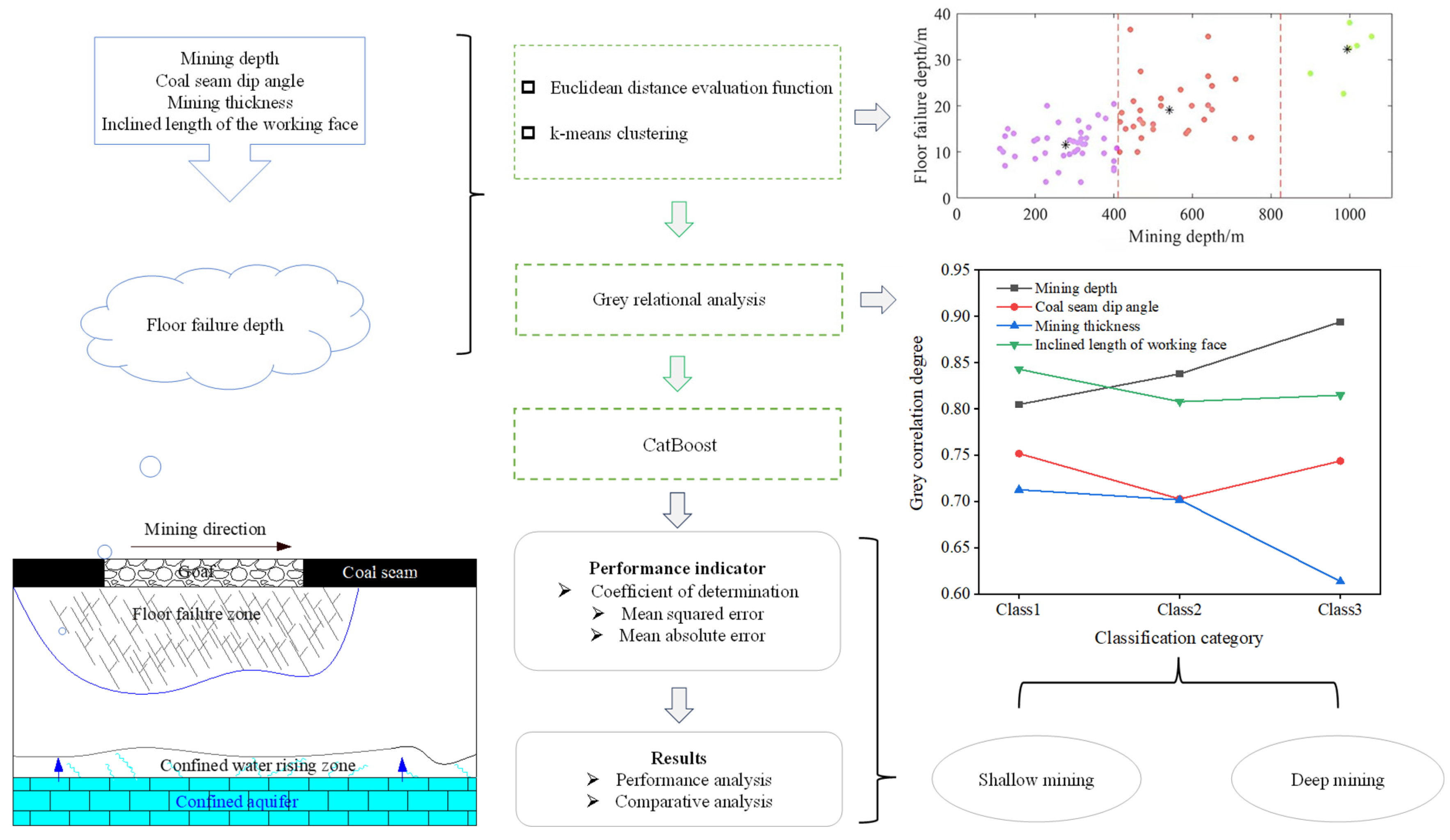
Prediction of Floor Failure Depth Based on Dividing Deep and Shallow Mining for Risk Assessment of Mine Water Inrush

by
Weitao Liu
1,2,
Mengke Han
1,* and
Jiyuan Zhao
1
1
College of Safety and Environmental Engineering, Shandong University of Science and Technology, Qingdao 266590, China
2
College of Energy and Mining Engineering, Shandong University of Science and Technology, Qingdao 266590, China
*
Author to whom correspondence should be addressed.
Water 2024, 16(19), 2786; https://doi.org/10.3390/w16192786
Submission received: 12 August 2024 / Revised: 21 September 2024 / Accepted: 26 September 2024 / Published: 30 September 2024

Abstract

:
Understanding and predicting floor failure depth is crucial for both mitigating mine water inrush hazards and safeguarding groundwater resources. Mining activities can significantly disturb the geological strata, leading to shifts and damage that may result in floor cracks. These disruptions can extend to confined aquifers, thereby increasing the risk of water inrushes. Such events not only pose a threat to the safety of mining operations but also jeopardize the sustainability of surrounding groundwater systems. Therefore, accurately predicting floor failure depth to take effective coal seam floor management measures is the key to reducing the impact of coal seam mining on water resources. Seventy-eight sets of data on coal seam floor failure depth in China were collected, and the main controlling factors were considered: mining depth (D1), working face inclination length (D2), coal seam inclination (D3), and mining thickness (D4). Firstly, the distance evaluation function based on Euclidean distance was constructed as the clustering effectiveness index, and the optimal cluster number K = 3 was determined. The collected data were clustered into three categories using the K-means clustering algorithm. It was found that the clustering results were positively correlated with the size of D1, indicating that D1 played a dominant role in the clustering. The D1 dividing points of the three types of samples were between 407.7~414.9 m and 750~900 m. On this basis, the grey correlation analysis method was used to analyze the order of the influence weights of the main controlling factors of coal seam floor failure depth. For the first group, the order was D2 > D1 > D3 > D4, while, in the other two, it was D1 > D2 > D3 > D4. D1 emerged as the most influential factor, surpassing D2. Therefore, D1 between 407.7 and 414.9 m could be used as the boundary, the first group could be classified as shallow mining, and the second and third groups could be classified as deep mining. Based on this boundary, CatBoost prediction models for the depth of coal seam floor failure in deep and shallow parts were constructed and the prediction results of the model test set were compared with the calculation results of the empirical formula. These models exhibited superior accuracy with a lower mean squared error (MSE) and mean absolute error (MAE) and a higher R-squared (R2) compared to the empirical formula. This study helps to enhance the understanding of coal seam floor behavior, guide floor management, and protect groundwater resources by defining deep and shallow mining to accurately predict floor failure depth.

1. Introduction

Coal seam mining causes the coal seam floor to experience pressure relief, leading to mechanical damage and the formation of a floor failure zone at a specific depth. Coal seam failure can be defined as the mechanical disruption and deformation of the rock mass beneath the coal seam, resulting from the stress redistribution that occurs during mining. This failure may extend into underlying aquifers, affecting groundwater quality and hydrodynamics. If it affects the underlying aquifers, it may impact the quality of groundwater through the presence of organic matter within mineral resources, resulting in deteriorating water quality and altering the relationship between water recharge, runoff, and discharge [1,2,3,4,5,6]. This change has far-reaching impacts on both the water supply source in the mining area and its surrounding areas. Studying the law of mine floor failure and predicting the failure depth so as to take effective floor management measures are beneficial in reducing adverse effects on water resources.
As the mining depth increases, the mechanical failure characteristics of the coal seam floor rock mass will change, transforming from elasticity to plasticity and showing a certain degree of ductility [7]. Therefore, in order to study the failure characteristics of coal seam floors at different depths and accurately predict the failure depth, it is necessary to clarify how to first divide the deep and shallow portions and how to divide deep and shallow mining. Xie et al. [8] believed that the definition of “deep” is essentially a mechanical problem that needs to be determined by considering the stress state, stress level, and original rock properties. The concepts and definitions of subcritical depth, critical depth, and supercritical depth were proposed to determine whether a coal mine enters the phase of deep mining and provide quantitative indicators. Xie et al. [9] also analyzed the increasing occurrence of a series of engineering disasters such as rock bursts, coal and gas outbursts, roof collapses, and floor water inflows caused by the increase in mining depth and elucidated the quantitative boundary between deep and shallow differences both domestically and internationally. Qian [10] proposed defining deep rock mass engineering based on the phenomenon of zonal disintegration. He [11] and He et al. [12] proposed defining the depth of deep mining as the depth at which nonlinear mechanical phenomena first appear in the engineering rock mass. Zhang et al. [13] established criteria and methods for defining deep coal mining based on the quasi-hydrostatic pressure environment in shallow crusts and coal mining areas in China. There are various opinions regarding the definition of deep and shallow mining, and no clear boundary exists. As a result, the methods for comparing and analyzing the failure characteristics of deep and shallow coal seam floors, establishing boundaries for deep and shallow mining, and predicting the failure depth of coal seam floors at different depths vary and include, for example, theoretical calculation methods, empirical formula methods, similar simulation methods, numerical simulation methods, on-site measurement methods, etc. Xu and Yang [14] derived a statistical formula for floor failure depth under the condition of large buried depth by analyzing the measured results of 21 floor failure depths with the burial depth exceeding 400 m, while Liu et al. [15] developed a calculation formula for mine floor failure depth based on the semi-infinite body theory and the Mohr–Coulomb failure criterion. Dong et al. [16] utilized MATLAB R2018a to perform regression analysis using numerical simulations and relevant measured data. They established a fitting equation that takes into account the dip length, mining depth, and mining height of the working face. Hu et al. [17] developed a multivariate regression analysis model for the prognostication of deep mine floor failure depth. They analyzed field-measured data from 39 floor failure depths, all exceeding 400 m, in the eastern mining region of the North China Coalfield. The above-mentioned studies provide guidance for the definition of deep and shallow mining and the prediction of floor failure depth. However, these methods often suffer from slow processing speeds due to complex calculations or large-scale numerical simulations. At the 175th Xiangshan Conference in 2002 [18], the experts and scholars in attendance believed that the theory and technology of deep mining should not be confined to the current concepts and technical levels. They advocated for forward-thinking, the development of new mining technologies, and the advancement of mining technology as a whole. Hence, simple and efficient machine learning algorithms across disciplines can be employed to divide deep and shallow mining and predict the depth of floor failure.
Machine learning (ML) algorithms excel at analyzing vast datasets, detecting intricate patterns, and drawing meaningful conclusions. They are currently being applied across diverse research domains, yielding promising results. Davoodi et al. [19] used a variety of machine learning algorithms to predict uniaxial compressive strength based on drilling variables. De Gouveia et al. [20] employed machine learning to classify emergency shutdown valve damage. Furthermore, machine learning finds valuable applications in predicting reservoir landslide displacement [21], lithology [22], and water environments [23,24].
Therefore, leveraging the benefits of machine learning to process data efficiently and accurately, in this study, the K-means clustering algorithm in machine learning and the CatBoost algorithm for regression prediction are introduced into the field of coal mining. Utilizing measured data on coal seam floor failure depths in China and considering the variation in the failure patterns of coal seam floors at different depths, a distance evaluation function based on Euclidean distance was applied to ascertain the optimal number of clusters and conduct K-means clustering. This aimed to partition the measured data based on variations in mining depth. Subsequently, the grey correlation analysis method was applied to elucidate the degree of correlation between the failure depth of coal seam floors at different depths and their main controlling factors. This process helped establish the boundary between deep and shallow mining. The CatBoost model for predicting the failure depth of deep and shallow coal seam floors was constructed using data on the failure depths of these floors. Subsequently, the floor’s failure depth was accurately predicted (Figure 1).
The primary objective of this study was to predict the floor failure depth of coal seams based on the division of deep and shallow mining. Specifically, this study aimed to (1) define the boundary between deep and shallow mining through data clustering and correlation analysis and (2) develop a predictive model using the CatBoost algorithm to estimate the failure depth of coal seam floors. By leveraging machine learning methods, this study aimed to provide a more efficient and accurate approach to predicting floor failure depth, which can assist in mitigating the adverse impacts on water resources caused by coal mining and contribute to better risk assessment and management of mine water inrush.

2. Basic Data on Coal Seam Floor Failure Depth

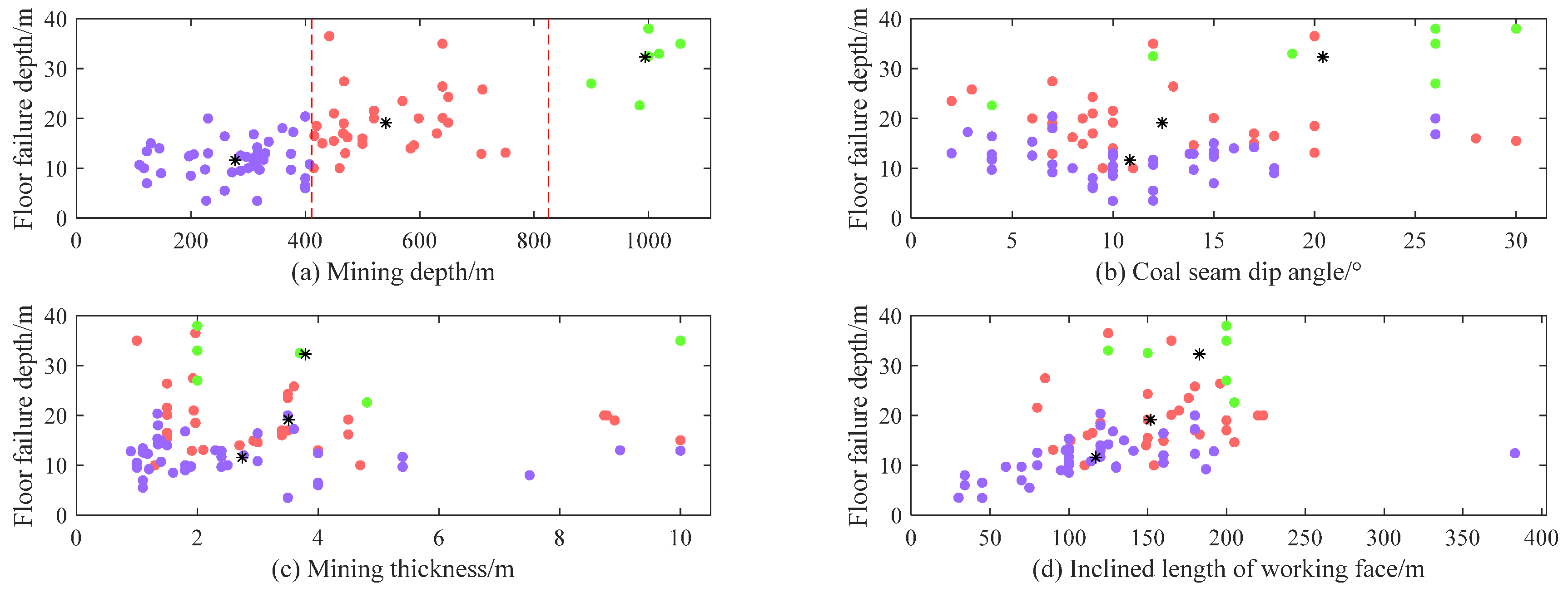
2.1. Analysis of the Main Controlling Factors

The failure of a coal seam floor results from a multitude of complex factors. Therefore, based on previous research findings [25,26,27], four main controlling factors were chosen for consideration. These factors included mining depth (D1), inclined length of the working face (D2), coal seam dip angle (D3), and mining thickness (D4). Although the anti-failure ability of the floor and the geological structure of the coal seam floor can also influence the extent of floor failure, these are relatively qualitative variables, and the corresponding amount of information is not fully reflected in calculations of floor failure depth. Therefore, they were not considered. (1) D1 is a key factor influencing the original rock stress field in mine rock masses. The magnitude of the original rock stress is positively correlated with D1. As D1 increases, the amplitude and intensity of stress changes in the coal seam floor before and after mining gradually increase, thereby increasing the floor failure depth. (2) D2 is positively correlated with floor failure depth in a coal seam within a certain range. As D2 increases, the range of mining influence expands, and, under the mining pressure, the deformation range of the floor rock mass towards the goaf increases, thereby leading to an increase in floor failure depth. (3) The variation in D3 changes the degree and area of stress concentration within the floor, thereby altering the failure depth of a coal seam floor. (4) As D4 increases, the periodic weighting step of the working face becomes larger, leading to greater mine pressure. This increased pressure causes greater settlement displacement in the surrounding rock, which, in turn, deepens the floor failure. The intensified stress and deformation in the rock strata result in a deeper and more pronounced failure of the mine floor.

2.2. Statistical Analysis of Measured Data

Building on the analysis above, a study on floor failure depth under the influence of D1, D2, D3, and D4 was conducted. Measured data on the floor failure depth from various mining areas in China [28,29,30,31,32] were gathered and organized based on D1 (Table 1 and Table S1).
Table S1 reveals that, on the whole, floor failure depth increases with rising D1. Nevertheless, due to the influence of other main controlling factors, its law exhibits some degree of instability [26]. Consequently, we could conduct further research to divide the boundary between deep and shallow regions by examining the distinct variation characteristics in the failure behavior of coal seam floors at varying depths.

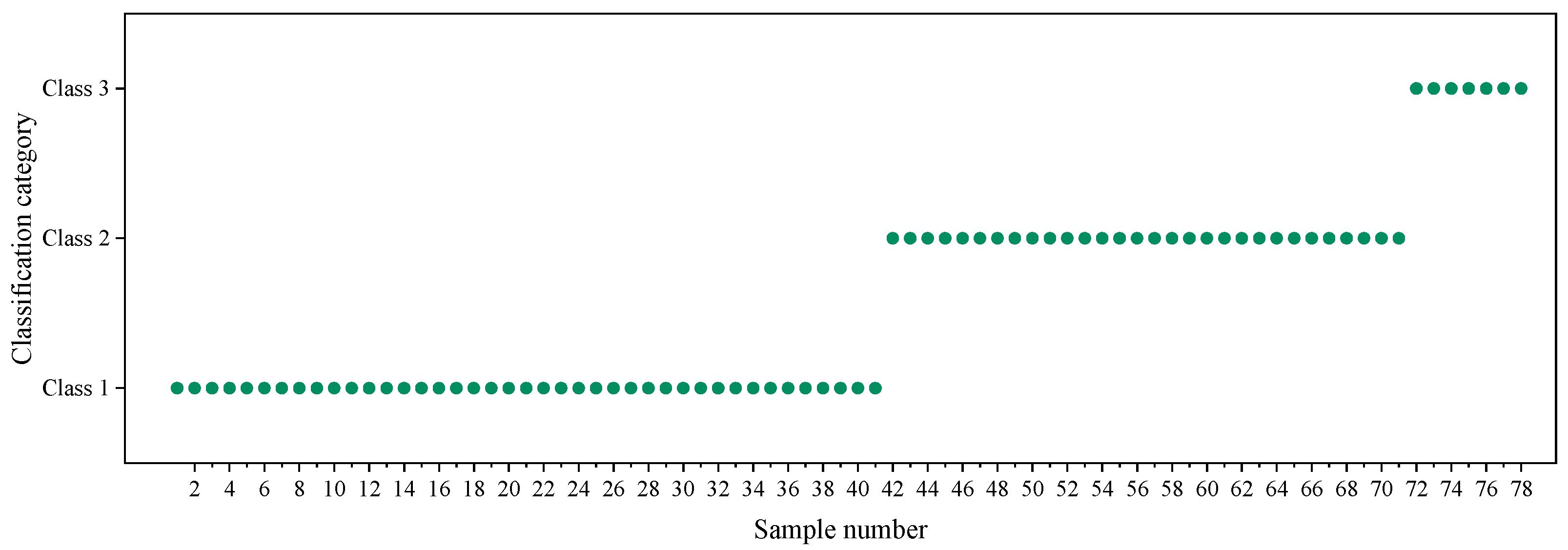
3. Cluster Analysis of Measured Data Based on Different Mining Depths

As D1 increases, the stress state of coal seam floor strata undergoes some degree of alteration. As a result, this alteration results in changes in the correlation between the floor failure depth and its main control factors. In other words, the internal relationship between the independent variable (the main controlling factor) and the dependent variable (floor failure depth) will shift. According to the phenomenon of differences in the failure patterns of coal seam floors at different depths, can D1 be considered a parameter to classify the measured data of coal seam floor failure depths? To test this hypothesis, a distance-based K-means clustering algorithm was applied, which categorized data samples into different groups based on their similarity. Therefore, by utilizing the measured data from Table S1 concerning the coal seam floor’s failure depth, the optimal clustering number could be identified and used for clustering. This allowed for the classification of the measured data in accordance with changes in D1.

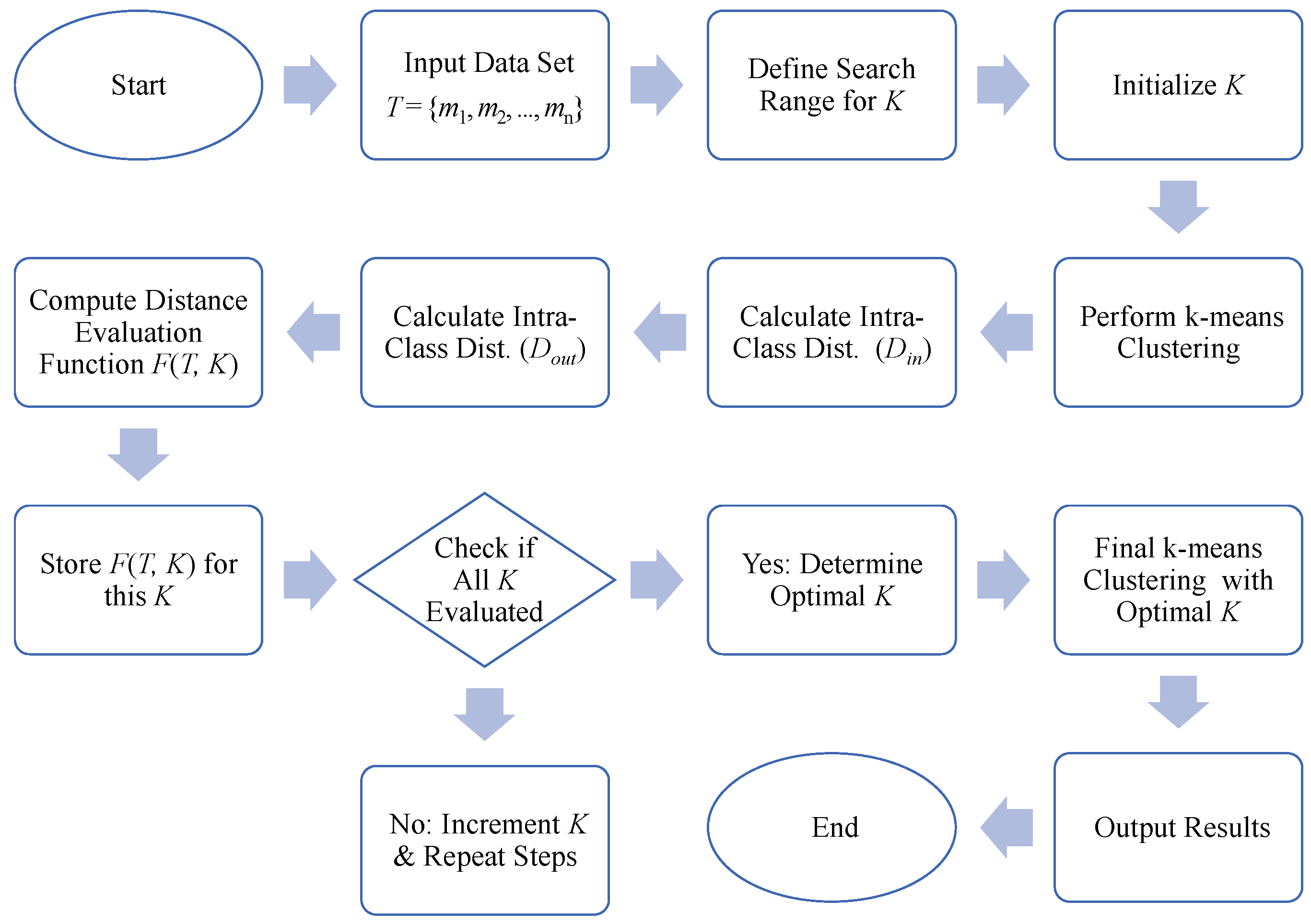
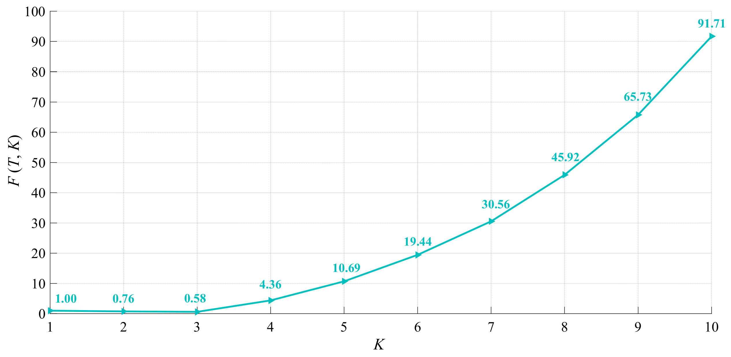
3.1. Selection of the Optimal Number of K Clusters

The K-means clustering algorithm is an efficient, simple, and flexible method [33]. Because the calculation amount is relatively small, it is suitable for small sample datasets. However, choosing an appropriate clustering (K value) can be difficult with small sample datasets because the number of data points is limited, and an incorrect selection of the K value can lead to over-clustering or under-clustering problems. To reasonably categorize the measured data, it is essential to determine the optimal clustering number. The basic algorithm for determining the optimal K-means cluster includes the following steps (Figure 2): Define a search range for a specific dataset, containing potential values of K (cluster numbers). Perform the K-means clustering algorithm to generate clustering results for various K values. Select the appropriate validity index to evaluate the quality of the clustering results and thus determine the optimal cluster based on the evaluation results. In general, an effective clustering partition should strive to accurately represent the internal structure of the dataset, making the samples within each cluster as similar as possible while maximizing dissimilarity between clusters. From a distance perspective, this entails minimizing the algebraic sum of intra-class distances and maximizing the algebraic sum of inter-class distances, with the corresponding cluster number being the optimal choice. To adhere to this fundamental principle, a distance evaluation function grounded in Euclidean distance was formulated as a clustering validity index [34]. This index served to assess the clustering performance of the K-means algorithm and identify the most suitable cluster number, denoted as K. Using the distance evaluation function based on Euclidean distance to select the optimal number of K clusters offers several advantages. First, Euclidean distance provides a simple and intuitive way to measure similarity, helping to minimize intra-cluster distances and maximize inter-cluster distances. This ensures well-separated and coherent clusters. Additionally, by balancing these distances, the distance evaluation function systematically determines the optimal K by minimizing errors, avoiding arbitrary selection and improving clustering accuracy.
Following the general principles of spatial clustering algorithms, the classification process should maximize the internal similarity within the same class while minimizing differences and simultaneously minimize the similarity between classes while maximizing differences. In other words, the distance between any spatial object and the center of its corresponding class should be smaller than the distance between the object and the geometric center of any other class. Only then does the clustering criterion function converge:
E = i = 1 k p C i ( p m i ) 2
where E is the sum of squares of the errors of all research objects, p is the research data object, and mi is the average value of class Ci.
Building upon the fundamental concepts outlined above, a distance evaluation function was formulated and the optimal cluster number K was ascertained by minimizing this distance evaluation function as follows.
Assume the research sample dataset: T= {m1, m2, …, mn}, and the number of clusters is K.
(1)
Consider I = {T, K} as the clustering space and define the inter-class distance as the summation of Euclidean distances from all cluster centers (the mean of samples within each class) to the center of the universe (the mean of all samples):
D o u t = i = 1 k m i m 2
where Dout is the distance between classes, m is the sample mean, and mi is the mean of all samples in class Ci.
(2)
Consider I = {T, K} as the clustering space. Intra-class distance is defined as the summation of internal distances within all classes. More specifically, intra-class distance is calculated as the sum of the Euclidean distances from all objects within each class to the respective class center:
D i n = i = 1 k p C i p m i 2
where Din is the intra-class distance, p is any spatial object, and mi is the mean of all samples in class Ci.
(3)
Consider I = {T, K} as the cluster space. When Dout is approximately equal to Din, this indicates that the number of clusters is optimal. Consequently, the distance evaluation function is defined as follows:
F ( T , K ) = D o u t D i n 1
When using the distance evaluation function as the clustering validity test function, since the sum of inter-class distances Dout is a monotonic increasing function of the cluster number K and the sum of intra-class distances Din is a monotonic decreasing function of the cluster number K, the distance evaluation function determined by Equation (4) must have a minimum point. The result of spatial clustering is optimal when the distance evaluation function hits its minimum; hence, the best value for K is as follows:
Min i { F ( T , K ) } ( K = 1 , 2 , 3 , , n )
Based on the measured data, cluster numbers K ranging from 2 to 10 were considered. Subsequently, utilizing MATLAB R2018a, the distance evaluation function was programmed, and the corresponding F (T, K) values for different cluster numbers K were acquired, as illustrated in Figure 3. In accordance with Equation (5), it was determined that the optimal cluster number was K = 3.

3.2. Determination of Cluster Category

The K-means clustering algorithm [35] is an iterative clustering analysis algorithm. The specific steps are outlined as follows:
(1)
Determine the number of clusters, K. Establish the optimal number for dividing the dataset. As per Section 3.1, the most suitable cluster number was K = 3.
(2)
Cluster center initialization: K data points are randomly chosen from the dataset to serve as the initial cluster centers:
C ( 0 ) = { c 1 ( 0 ) , c 2 ( 0 ) , , c k ( 0 ) }
where C ( 0 ) represents the initial cluster center set and c j ( 0 ) represents the initial j-th cluster center.
(3)
Assign data points to cluster centers:
S i = { j d ( x i , c j ( t ) ) d ( x i , c l ( t ) ) , l j }
where Si denotes the index set of the cluster to which the i-th data point belongs, d ( x i , c j ( t ) ) signifies the distance between the data point xi and the j-th cluster center c j ( t ) , and c l ( t ) represents the l-th cluster center at the t-th iteration.
(4)
Update the cluster centers:
c j ( t + 1 ) = 1 | S j | i S j x i
where c j ( t + 1 ) represents the updated position of the j-th cluster center and | S j | represents the number of data points belonging to the j-th cluster.
(5)
Iterate through steps 3 and 4 until the cluster center positions remain unchanged or a predefined number of iterations is reached.
(6)
Upon completion of clustering, assign each data point to a cluster.
The cluster number was set at K = 3. Using MATLAB R2018a, the measured data underwent clustering and analysis. The resulting clustering outcomes were arranged according to the sample numbers shown in Table S1, and these results are illustrated in Figure 4.
Figure 4 reveals that during K-means clustering, the clustering results exhibited a clear positive correlation with D1, indicating that D1 had a significant impact on the clustering outcomes. This suggested that D1 played a dominant role in clustering and had a substantial influence on the final clustering results.
To further validate this, scatter plots illustrating the relationship between the main controlling factors and the depth of floor failure were generated (Figure 5). Each subplot portrays the connection between a main controlling factor and the depth of floor damage. Consistent with the clustering results in Figure 4, the data points are color-coded, with each color representing a distinct cluster. The black asterisk denotes the cluster center.
These scatter plots provide insights into the relationship between various main controlling factors and the depth of floor failure, as well as the partitioning effect of the clustering algorithm on the measured data. Figure 5a reveals that clustering patterns changed with D1, indicating a clear division. Figure 5b–d demonstrate that the floor failure depth did not exhibit regular clustering patterns when varying D3, D4, and D2. Based on changes in D1, measured data could be categorized into three groups, reflecting differences in floor failure behavior at different depths. Based on the clustering results, the first category comprised samples numbered 1 to 41, the second category included samples numbered 42 to 71, and the third category comprised samples numbered 72 to 78. Similar sample data exhibited strong similarities, and coal seam floor failure followed similar patterns within each category. The demarcation points between these three sample groups were between 407.7 to 414.9 m and 750 to 900 m, respectively. As the sample size of measured data increased, this method allowed for classification based on different mining depths more accurately.

4. Grey Correlation Analysis of the Main Controlling Factors in Deep and Shallow Coal Seams

The determination of the clustering results of the measured data served as a foundation for elucidating the differences in the failure patterns of coal seam floors at different depths. Subsequently, the grey correlation analysis method was employed to investigate the correlation between the coal seam floor failure depths of the three types of samples and their main controlling factors.

4.1. Grey Relational Degree Theory

The grey correlation degree [36,37] is a method used to quantitatively characterize the degree of correlation among factors. The relationship between D1, D2, D3, and D4 (comparison sequence) and floor failure depth (reference sequence) was analyzed using the grey relational analysis method and quantitatively described.

4.2. Grey Relational Grade Calculation

(1)
Average dimensionless processing
In order to compare the correlation degree of different dimensions, these sequences needed to be averaged and made dimensionless first, that is,
X i ( k ) = x i ( k ) x ¯
where xi(k) is the original sequence, x0(k) is the reference sequence when i = 0, and xi(k) is the comparison sequence when i = 1, …, n. xi(k) is the data sequence after mean processing, k is the number of indicators, and x ¯ is the average of the original sequence.
(2)
Calculation of the correlation coefficient
ξ i ( k ) = min i min k | X 0 ( k ) X i ( k ) | | X 0 ( k ) X i ( k ) | + ρ max i max k | X 0 ( k ) X i ( k ) | + ρ max i max k | X 0 ( k ) X i ( k ) | | X 0 ( k ) X i ( k ) | + ρ max i max k | X 0 ( k ) X i ( k ) |
where ρ is the resolution coefficient, which was taken as 0.5; ξ i ( k ) represents the correlation coefficient between the k-th index parameter of the i-th comparison sequence and the k-th index parameter of the reference sequence.
(3)
Grey relational degree solution
The solution for the grey correlation degree involved calculating the average value of the correlation coefficient across each comparison sequence, that is,
R i = 1 m k = 1 m ξ i ( k )

4.3. Grey Relational Analysis

To accurately analyze the correlation between each main controlling factor and floor failure depth, we conducted grey correlation analysis on three types of samples (Figure 6).
As shown in Figure 6, the grey correlation degree was utilized to evaluate the influence of different mining parameters on floor failure depth. The grey correlation degree quantified the relationship between influencing factors and floor failure depth. A higher grey correlation degree indicated a stronger influence of the factor on floor failure depth, suggesting that adjustments in this parameter could significantly impact mining safety and operational decisions. Conversely, a lower grey correlation degree suggested a weaker influence, indicating that changes in this parameter might have less of an impact on floor failure depth under current mining conditions.
From Figure 6, it is discernible that as D1 increased, the correlation between D2, D4, and floor failure depth exhibited a downward trend. In contrast, the correlation between D3 and floor failure depth initially decreased and then rose, while the correlation between D1 and floor failure depth remained consistently high and demonstrated an upward trend. The boundary of D1 between Class 1 and Class 2 in Figure 6 was within the range of 407.7 to 414.9 m. The values 407.7 m and 414.9 m were determined through the clustering analysis of the measured data, as discussed earlier. During the transition from 407.7 m to 414.9 m in D1, it gradually surpassed D2 as the first influencing factor affecting floor failure depth, and this influence continued to grow. From the above analysis, it can be seen that with the gradual extension of the coal seam to more depth, among the four main controlling factors, only the correlation between D1 and floor failure depth gradually increased. The order of influence weights for each main controlling factor on the floor failure depth of the first type of sample was as follows: D2 > D1 > D3 > D4. For the second and third types of samples, the order of influence weights on floor failure depth was D1 > D2 > D3 > D4. Hence, D1 between 407.7 m and 414.9 m could be considered the boundary, categorizing the first type of sample as shallow mining and the second and third types as deep mining. This is generally consistent with the conclusions of previous studies [14,17,29,38]. When comparing the weight order of the main controlling factors on floor failure depth, we can see that the floor failure depth of shallow coal seams was most affected by D2, while the floor failure depth of deep coal seams was most affected by D1.
Through a comparison of the grey relational analysis, it became evident that the primary controlling factor for deep coal seam floor failure was D1, primarily manifesting in the alteration of the original rock stress. As D1 increased, the deep coal seam floor experienced high in situ stress. After coal seam mining, the vertical stress exerted on the coal seam floor rapidly dissipated, resulting in the alleviation of pressure on the floor rock mass and the release of surplus energy. This process promoted the expansion of floor failure depth [29,39]. Hence, as mining continued to extend to greater depths, D1 progressively superseded D2 and became the primary factor influencing the depth of coal seam floor failure.

5. Prediction of Floor Failure Depth in Deep and Shallow Coal Seams

Due to the rapid advancement of artificial intelligence, machine learning algorithms for regression prediction are continuously evolving and improving. The prediction of floor failure depth is inherently complex and filled with uncertainties, involving various geological, engineering, and environmental factors. The interactions among these factors necessitate that prediction models be capable of processing a vast amount of nonlinear, unstructured data and strong interactions between variables. In this context, the CatBoost algorithm, with its advanced numerical feature handling, efficient data fitting capabilities, and superior generalization performance, significantly enhances the accuracy and reliability of predictions for floor failure depth. These advantages make CatBoost an ideal choice for addressing such complex prediction problems. Therefore, this study used the CatBoost algorithm to establish floor failure depth prediction models. To assess the influence of categorizing measured data into deep and shallow categories on the predictive performance of the model, this section establishes prediction models for two types of data for comparison: deep coal seam floor failure depth data and shallow coal seam floor failure depth data. Lastly, we compare the predictive performance of the empirical formula from the “Guide to Coal Pillar Setting and Coal Pressing Mining for Buildings, Water Bodies, Railways, and Main Roadways” [28] with the CatBoost prediction models established for deep and shallow mining categories.

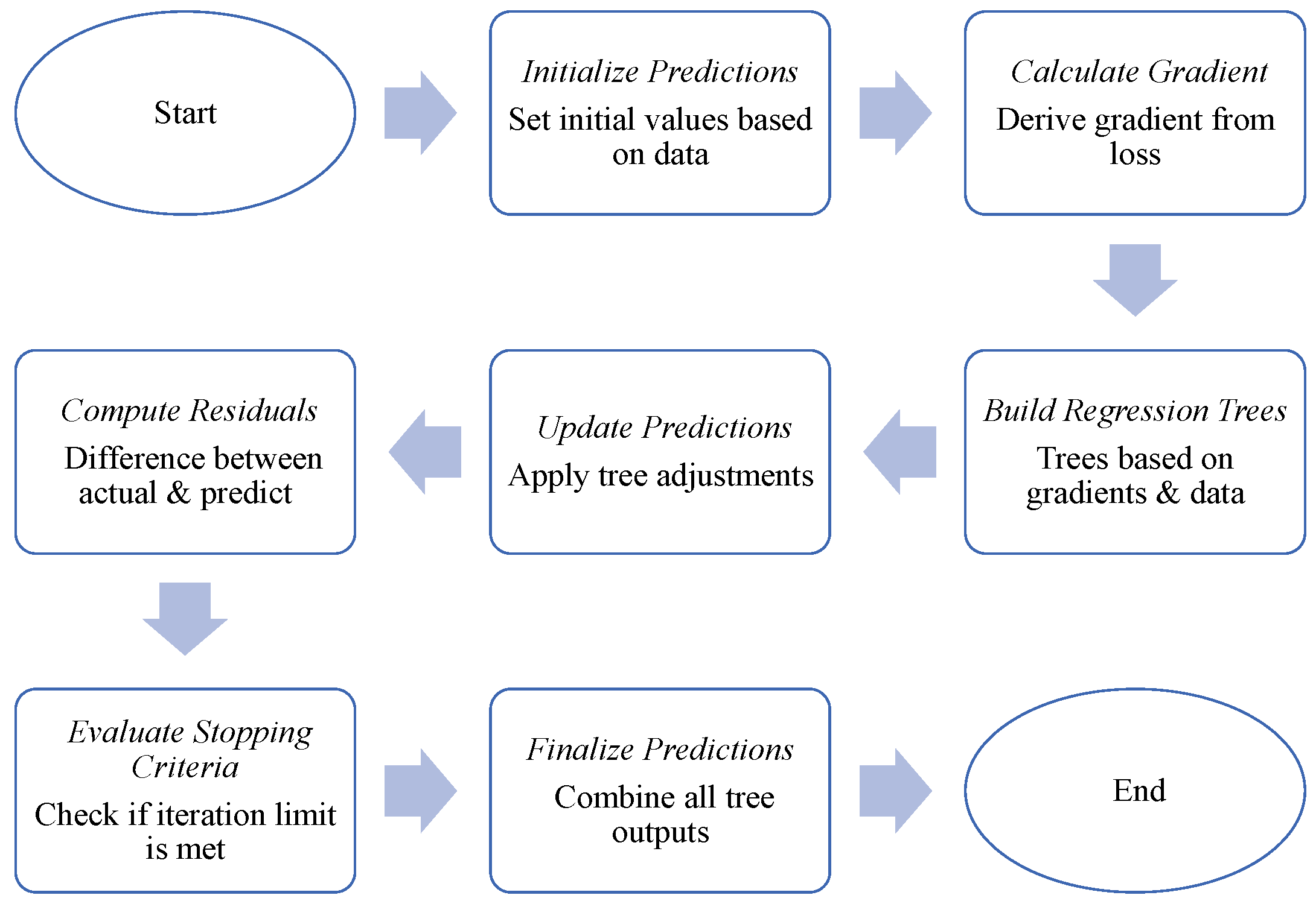
5.1. Principles of the Catboost Algorithm

CatBoost [40,41] is a gradient-boosting decision tree (GBDT) framework based on symmetric decision trees. This is a widely used machine learning algorithm. CatBoost can yield excellent results with relatively small datasets, unlike deep learning (DL) models that require extensive data for training [42]. CatBoost addresses concerns such as gradient bias, prediction shift, and overfitting and improves the accuracy and generalization capabilities of the algorithm. Therefore, CatBoost can be applied to tackle regression problems. The specific steps are outlined below (Figure 7):
(1)
Initialization: Specify the number of iterations (T) and the learning rate (η). Initialize the model’s predicted value (p), typically by using the average value of the training set. Assuming there are n samples in the training set, the initial prediction value is
p i 0 = 1 n i = 1 n y i
where yi represents the actual value of the i-th sample.
(2)
Calculate the gradient of the loss function: Compute the gradient of the loss function for each sample with respect to the current model’s predicted value. In the case of regression problems, the loss function employs the squared loss function (L2 loss):
L ( y i , p i ) = ( y i p i ) 2
(3)
Build regression trees: In each iteration, construct a regression tree based on the gradient of the loss function and the information gain of features. A regression tree is a decision tree designed for gradient boosting and is used to model regression problems.
(4)
Update the model’s prediction value: Adjust the model’s prediction value based on the currently constructed regression tree. For the t-th iteration (t = 1, 2, …, T), the updated predicted value is
p i t = p i ( t 1 ) + η f t ( x i )
where ft(xi) represents the predicted value of the regression tree for the sample xi in the t-th round iteration.
(5)
Update residuals: Compute the difference between the current predicted value and the actual label to obtain the residual for the next iteration. For the t-th round of iteration, the calculated residual is
r i t = y i p i t
(6)
Check stopping criteria: Check whether the predefined number of iterations T has been reached or if other stopping criteria (e.g., error convergence) have been met. If the stop criterion is satisfied, the training process concludes; otherwise, it returns to step 3.
(7)
Conduct final prediction: Once the training is finished, use CatBoost to aggregate the prediction outputs from all regression trees to produce the final model prediction result.
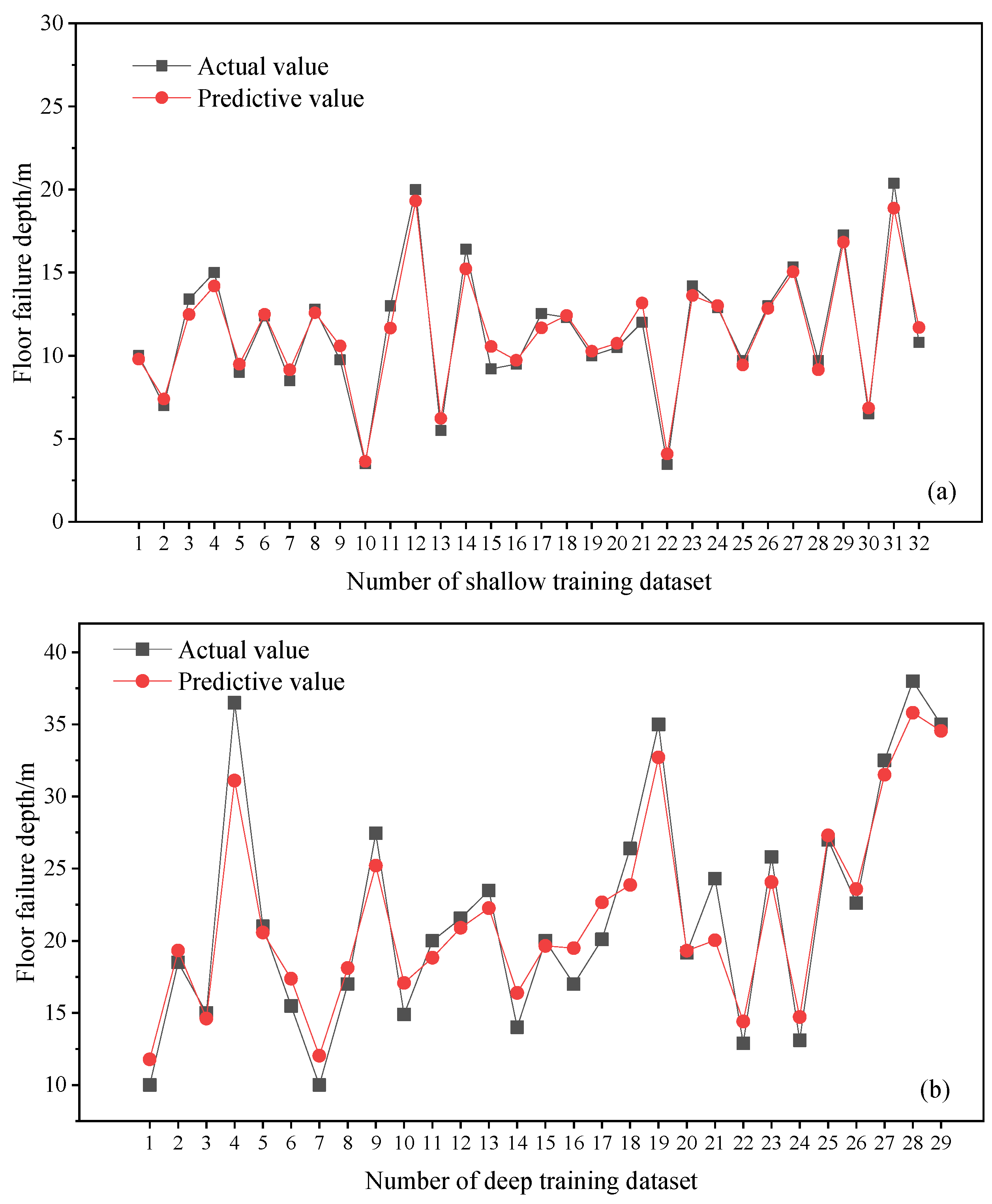
In general, the CatBoost algorithm constructs multiple regression trees iteratively, persistently optimizing the model’s predicted values through gradient boosting to effectively address regression problems and minimize squared loss. This design equips CatBoost with high accuracy and strong generalization capabilities for regression problems.

5.2. Modeling

Building upon the preceding analysis, D1 values between 407.7 m and 414.9 m were used as a threshold to categorize the first type of sample as shallow mining, while the second and third types were classified as deep mining. As a result, sample data numbered 1 to 41 in Table S1 were utilized as the foundational data for predicting shallow coal seam floor failure depth, while sample data numbered 42 to 78 were used for predicting deep coal seam floor failure depth. For these two models, the input variables consisted of D1, D2, D3, and D4. The output variable was the floor failure depth. The sample data were divided into training and testing sets at a ratio of 8:2 for model construction, following the guidelines suggested in Professor Zhou’s “Machine Learning” [43]. After the division for predicting shallow coal seam floor failure depth, the training set comprised 32 data groups, while the testing set comprised 9 data groups. The shallow test set data are numbered 1, 6, 24, 29, 30, 33, 35, 37, and 39 in Table S1. After the division for predicting deep coal seam floor failure depth, the training set contained 29 data groups and the testing set contained 8 data groups. The deep test set data are numbered 43, 51, 53, 54, 56, 61, 76, and 77 in Table S1. The CatBoost model was configured with a maximum tree depth of 4, a learning rate of 0.05, and 200 iterations.

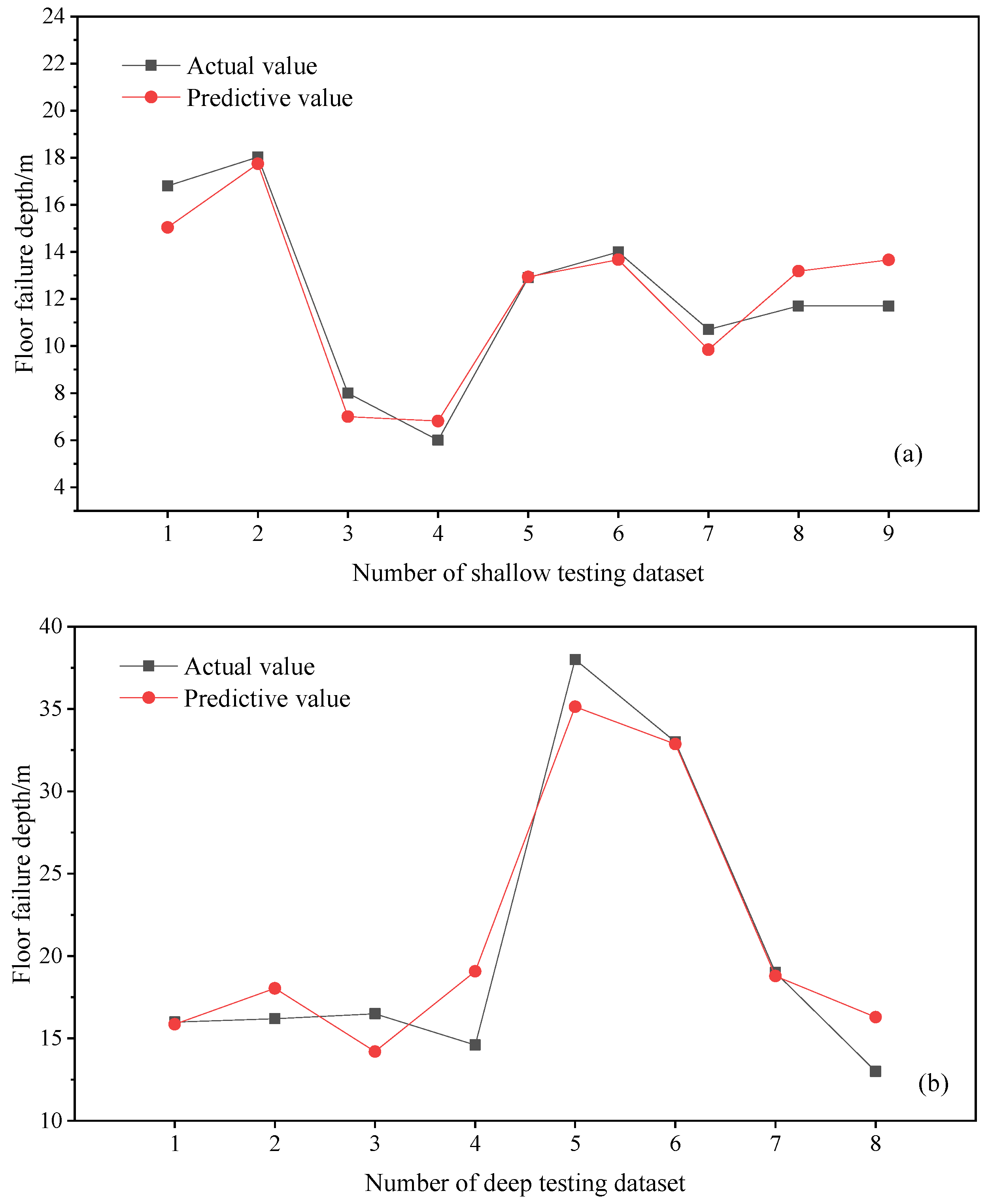
5.3. Model Evaluation

The CatBoost algorithm was employed to train and test the depths of failure in deep and shallow coal seams. MSE, MAE, and R2 were used to evaluate the model. MSE measures the average of the squares of the errors, which are the differences between predicted and actual values. A lower MSE indicates a model that predicts the data with higher accuracy. MAE measures the average of the absolute differences between predicted and actual values. A lower MAE points to a model that predicts more accurately. R2 is a statistical measure that represents the proportion of the variance for a dependent variable that is explained by an independent variable or variables in a regression model. A higher R2 value indicates that a model’s predictions are closer to actual data points, reflecting higher accuracy in the predictions. Figure 8 presents the performance analysis of the CatBoost prediction model for the training set. For the shallow training set, MSE = 0.50, MAE = 0.58, and R2 = 0.97. For the deep training set, MSE = 4.09, MAE = 1.66, and R2 = 0.93. It was obvious that the CatBoost models showed a good training effect, and the prediction results were in good agreement with the measurement results.
After the model training was completed, the CatBoost model was verified using the testing set. As illustrated in Figure 9, the performance of the CatBoost prediction model’s testing set was analyzed. For the shallow testing set, MSE = 1.30, MAE = 0.95, and R2 = 0.90. For the deep testing set, MSE = 6.00, MAE = 1.91, and R2 = 0.92. Despite the slightly larger MSE and MAE values for the testing set compared to the training set, the prediction accuracy for the testing set achieved a high level. The predicted values of the deep and shallow CatBoost models were basically consistent with the actual measured values. This showed that the deep and shallow CatBoost prediction models had good learning and prediction capabilities and could effectively predict floor failure depth.

5.4. Comparative Analysis of Prediction Results

To further demonstrate the robust predictive capability of the proposed models, the deep and shallow CatBoost prediction models were compared with the floor failure depth formula provided in the “Guide to Coal Pillar Setting and Coal Pressing Mining for Buildings, Water Bodies, Railways, and Main Roadways”. Using sample data from nine groups in the shallow testing sets and eight groups in the deep testing sets, shown in Figure 9, predictions for floor failure depth were generated. The analysis results are presented in Figure 10 and Table 2.
The formula for computing the depth of floor failure h was as follows:
h = 0.0085 H + 0.1665 α + 0.1079 L 4.3579
where H is D1, m; α is D3, °; and L is D2, m.
The MSE and MAE of the CatBoost prediction model for both the deep and shallow parts were lower than those of the empirical formula, and the R2 values were higher than those of the empirical formula. This indicated that the CatBoost prediction model had lower prediction errors and higher accuracy. Although empirical formulas are convenient for calculation, they consider fewer influencing factors, which may lead to significant deviations in predicting the depth of floor failure; in contrast, the CatBoost model, by analyzing a more comprehensive dataset and various variables, was able to provide more accurate predictions. The predicted values of the established deep and shallow CatBoost prediction models were basically consistent with the actual values, so they can be used to predict the depth of coal seam floor failure.

6. Discussion

The analytical prognostication of floor failure depth within coal mining contexts, as elucidated in this research, carries some implications for the stewardship of subterranean aquifer integrity. Given the critical role of precise predictions in floor failure phenomena, the findings facilitate the identification of zones susceptible to water inrush, which is of paramount importance for ensuring both mine safety and environmental conservation. The implications for aquifer protection are as follows: The improved ability to predict floor failure depths with greater accuracy enables the strategic placement of protective barriers and the adoption of specific excavation practices designed to minimize disturbances to water-bearing strata. Protecting these aquifers is crucial not just for preventing ecological damage but also for maintaining the water quality that local communities rely on. Preventive measures against water inrush may be as follows: Understanding the factors that influence floor failure helps us to act early to prevent water inrush events. Areas identified as high-risk may need changes in mining methods or the installation of advanced water control systems. For instance, by reducing the inclined length of the working face to control the area of the face, we can lower the chances of events that could lead to water inrush. Future research directions are as follows: There exists a pressing need for the refinement of predictive models concerning floor failure depth, with the incorporation of more influencing factors. Further scholarly inquiries into the enduring impacts of mining activities on aquifer dynamics are also imperative. These studies are expected to yield invaluable insights that could foster more sustainable mining practices.

7. Conclusions

Floor failure depth is an important indicator in the study of mine water inrush hazards and groundwater resource protection. The accurate prediction of floor failure depth is beneficial to the sustainability of groundwater. To minimize the adverse impact of coal seam mining on water resources, we collected 78 sets of coal seam floor failure depth data from China. We proposed and employed a range of efficient machine learning algorithms suitable for conducting in-depth research on small sample datasets. This study aimed to divide the boundaries of deep and shallow coal seam mining and provide accurate coal seam floor failure depth predictions. The primary findings are as follows:
(1)
First, using 78 sets of measured floor failure depth data and considering the differences in coal seam floor failure modes at different depths, a distance evaluation function based on Euclidean distance was formulated as a clustering effectiveness index. After employing this metric to identify the optimal number of clusters (K = 3), the K-means clustering algorithm was applied to categorize the data into three sample types. The D1 boundaries for these three sample types were within the range of 407.7 to 414.9 m and 750 to 900 m.
(2)
Subsequently, the grey correlation analysis method was used to calculate the correlation degree between the floor failure depth and its main controlling factors. The weight order for the first type of sample was as follows: D2 > D1 > D3 > D4. In the case of the second and third types of samples, D1 surpassed D2 and became the most influential factor. Therefore, taking the D1 range of 407.7 m to 414.9 m as the boundary, the first type of sample was categorized as shallow mining, while the second and third types were classified as deep mining. The determination of the mining boundaries of deep and shallow coal seams divided the measured data and provided basic data for the CatBoost prediction model for the depth of deep and shallow coal seam floor failure.
(3)
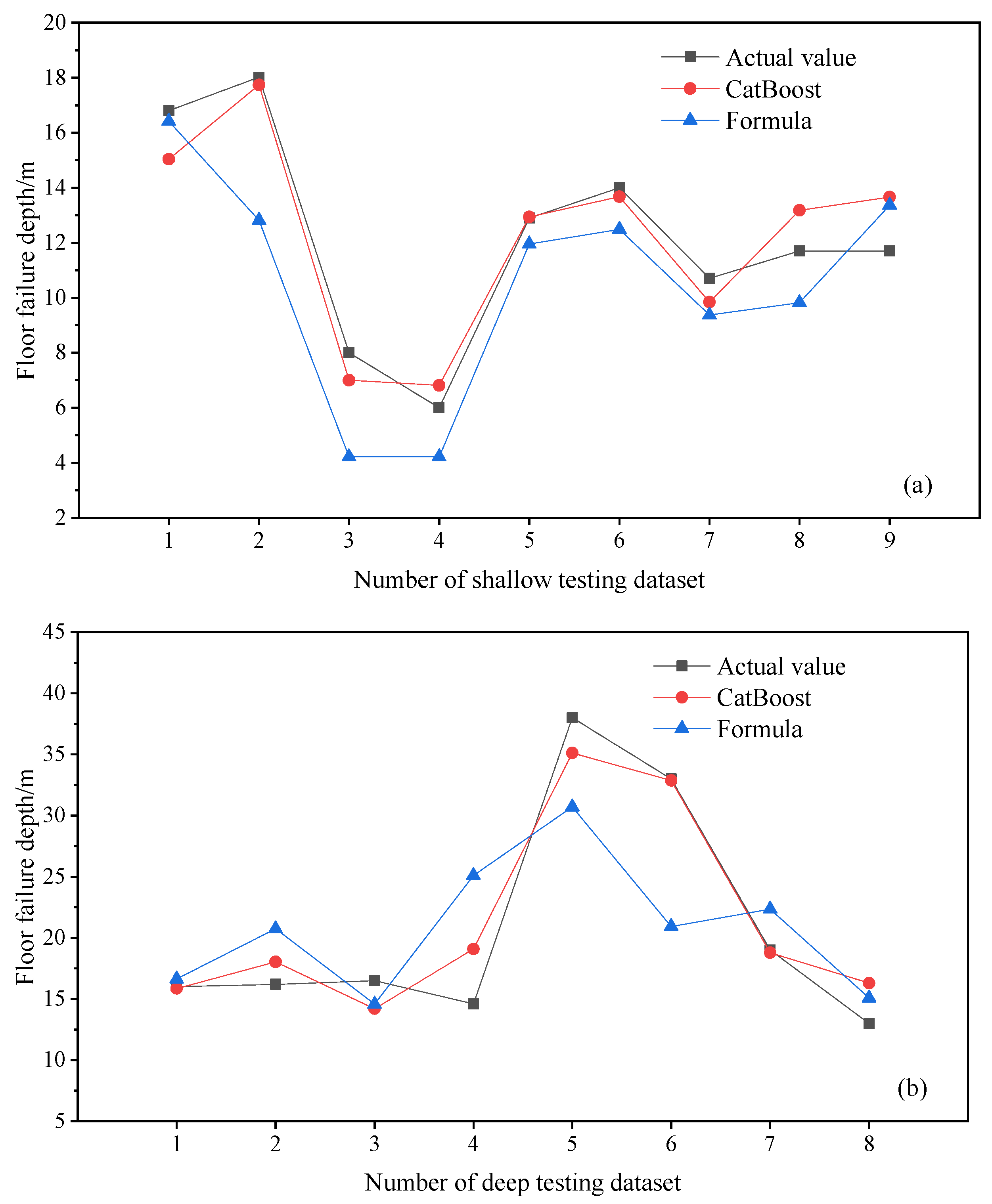
Finally, the CatBoost prediction model was trained and tested using the measured data of divided deep and shallow coal seam floor failure depths. For the training set of the shallow coal seam CatBoost prediction model, the MSE was 0.50, MAE was 0.58, and R2 was 0.97; for the testing set, the MSE was 1.30, MAE was 0.95, and R2 was 0.90. The training set of the deep coal seam CatBoost prediction model had MSE = 4.09, MAE = 1.66, and R2 = 0.93; the testing set had MSE = 6.00, MAE = 1.91, and R2 = 0.92. This shows that whether in the training set or the testing set, the predicted values generated by the CatBoost model were basically consistent with the actual values. In addition, through a comparative analysis between the CatBoost prediction models for deep and shallow parts and the empirical formula, it was found that the prediction accuracy of the CatBoost prediction models was better. For the shallow coal seam testing set, the empirical formula yielded MSE = 6.23, MAE = 2.06, and R2 = 0.52, while for the deep coal seam testing set, the empirical formula yielded MSE = 43.68, MAE = 5.30, and R2 = 0.43. In contrast, the CatBoost model for the shallow coal seam achieved MSE = 1.30, MAE = 0.95, and R2 = 0.90 and, for the deep coal seam, the CatBoost model yielded MSE = 6.00, MAE = 1.91, and R2 = 0.92. This comparison indicates that the CatBoost models for both deep and shallow parts were more accurate and effective in predicting the depth of floor failure.

8. Limitations and Recommendations

(1)
Due to the limited measured data collected, the D1 boundary divided by deep and shallow mining fell within a range. Therefore, more data need to be collected to enrich the dataset and narrow down the boundaries of subsequent deep and shallow mining.
(2)
Only four main controlling factors were considered, but, in the actual production process, there may be many factors that affect the depth of floor failure. In future studies, we hope to improve the model by taking into account as many factors as possible, such as the hard rock coefficient.

Supplementary Materials

The following supporting information can be downloaded at https://www.mdpi.com/article/10.3390/w16192786/s1: Table S1: Measured data of floor failure depth.

Author Contributions

Conceptualization, M.H.; methodology, M.H. and J.Z.; software, M.H. and J.Z.; validation, J.Z.; investigation, M.H.; data curation, M.H.; writing—original draft preparation, M.H. and J.Z.; writing—review and editing, W.L.; funding acquisition, W.L. and J.Z. All authors have read and agreed to the published version of the manuscript.

Funding

This research was funded by the Natural Science Foundation of Shandong Province, grant number ZR2023ME002, and the National Natural Science Foundation of China, grant number 52304238.

Data Availability Statement

The original contributions presented in this study are included in the article; further inquiries can be directed to the corresponding author.

Conflicts of Interest

The authors declare no conflicts of interest.

References

  1. Li, P.; Tian, R.; Xue, C.; Wu, J. Progress, opportunities, and key fields for groundwater quality research under the impacts of human activities in China with a special focus on western China. Environ. Sci. Pollut. Res. 2017, 24, 13224–13234. [Google Scholar] [CrossRef]
  2. Zhou, J.; Jiang, Z.; Qin, X.; Zhang, L. Heavy metal distribution and health risk assessment in groundwater and surface water of karst lead–Zinc Mine. Water 2024, 16, 2179. [Google Scholar] [CrossRef]
  3. Yin, D.; Lu, Z.; Li, Z.; Wang, C.; Li, X.; Hu, H. Effects of chloride ion transport characteristics and water pressure on mechanical properties of cemented coal gangue-fly ash backfill. Geomech. Eng. 2024, 38, 125–127. [Google Scholar] [CrossRef]
  4. Zipper, C.; Donovan, P.; Jones, J.; Li, J.; Price, J.; Stewart, R. Spatial and temporal relationships among watershed mining, water quality, and freshwater mussel status in an eastern USA river. Sci. Total Environ. 2016, 541, 603–615. [Google Scholar] [CrossRef] [PubMed]
  5. Moye, J.; Picard-Lesteven, T.; Zouhri, L.; El Amari, K.; Hibti, M.; Benkaddour, A. Groundwater assessment and environmental impact in the abandoned mine of Kettara (Morocco). Environ. Pollut. 2017, 231, 899–907. [Google Scholar] [CrossRef] [PubMed]
  6. Ren, Z.; Zhang, C.; Wang, Y.; Lan, S.; Liu, S. Stability analysis and grouting treatment of inclined shaft lining structure in water-rich strata: A case study. Geohaz. Mech. 2023, 1, 308–318. [Google Scholar] [CrossRef]
  7. Zhang, Z.; Xie, H.; Zhang, R.; Zhang, Z.; Gao, M.; Jia, Z.; Xie, J. Deformation damage and energy evolution characteristics of coal at different depths. Rock Mech. Rock Eng. 2019, 52, 1491–1503. [Google Scholar] [CrossRef]
  8. Xie, H.; Gao, F.; Ju, Y.; Gao, M.; Xie, L. Quantitative definition and investigation of deep mining. J. China Coal Soc. 2015, 40, 1–10. [Google Scholar]
  9. Xie, H.; Zhou, H.; Xue, D.; Wang, H.; Zhang, R.; Gao, F. Research and consideration on deep coal mining and critical mining depth. J. China Coal Soc. 2012, 37, 535–542. [Google Scholar]
  10. Qian, Q. The characteristic scientific phenomena of engineering response to deep rock mass and the implication of deepness. J. East China Inst. Technol. 2004, 27, 1–5. [Google Scholar]
  11. He, M. Conception system and evaluation indexes for deep engineering. Chin. J. Rock Mech. Eng. 2005, 24, 2854–2858. [Google Scholar]
  12. He, M.; Xie, H.; Peng, S.; Jiang, Y. Study on rock mechanics in deep mining engineering. Chin. J. Rock Mech. Eng. 2005, 24, 2803–2813. [Google Scholar]
  13. Zhang, J.; Li, Q.; Zhang, Y.; Cao, Z.; Wang, X. Definition of deep coal mining and response analysis. J. China Coal Soc. 2019, 44, 1314–1325. [Google Scholar]
  14. Xu, Y.; Yang, Y. Applicability analysis on statistical formula for failure depth of coal seam floor in deep mine. Coal Sci. Technol. 2013, 41, 129–132. [Google Scholar]
  15. Liu, W.; Mu, D.; Xie, X.; Yang, L.; Wang, D. Sensitivity analysis of the main factors controlling floor failure depth and a risk evaluation of floor water inrush for an inclined coal seam. Mine Water Environ. 2018, 37, 636–648. [Google Scholar] [CrossRef]
  16. Dong, S.; Wang, H.; Zhang, W. Judgement criteria with utilization and grouting reconstruction of top Ordovician limestone and floor damage depth in North China coal field. J. China Coal Soc. 2018, 44, 2216–2226. [Google Scholar]
  17. Hu, Y.; Li, W.; Liu, S.; Wang, Q. Prediction of floor failure depth in deep coal mines by regression analysis of the multi-factor influence index. Mine Water Environ. 2021, 40, 497–509. [Google Scholar] [CrossRef]
  18. Zhao, S. Resource exploitation and underground engineering under deep high stress--Summary of the 175th Xiangshan Conference. Adv. Earth Sci. 2002, 17, 295–298. [Google Scholar]
  19. Davoodi, S.; Mehrad, M.; Wood, D.; Rukavishnikov, V.; Bajolvand, M. Predicting uniaxial compressive strength from drilling variables aided by hybrid machine learning. Int. J. Rock Mech. Min. Sci. 2023, 170, 105546. [Google Scholar] [CrossRef]
  20. De Gouveia, S.; de Abreu Correa, L.; Teles, D.; Oliveira, M.; Clarke, T. Emergency shutdown valve damage classification by machine learning using synthetic data. Eng. Fail. Anal. 2024, 156, 107819. [Google Scholar] [CrossRef]
  21. Ge, Q.; Wang, J.; Liu, C.; Wang, X.; Deng, Y.; Li, J. Integrating feature selection with machine learning for accurate reservoir landslide displacement prediction. Water 2024, 16, 2152. [Google Scholar] [CrossRef]
  22. Asante-Okyere, S.; Shen, C.B.; Ziggah, Y.Y.; Rulegeya, M.M.; Zhu, X.F. A novel hybrid technique of integrating gradient-boosted machine and clustering algorithms for lithology classification. Nat. Resour. Res. 2020, 29, 2257–2273. [Google Scholar] [CrossRef]
  23. Egbueri, J. Prediction modeling of potentially toxic elements’ hydrogeopollution using an integrated Q-mode HCs and ANNs machine learning approach in SE Nigeria. Environ. Sci. Pollut. Res. 2021, 28, 40938–40956. [Google Scholar] [CrossRef] [PubMed]
  24. Egbueri, J.; Agbasi, J. Combining data-intelligent algorithms for the assessment and predictive modeling of groundwater resources quality in parts of southeastern Nigeria. Environ. Sci. Pollut. Res. 2022, 29, 57147–57171. [Google Scholar] [CrossRef] [PubMed]
  25. Hu, R.; Sui, W.; Chen, D.; Liang, Y.; Li, R.; Li, X.; Chen, G. A new technique of grouting to prevent water–sand mixture inrush inside the mine panel—A case study. Water 2024, 16, 2071. [Google Scholar] [CrossRef]
  26. Yu, X.; Liu, Y.; Fan, H. Influence of coal seam floor damage on floor damage depth. Environ. Earth Sci. 2022, 81, 182. [Google Scholar] [CrossRef]
  27. Lu, Y.; Bai, L.; Chen, J.; Tong, W.; Jiang, Z. Development and application of a floor failure depth prediction system based on the WEKA platform. Geomech. Eng. 2020, 23, 51–59. [Google Scholar] [CrossRef]
  28. Hu, B.; Zhang, H.; Shen, B. Guide to Coal Pillar Setting and Coal Pressing Mining for Buildings, Water Bodies, Railways, and Main Roadways; China Coal Industry Publishing House: Beijing, China, 2017. [Google Scholar]
  29. Zhang, F.; Shen, B. Failure characteristics analysis of deep coal seam floor. J. Min. Saf. Eng. 2019, 36, 44–50. [Google Scholar]
  30. Liu, W.; Song, W.; Mu, D.; Zhao, J. Section observation system on floor mining damage zone and its application. J. Cent. South Univ. (Sci. Technol.) 2017, 48, 2808–2816. [Google Scholar]
  31. Shi, L.; Xu, D.; Qiu, M.; Jing, X.; Sun, H. Improved on the formula about the depth of damaged floor in working area. J. China Coal Soc. 2013, 38, 299–303. [Google Scholar]
  32. Zhang, W.; Zhao, K.; Zhang, G.; Dong, Y. Prediction of floor failure depth based on grey correlation analysis theory. J. China Coal Soc. 2015, 40, 53–59. [Google Scholar]
  33. Li, X.; Meng, X.; Ji, X.; Zhou, J.; Pan, C.; Gao, N. Zoning technology for the management of ecological and clean small-watersheds via k-means clustering and entropy-weighted TOPSIS: A case study in Beijing. J. Clean. Prod. 2024, 397, 136449. [Google Scholar] [CrossRef]
  34. Wu, L.; Li, B. MATLAB Data Analysis Methods; China Machine Press: Beijing, China, 2017. [Google Scholar]
  35. Yang, Y.; Tan, W.; Li, T.; Ruan, D. Consensus clustering based on constrained self-organizing map and improved Cop-Kmeans ensemble in intelligent decision support systems. Knowl. Based Syst. 2012, 32, 101–115. [Google Scholar] [CrossRef]
  36. Jiang, Q.; Liu, W.; Wu, S. Analysis on factors affecting moisture stability of steel slag asphalt concrete using grey correlation method. J. Clean. Prod. 2024, 397, 136490. [Google Scholar] [CrossRef]
  37. Sun, G.; Guan, X.; Yi, X.; Zhou, Z. Grey relational analysis between hesitant fuzzy sets with applications to pattern recognition. Expert Syst. Appl. 2018, 92, 521–532. [Google Scholar] [CrossRef]
  38. Xie, H.; Gao, F.; Ju, Y. Research and development of rock mechanics in deep ground engineering. Chin. J. Rock Mech. Eng. 2015, 34, 2161–2178. [Google Scholar]
  39. Liu, S.; Liu, W.; Shen, J. Stress evolution law and failure characteristics of mining floor rock mass above confined water. KSCE J. Civ. Eng. 2017, 21, 2665–2672. [Google Scholar] [CrossRef]
  40. Hancock, J.T.; Khoshgoftaar, T.M. CatBoost for big data: An interdisciplinary review. J. Big Data. 2020, 7, 94. [Google Scholar] [CrossRef]
  41. Ahmed, N.; Aldaw, M.; Ahmed, R.; Teodoriu, C. Modeling of necking area reduction of carbon steel in hydrogen environment using machine learning approach. Eng. Fail. Anal. 2024, 156, 107864. [Google Scholar] [CrossRef]
  42. Safaei, N.; Safaei, B.; Seyedekrami, S.; Talafidaryani, M.; Masoud, A.; Wang, S.; Moqri, L. E-CatBoost: An efficient machine learning framework for predicting ICU mortality using the eICU Collaborative Research Database. PLoS ONE 2022, 17, 0262895. [Google Scholar] [CrossRef] [PubMed]
  43. Zhou, Z. Machine Learning; Tsinghua University Press: Beijing, China, 2016. [Google Scholar]
Figure 1. Process of dividing deep and shallow mining and predicting floor failure depth with machine learning.
Water 16 02786 g001
Figure 2. Optimization process for K-means clustering.
Water 16 02786 g002
Figure 3. Best K value selection.
Water 16 02786 g003
Figure 4. Results of K-means clustering (K = 3) illustrating the distribution of samples based on D1.
Water 16 02786 g004
Figure 5. Clustering scatter diagram of the main controlling factors and floor failure depth: (a) mining depth; (b) coal seam dip angle; (c) mining thickness; (d) inclined length of working face.
Water 16 02786 g005
Figure 6. Grey correlation analysis of different sample types.
Water 16 02786 g006
Figure 7. CatBoost algorithm principle diagram.
Water 16 02786 g007
Figure 8. Performance analysis of the training set for the CatBoost prediction model: (a) shallow training set; (b) deep training set.
Water 16 02786 g008
Figure 9. Performance analysis of the testing set for the CatBoost prediction model: (a) shallow testing set; (b) deep testing set.
Water 16 02786 g009
Figure 10. Comparison of prediction performance between the CatBoost model and the empirical formula: (a) shallow testing set; (b) deep testing set.
Water 16 02786 g010
Table 1. The statistical parameters for the dataset.
ParametersMin.Max.Unit
Mining depth (D1)110.00 1056.00 m
Inclined length of working face (D2)30.00 383.00 m
Coal seam dip angle (D3)2.00 30.00 °
Mining thickness (D4)0.90 10.00 m
Floor failure depth3.4538.00m
Table 2. Comparison of performance indicators between the CatBoost model and the empirical formula.
Performance IndicatorsCatBoost ModelEmpirical Formula
Shallow MiningDeep MiningShallow MiningDeep Mining
R20.900.920.520.43
MSE1.306.006.2343.68
MAE0.951.912.065.30
Disclaimer/Publisher’s Note: The statements, opinions and data contained in all publications are solely those of the individual author(s) and contributor(s) and not of MDPI and/or the editor(s). MDPI and/or the editor(s) disclaim responsibility for any injury to people or property resulting from any ideas, methods, instructions or products referred to in the content.

