Abstract
This study assesses the impact of climate change on streamflow characteristics in the Lualaba River Basin (LRB), an important yet ungauged watershed in the Congo River Basin. Two conceptual hydrological models, HBV-MTL and GR4J, were calibrated using the reanalysis datasets and outputs of Generalized Circulation Models (GCMs) under CMIP6 during the historical period. The hydrological models were fed with outputs of GCMs under shared socioeconomic pathways (SSPs) 2-45 and 5-85, moderate- and high-radiative future scenarios. The results demonstrate that hydrological models successfully simulate observed streamflow, but their performance varies significantly with the choice of climate data and model structure. Interannual streamflow (Q) percentiles (10, 50, 90) were used to describe flow conditions under future climate. Q10 is projected to increase by 33% under SSP2-45 and 44% under SSP5-85, suggesting higher flow conditions that are exceeded 90% of the time. Q50 is also expected to rise by almost the same rate. However, a considerably higher Q90 is projected to increase by 56% under the moderate- and 80% under the high-radiative scenario. These indicate the overall higher water availability in this watershed to be used for energy and food production and the need for flood risk management.
1. Introduction
The hydrological cycle is greatly influenced by human-induced climate change at multiple spatial scales [1,2,3,4,5]. Changes in precipitation and temperature patterns are observed around the world [5,6,7,8,9,10]. These alterations can impact characteristics such as the peak flow volume and timing crucial for water resource planning and management [11,12,13]. Understanding risks to water systems is essential for developing water resource policies [14,15].
The importance of Central Africa is well known at the global scale. Its expansive tropical rainforests play a key role as carbon sinks that help counteract the impacts of global warming [16,17,18]. The Congo River Basin (CRB) in this area is known as the world’s second largest watershed and holds about one-third of Africa’s freshwater resources. Despite having abundant freshwater resources and a considerable potential for hydroelectricity production, as well as natural wealth, the countries in the CRB region are among the least developed economically and face challenges related to food and water security [19,20,21].
Global warming in the region has caused changes in hydroclimatic conditions, bringing about challenges for development. These alterations include shifts in the frequency and duration of wet periods, reduced water content in rainforests, multidecadal drying trends in streamflow, a rise in temperatures by 0.5 °C (with a more notable increase in minimum temperatures), and a 9% decrease in rainfall during the 20th century [22,23,24,25]. These changes could worsen vulnerabilities due to insufficient infrastructure, limited industrialization, resource mismanagement, and political instability. Understanding the impacts of climate change on water availability within the CRB is essential for developing water and energy management policies. Because the CRB is a large basin and impacts might differ depending on the regions within it, the effects across its sub-watersheds need to be studied.
Studying the effects of climate change on water systems often involves using “top-down” methods that depend on General Circulation Models (GCMs) [26]. Such models mathematically replicate Earth’s surface and atmospheric processes to forecast climate patterns [27,28,29]. These models typically provide outputs at coarse resolutions that may not be ideal for managing regional water resources, thus requiring the use of downscaling methods to refine outputs at the desired resolution [30,31,32,33]. However, discrepancies in GCMs’ predictions can arise, prompting the need for a combination of climate models to address various scenarios [16,34]. Recent studies highlight that multi-model approaches and downscaling methods are essential to capture the full range of potential climate impacts [35,36]. Key findings related to the impacts of climate change on hydrological processes include changes in precipitation regimes, alterations in streamflow patterns, and an increased frequency of extreme events. Downscaled and bias-corrected GCM data are utilized to assess watershed conditions or forecast properties alongside hydrological models [5,37]. For instance, novel downscaling techniques based on the outcomes of Phase 6 of the Climate Model Intercomparison Project (CMIP6) revealed significant variations in precipitation and temperature across different climate scenarios [38].
Global initiatives such as the NASA Earth Exchange Global Daily Downscaled Projections (NEX-GDDP) and CMIP6 provide essential downscaled and bias-corrected datasets for climate change impact studies. CMIP6, coordinated by the World Climate Research Programme (WCRP), includes various Model Intercomparison Projects (MIPs) to advance the understanding of physical climate processes and their responses to greenhouse gas emissions [39]. CMIP6 scenarios, based on shared socioeconomic pathways (SSPs) combined with Representative Concentration Pathways (RCPs), offer a framework for modelling future climate conditions under different mitigation and adaptation strategies [40,41,42,43]. These SSP-based scenarios range from ambitious climate mitigation efforts to continued emissions growth, reflecting varying levels of societal and technological progress [44,45].
To address the limitations of using GCMs alone, a comprehensive framework combining “top-down” and “bottom-up” approaches is often recommended. The “bottom-up” approach, which is scenario-neutral, evaluates how water systems behave under various climatic conditions without relying on specific future scenarios [26,27,46]. Integrating both approaches helps enhance the robustness of hydrological assessments by leveraging scenario-based insights with system-specific sensitivities [26,47,48]. This methodology reduces biases and broadens the range of potential outcomes, improving the reliability of projections [49,50,51,52].
Hydrological modelling in the ungauged CRB can be challenging due to its large size, as well as limited and unreliable data. Issues such as maintenance problems, human errors, and environmental factors can lead to compromised and misleading ground-based data [23,53]. Methods such as regionalization, satellite-based information, and reanalysis datasets are commonly used because of in situ data scarcity [54,55,56]. Reanalysis datasets, developed with data assimilation techniques and multiple observational sources for accuracy and consistency, are valuable tools for the assessment of climate change impacts in data-scarce regions [57,58,59]. Hydrological models that integrate reanalysis products have demonstrated performance improvement compared to those relying solely on observations from monitoring stations, indicating a better approach for reducing uncertainties [60,61,62,63]. The combination of reanalysis data with machine learning models further refined hydrological predictions, improving the assessment of climate change impacts on streamflow and rainfall [38,64].
Complexity, including the size and remoteness of watersheds, also affects the choice of appropriate models to represent hydrological systems. Simple conceptual models are often recommended for climate change assessment, because they are less complex and involve fewer variables, making them suitable for regions with limited data availability [65,66]. However, as different hydrological models can provide varying runoff predictions, it is suggested to use multiple models when conducting impact assessments in order to cover a broad spectrum of potential outcomes [67,68], thus ensuring a comprehensive assessment framework geared at providing insights for water resource management and policy development.
This research aims to assess the sensitivity of different representations of hydrological systems in the assessment of climate change impacts on water resources in the Lualaba River Basin (LRB), which is a sub-watershed within the CRB. The LRB spans about 974,140 square kilometers, covering 27% of the CRB’s area and contributing significantly to its annual water budget. Two hydrological models were compared with a combination of reanalysis products and an ensemble of GCMs’ outputs during the historical period. Accordingly, changes in streamflow over the course of the century were projected under moderate- and high-radiative forcings. Even though implementing hydrological models with GCM projections under emission scenarios is an established methodology, this study sets itself apart by applying the framework in the context of the LRB. As far as the authors are aware, no previous studies have taken a similar multi-model approach to investigate the impact of climate change on streamflow patterns in this unique and vital region in Central Africa. This study therefore bridges a knowledge gap by providing insights into the responses of hydrological systems in the LRB to changes in climate conditions. Section 2 provides an overview of the framework for the impact assessment, along with details on the hydroclimatic data and hydrological models employed. Section 3 presents the LRB case study, along with the characteristics and challenges related to water resources in the region. Section 4 and Section 5 analyze and discuss the models’ performance and the behaviour of the hydrological system in both historical and future periods, as well as projected streamflow uncertainty. Lastly, Section 6 provides concluding remarks and recommendations based on the results, including implications for managing water resources and shaping policies in the region.
2. Materials and Methods
In this study, we employed two conceptual hydrological models, HBV-MTL and GR4J, to represent streamflow in the basin. The minimal data requirements for the models makes them suitable for data-scarce regions. Gauge observations, while critical, often fail to fully represent hydrological processes and variability due to their confinement to specific locations. This limitation overlooks spatial heterogeneity and local factors that significantly affect streamflow characteristics. Moreover, gauge data are susceptible to measurement errors and uncertainties, potentially leading to biases and inaccuracies in calibration. Therefore, including sophisticated climate reanalysis datasets as primary inputs was essential to enhance the framework’s robustness.
Figure 1 shows the framework used for climate change assessment on streamflow. Since good-quality data should be used as primary inputs to enhance the reliability and precision of simulations, as recommended in the literature, we used an ensemble of reanalysis products and historical GCM outputs for calibrating these hydrological models [34,69,70]. The models were then forced with outputs from a range of GCMs under two SSP scenarios to project future streamflow up to the end of the century. Historical and projected climate data are detailed in Section 2.1 and Section 2.2, respectively, while the hydrological models, calibration, and validation processes are outlined in Section 2.3.
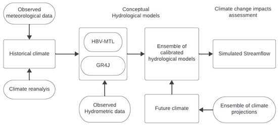
Figure 1.
Framework for climate change assessment on streamflow in LRB.
2.1. Historical Hydroclimatic Datasets
The CRB watershed polygon shapefiles and digital elevation models (DEMs) were utilized for the delineation of sub-watersheds and the mapping of the river network. The procedures involved using ESRI ArcGIS Desktop [71]. Land cover data were retrieved based on ENVISAT’s Medium Resolution Imaging Spectrometer (MERIS) Level 1B data, acquired in full-resolution mode with a spatial resolution of approximately 300 m [72]. OpenStreetMap (OSM) features under infrastructure, mining, and fabrication were obtained through the UN Humanitarian Data Exchange.
Streamflow observations from the hydrometric station at the watershed’s outlet were obtained from the International Commission for the Congo-Ubangi-Sangha Basin [17]. Precipitation and temperature gauge observations were obtained from the National Meteorological Agency of the Democratic Republic of Congo. Missing data patterns and mechanisms were analyzed during data preparation. Construct-level missingness in the dataset was the primary consideration when selecting the study period for the calibration and validation of hydrological models. Based on the demonstrated reliability over the African continent [73,74,75], two reanalysis products, ERA5 and MERRA-2, were considered for collecting temperature and precipitation data at acceptable spatial and temporal resolutions over the watershed, as shown in Table 1.

Table 1.
Climate reanalysis datasets.
2.2. Climate Model Projection
The NASA Earth Exchange Global Daily Downscaled Projections dataset featured 19 General Circulation Models’ (GCMs’) outputs (NEX-GDDP; available at https://cds.nccs.nasa.gov/nex-gddp/ accessed on 1 June 2024) that accounted for bias-corrected daily minimum and maximum near-surface air temperatures and precipitation, at a spatial resolution of 0.25°, based on the outcomes of CMIP6. Daily downscaled models were generated by adapting the monthly bias correction/spatial disaggregation (BCSD) approach [76]. Future climate projections were covered amongst three timeframes, including near-term (2021–2040), mid-term (2041–2070), and long-term (2071–2100), from SSP2-45 and SSP5-85 that respectively represent moderate and predominant mitigation challenges until the end of the century.
The SSP scenarios were developed to investigate global development trajectories with regard to climate change. They assess the impact of socioeconomic trends and policies on greenhouse gas emissions, climate change, and societal resilience [77]. SSP2-45 depicts global development progress steadily facing challenges in addressing climate change. Despite some advancements in reducing emissions, it may not be adequate to mitigate the effects of climate change by the end of the century [43]. SSP5-85 depicts a high-emission scenario characterized by reliance on fossil fuels and limited efforts to tackle climate change. This pathway anticipates an increase in greenhouse gas emissions resulting in climate impacts [45]. These pathways contribute to climate modelling by projecting how various policy decisions and societal shifts could influence conditions [78].
2.3. Hydrological Models
Simplicity and accuracy [77] were the principal criteria for selecting the HBV-MTL and GR4J models used in this study to simulate daily streamflow in the LRB. The HBV-MTL model shown in Figure 2 represents the hydrological processes using a set of equations and parameters.
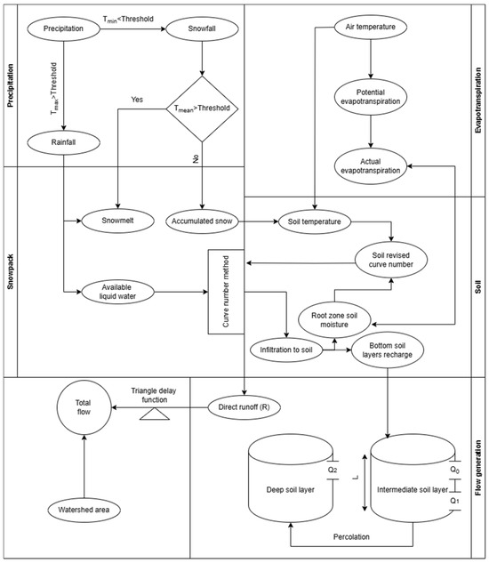
Figure 2.
A schematic of the HBV-MTL hydrological model.
Conceptual HBV models are widely used for streamflow estimations at watershed outlets [79,80]. A variant of the HBV model was introduced by [81] based on [82], namely HBV-MTL. This model employs daily temperature and precipitation data as its primary inputs. It differentiates precipitation into the categories of rainfall, snowfall, or a mix of both, according to a temperature threshold. Rainfall and any resulting liquid water from melted snow may infiltrate the soil layer, contributing to soil moisture or surface runoff. The amount of the contribution split depends on the current soil temperature and moisture conditions.
Evapotranspiration was calculated based on Hargreaves’ method [83]. This method is widely used and validated in various regions worldwide for its accuracy in estimating evapotranspiration. Numerous studies have compared the process with other models and observed reasonable results, making it a reliable tool for calculating evapotranspiration [84,85,86]. The method is based on the mean, maximum, and minimum air temperature and extraterrestrial radiation.
The remaining water percolates into deeper soil layers, contributing to the formation of interflow and baseflow and replenishing groundwater. Interflow is the lateral movement of water through the subsurface layers of soil, while baseflow refers to the slow and continuous movement of water into streams and rivers [87]. Total runoff is the sum of surface flow, interflow, and baseflow. It is assigned to a triangular delay function to simulate the daily streamflow at the watershed outlet. A balanced hydrological system regulates water availability, preventing both water scarcity and excessive flooding while maintaining the overall stability and resilience of ecosystems [88].
The GR4J model shown in Figure 3 is a numerical system that calculates runoff using daily data on precipitation, temperature, and potential evapotranspiration. Distinct from the HBV-MTL model, GR4J partitions the net precipitation, which is derived by deducting potential evapotranspiration from total precipitation, into two segments. This model comprises three primary components: production storage, routing storage, and dual unit hydrograph functions. Initially, a segment of net precipitation is allocated to production storage, where it percolates slowly based on soil moisture capacity. Concurrently, a portion of stored water facilitates evapotranspiration through vegetation usage. The remaining net precipitation merges with the water that percolated from the production storage and directed to the routing storage via unit hydrographs, which manage the delay between precipitation events and streamflow generation. At this juncture, 10% of the runoff is directly channelled to the outlet using a two-sided unit hydrograph. In contrast, the residual 90% is indirectly routed through interactions with groundwater, employing a one-sided unit hydrograph. Further information on the model’s architecture and equations is provided in [89].

Figure 3.
A schematic of the GR4J hydrological model.
The calibration process involves adjusting the parameters of the HBV-MTL and GR4J models to ensure they accurately simulate the historical hydrological processes. This is conducted by comparing the model outputs with the historical data and iteratively refining the parameter to a satisfactory threshold. Parameterizing hydrological models can be challenging. Selecting suitable values for model parameters is a key step for this endeavour because parameter values greatly influence the model’s behaviour and performance.
Both hydrological models were calibrated against observed streamflow data from gauges at the outlet. The primary input consisted of an ensemble of climate datasets from the historical period, including station-based observations, an ensemble of GCMs, and reanalysis datasets.
The Kling–Gupta efficiency (KGE) measure [90] was used to evaluate the models’ performance. It compared the estimated and observed values across many statistical criteria, enabling a thorough assessment of the hydrological models. KGE was used to assess the estimated values from the model using an array of statistical criteria and comparing them with the observed values. It comprehensively evaluated the hydrological models, considering several factors, including the correlation, variability, and bias between the observed and estimated values. This aids in assessing the accuracy and precision of simulations and forecasts of hydrological processes.
The criteria for formulating the KGE metric include standard deviation, mean, and Pearson correlation coefficient, represented as α, β, and μ, respectively, in the equations (1, 2, and 3). Compared to other measures such as Nash–Sutcliffe efficiency, KGE provides a more balanced assessment by incorporating these criteria via the Euclidean distance measure [91]. This approach enables a robust assessment of model accuracy and reliability. The calibration and evaluation of the hydrological models are conducted using KGE measures on both the daily and annual scales, as outlined in (5). The standard deviations of simulated and observed runoff are represented in Equations (1–3) as σS (simulated standard deviation) and σO (observed standard deviation). Meanwhile, S̅ and O̅ refer to the mean values of simulated and observed flow, respectively, and St and Ot represent specific instances of simulated and observed flow. Below are the equations used to calculate these values:
The Shuffled Complex Evolution algorithm (SCE-UA), developed by Duan et al. (1993) and further explored by Yarpiz (2020), was employed to calibrate the hydrological models. This is a method that integrates both random [92] and deterministic strategies [93], along with clustering [94] and competitive evolution [95], to optimize parameter sets. The optimization occurs through a global search mechanism that mimics natural evolutionary processes [96,97]. Initially, a population of parameter sets was randomly selected from the feasible space and subsequently divided into several complexes. These complexes evolved independently using a competitive evolution technique. The populations were periodically shuffled to prevent the algorithm from settling into local optima, enabling information interchange between complexes. This iterative procedure continued until the convergence criteria were met. In the specific context of this study, 50 parameter sets were randomly chosen within the defined range and segmented into five complexes. The evolution and shuffling of the complexes persisted through a maximum of 100 iterations to ensure a thorough exploration of the parameter space.
3. Case Study
The Congo River Basin (CRB), as shown in Figure 4, is located between latitudes 9° N and 14° S and longitudes 11° E and 34° E. Extending across Central Africa, the CRB is ranked after the Amazon River Basin as the second largest watershed in the world, with an impressive 3.7 million square kilometres and a mean annual discharge of 40,600 m3/s [98]. Surrounding most of the Democratic Republic of the Congo’s (DRC’s) territory, the CRB also extends its coverage to eight other countries. These countries include Angola, Burundi, the Central African Republic, Cameroon, the Republic of the Congo, Tanzania, Rwanda, and Zambia. The CRB supports the Congo rainforest, which is one of three major humid tropical regions on Earth [99].
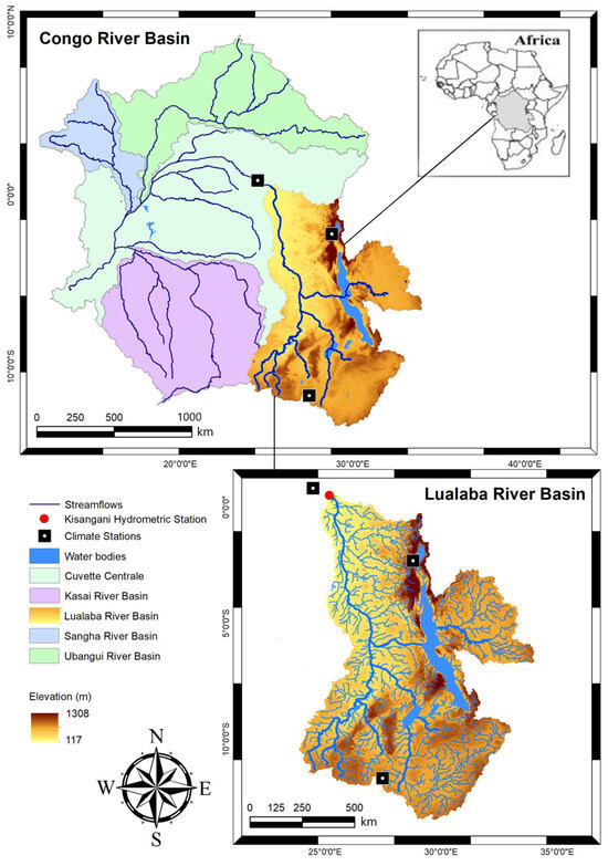
Figure 4.
CRB sub-watershed, Lualaba River Basin, location of gauges used in case study.
The Lualaba River Basin (LRB) is amongst the largest of five sub-watersheds, accounting for 27% of the total area of the CRB [23]. It drains approximately 974,140 square kilometres, most of which is located within the DRC. The remaining area coverage is located across Zambia in the southeast and Rwanda, Burundi, and Tanzania in the east. As a major contributor to the CRB’s annual water budget, the LRB is a principal agent for water resource management in the region [100]. However, this region is ranked 177 of 181 on the Notre Dame Global Adaptation Initiative (ND-GAIN) Country Index, illustrating countries that are best prepared to deal with global changes brought about by overcrowding, resource constraints, and climate disruption [101]. There is an unequal distribution of population in the LRB, accounting for over 30% of the DRC’s population, including several conflicted regions that are often portrayed as prominent examples of how violent struggles over natural resources have shaped internal warfare [102].
A plethora of critical mineral resources, including cobalt, coltan, copper, and other valuable minerals, exist in this region [103,104,105]. However, the predominant economic activity sustaining local households is shifting agriculture, which is profoundly reliant on the availability of water resources within the region. Notably, agricultural productivity within the LRB is predominantly rain-fed, rendering the basin’s water availability critical for ensuring regional food security [106]. In the Supplementary Materials, Figure S1 illustrates aspects of the LRB’s land use distribution, emphasizing its water resources and soil and vegetation cover. Water resources are depicted, showcasing the extensive network of rivers and streams within the watershed. Hydraulic infrastructure represents the locations of dams or other facilities essential for regulating the flow, hydropower, and distribution of water. Soil cover delineates the primary areas of fertile land, while civil and mining activities represent locations of interest where industrial and extractive operations are concentrated. Vegetation cover illustrates expansive areas of natural flora across the watershed. Furthermore, a UNESCO World Heritage Sites collection is located within the LRB. These National Parks, namely Kahuzi-Biega, Kundelungu, Maiko, Upemba, and Virunga, collectively cover 50,000 square kilometres as a habitat for numerous endangered species of animals and fish, thereby emphasizing the LRB’s ecological significance.
The Lualaba River is the principal headstream of the LRB, flowing entirely within the DRC’s national borders. It is a testament to the power and beauty of nature and an important asset in the ecosystem of the CRB. Spanning an impressive 1800 kilometres, the Lualaba River originates at approximately 1400 m above sea level on the Katanga (Shaba) Plateau near Musofi; the river’s early watercourse features a descent across the Manika Plateau, marked by numerous waterfalls and rapids. Notably, the river undergoes a drastic descent into the Upemba depression, dropping about 457 m over 72 kilometres, a gradient harnessed for hydroelectric production at the Nzilo Dam near the historical Delcommune Falls [107].
The river becomes navigable at Bukama, continuing for roughly 644 kilometres through the channel, where it expands into expansive, marsh-filled lakes like Upemba and Kisale, which are prone to seasonal flooding and dense with aquatic vegetation [108]. Along this navigable stretch, the Lualaba River is fed by tributaries such as the Lufira, Luvua, and Lukuga rivers. Downstream, the Lualaba River enters the challenging Portes d’Enfer (Gates of Hell), a narrow and deep gorge that precludes navigation. The river is again navigable for 109 kilometres from Kasongo to Kibombo, although this segment is interrupted by rapids extending to Kindu. Despite some shallow sections and rocky banks toward its outlet near Kisangani, the river remains navigable up to the Boyoma Falls, where a series of seven cascades marks the transition of the Lualaba River into the Congo River [109]. The historical hydroclimatic characteristics of the LRB are presented in Table 2.
Table 2.
The hydroclimatic characteristics of the LRB.
Daily streamflow and the flow duration curve recorded at the Kisangani hydrometric station are presented in Figure 5. The left panel presents the daily streamflow recorded at the outlet for each year from 1981 to 2001, revealing interannual streamflow variations and peak periods that indicate seasonal influences. The right panel presents daily streamflow against exceedance probabilities over the same time period, as the river’s perennial characteristic. Low streamflow was recorded around 5000 m3/s, medium flow at approximately 7500 m3/s, and high flow above 11,000 m3/s.
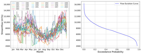
Figure 5.
LRB outlet, daily streamflow and flow duration curve (1981–2001).
Historical temperature and precipitation datasets revealed a mean annual temperature between 22 °C and 25 °C and mean annual precipitation varying from 1385 to 1526 mm over the LRB for a 20-year period (1981–2001). Temporal variations in the daily mean precipitation and temperature across the LRB, along with seasonal climatic cycles derived from reanalysis products and gauge observations from 1981 to 2001, are detailed in Figure 6 which employs boxplots to represent daily values averaged over gauge observations and lines to depict expected daily temperature and precipitation over the 20-year period. The boxplots clearly depict the central tendency and dispersion of the daily precipitation and temperature for each dataset. Notably, the range of values for the reanalysis datasets varies significantly, principally with regard to precipitation. Such discrepancies may stem from differences in assimilation schemes, the ground data incorporated into assimilation processes, and the forecasting climate models [110].

Figure 6.
(a,b) Daily precipitation and temperature (left panel). Observed daily (boxplots) and expected values (lines) per month based on observation and reanalyses (right panel).
Gauge observations revealed a median daily precipitation of approximately 1.8 mm, with an interquartile range (IQR) extending from approximately 0.3 mm to 5.8 mm. The maximum daily precipitation recorded was around 13.8 mm. The MERRA-2 dataset had a higher median of 3.2 mm but a slightly narrower distribution, indicating less variability. The IQR ranged from 1.3 mm to 5.6 mm, with a maximum value near 12 mm. ERA5 revealed the lowest median precipitation at around 1.8 mm, with a much narrower distribution. Its maximum daily precipitation was roughly 6 mm, and the IQR ranged between 0.8 mm and 3.1 mm. Temperature, on the other hand, ranged from 19 °C to 25 °C for the gauge observations, the IQR ranged from 21.4 °C to 22.9 °C, and it had a mean of 22 °C. MERRA-2’s mean daily temperature was 22.9 °C, IQR was from 22.2 °C to 23.8 °C, and it had a maximum and minimum of 26 °C and 19.6 °C, respectively. Similarly, a mean temperature of 23 °C was recorded by ERA5, however with a narrower IQR.
The right panels of Figure 6 highlight seasonal variations, presenting daily precipitation and temperature boxplots for each month. Observation unveiled two high precipitation periods during March-April-May (MAM) and September-October-November (SON), with peaks in April and November exceeding 12 mm/day. MERRA-2 unveiled a lower variability and magnitude in precipitation compared to observed data, with peaks in March, and ERA5 consistently recorded lower precipitation values and less variability throughout the year. For temperature, observation indicated a distinct seasonal cycle, with temperatures peaking in March and April (over 23 °C) and the coolest period from June to August (around 21 °C). MERRA-2 captured the seasonal cycle well, generally indicating slightly higher temperatures than gauge observations, while ERA5 followed the observed seasonal cycle but reported consistently higher temperatures.
The gauge observations unveiled the most variability in precipitation and higher peaks, essential for capturing extreme weather events. MERRA-2 aligned well with the precipitation cycle but overestimated variability, while ERA5 consistently showed lower values. The observed temperature data accurately reflected seasonal dynamics. MERRA-2 showed good alignment to the cycle with slight overestimation, while ERA5 consistently recorded higher temperatures. For the purpose of hydrological model calibration, the ERA5 and MERRA-2 reanalysis datasets provided reliable insight into precipitation and temperature over the LRB.
On the basis of the Phase 6 CMIP6 results, NEX-GDDP provided bias-corrected daily minimum and maximum near-surface air temperatures and precipitation. SSP2-45 and SSP5-85 represented moderate- and high-forcing scenarios until the year 2100 over the watershed (2021–2040, 2041–2070, and 2071–2100). A comparison of historical data (1981–2001) with future projections across various time horizons is provided in Figure 7 to illustrate the temporal variation in daily precipitation and temperature. Outputs from 19 GCMs were computed along with gauge observations and reanalysis products from ERA5 and MERRA-2 under two shared socioeconomic pathways (SSP2-4.5 and SSP5-8.5). The magnitudes of daily precipitation and temperature for the historical period are presented in the first panel. (a) The median precipitation recorded by GCMs was 4.1 mm, IQR ranged from 1.9 mm to 5.5 mm, and a maximum of 9.1 mm was recorded. (b) The mean daily temperature recorded by GCMs was 25.3 °C, IQR ranged from 25 °C to 25.7 °C, and maximum and minimum temperatures of 26.7 °C and 24.2 °C were recorded, respectively.
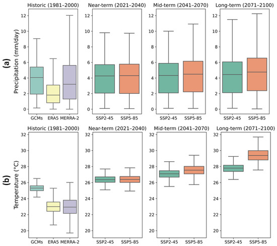
Figure 7.
Climate model projections under SSP2-45 and SSP5-85 compared with historical (a) precipitation and (b) temperature (GCMs and reanalysis in the LRB).
The right panels in Figure 7 represent precipitation and temperature projections for near-term, mid-term, and long-term periods under two scenarios: SSP2-45 and SSP5-85. (a) Both SSP2-45 and SSP5-85 projected a near-term median daily precipitation of 4.3 mm, IQR from 2 mm to 5.7 mm, and a maximum of 9.8 mm. Mid-term projections under SSP2-45 maintained a median daily precipitation of 4.3 mm, IQR from 2.1 mm to 5.9 mm, consistent precipitation range, and maximum at 10 mm. SSP5-85 continued to show similar patterns, with a median at 4.5 mm, slightly broader IQR of 2.3 to 6.2, and maximum of 11 mm. As for the long-term climate projections under SSP2-45, the median daily precipitation was 4.4 mm, IQR was from 2.1 mm to 6.1 mm, and maximum precipitation was 11.5 mm. SSP5-85 projected higher precipitation variability, a median at 4.7 mm, and a maximum reaching 12 mm. (b) The mean daily temperature projections under SSP2-45 were 26.4 °C for the near-term, with IQR ranging from 26 °C to 26.7 °C, and a maximum and minimum temperature of 27.7 °C and 25.1 °C, respectively.
Although there were slight increases in variability, a similar median was projected by SSP5-85 with maximum and minimum daily temperatures of 28 °C and 25 °C, respectively. The mid-term projections under SSP2-45 maintained a mean daily temperature of 27 °C, IQR from 26.7 °C to 27.5 °C, and a maximum and minimum temperature of 28.8 °C and 25.4 °C. Temperature patterns remained similar under SSP5-85, with a mean of 27.6 °C, IQR that was slightly broader, and a maximum and minimum temperature of 29.9 °C and 25.7. The mean daily temperature under SSP2-45 for the long term was 27.8 °C, and the IQR ranged from 27.4 °C to 28.2 °C. A considerable increase was noticed under SSP5-85 that projected a mean daily temperature of 29.4 °C, IQR from 28.8 °C to 30 °C, and maximum and minimum reaching 32 °C and 27.6 °C, respectively.
The historical data revealed differences in rainfall and temperature among various datasets. ERA5 was in closer alignment to MERRA-2, compared to historical GCM outputs. Looking into the future, both the SSP2-45 and SSP5-85 scenarios predicted stable rainfall for all future timeframes. However, the SSP5-85 scenario indicated higher variability. This implies that while average rainfall is likely to remain stable, there could be an increase in extreme rainfall events under higher-emission scenarios. Temperature forecasts unveiled an increasing trend over time. Short-term predictions hinted at a rise in temperature. Mid-term and long-term projections under SSP5-85 pointed to a significant increase, in both average temperatures and variability.
4. Results
4.1. Hydrological Model Performance during the Historical Period
The historical period from 1981 to 2001 was selected based on the availability of climate datasets and streamflow data within the LRB. The HBV-MTL and GR4J models were calibrated using temperatures and precipitation from two reanalysis datasets and the average historical outputs from 19 GCMs. The KGE statistical metric was used to assess the performance of the hydrological models. The calibration performances of the hydrological models are presented in Table 3 and validation performances in Table S1 under Supplementary Materials. Any optimal solutions that recorded KGE < 0.4 and KGE < 1.5 for the calibration of HBV-MTL and GR4J, respectively, were considered unsatisfactory and were attributed to low-quality model input data from gauge observations, including streamflow. Models that did not converge to an optimal solution and those that did not meet the calibration thresholds were not considered for the assessment under projected future climate.
Table 3.
Calibration performance of HBV-MTL and GR4J models.
HBV-MTL models revealed acceptable performance across reanalysis-based configurations, especially under the historical GCM configuration. On the other hand, GR4J models systematically returned lower performance in comparison to HBV-MTL models, with the exception of the ERA5-based configuration. Performance assessment indicated that MERRA-2 was the least efficient dataset for the calibration of hydrological models. The GR4J model showed good model performance under the ERA5 configuration (KGE = 0.49), whereas HBV-MTL performed well under the GCM configuration (KGE = 0.59). In contrast, the ERA5 and MERRA-2 configurations returned negative NSE values, suggesting that they might be less reliable than using the average of the input data as predictors. Across all configurations, there was a positive linear relationship. In addition, the relative bias revealed the tendencies of models to overestimate or underestimate the streamflow for each configuration.
Daily and annual streamflow at the LRB outlet for gauge observation and simulations with HBV-MTL and GR4J are presented in Figure 8 (HBV-MTL on the left panel and GR4J on the right panel). Each time series presents the observed and simulated daily streamflow (solid lines), as well as observed and simulated annual streamflow (dashed lines).
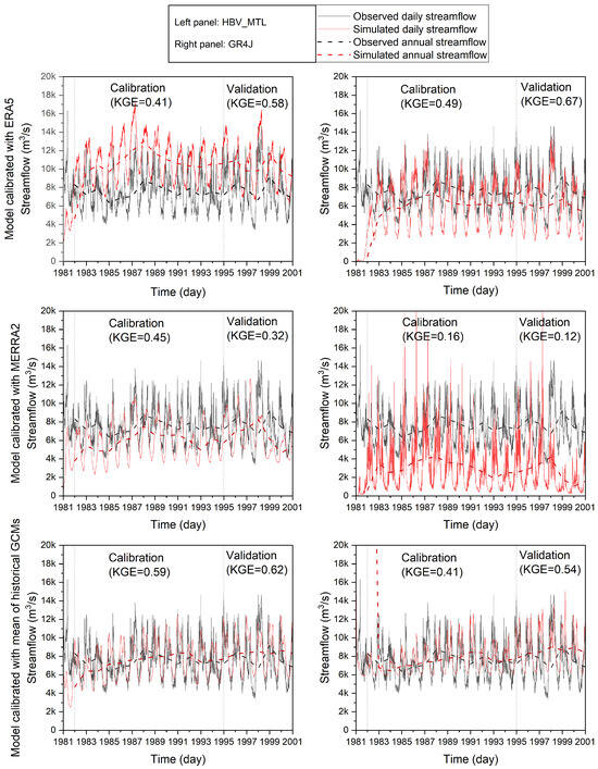
Figure 8.
Observation and simulation of daily and annual streamflow for historical period at Kisangani.
The calibration and validation periods are clearly outlined in Figure 8, with Kling–Gupta efficiency (KGE) values providing a quantitative measure of model performance. Distinct patterns emerged in the performance of the HBV-MTL and GR4J models during the calibration and validation stages. When utilizing ERA5 reanalysis data for calibration, the HBV-MTL model tends to overestimate observed streamflow. Conversely, under the ERA5 configuration, the GR4J model generally underestimates observed streamflow. With MERRA-2 configuration, both the HBV-MTL and GR4J models tend to underestimate the observed streamflow. This consistent underestimation hints at biases in MERRA-2 data or shortcomings in representing certain hydrological processes within these models using this dataset. When the hydrological models were calibrated with historical GCMs, they exhibited an alignment with the observed streamflow. This alignment suggests that the models can effectively reproduce the patterns when historical GCM data are utilized, highlighting the potential of these models to serve as tools for simulating streamflow under past climate conditions. In general, the results of calibration and validation emphasize the varying performance of the HBV-MTL and GR4J models based on the input data.
The long-term historical annual runoff shown in Figure 9 presents observed flow (solid black line), optimal flow for calibration (solid green line), observed flow for validation (solid blue line), and optimal flow for validation (solid red line). Across configurations, both hydrological models captured fluctuations in streamflow, including high- and low-flow periods, as well as the seasonality. Generally, the ERA5 configuration aligned well with gauge observations for both hydrological models, particularly during the calibration period. Notably, this alignment reflects high-flow periods from March to May and September to November and low-flows period from June to August. Discrepancies were more pronounced in the MERRA-2-based models, especially concerning the HBV-MTL model during low-flow months from June to August. The historical GCM-based models showed good performance by representing seasonal changes and closely matching the observed and simulated streamflow. The findings underscore the significance of choosing input data for modelling. The ERA5 configurations seemed effective for both the HBV-MTL and GR4J models, whereas adjustments may be required for the MERRA-2 configurations to better capture low-flow periods. The historical GCM-based models present a viable option for capturing long-term seasonal variations in streamflow.
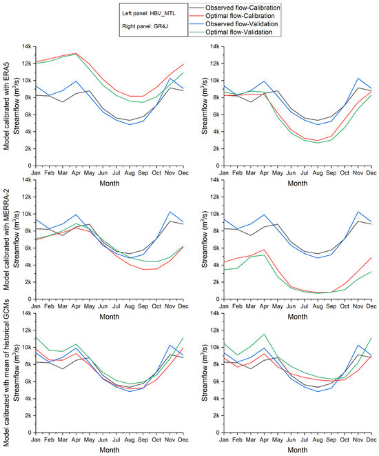
Figure 9.
Long-term annual hydrograph observation and simulation at outlet using reanalysis datasets with HBV-MTL (left) and GR4J (right) models.
4.2. Streamflow Conditions under GCM Projections of Changing Climate
To estimate streamflow at the LRB outlet for future horizons, 19 GCMs under SSP2-45 and SSP5-85 were respectively forced into the hydrological models according to the scenarios. The observed and projected interannual hydrographs using HBV-MTL as presented in Figure 10 revealed changes in peak timing and seasonality, as well as an overall increase in the magnitude of runoff across all model configurations. The increase is more pronounced under the SSP5-85 scenario.
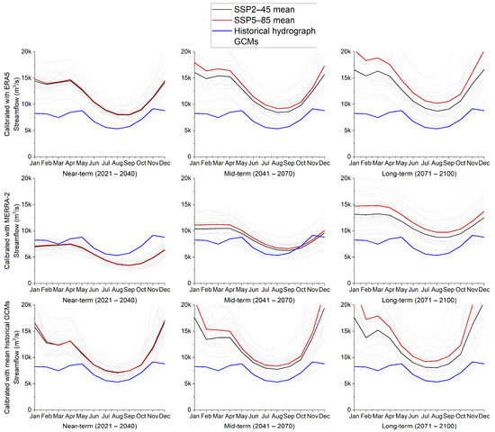
Figure 10.
Mean annual hydrograph at LRB outlet under SSP2-45 and SSP5-85 using HBV-MTL model calibrated with ERA5, MERRA-2, and GCMs.
ERA5-based models revealed a general increase in annual discharge under SSP2-45 and SSP5-85 compared to the long-term historical hydrograph across all future horizons. GCM-based models also displayed an increase in discharge across future time periods. MERRA-2-based models showed a decline in discharge compared to the long-term historical hydrograph for the near future, followed by an increase in the mid- to long-term future.
The observed and projected interannual hydrographs with GR4J models are presented in Figure S2 of Supplementary Materials. Similar to the projections with HBV-MTL, the hydrographs revealed changes in peak timing and seasonality. However, these patterns differ in high and low flows, which are accentuated in this case. Overall, the annual hydrographs indicated an increase in discharge across future horizons for the ERA5 and GCM configurations, with a more pronounced increase under SSP5-85. MERRA-2 configurations, however, revealed a decrease in discharge compared to the long-term historical hydrographs across all future horizons, where the difference between SSP2-45 and SSP5-85 remained more pronounced in the long term, especially for periods for high flow.
A better understanding of the runoff conditions in the future is provided by analyzing the changes in the 90th, 50th, and 10th flow percentiles. Thus, observed and simulated annual flow duration curves (i.e., empirical cumulative probability distributions of runoff in each year) were analyzed for historical and future periods. Figure 11 and Figure S3 in the Supplementary Materials illustrate the variability in projected changes in streamflow quantiles under the SSP scenarios and future time periods, for the HBV-MTL and GR4J models, respectively.
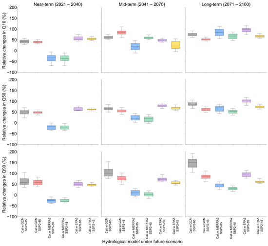
Figure 11.
Relative changes between simulated annual streamflow quantiles under SSP2-45 and SSP5-85 according to outputs of 19 GCM projections using HBV-MTL.
Streamflow values were averaged over the historical period to calculate the long-term historical interannual quantiles. Similarly, based on the outputs of the SSP2-45 and SSP5-85 scenarios, with an ensemble of 19 GCMs, the long-term projected interannual quantiles were calculated for six hydrological model configurations.
The magnitude and direction of relative change in annual flow quantiles varies depending on model configuration and considered future horizon. An overall increase in interannual quantiles for low, median, and high flows was found across all projected time horizons for the HBV-MTL and GR4J models, with the exception of GR4J-MERRA-2 and GR4J-ERA5. In comparison to historical annual flow quantiles, the HBV-MTL models configured with MERRA-2, as shown in Figure 11, projected a nuanced trend. Specifically, there was an initial decline in Q10, Q50, and Q90 during the near term (2021–2040). This decline was followed by a slight increase during the mid-term (2041–2070), which then transitioned into a more significant rise in the long term (2071–2100). These projections indicate that while the near term may experience reduced streamflow, the latter half of the century could see substantial increases in low, median, and high flows. Conversely, under the ERA5 and GCM configurations, the HBV-MTL models revealed a consistent increase in annual flow quantiles Q10, Q50, and Q90 across all future periods.
For the GR4J models configured with ERA5, as depicted in Figure S3, there was a clear pattern where the low flow (Q10) was projected to decrease across all future horizons. In contrast, both the mid flow (Q50) and high flow (Q90) were projected to increase. This potential shift in variability could imply more pronounced extreme runoff events. GR4J models that were configured with MERRA-2 projected a decrease in annual flow quantiles Q10, Q50, and Q90 throughout future horizons. Models configured with historical GCMs, however, projected a considerable increase in Q10, Q50, and Q9. The increase was observed particularly during the near term (2021–2040).
The Mann–Kendall trend test is a nonparametric method often used in climate change impacts assessments [111,112]. This method was applied to analyze trends in annual flow quantiles and determine their significance for future projections. The summary test results of expected future annual Q10, Q50, and Q90 values for all model configurations are presented in Table S2 of the Supplementary Materials. The Mann–Kendall trend analysis revealed an increasing trend across all model configurations under both SSP2-45 and SSP5-85. Figure 12 highlights trends in projected future high flows (Q90) under SSP scenarios with respect to specific model configurations. The analysis revealed a significant increasing trend in high flow across all models for both the SSP2-45 and SSP5-85 scenarios. Notably, the increasing trend was more pronounced under the SSP5-85 scenario compared to SSP2-45. Similar trends were observed for projected low flow (Q10) and median flow (Q50), as shown in Figures S4 and S5 of the Supplementary Materials, respectively. Similarly, Figures S4 and S5 in the Supplementary Materials illustrate trends in projected low flow (Q10) and median flow (Q50), respectively. Overall, the results from the Mann–Kendall trend analysis provide strong evidence of significant increases across annual flow quantiles under future climate scenarios.
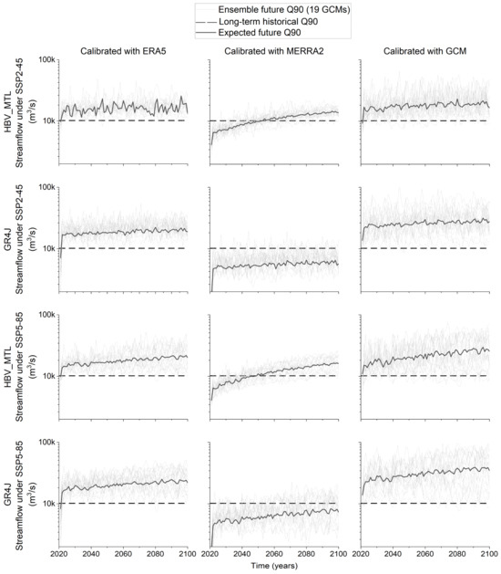
Figure 12.
Ensemble and expected future values of annual Q90 under SSP2-45 and SSP5-85 based on calibrated HBV-MTL and GR4J models using ERA5, MERRA-2, and GCM reanalyses.
5. Discussions
This study assessed the possible impacts of climate change on streamflow characteristics using a multi-model framework over the LRB, an important watershed in the Congo River Basin, Central Africa. For this purpose, two conceptual hydrological models, HBV-MTL and GR4J, were calibrated using two reanalysis products, as well as an ensemble of historical GCMs. Subsequent to the calibration, the hydrological models were fed with downscaled bias-corrected outputs from 19 GCMs under two shared socioeconomic pathways, SSP2-45 and SSP5-85.
The results demonstrate that both hydrological models can simulate the observed runoff in the LRB with acceptable performance. The thresholds considered were demystified in several studies across the overarching CRB [16,113]. The KGE values indicated that all six configurations of hydrological models based on reanalysis and historical GCMs performed better than their counterparts that used gauge observations as input data. Such results align with other research in demonstrating that the superior performance of hydrological models configured with reanalysis products underscores the importance of incorporating an approach with an ensemble of data into hydrological modelling to improve performance [60,114,115]. The calibration results during the historical period (1981–2001) indicate that the performance of hydrological models is sensitive to the choice of reanalysis dataset and hydrological model structure. The results are consistent with related research [16,113,116,117] that highlights the importance of using high-quality input data along with a suitable model structure to achieve satisfactory calibration. Considering annual and daily time series, models that were configured with the historical ensemble of GCMs performed better than the others.
Streamflow projections under the SSP2-45 and SSP5-85 scenarios provide valuable information on the hydrological response to climate change in the LRB. Overall, the projected simulations under climate change scenarios indicate that runoff is expected to increase with a change in peak timing and seasonality. However, the expected change in the magnitude of future annual hydrographs depends on the considered hydrological model configuration. The projected runoff increase is more pronounced under the SSP5-85 scenario. Based on a comparison between observed and future values, changes in the mean annual discharge at the outlet of the LRB are estimated to range from 45% to 62%. Considering the shift in peak timing and seasonality, across model configurations, the results suggest a shorter high-flow cycle, revealed by an earlier peak during March-April-May (MAM) and late peak during September-October-November (SON). These results imply the likelihood of extreme runoff event occurrence in the future. Other studies within the CRB concurred with these findings [16,118,119,120,121]. According to Aloysius and Saiers (2017), decreases in rainfall in the southern headwater areas of the CRB have resulted in prolonged periods of low flow in comparison to the reference period of 1986–2005, and a 10.4% runoff increase was observed over the southwest region under high-emission scenarios from 2046 to 2065.
Projected changes in annual flow quantiles (Q10, Q50, Q90) further elucidate the hydrological conditions in response to climate change in the LRB. While an overall increase in annual quantiles was observed based on all model configurations, the magnitude and sign varied among each configuration. The analysis revealed that Q10 is projected to increase by 33% and 44% under SSP2-45 and SSP5-85, respectively. These projections suggest a significant rise in low-flow conditions, potentially reducing the frequency of extreme low-flow events and improving water availability during dry periods. Similarly, Q50 is projected to increase by 32% under SSP2-45 and 44% under SSP5-85. The rise in Q50 implies an uptick in median streamflow, pointing to improved water availability, which could be advantageous for both human needs and the environment. Lastly, Q90 is projected to increase by 56% and 80% under SSP2-45 and SSP5-85, respectively. The considerable increase in Q90 indicates the likelihood of more frequent high-flow occurrences, which raises the threat of flooding. This projection underscores the need for flood control measures and strategies to safeguard both communities and infrastructure in the LRB.
The projected streamflow is presented in Figure 13. In the SSP2-45 scenario, the uncertainty range is relatively consistent, with periodic fluctuations in streamflow magnitude. The streamflow values generally remain within a lower range compared to SSP5-85, suggesting less variability in flow extremes. In contrast, the SSP5-85 scenario shows a broader and more variable range of streamflow values, especially in the latter part of the century. This reflects increased uncertainty and variability under a high-emission scenario, with more pronounced peaks in streamflow. The higher peaks and wider uncertainty bands suggest a greater likelihood of extreme flow events.
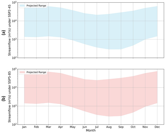
Figure 13.
Projected interannual streamflow under (a) SSP2-45 and (b) SSP5-85 climate scenarios.
The magnitude of streamflow in both scenarios tends to increase over time, particularly under SSP5-85. This trend indicates a growing potential for high-flow events. In SSP5-85, the maximum streamflow values occasionally exceed 200,000 m3/s, whereas SSP2-45 projections remain below this threshold. Moreover, the SSP5-85 scenario exhibits a higher degree of variability, evident from the larger vertical range in the uncertainty band, indicating greater fluctuations in projected streamflow. Such variability suggests that under a high-emission scenario, the LRB could experience more frequent and intense hydrological extremes.
Both scenarios exhibit a typical seasonal pattern with peak flows during the wet season and lower flows during the dry season. However, the SSP5-85 scenario shows a much steeper increase in streamflow towards the end of the year, suggesting more intense and potentially disruptive wet season events. In SSP2-45, the seasonal patterns are more consistent, with a relatively stable range of flow values, suggesting that moderate-emission pathways could help stabilize seasonal hydrological patterns.
Overall, the expected increase in flow underscores the importance of adaptive water management strategies. Such strategies should account for water storage capacity to guarantee a supply in times of low flow and effective flood protection measures to mitigate the impact of extreme flow events. The wider uncertainty range and higher maximum values in SSP5-85 highlight the need for robust flood management strategies. Additionally, the increased variability under SSP5-85 could complicate water resource planning, necessitating adaptive management strategies that can accommodate greater unpredictability in water availability. Considering the environment, these projections may or may not be beneficial for the ecosystem and its habitats, highlighting the need for ecosystem-based management strategies that cater to species and habitats. Ultimately, the different hydrological responses under climate scenarios and models underscore the significance of the multi-model approach to guide water management decisions.
6. Conclusions
This study builds upon an existing multi-model assessment of climate change impact in the Congo River Basin. It highlights the importance of hydrological models’ structure and input data used to forecast streamflow in historical contexts and future climate projections. The sensitivity of model outputs to both model structure and input data was considered in assessing the reliability of hydrological models, GCMs, and emission scenarios. The LRB presents unique challenges due to its data-scarce nature and complex hydrological processes. The use of multiple hydrological models and GCMs under different emission scenarios offers a comprehensive framework to evaluate climate impacts on streamflow. However, the large uncertainty observed across these projections indicates that no single model or scenario can be deemed universally reliable without considering context-specific factors.
The hydrological models used in this study were calibrated using both reanalysis products and historical GCM outputs. The results indicate that the choice of hydrological model significantly influences the simulation of streamflow, as each model has distinct structural characteristics that impact how it processes input data. For instance, HBV-MTL, with its more detailed representation of physical processes, may perform better in regions with substantial seasonal variability in precipitation and temperature. Conversely, GR4J’s simpler structure may be advantageous in regions where data limitations constrain the use of more complex models. This study found that models configured with reanalysis products generally performed better than those using meteorological gauge observations, highlighting the importance of high-quality, spatially comprehensive input data.
Precipitation, as the primary driver of streamflow, is particularly influential in determining the accuracy of hydrological model outputs. This study shows that the results are very sensitive to the choice of precipitation data, with discrepancies between different reanalysis products and GCMs contributing significantly to overall uncertainty. This sensitivity underscores the need for reliable precipitation data, which is lacking in the LRB. Bias-corrected and downscaled GCM outputs, such as those used in this study, help mitigate some of these issues but cannot completely eliminate uncertainty. The inherent variability in precipitation projections from different GCMs further complicates the interpretation of future streamflow scenarios, making it difficult to identify a single GCM or hydrological model configuration as the most reliable.
The two emission scenarios considered, SSP2-45 and SSP5-85, represent moderate- and high-radiative forcing pathways, respectively. The SSP2-45 scenario, which assumes more stringent climate policies, projects a relatively stable range of streamflow with less pronounced extremes. This suggests that moderate-emission pathways may help reduce the severity of hydrological impacts in the LRB. In contrast, the SSP5-85 scenario, which reflects high emissions and limited mitigation efforts, projects more significant variability and higher maximum streamflow.
The large uncertainty across all projections reflects the complex interplay between model structure, input data, and emission scenarios. This uncertainty is not only a result of differences in model configurations but also of the variability inherent in climate projections themselves. This study emphasizes that a multi-model approach is necessary to capture the range of possible hydrological responses and guide adaptive water management strategies. It is not enough to rely on a single model or scenario; rather, an ensemble of models and scenarios should be used to explore the full spectrum of potential outcomes.
Future research may broaden this investigation by including additional reanalysis products and hydrological models, as well as investigating a better representation of catchments (both lumped and semi-distributed models). Incorporating high-resolution regional climate models (RCMs) to capture local-scale climatic variations could improve the performance of hydrological models and help identify localized impacts of climate change on streamflow. Long-term, high-quality observational data in addition to integrating advance techniques such as machine learning and data assimilation can be used to enhance hydrological model performance and predictive accuracy. Investigations of the sensitivity of hydrological models to different climate data inputs, parameterization, and assumptions could help identify critical factors that influence model outcomes and guide efforts to reduce uncertainties. An exploration of the impacts of climate change on hydrological extremes is suggested, such as detailed studies on the frequency, intensity, and duration of floods and droughts. Better insights could be gained into the challenges facing future water resources by incorporating field data and taking into account socioeconomic aspects such as population growth and increasing water needs into a holistic approach.
Given the transboundary nature of the LRB, future research should explore collaborative water management approaches, including the development of frameworks for data sharing, joint modelling efforts, and coordinated adaptation strategies. Furthermore, future research should also investigate the potential geopolitical and social implications of hydrological changes, such as water allocation conflicts and the impacts on livelihood and food security. High-quality, long-term databases are essential for validating hydrological models and detecting hydrological patterns over time; therefore, it is a necessity to establish and maintain monitoring programs for the collection of continuous data on streamflow, precipitation, temperature, and other relevant variables.
By focusing on high-resolution climate models, improved hydrological modelling, integrated scenarios, extreme event analysis, ecosystem impacts, transboundary water management, and long-term monitoring, future research can provide critical insights and tools to support sustainable water resource management and climate adaptation in the region. These efforts will help ensure the resilience of the LRB’s water systems and the communities that depend on them.
Supplementary Materials
The following supporting information can be downloaded at https://www.mdpi.com/article/10.3390/w16192825/s1, Table S1: Validation performance of HBV-MTL and GR4J models; Table S2: Mann–Kendall summary trend analysis results for annual Q10, Q50, and Q90 based on ERA5, MERRA-2, and GCMs under SSP2-45 and SSP5-85; Figure S1: LRB land use classification; Figure S2: Mean annual hydrograph at LRB outlet under SSP2-45 and SSP5-85 using GR4J model calibrated with ERA5, MERRA-2, and GCMs; Figure S3: Relative changes between simulated annual streamflow quantiles under SSP2-45 and SSP5-85 according to outputs of 19 GCM projections using GR4J; Figure S4: Ensemble and expected future values of annual Q10 under SSP2-45 and SSP5-85 based on calibrated HBV-MTL and GR4J models using ERA5, MERRA-2, and GCM reanalyses; Figure S5: Ensemble and expected future values of annual Q50 under SSP2-45 and SSP5-85 based on calibrated HBV-MTL and GR4J models using ERA5, MERRA-2, and GCM reanalyses.
Author Contributions
Conceptualization, M.F. and E.H.; methodology, S.M. and E.H.; formal analysis, S.M.; data curation, S.M.; writing—original draft preparation, S.M.; writing—review and editing, S.M., M.F. and E.H.; visualization, S.M.; supervision, M.F. and E.H.; project administration, M.F. All authors have read and agreed to the published version of the manuscript.
Funding
This research was partly funded by NSERC (RGPIN-06979-2020), held by the second author.
Data Availability Statement
The original contributions presented in this study are included in the article; further inquiries can be directed to the corresponding authors.
Conflicts of Interest
The authors declare no conflicts of interest.
References
- Seiller, G.; Roy, R.; Anctil, F. Influence of three common calibration metrics on the diagnosis of climate change impacts on water resources. J. Hydrol. 2017, 547, 280–295. [Google Scholar] [CrossRef]
- Duan, K.; Caldwell, P.V.; Sun, G.; McNulty, S.G.; Zhang, Y.; Shuster, E.; Liu, B.; Bolstad, P.V. Understanding the role of regional water connectivity in mitigating climate change impacts on surface water supply stress in the United States. J. Hydrol. 2019, 570, 80–95. [Google Scholar] [CrossRef]
- Amanambu, A.C.; Obarein, O.A.; Mossa, J.; Li, L.; Ayeni, S.S.; Balogun, O.; Oyebamiji, A.; Ochege, F.U. Groundwater system and climate change: Present status and future considerations. J. Hydrol. 2020, 589, 125163. [Google Scholar] [CrossRef]
- Heidari, H.; Warziniack, T.; Brown, T.C.; Arabi, M. Impacts of Climate Change on Hydroclimatic Conditions of U.S. National Forests and Grasslands. Forests 2021, 12, 139. [Google Scholar] [CrossRef]
- Arnell, N.W. Climate change and global water resources. Glob. Environ. Change 1999, 9, S31–S49. [Google Scholar] [CrossRef]
- Wi, S. Impact of Climate Change on Hydroclimatic Variables. Ph.D. Thesis, The University of Arizona, Tucson, AZ, USA, 2012. [Google Scholar]
- Oguntunde, P.G.; Abiodun, B.J.; Lischeid, G. Impacts of climate change on hydro-meteorological drought over the Volta Basin, West Africa. Glob. Planet. Change 2017, 155, 121–132. [Google Scholar] [CrossRef]
- Alehu, B.A.; Desta, H.B.; Daba, B.I. Assessment of climate change impact on hydro-climatic variables and its trends over Gidabo Watershed. Model. Earth Syst. Environ. 2022, 8, 3769–3791. [Google Scholar] [CrossRef]
- Ganguli, P.; Coulibaly, P. Does nonstationarity in rainfall require nonstationary intensity–duration–frequency curves? Hydrol. Earth Syst. Sci. 2017, 21, 6461–6483. [Google Scholar] [CrossRef]
- Bourdeau-Goulet, S.-C.; Hassanzadeh, E. Comparisons Between CMIP5 and CMIP6 Models: Simulations of Climate Indices Influencing Food Security, Infrastructure Resilience, and Human Health in Canada. Earth’s Future 2021, 9, e2021EF001995. [Google Scholar] [CrossRef]
- Beven, K.; Westerberg, I. On red herrings and real herrings: Disinformation and information in hydrological inference. Hydrol. Process. 2011, 25, 1676–1680. [Google Scholar] [CrossRef]
- Nazemi, A.; Zaerpour, M.; Hassanzadeh, E. Uncertainty in Bottom-Up Vulnerability Assessments of Water Supply Systems due to Regional Streamflow Generation under Changing Conditions. J. Water Resour. Plan. Manag. 2020, 146, 04019071. [Google Scholar] [CrossRef]
- Zaerpour, M.; Hatami, S.; Sadri, J.; Nazemi, A. A novel algorithmic framework for identifying changing streamflow regimes: Application to Canadian natural streams (1966–2010). Hydrol. Earth Syst. Sci. Discuss. 2020, 2020, 1–39. [Google Scholar]
- Banda, V.D.; Dzwairo, R.B.; Singh, S.K.; Kanyerere, T. Hydrological modelling and climate adaptation under changing climate: A review with a focus in Sub-Saharan Africa. Water 2022, 14, 4031. [Google Scholar] [CrossRef]
- Majone, B.; Avesani, D.; Zulian, P.; Fiori, A.; Bellin, A. Analysis of high streamflow extremes in climate change studies: How do we calibrate hydrological models? Hydrol. Earth Syst. Sci. 2022, 26, 3863–3883. [Google Scholar] [CrossRef]
- Aloysius, N.; Saiers, J. Simulated hydrologic response to projected changes in precipitation and temperature in the Congo River basin. Hydrol. Earth Syst. Sci. 2017, 21, 4115–4130. [Google Scholar] [CrossRef]
- Laraque, A.; Nkaya, G.D.M.; Orange, D.; Tshimanga, R.; Tshitenge, J.M.; Mahe, G.; Nguimalet, C.R.; Trigg, M.A.; Yepez, S.; Gulemvuga, G. Recent budget of hydroclimatology and hydrosedimentology of the congo river in central Africa. Water 2020, 12, 2613. [Google Scholar] [CrossRef]
- Runge, J. The Congo River, Central Africa. In Large Rivers: Geomorphology and Management, 2nd ed.; John Wiley & Sons: Hoboken, NJ, USA, 2022; pp. 433–456. [Google Scholar]
- Brown, H.C.P.; Smit, B.; Sonwa, D.J.; Somorin, O.A.; Nkem, J. Institutional perceptions of opportunities and challenges of REDD+ in the Congo Basin. J. Environ. Dev. 2011, 20, 381–404. [Google Scholar] [CrossRef]
- Tshimanga, R.M.; Lutonadio, G.-S.K.; Kabujenda, N.K.; Sondi, C.M.; Mihaha, E.-T.N.; Ngandu, J.-F.K.; Nkaba, L.N.; Sankiana, G.M.; Beya, J.T.; Kombayi, A.M.; et al. An Integrated Information System of Climate-Water-Migrations-Conflicts Nexus in the Congo Basin. Sustainability 2021, 13, 9323. [Google Scholar] [CrossRef]
- United Nations Environment Programme. Water Issues in the Democratic Republic of Congo: Challenges and Opportunities—Technical Report; United Nations Environment Programme: Nairobi, Kenya, 2011. [Google Scholar]
- Diem, J.E.; Ryan, S.J.; Hartter, J.; Palace, M.W. Satellite-based rainfall data reveal a recent drying trend in central equatorial Africa. Clim. Change 2014, 126, 263–272. [Google Scholar] [CrossRef]
- Moukandi N’kaya, G.D.; Laraque, A.; Paturel, J.-E.; Gulemvuga, G.; Mahé, G.; Tshimanga, R.M. A new look at hydrology in the Congo Basin, based on the study of multi-decadal chronicles. ESS Open Arch. Eprints 2020, 105, 121–143. [Google Scholar] [CrossRef]
- Nicholson, S.; Klotter, D.; Zhou, L.; Hua, W. Validation of satellite precipitation estimates over the Congo Basin. J. Hydrometeorol. 2019, 20, 631–656. [Google Scholar] [CrossRef]
- Sidibe, M.; Dieppois, B.; Eden, J.; Mahé, G.; Paturel, J.-E.; Amoussou, E.; Anifowose, B.; Van De Wiel, M.; Lawler, D. Near-term impacts of climate variability and change on hydrological systems in West and Central Africa. Clim. Dyn. 2020, 54, 2041–2070. [Google Scholar] [CrossRef]
- Bhave, A.G.; Mishra, A.; Raghuwanshi, N.S. A combined bottom-up and top-down approach for assessment of climate change adaptation options. J. Hydrol. 2014, 518, 150–161. [Google Scholar] [CrossRef]
- Wilby, R.L.; Dessai, S. Robust adaptation to climate change. Weather 2010, 65, 180–185. [Google Scholar] [CrossRef]
- Gizaw, M.S.; Biftu, G.F.; Gan, T.Y.; Moges, S.A.; Koivusalo, H. Potential impact of climate change on streamflow of major Ethiopian rivers. Clim. Change 2017, 143, 371–383. [Google Scholar] [CrossRef]
- Krysanova, V.; Vetter, T.; Eisner, S.; Huang, S.; Pechlivanidis, I.; Strauch, M.; Gelfan, A.; Kumar, R.; Aich, V.; Arheimer, B. Intercomparison of regional-scale hydrological models and climate change impacts projected for 12 large river basins worldwide—A synthesis. Environ. Res. Lett. 2017, 12, 105002. [Google Scholar] [CrossRef]
- Sørland, S.L.; Schär, C.; Lüthi, D.; Kjellström, E. Bias patterns and climate change signals in GCM-RCM model chains. Environ. Res. Lett. 2018, 13, 074017. [Google Scholar] [CrossRef]
- Liang, X.Z.; Kunkel, K.E.; Meehl, G.A.; Jones, R.G.; Wang, J.X. Regional climate models downscaling analysis of general circulation models present climate biases propagation into future change projections. Geophys. Res. Lett. 2008, 35, L08709. [Google Scholar] [CrossRef]
- Diallo, I.; Sylla, M.; Giorgi, F.; Gaye, A.; Camara, M. Multimodel GCM-RCM ensemble-based projections of temperature and precipitation over West Africa for the early 21st century. Int. J. Geophys. 2012, 2012, 972896. [Google Scholar] [CrossRef]
- Okkan, U.; Kirdemir, U. Downscaling of monthly precipitation using CMIP5 climate models operated under RCPs. Meteorol. Appl. 2016, 23, 514–528. [Google Scholar] [CrossRef]
- Chen, J.; Brissette, F.P.; Chen, H. Using reanalysis-driven regional climate model outputs for hydrology modelling. Hydrol. Process. 2018, 32, 3019–3031. [Google Scholar] [CrossRef]
- Sharifinejad, A.; Hassanzadeh, E. Evaluating Climate Change Effects on a Snow-Dominant Watershed: A Multi-Model Hydrological Investigation. Water 2023, 15, 3281. [Google Scholar] [CrossRef]
- Ali, Z.; Iqbal, M.; Khan, I.U.; Masood, M.U.; Umer, M.; Lodhi, M.U.K.; Tariq, M.A.U.R. Hydrological response under CMIP6 climate projection in Astore River Basin, Pakistan. J. Mt. Sci. 2023, 20, 2263–2281. [Google Scholar] [CrossRef]
- Lauri, H.; de Moel, H.; Ward, P.J.; Räsänen, T.A.; Keskinen, M.; Kummu, M. Future changes in Mekong River hydrology: Impact of climate change and reservoir operation on discharge. Hydrol. Earth Syst. Sci. 2012, 16, 4603–4619. [Google Scholar] [CrossRef]
- Anaraki, M.V.; Kadkhodazadeh, M.; Morshed-Bozorgdel, A.; Farzin, S. Predicting rainfall response to climate change and uncertainty analysis: Introducing a novel downscaling CMIP6 models technique based on the stacking ensemble machine learning. J. Water Clim. Change 2023, 14, 3671–3691. [Google Scholar] [CrossRef]
- Eyring, V.; Bony, S.; Meehl, G.A.; Senior, C.A.; Stevens, B.; Stouffer, R.J.; Taylor, K.E. Overview of the Coupled Model Intercomparison Project Phase 6 (CMIP6) experimental design and organization. Geosci. Model Dev. 2016, 9, 1937–1958. [Google Scholar] [CrossRef]
- Masson-Delmotte, V.; Zhai, P.; Pirani, S.; Connors, C.; Péan, S.; Berger, N.; Caud, Y.; Chen, L.; Goldfarb, M.; Scheel Monteiro, P.M. IPCC, 2021: Summary for policymakers. In Climate Change 2021: The Physical Science Basis—Contribution of Working Group I to the Sixth Assessment Report of the Intergovernmental Panel on Climate Change; IPCC—Intergovernmental Panel on Climate Change: Geneva, Switzerland, 2021. [Google Scholar]
- Meehl, G.A.; Senior, C.A.; Eyring, V.; Flato, G.; Lamarque, J.-F.; Stouffer, R.J.; Taylor, K.E.; Schlund, M. Context for interpreting equilibrium climate sensitivity and transient climate response from the CMIP6 Earth system models. Sci. Adv. 2020, 6, eaba1981. [Google Scholar] [CrossRef]
- Miao, C.; Duan, Q.; Sun, Q.; Huang, Y.; Kong, D.; Yang, T.; Ye, A.; Di, Z.; Gong, W. Assessment of CMIP5 climate models and projected temperature changes over Northern Eurasia. Environ. Res. Lett. 2014, 9, 055007. [Google Scholar] [CrossRef]
- Su, B.; Huang, J.; Mondal, S.K.; Zhai, J.; Wang, Y.; Wen, S.; Gao, M.; Lv, Y.; Jiang, S.; Jiang, T. Insight from CMIP6 SSP-RCP scenarios for future drought characteristics in China. Atmos. Res. 2021, 250, 105375. [Google Scholar] [CrossRef]
- Riahi, K.; van Vuuren, D.P.; Kriegler, E.; Edmonds, J.; O’Neill, B.C.; Fujimori, S.; Bauer, N.; Calvin, K.; Dellink, R.; Fricko, O.; et al. The Shared Socioeconomic Pathways and their energy, land use, and greenhouse gas emissions implications: An overview. Glob. Environ. Change 2017, 42, 153–168. [Google Scholar] [CrossRef]
- Tebaldi, C.; Debeire, K.; Eyring, V.; Fischer, E.; Fyfe, J.; Friedlingstein, P.; Knutti, R.; Lowe, J.; O’Neill, B.; Sanderson, B. Climate model projections from the scenario model intercomparison project (ScenarioMIP) of CMIP6. Earth Syst. Dyn. 2021, 12, 253–293. [Google Scholar] [CrossRef]
- Conway, D.; Nicholls, R.J.; Brown, S.; Tebboth, M.G.L.; Adger, W.N.; Ahmad, B.; Biemans, H.; Crick, F.; Lutz, A.F.; Campos, R.S.; et al. The need for bottom-up assessments of climate risks and adaptation in climate-sensitive regions. Nat. Clim. Change 2019, 9, 503–511. [Google Scholar] [CrossRef]
- Girard, C.; Pulido-Velazquez, M.; Rinaudo, J.-D.; Pagé, C.; Caballero, Y. Integrating top–down and bottom–up approaches to design global change adaptation at the river basin scale. Glob. Environ. Change 2015, 34, 132–146. [Google Scholar] [CrossRef]
- Tra, T.V.; Thinh, N.X.; Greiving, S. Combined top-down and bottom-up climate change impact assessment for the hydrological system in the Vu Gia- Thu Bon River Basin. Sci. Total Environ. 2018, 630, 718–727. [Google Scholar] [CrossRef] [PubMed]
- Christensen, N.S.; Lettenmaier, D.P. A multimodel ensemble approach to assessment of climate change impacts on the hydrology and water resources of the Colorado River Basin. Hydrol. Earth Syst. Sci. 2007, 11, 1417–1434. [Google Scholar] [CrossRef]
- Her, Y.; Yoo, S.-H.; Cho, J.; Hwang, S.; Jeong, J.; Seong, C. Uncertainty in hydrological analysis of climate change: Multi-parameter vs. multi-GCM ensemble predictions. Sci. Rep. 2019, 9, 4974. [Google Scholar] [CrossRef]
- Mujumdar, P.; Kumar, D.N. Floods in a Changing Climate: Hydrologic Modeling; Cambridge University Press: Cambridge, UK, 2012. [Google Scholar]
- Tebaldi, C.; Knutti, R. The use of the multi-model ensemble in probabilistic climate projections. Philos. Trans. R. Soc. A Math. Phys. Eng. Sci. 2007, 365, 2053–2075. [Google Scholar] [CrossRef]
- Samba, G.; Nganga, D.; Mpounza, M. Rainfall and temperature variations over Congo-Brazzaville between 1950 and 1998. Theor. Appl. Climatol. 2008, 91, 85–97. [Google Scholar] [CrossRef]
- Beck, H.E.; van Dijk, A.I.J.M.; de Roo, A.; Miralles, D.G.; McVicar, T.R.; Schellekens, J.; Bruijnzeel, L.A. Global-scale regionalization of hydrologic model parameters. Water Resour. Res. 2016, 52, 3599–3622. [Google Scholar] [CrossRef]
- Huang, Q.; Qin, G.; Zhang, Y.; Tang, Q.; Liu, C.; Xia, J.; Chiew, F.H.S.; Post, D. Using Remote Sensing Data-Based Hydrological Model Calibrations for Predicting Runoff in Ungauged or Poorly Gauged Catchments. Water Resour. Res. 2020, 56, e2020WR028205. [Google Scholar] [CrossRef]
- Kratzert, F.; Klotz, D.; Herrnegger, M.; Sampson, A.K.; Hochreiter, S.; Nearing, G.S. Toward improved predictions in ungauged basins: Exploiting the power of machine learning. Water Resour. Res. 2019, 55, 11344–11354. [Google Scholar] [CrossRef]
- Bosilovich, M.G.; Chen, J.; Robertson, F.R.; Adler, R.F. Evaluation of Global Precipitation in Reanalyses. J. Appl. Meteorol. Climatol. 2008, 47, 2279–2299. (In English) [Google Scholar] [CrossRef]
- Parker, W.S. Reanalyses and Observations: What’s the Difference? Bull. Am. Meteorol. Soc. 2016, 97, 1565–1572. [Google Scholar] [CrossRef]
- Dalla Torre, D.; Di Marco, N.; Menapace, A.; Avesani, D.; Righetti, M.; Majone, B. Suitability of ERA5-Land reanalysis dataset for hydrological modelling in the Alpine region. J. Hydrol. Reg. Stud. 2024, 52, 101718. [Google Scholar] [CrossRef]
- Fuka, D.R.; Walter, M.T.; MacAlister, C.; Degaetano, A.T.; Steenhuis, T.S.; Easton, Z.M. Using the Climate Forecast System Reanalysis as weather input data for watershed models. Hydrol. Process. 2014, 28, 5613–5623. [Google Scholar] [CrossRef]
- Berg, P.; Donnelly, C.; Gustafsson, D. Near-real-time adjusted reanalysis forcing data for hydrology. Hydrol. Earth Syst. Sci. 2018, 22, 989–1000. [Google Scholar] [CrossRef]
- Arsenault, R.; Martel, J.-L.; Brunet, F.; Brissette, F.; Mai, J. Continuous streamflow prediction in ungauged basins: Long short-term memory neural networks clearly outperform traditional hydrological models. Hydrol. Earth Syst. Sci. 2023, 27, 139–157. [Google Scholar] [CrossRef]
- Lesani, S.; Zahera, S.S.; Hassanzadeh, E.; Fuamba, M.; Sharifinejad, A. Multi-model Assessment of Climate Change Impacts on the Streamflow Conditions in the Kasai River Basin, Central Africa. Preprints, 2024. [Google Scholar] [CrossRef]
- Kadkhodazadeh, M.; Valikhan Anaraki, M.; Morshed-Bozorgdel, A.; Farzin, S. A New Methodology for Reference Evapotranspiration Prediction and Uncertainty Analysis under Climate Change Conditions Based on Machine Learning, Multi Criteria Decision Making and Monte Carlo Methods. Sustainability 2022, 14, 2601. [Google Scholar] [CrossRef]
- Chen, J.; Brissette, F.P.; Chaumont, D.; Braun, M. Performance and uncertainty evaluation of empirical downscaling methods in quantifying the climate change impacts on hydrology over two North American river basins. J. Hydrol. 2013, 479, 200–214. [Google Scholar] [CrossRef]
- Santos, F.M.d.; Oliveira, R.P.d.; Mauad, F.F. Lumped versus Distributed Hydrological Modeling of the Jacaré-Guaçu Basin, Brazil. J. Environ. Eng. 2018, 144, 04018056. [Google Scholar] [CrossRef]
- Ludwig, R.; May, I.; Turcotte, R.; Vescovi, L.; Braun, M.; Cyr, J.F.; Fortin, L.G.; Chaumont, D.; Biner, S.; Chartier, I.; et al. The role of hydrological model complexity and uncertainty in climate change impact assessment. Adv. Geosci. 2009, 21, 63–71. [Google Scholar] [CrossRef]
- Seiller, G.; Anctil, F.; Perrin, C. Multimodel evaluation of twenty lumped hydrological models under contrasted climate conditions. Hydrol. Earth Syst. Sci. 2012, 16, 1171–1189. [Google Scholar] [CrossRef]
- Tesfaye, T.W.; Dhanya, C.; Gosain, A. Evaluation of ERA-Interim, MERRA, NCEP-DOE R2 and CFSR Reanalysis precipitation Data using Gauge Observation over Ethiopia for a period of 33 years. AIMS Environ. Sci. 2017, 4, 596–620. [Google Scholar] [CrossRef]
- Hua, W.; Zhou, L.; Nicholson, S.E.; Chen, H.; Qin, M. Assessing reanalysis data for understanding rainfall climatology and variability over Central Equatorial Africa. Clim. Dyn. 2019, 53, 651–669. [Google Scholar] [CrossRef]
- Ormsby, T. Getting to know ArcGIS desktop: Basics of ArcView, ArcEditor, and ArcInfo; ESRI, Inc.: Redlands, CA, USA, 2004. [Google Scholar]
- ESA. GlobCover, U.C. 2009. Available online: http://due.esrin.esa.int/page_globcover.php (accessed on 1 June 2024).
- Gruber, K.; Regner, P.; Wehrle, S.; Zeyringer, M.; Schmidt, J. Towards global validation of wind power simulations: A multi-country assessment of wind power simulation from MERRA-2 and ERA-5 reanalyses bias-corrected with the global wind atlas. Energy 2022, 238, 121520. [Google Scholar] [CrossRef]
- Johnston, B.R.; Randel, W.J.; Sjoberg, J.P. Evaluation of tropospheric moisture characteristics among COSMIC-2, ERA5 and MERRA-2 in the tropics and subtropics. Remote Sens. 2021, 13, 880. [Google Scholar] [CrossRef]
- Guo, J.; Zhang, J.; Yang, K.; Liao, H.; Zhang, S.; Huang, K.; Lv, Y.; Shao, J.; Yu, T.; Tong, B. Investigation of near-global daytime boundary layer height using high-resolution radiosondes: First results and comparison with ERA5, MERRA-2, JRA-55, and NCEP-2 reanalyses. Atmos. Chem. Phys. 2021, 21, 17079–17097. [Google Scholar] [CrossRef]
- Thrasher, B.; Wang, W.; Michaelis, A.; Melton, F.; Lee, T.; Nemani, R. NASA Global Daily Downscaled Projections, CMIP6. Sci. Data 2022, 9, 262. [Google Scholar] [CrossRef]
- Kwakye, S.O.; Bárdossy, A. Hydrological modelling in data-scarce catchments: Black Volta basin in West Africa. SN Appl. Sci. 2020, 2, 628. [Google Scholar] [CrossRef]
- O’Neill, B.C.; Tebaldi, C.; van Vuuren, D.P.; Eyring, V.; Friedlingstein, P.; Hurtt, G.; Knutti, R.; Kriegler, E.; Lamarque, J.F.; Lowe, J.; et al. The Scenario Model Intercomparison Project (ScenarioMIP) for CMIP6. Geosci. Model Dev. 2016, 9, 3461–3482. [Google Scholar] [CrossRef]
- Seibert, J.; Vis, M.J.P. Teaching hydrological modeling with a user-friendly catchment-runoff-model software package. Hydrol. Earth Syst. Sci. 2012, 16, 3315–3325. [Google Scholar] [CrossRef]
- Lindström, G.; Johansson, B.; Persson, M.; Gardelin, M.; Bergström, S. Development and test of the distributed HBV-96 hydrological model. J. Hydrol. 1997, 201, 272–288. [Google Scholar] [CrossRef]
- Sharifinejad, A.; Hassanzadeh, E.; Zaerpour, M. Assessing water system vulnerabilities under changing climate conditions using different representations of a hydrological system. Hydrol. Sci. J. 2022, 67, 287–303. [Google Scholar] [CrossRef]
- Aghakouchak, A.; Habib, E.H. Application of a Conceptual Hydrologic Model in Teaching Hydrologic Processes. Int. J. Eng. Educ. 2010, 26, 963–973. [Google Scholar]
- Hargreaves, G.H.; Samani, Z.A. Reference Crop Evapotranspiration from Temperature. Appl. Eng. Agric. 1985, 1, 96–99. [Google Scholar] [CrossRef]
- Berti, A.; Tardivo, G.; Chiaudani, A.; Rech, F.; Borin, M. Assessing reference evapotranspiration by the Hargreaves method in north-eastern Italy. Agric. Water Manag. 2014, 140, 20–25. [Google Scholar] [CrossRef]
- Hargreaves, G.H.; Allen, R.G. History and Evaluation of Hargreaves Evapotranspiration Equation. J. Irrig. Drain. Eng. 2003, 129, 53–63. [Google Scholar] [CrossRef]
- Droogers, P.; Allen, R.G. Estimating Reference Evapotranspiration Under Inaccurate Data Conditions. Irrig. Drain. Syst. 2002, 16, 33–45. [Google Scholar] [CrossRef]
- Tarboton, D.G. Rainfall-Runoff Processes; Utah State University: Logan, UT, USA, 2003; Volume 1. [Google Scholar]
- Gao, G.; Wang, D.; Zha, T.; Wang, L.; Fu, B. A global synthesis of transpiration rate and evapotranspiration partitioning in the shrub ecosystems. J. Hydrol. 2022, 606, 127417. [Google Scholar] [CrossRef]
- Perrin, C.; Michel, C.; Andréassian, V. Improvement of a parsimonious model for streamflow simulation. J. Hydrol. 2003, 279, 275–289. [Google Scholar] [CrossRef]
- Gupta, H.V.; Kling, H.; Yilmaz, K.K.; Martinez, G.F. Decomposition of the mean squared error and NSE performance criteria: Implications for improving hydrological modelling. J. Hydrol. 2009, 377, 80–91. [Google Scholar] [CrossRef]
- Nash, J.E.; Sutcliffe, J.V. River flow forecasting through conceptual models part I—A discussion of principles. J. Hydrol. 1970, 10, 282–290. [Google Scholar] [CrossRef]
- Price, W.L. Global optimization by controlled random search. J. Optim. Theory Appl. 1983, 40, 333–348. [Google Scholar] [CrossRef]
- Dixon, L.C.W.; Szegö, G.P. Towards Global Optimisation 2; North-Holland Publishing Company: Amsterdam, The Netherlands, 1978. [Google Scholar]
- Torn, A.A. Clustering Methods in Global Optimization. In Stochastic Control; Sinha, N.K., Telksnys, L.A., Eds.; Pergamon: Oxford, UK, 1987; pp. 247–252. [Google Scholar] [CrossRef]
- Holland, J.H. Genetic Algorithms. Sci. Am. 1992, 267, 66–73. Available online: http://www.jstor.org/stable/24939139 (accessed on 1 June 2024). [CrossRef]
- Kumar, A.; Verma, S.; Das, R. Eigenfunctions and genetic algorithm based improved strategies for performance analysis and geometric optimization of a two-zone solar pond. Sol. Energy 2020, 211, 949–961. [Google Scholar] [CrossRef]
- Duan, Q.; Sorooshian, S.; Gupta, V.K. Optimal use of the SCE-UA global optimization method for calibrating watershed models. J. Hydrol. 1994, 158, 265–284. [Google Scholar] [CrossRef]
- Laraque, A.; Mahé, G.; Orange, D.; Marieu, B. Spatiotemporal variations in hydrological regimes within Central Africa during the XXth century. J. Hydrol. 2001, 245, 104–117. [Google Scholar] [CrossRef]
- Alsdorf, D.; Beighley, E.; Laraque, A.; Lee, H.; Tshimanga, R.; O’Loughlin, F.; Mahé, G.; Dinga, B.; Moukandi, G.; Spencer, R.G.M. Opportunities for hydrologic research in the Congo Basin. Rev. Geophys. 2016, 54, 378–409. [Google Scholar] [CrossRef]
- Becker, M.; Papa, F.; Frappart, F.; Alsdorf, D.; Calmant, S.; da Silva, J.S.; Prigent, C.; Seyler, F. Satellite-based estimates of surface water dynamics in the Congo River Basin. Int. J. Appl. Earth Obs. Geoinf. 2018, 66, 196–209. [Google Scholar] [CrossRef]
- Chen, C.; Hellmann, J.; Berrang-Ford, L.; Noble, I.; Regan, P. A global assessment of adaptation investment from the perspectives of equity and efficiency. Mitig. Adapt. Strateg. Glob. Change 2018, 23, 101–122. [Google Scholar] [CrossRef]
- Parens, R. Conflict in Eastern Congo: A Spark away from a Regional Conflagration; FPRI: Foreign Policy Research Institute: Philadelphia, PA, USA, 2022. [Google Scholar]
- Owen, J.R.; Kemp, D.; Lechner, A.M.; Harris, J.; Zhang, R.; Lèbre, É. Energy transition minerals and their intersection with land-connected peoples. Nat. Sustain. 2023, 6, 203–211. [Google Scholar] [CrossRef]
- Srivastava, N.; Kumar, A. Minerals and energy interface in energy transition pathways: A systematic and comprehensive review. J. Clean. Prod. 2022, 376, 134354. [Google Scholar] [CrossRef]
- Gielen, D. Critical Minerals for the Energy Transition; International Renewable Energy Agency: Masdar City, Abu Dhabi, 2021. [Google Scholar]
- Brown, H.C.P.; Smit, B.; Somorin, O.A.; Sonwa, D.J.; Nkem, J.N. Climate Change and Forest Communities: Prospects for Building Institutional Adaptive Capacity in the Congo Basin Forests. AMBIO 2014, 43, 759–769. [Google Scholar] [CrossRef] [PubMed]
- Lukamba-Muhiya, J.M.; Uken, E. The electricity supply industry in the Democratic Republic of the Congo. J. Energy South. Afr. 2006, 17, 21–28. [Google Scholar] [CrossRef]
- Bala, R.; Wantzen, K.M. 8 The Congo–The River that Makes the Heart of Africa Beat. In River Culture: Life as a Dance to the Rhythm of the Waters; UNESCO: Paris, France, 2023; Volume 165. [Google Scholar]
- Stanley, H.M. Through the Dark Continent: Or, the Sources of the Nile, around the Great Lakes of Equatorial Africa, and down the Livingstone River to the Atlantic Ocean; Sampson Low: London, UK, 1889. [Google Scholar]
- Lin, R.; Zhou, T.; Qian, Y. Evaluation of Global Monsoon Precipitation Changes based on Five Reanalysis Datasets. J. Clim. 2014, 27, 1271–1289. (In English) [Google Scholar] [CrossRef]
- Ojo, O.I.; Ilunga, M.F. Application of Nonparametric Trend Technique for Estimation of Onset and Cessation of Rainfall. Air Soil Water Res. 2018, 11, 1178622118790264. [Google Scholar] [CrossRef]
- Mann, H.B. Nonparametric Tests Against Trend. Econometrica 1945, 13, 245–259. [Google Scholar] [CrossRef]
- Tshimanga, R.; Hughes, D.; Kapangaziwiri, E. Initial calibration of a semi-distributed rainfall runoff model for the Congo River basin. Phys. Chem. Earth Parts A/B/C 2011, 36, 761–774. [Google Scholar] [CrossRef]
- Essou, G.R.C.; Sabarly, F.; Lucas-Picher, P.; Brissette, F.; Poulin, A. Can Precipitation and Temperature from Meteorological Reanalyses Be Used for Hydrological Modeling? J. Hydrometeorol. 2016, 17, 1929–1950. (In English) [Google Scholar] [CrossRef]
- Dos Santos, V.; Oliveira, R.A.J.; Datok, P.; Sauvage, S.; Paris, A.; Gosset, M.; Sánchez-Pérez, J.M. Evaluating the performance of multiple satellite-based precipitation products in the Congo River Basin using the SWAT model. J. Hydrol. Reg. Stud. 2022, 42, 101168. [Google Scholar] [CrossRef]
- Dakhlaoui, H.; Ruelland, D.; Tramblay, Y.; Bargaoui, Z. Evaluating the robustness of conceptual rainfall-runoff models under climate variability in northern Tunisia. J. Hydrol. 2017, 550, 201–217. [Google Scholar] [CrossRef]
- Osuch, M.; Romanowicz, R.J.; Booij, M.J. The influence of parametric uncertainty on the relationships between HBV model parameters and climatic characteristics. Hydrol. Sci. J. 2015, 60, 1299–1316. [Google Scholar] [CrossRef]
- Arnell, N.W.; Gosling, S.N. The impacts of climate change on river flow regimes at the global scale. J. Hydrol. 2013, 486, 351–364. [Google Scholar] [CrossRef]
- Nago, M.; Krott, M. Systemic failures in north–south climate change knowledge transfer: A case study of the Congo Basin. Clim. Policy 2020, 22, 623–636. [Google Scholar] [CrossRef]
- Bola, G.B.; Tshimanga, R.M.; Neal, J.; Trigg, M.A.; Hawker, L.; Lukanda, V.M.; Bates, P.D. Understanding flood seasonality and flood regime shift in the Congo River Basin. Hydrol. Sci. J. 2022, 67, 1496–1515. [Google Scholar] [CrossRef]
- Beyene, T.; Ludwig, F.; Franssen, W. The potential consequences of climate change in hydrology regime of the Congo River Basin. In Climate Change Scenarios for the Congo Basin; Climate Service Centre: Hamburg, Germany, 2012; pp. 59–104. [Google Scholar]

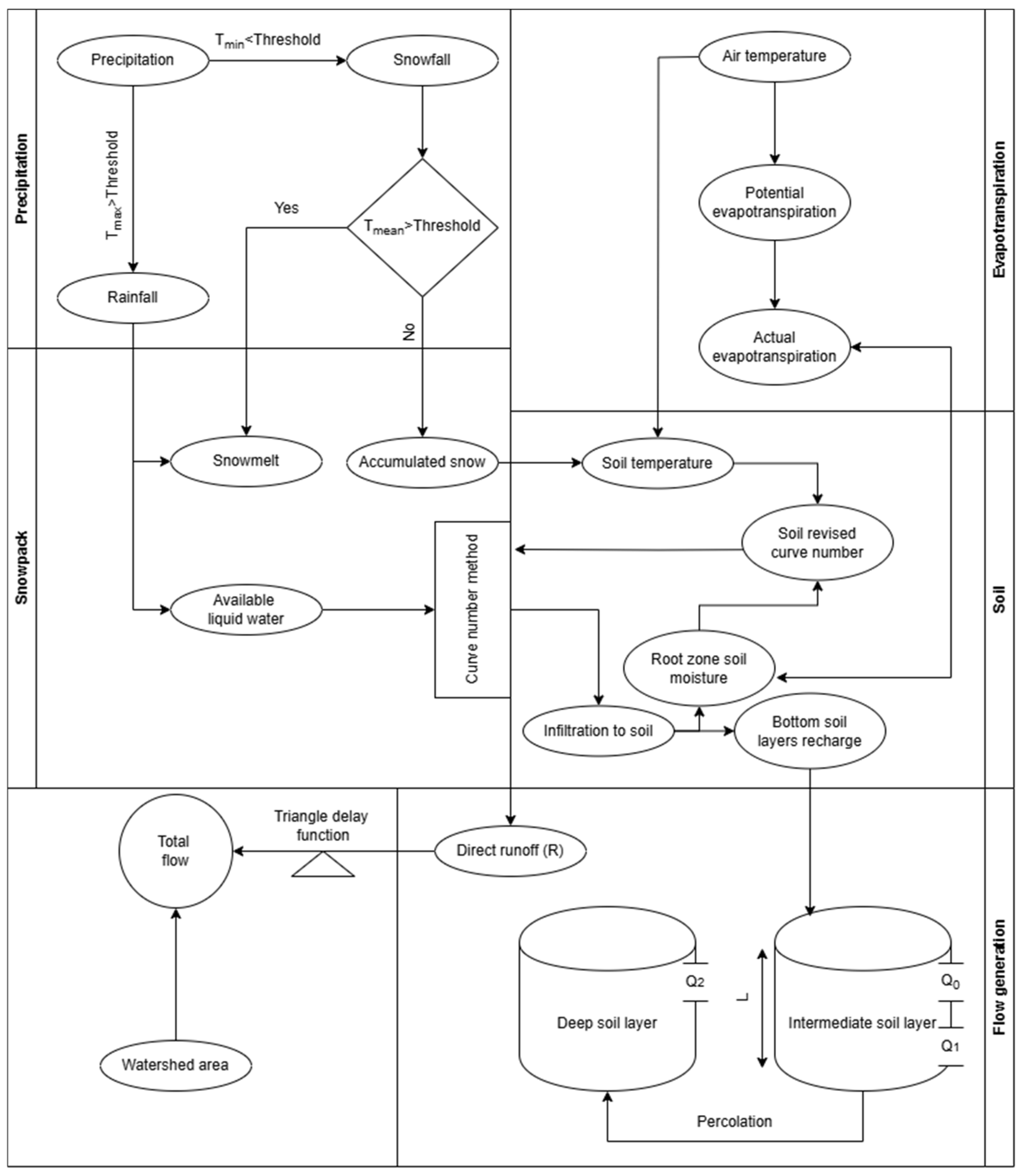
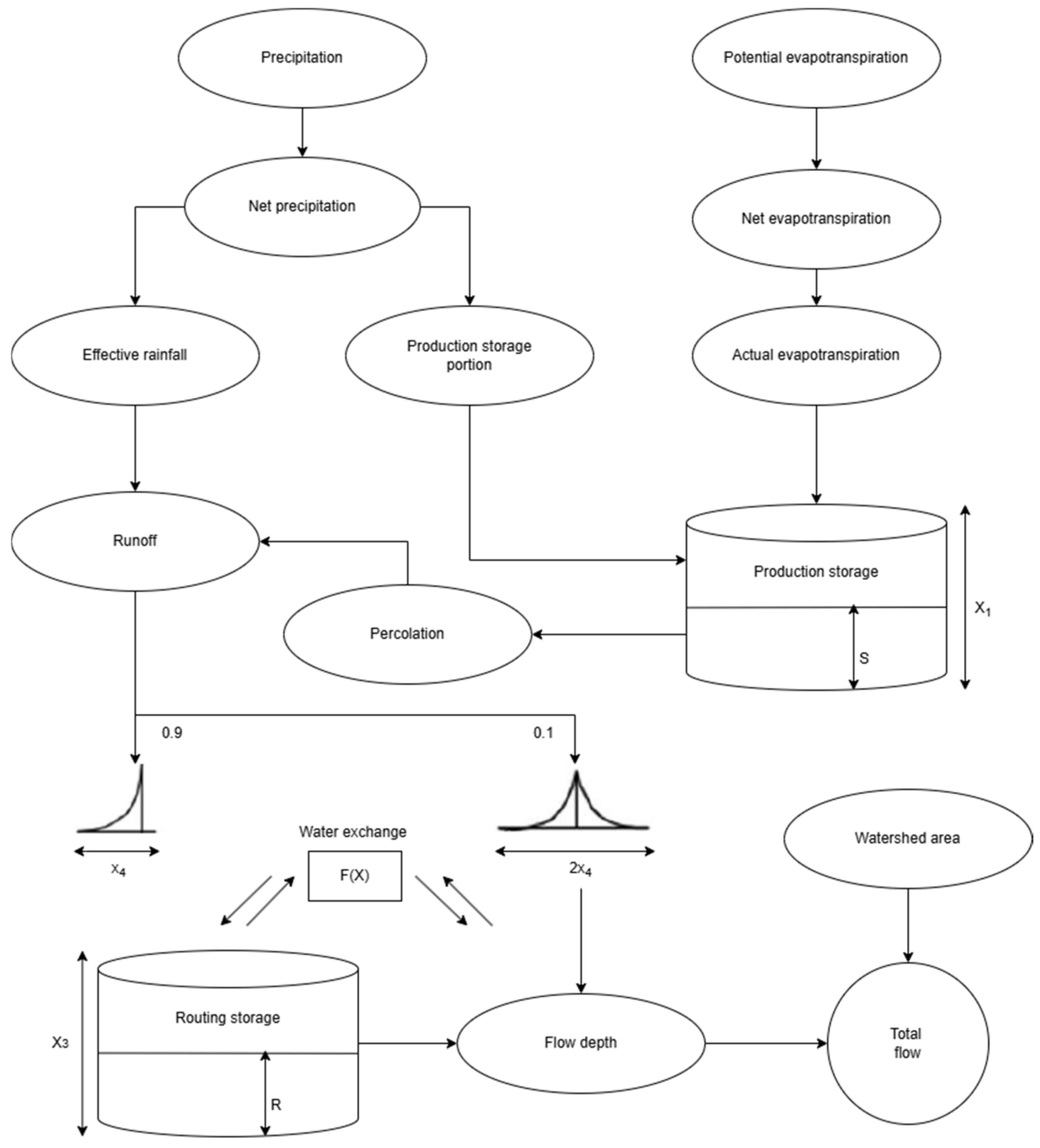
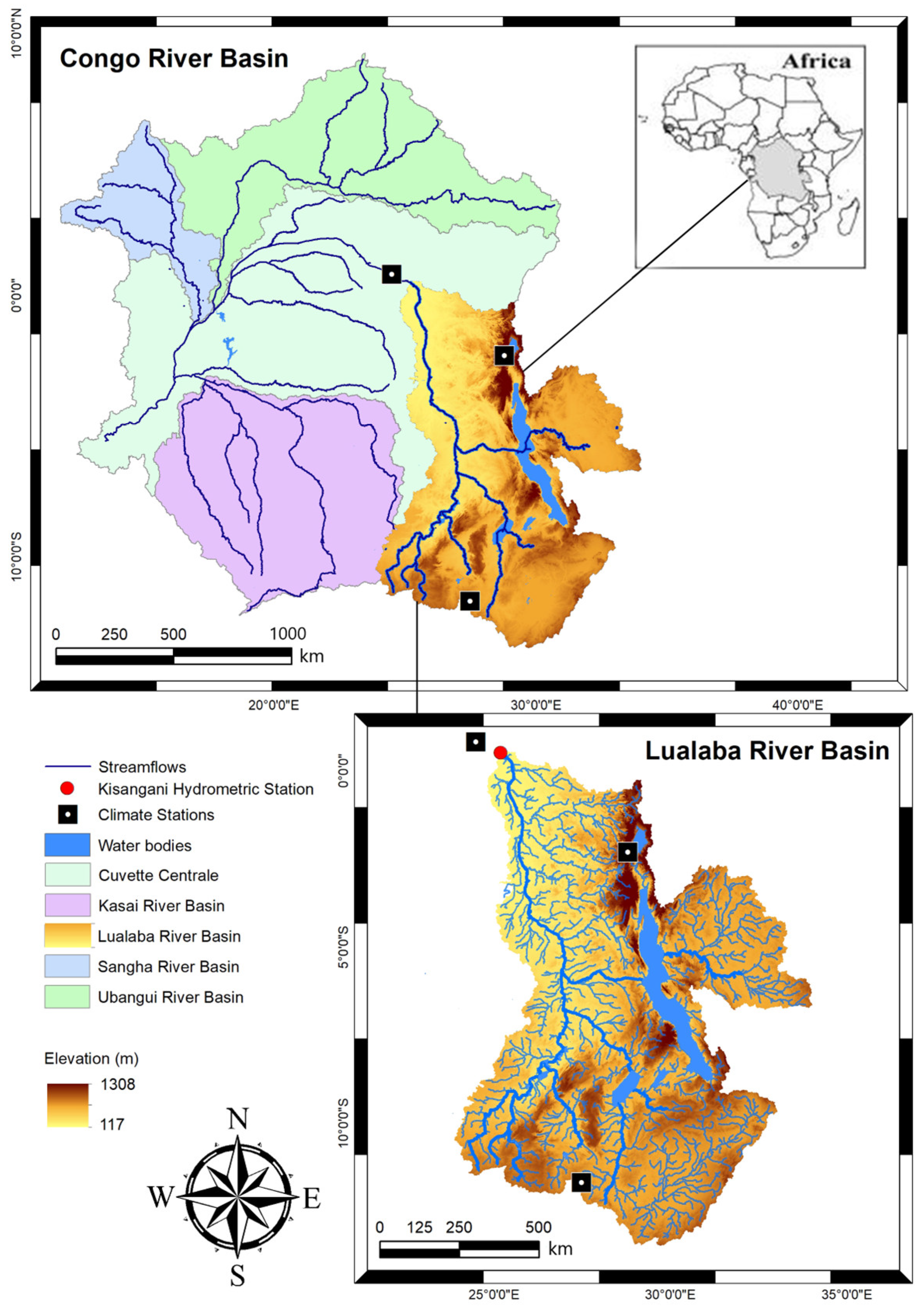
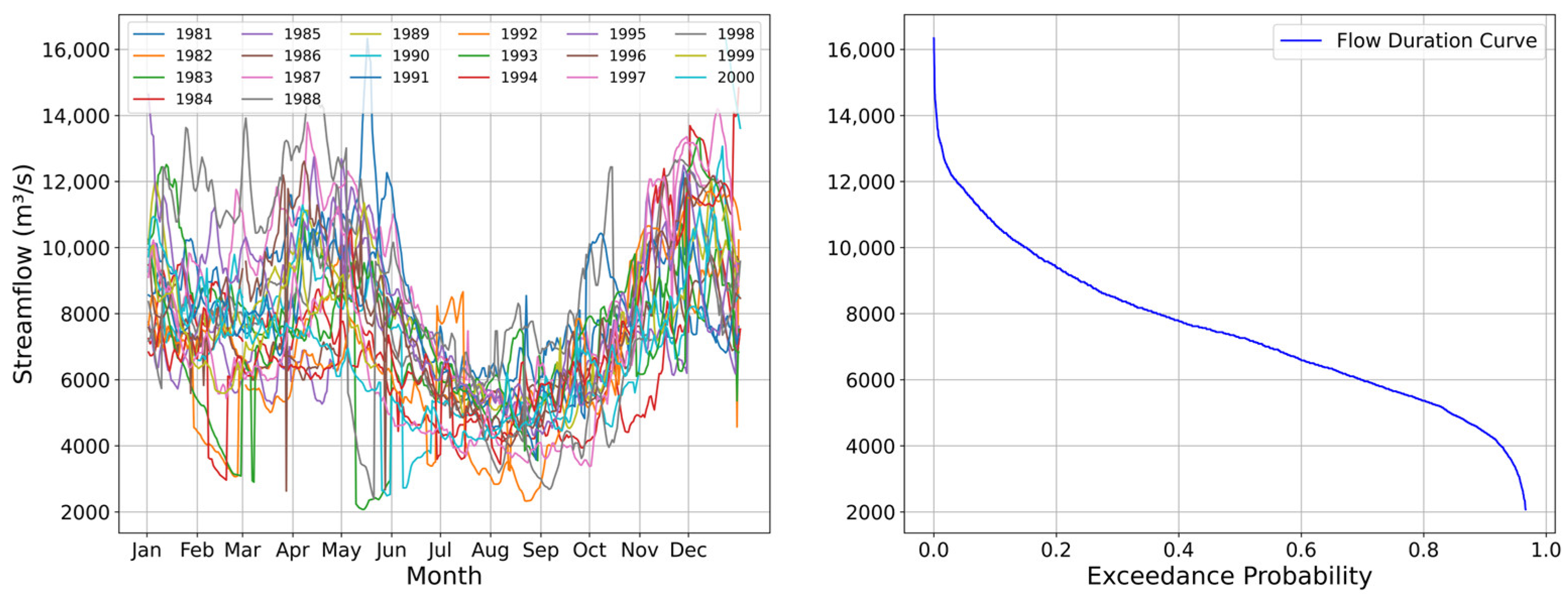
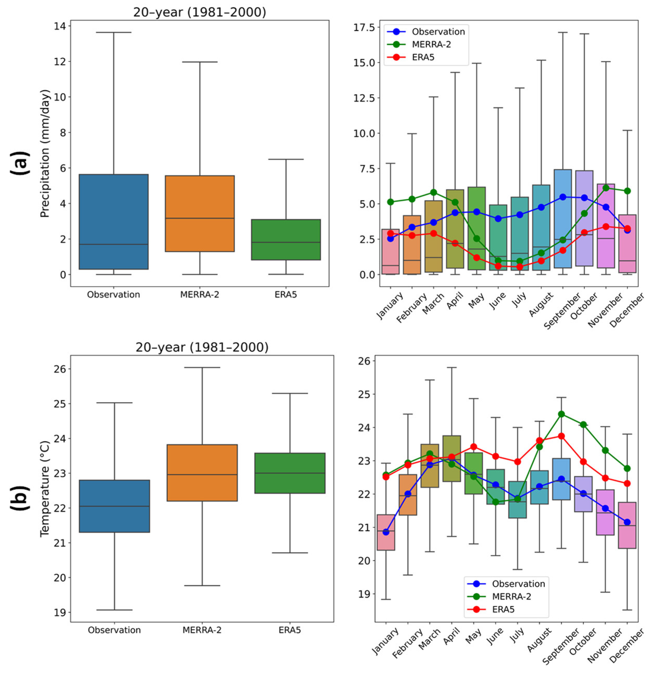


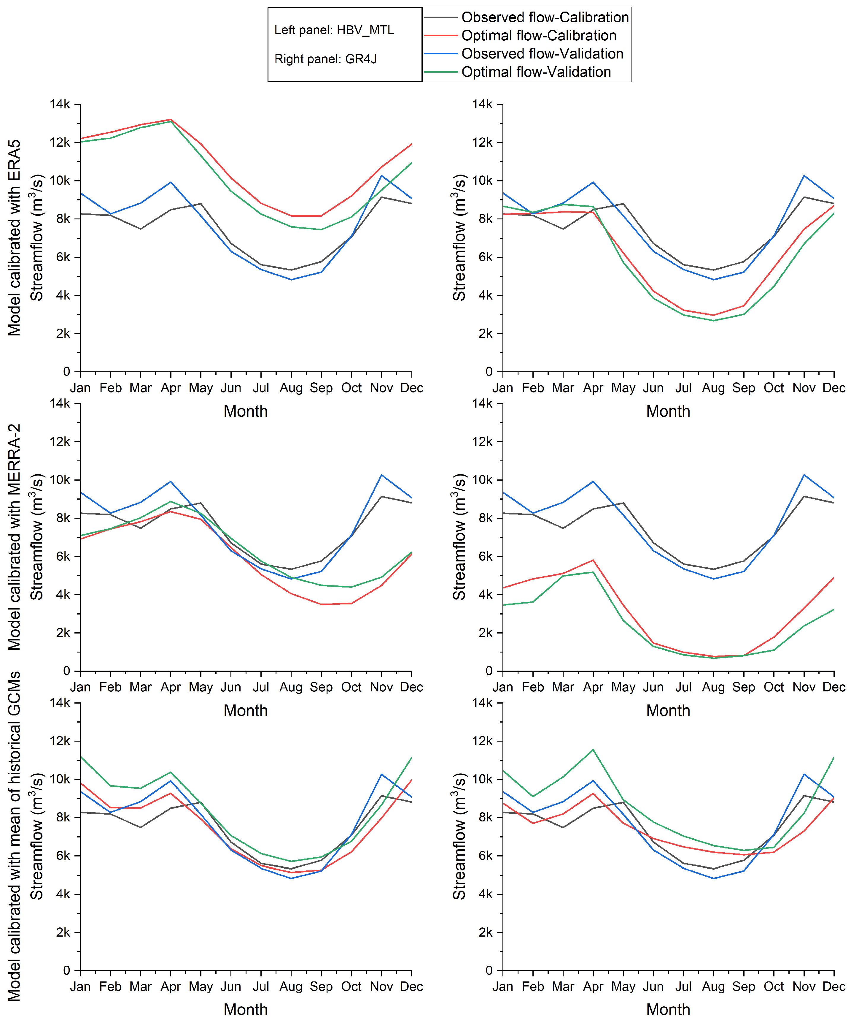
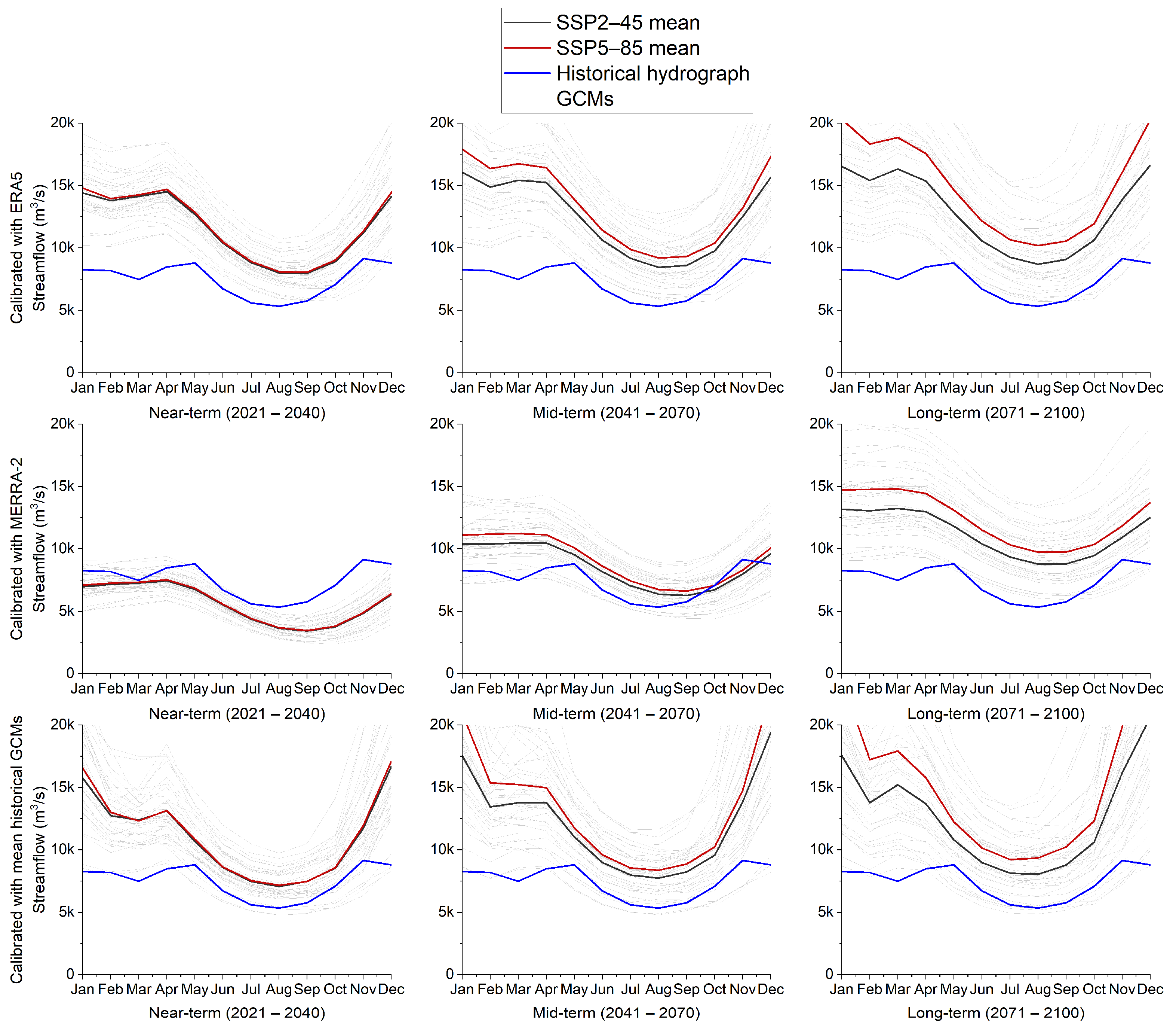

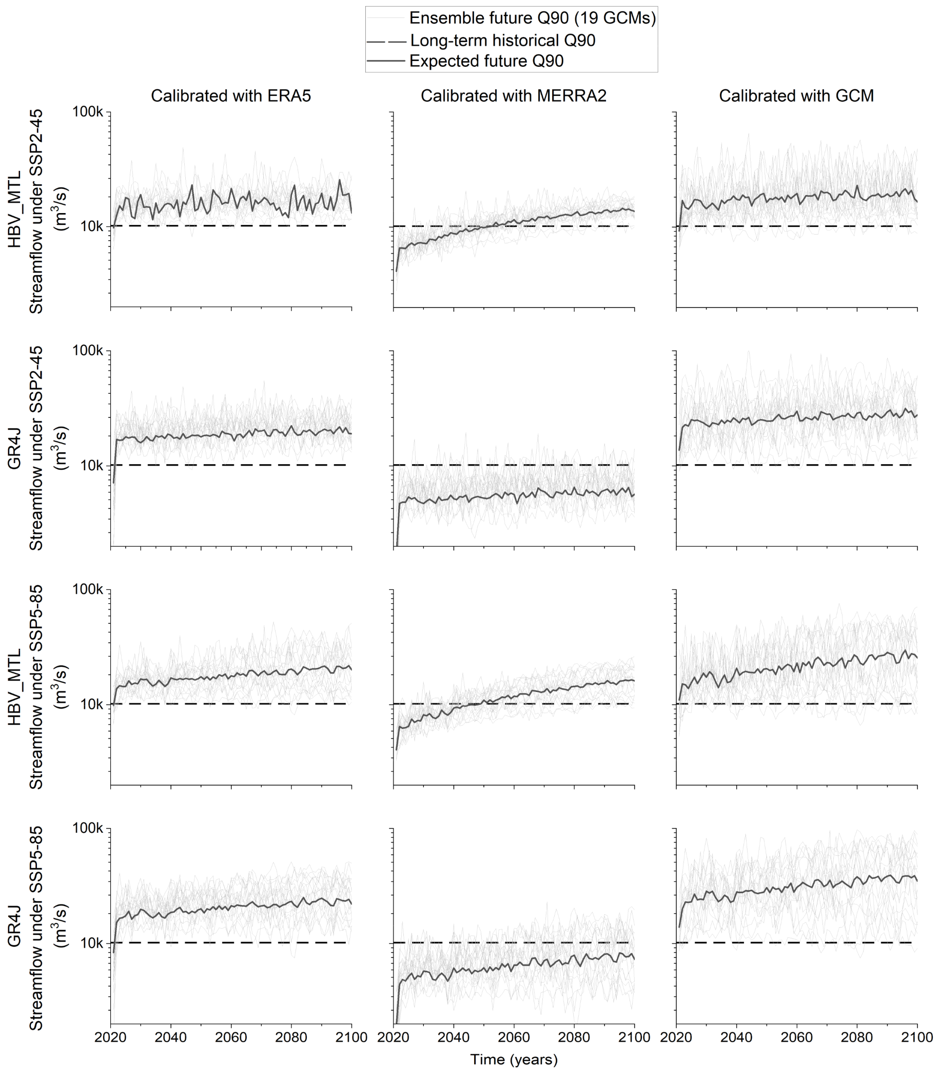
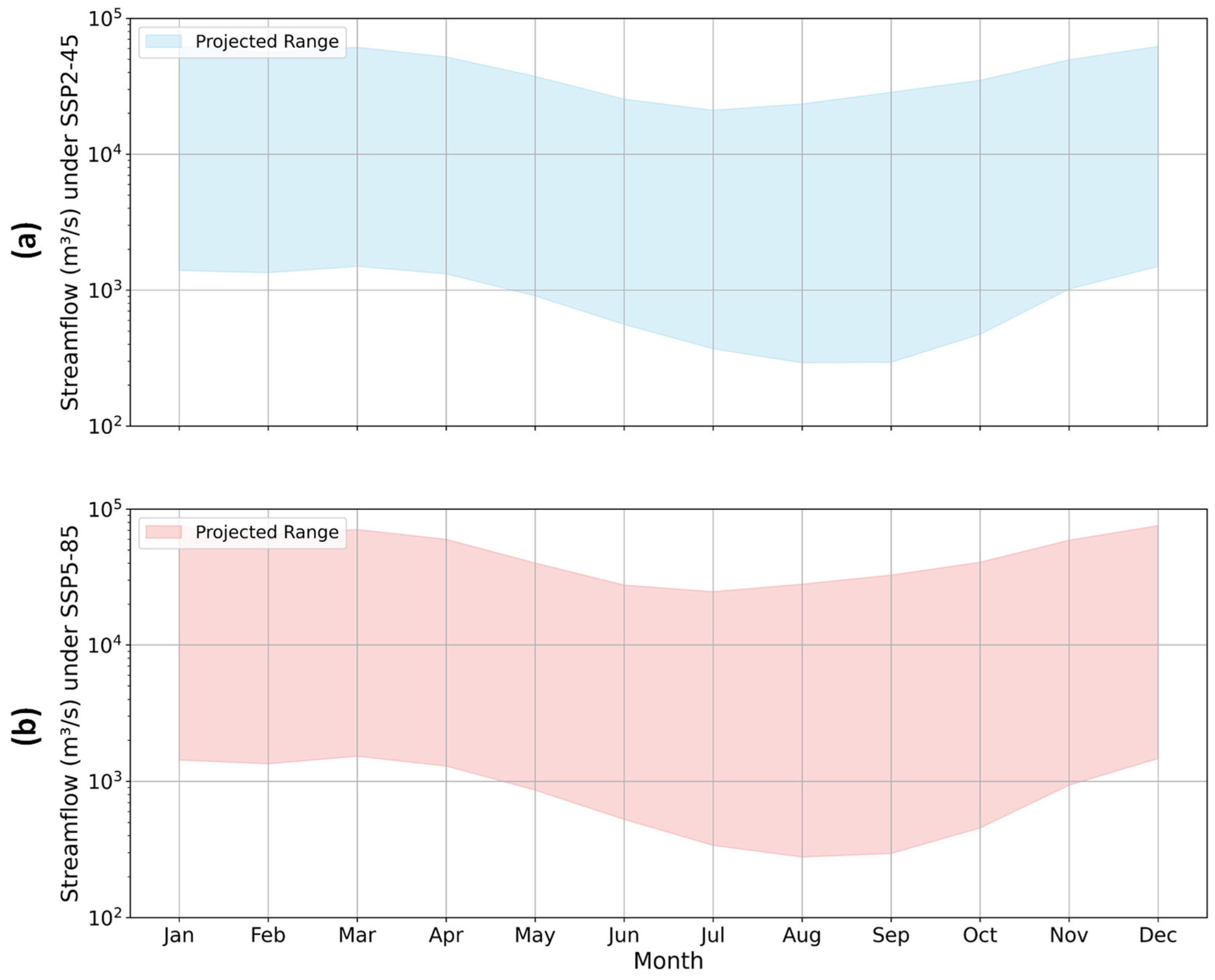
Disclaimer/Publisher’s Note: The statements, opinions and data contained in all publications are solely those of the individual author(s) and contributor(s) and not of MDPI and/or the editor(s). MDPI and/or the editor(s) disclaim responsibility for any injury to people or property resulting from any ideas, methods, instructions or products referred to in the content. |
© 2024 by the authors. Licensee MDPI, Basel, Switzerland. This article is an open access article distributed under the terms and conditions of the Creative Commons Attribution (CC BY) license (https://creativecommons.org/licenses/by/4.0/).