Abstract
The potentially destructive flooding resulting from rain-on-snow (ROS) events motivates efforts to better incorporate these events and their residual effects into flood-related infrastructure design. This paper examines relationships between measured streamflow surges at streamgages across the Western United States and the meteorological conditions preceding them at SNOTEL stations within the same water catchment. Relevant stream surges are identified using a peak detection algorithm via time series analysis, which are then labeled ROS- or non-ROS-induced based on the preceding meteorological conditions. Both empirical and model-derived differences between ROS- and non-ROS-induced stream surges are then explored, which suggest that ROS-induced stream surges are 3–20 percent larger than non-ROS-induced stream surges. Quantifying the difference between ROS and non-ROS-induced stream surges promises to aid the improvement of flood-related infrastructure design (such as culverts) to better guard against extreme flooding events in locations subject to ROS.
1. Introduction
Rain-on-snow (ROS) events occur when rain falls on the existing snowpack [1], often leading to substantial snowmelt and occasionally resulting in dangerous amounts of water runoff. The excess runoff resulting from ROS events is generally the result of soil saturation levels being too high to absorb new moisture combined with snowmelt caused by warm temperatures and high humidity accompanying rainfall [2]. If the combined rainfall and snowmelt produced by an ROS event is large enough to cause flooding, it is referred to as an ROS event with flood-generation potential [3]. Although not all ROS events possess flood-generation potential, those that do pose an immediate concern because of the catastrophic damage caused by ensuing floods on local infrastructure. The concern surrounding ROS events with flood-generation potential is also supported by an observed increase in their frequency over the past 50 years with rising global temperatures due to climate change [4].
There are many existing methods that define the necessary weather conditions for an ROS event to occur, all of which involve some nominal amount of precipitation falling on snowpack. Specific variables used to provide these conditions relate to snowpack in and outflow (e.g., temperature, precipitation, snowmelt, snow water equivalent (SWE), etc.). Mazurkiewicz et al. (2008) [5] required there to be at least 0.254 mm of precipitation falling on snowpack over a 24 h period (divided into three-hour time steps) in order to qualify as an ROS event. Expanding the time window, Freudiger et al. (2014) [3] employed a “3 mm over 6 days threshold” when screening for ROS events with flood generation potential. In another example, the methodology of Musselman et al. (2018) [6] focused on ROS events with flood-generation potential, described in detail in Section 2.4. We note some of the differences in these ROS definitions stem from differences in geographical and climatological contexts. For example, two of these studies focused on the Western United States [5,6], while one focused on Central Europe [3]. Further, each study used different types of data, including historical in situ measurements [5], historical reanalysis data [3], and model-based climate simulations [6]. Despite these differences, these studies provide themes for identifying ROS events with flood-generation potential that inform our current work, as will be explained in the following sections.
Snowmelt is a less commonly reported meteorologic variable that is often difficult to precisely measure. Yan et al. (2018) [7] proposed the use of next-generation intensity duration frequency curves—a recently adapted modeling method used in hydrologic design to accommodate “extreme hydrometeorological events” in locations with heavy snowfall—to estimate precipitation and the resulting “water available for runoff”, or snowpack drainage/melt. They calculate snowmelt directly by examining daily fluctuations in precipitation and SWE within the snowpack to determine its net water content. This calculation is useful because recorded snowmelt measurements are difficult to directly obtain.
One weather-related variable excluded from Musselman et al. (2018) [6]’s ROS classification approach, but included in a number of other approaches, is air temperature. Temperature often serves as a primary indicator for distinguishing between rain and snowfall; however, despite the freezing point being at 0 °C, precipitation type is also influenced by factors like elevation and various other location-dependent conditions. Research on phase partitioning methods to improve the accuracy of making this distinction was discussed by Harpold et al. (2017) [8], who stated that increased accessibility of more sophisticated methods than those available currently is necessary to accurately determine phase partitions. Wang et al. (2019) [9] suggested using wet-bulb temperature as an alternative to near-surface air temperature to differentiate between rain and snowfall since the latter tends to underestimate snowfall in drier regions. Due to the ambiguity in using temperature to distinguish between precipitation as rain and snowfall, ROS classification methods relying on snowpack water content fluctuation are considered somewhat more reliable than methods only employing temperature thresholds.
Much research has been conducted throughout the past several decades to investigate how snowpack characteristics fluctuate during ROS events. Heggli et al. (2022) [10] discussed modeling weather and snowpack conditions for ROS events in order to inform snowpack runoff decision support systems at the site where snowfall occurs and “consider[s] the potential for terrestrial water input from the snowpack”. Wayand et al. (2015) [11] focused on how topography, vegetation, and storm energy influence melt from snowpack during ROS events. Floyd and Weiler (2008) [12] examined snow accumulation measurements and ablation dynamics in ROS events with a focus on snowpack, mentioning how ROS “is the primary generator of peak flow events in mountainous coastal regions of North America”. Würzer et al. (2016) [13] also called out the large peakflow magnitudes produced by ROS events in mountainous areas in the past. Both Wever et al. (2014) [14] and Singh et al. (1997) [15] explored how rainfall, snowmelt, SWE, soil temperature, and additional weather parameters impact runoff observed at snow measurement stations. These studies made valuable contributions to a deeper understanding of snowpack behavior during ROS events, many of them mentioning impacts on streamflow, but none of them directly addressed the impact of ROS on streamflow.
The limited research that exists linking ROS events to streamflow responses predominantly focuses on modeling and predicting streamflow behavior. For example, Rücker et al. (2019) [16] discussed the effects of snowpack outflow on streamflow after ROS events, factoring in the influence of vegetation in their study analyzing data from 2017 and 2018 at several locations in Switzerland. Further, Surfleet and Tullos (2013) [17] investigated the correlation between ROS precipitation events and peak daily flow events in Oregon. Their findings projected a decrease in ROS events leading to high stream peakflows at lower and mid-level elevations, alongside an increase at higher elevations, as climate change perpetuates rising global temperatures. Myers et al. (2023) [18] investigated the impact of ROS events on the hydrology of the North American Great Lakes Basin under climate change, finding a significant reduction in melt in warmer regions but minimal change in colder areas. Additionally, their study highlighted the increasing proportion of rainfall over snowfall, affecting snowpack formation and suggesting implications for freshwater ecosystems and human activities reliant on snow. These studies emphasize the importance of quantifying the magnitude of ROS impacts—since there are many areas across the world with high flood risk due to elevation and changing climate conditions—but none of them quantify the impact of ROS events on flooding in comparison with flooding produced in non-ROS scenarios.
Quantifying increases in streamflow accompanying ROS events has the potential to not only improve understanding of characteristic ROS magnitude in comparison with typical floods but also influence culvert and infrastructure design in an engineering setting. The Hydrologic Engineering Center Hydrologic Modeling System (HEC-HMS), built by the US Army Corps of Engineers, is software “designed to simulate the complete hydrologic processes of dendritic watershed systems” [19]. This engineering tool is used by engineers to simulate hydrologic conditions within a watershed basin and generate predictions of runoff volume and flow [20]. An estimated flood surcharge associated with ROS events would allow engineers using HEC-HMS to adjust simulated flow rates to more accurately model the output of ROS-induced floods and appropriately adjust infrastructure design in at-risk areas.
The remainder of this paper explores temperature, snowpack, and precipitation conditions that precede recorded stream surges in mountain locations across the Western United States. Our unique approach links lower elevation stream gages to higher elevation snow measurement locations, rather than only observing the response of snowpack. To accomplish this, we
- Create a dataset linking historical streamflow peaks across the Western United States to spatially relevant weather conditions,
- Use generalized additive models (GAMs) to represent both ROS and non-ROS-induced peak surges at a regional scale, and
- Examine the differences between ROS- and non-ROS-induced surge representations to quantify ROS impact on streamflow.
Modeling this relationship provides us with a better quantitative understanding of the difference between these two characteristic flood types, allowing infrastructure designers to better anticipate and prevent catastrophic flood damage from occurring in areas vulnerable to ROS-induced flooding.
The remainder of this paper proceeds as follows: In Section 2, we give an explanation of the Western United States streamflow/weather data cleaning and preparation processes as well as the details behind the formation of a streamflow peak dataset. In Section 3, we use GAMs and other machine learning (ML) models to represent streamflow surges from the peak dataset formed in Section 2 and examine the distribution of ROS- to non-ROS-induced surge ratios. In Section 4, we discuss conclusions and areas for future work.
2. Methods
A primary contribution of this paper is a new dataset relating observed surges in streamflow to the weather conditions that preceded the surge. We then classify those weather conditions as ROS or non-ROS-based on variable thresholds described later in this section. To create the dataset, we aggregate streamflow measurements and weather data based on watershed boundaries. The dataset is then used to compare surge size in ROS and non-ROS-induced floods. Table 1 describes the data sources used to obtain the relevant variables. Streamflow, SNOTEL, and PRISM data are accessed through functionality available in the rsnodas package [21]. Data collection is limited to the area encompassed by the Western United States, including the states of Arizona, California, Colorado, Idaho, Montana, Nevada, New Mexico, Oregon, Utah, Washington, and Wyoming.

Table 1.
Data sources used in the creation of the stream surge dataset.
Our primary interest in the streamflow measurements is identifying peaks, or surges, in streamflow. We employ the cardidates R package to identify peaks, which contains the functionality to detect peaks within times series data [26]. The raw streamflow measurements are available at both daily and sub-hourly frequencies, but are often reported on irregular 15-min intervals with stretches of missing values. It is possible that these intervals of missing measurements are sometimes the result of flow rising to unusually high levels, causing gage sensors to malfunction [27,28]. In order to perform peak detection, we require that the data resemble a complete time series, with non-missing measurements reported at regular time intervals. To correct the time series intervals while still preserving the temporal scale of the data, we retain hourly maximum streamflow measurements and linearly interpolate any missing values in the hourly time series using the neighboring streamflow measurements. While some streamgages required multiple attempts to successfully download their measurements, our data download process results in the collection of 22.1 million hourly streamflow measurements from 2348 of 2586 possible streamgages.
2.1. Peak Detection and Baseflow Calculation
Once the data are appropriately organized, we use an application of the peakwindow() function from the cardidates R package to detect peaks within the data based on a user-specified threshold. Whenever possible, we use predefined flood stages as this threshold. The National Weather Service defines flood stage as “the stage at which overflow of the natural banks of a stream begins to cause damage in the local area from inundation (flooding)” [22]. Predetermined flood stages are published online by the USGS for 737 of the 2586 streamgages originally involved in our study (28.5 percent). Flood stages for the remaining 1849 gages are estimated using a multiplier based on each station’s maximum recorded streamflow measurement. The multiplier is defined as the median ratio between the maximum recorded streamflow measurement and the recorded flood stage from the previously described set of 737 stations. The ratio between the maximum recorded streamflow measurement and the flood stage varies widely from 0.05 (i.e., flood stage is 5 percent of the maximum recorded streamflow measurement) to more than 10 (i.e., flood stage is 10 times the maximum recorded streamflow measurement). That said, the interquartile range of these ratios falls in a relatively tight range of 0.44 to 0.88, suggesting that a typical flood stage tends to be between 44–88 percent of the maximum recorded streamflow measurement. With this in mind, we select the median value of 0.67 as the multiplier to estimate flood stages as a function of maximum recorded streamflow. In other words, for stations lacking pre-defined flood stages, stream surges are only retained if the surge is larger than 66 percent of the maximum recorded streamflow measurement. The use of this multiplier attempts to strike a balance between focusing on streamflows with flood generation potential, while still preserving an adequate sample size for analysis. One limitation of this approach is the dependence upon the maximum recorded streamflow measurement, which, while easy to obtain, is sensitive to outliers. While our results suggest a reasonable balance between flood-stage-defined stream surges and flood-stage-estimated stream surges, future work should consider alternative methods for imputing flood stage thresholds.
The cardidates package documentation [26] describes how the peakwindow() function operates in two steps: (1) peak identification and (2) peak refinement. We summarize their description of the peak detection process in the context of this specific project as follows:
- Peak identification: Every streamflow value that exhibits a higher value than at the timestamps directly before and after its occurrence is identified as a peak.
- Peak refinement: The list of identified peaks is refined by defining ‘subpeaks’ that are excluded from the finalized peak list. Subpeaks are characterized by either having a height that falls below the flood stage threshold at their corresponding streamgage or by not having a sufficiently large trough, or pit, between neighboring peaks. This refinement process is repeated until there are no more subpeaks.
After defining existing/estimated flood stages for each streamgage, we implement the peak detection algorithm using the peakwindow() function and identify peaks at 2199 of the 2348 available streamgages using each gage’s full period of record. We detect a total of 60,811 peaks between all the streamgages. Of these 60,811 peaks, 55,207 are reported at streamgages with estimated floodstages (90.8 percent). The majority of the 2199 gages reporting peaks have 30–40 years worth of data and began recording streamflow measurements at the subhourly level between 1986 and 1990, the first recorded date being 1 January 1980. Note that this study treats each stream surge as a unique and independent observation, which means that streamgages with longer periods of record have a greater influence on model results.
In order to examine differences in streamflow surges between ROS and non-ROS peaks, we obtain a baseflow () measurement preceding each peakflow () measurement and define stream surge (g) in Equation (1) as
Peakflow measurements for each streamgage are reported by the peak detection algorithm along with the timestamp. We calculate baseflow by finding the median of hourly streamflow measurements at the relevant streamgage in the two-week period prior to the stream surge peak. For instances where two peaks occur in a time period shorter than two weeks, we adjust the algorithm to use the median of the streamflow measurements in the time between the two neighboring peaks to describe the baseflow of the latter peak.
2.2. Weather Data
Weather data measurements are obtained at a daily level for 808 SNOTEL stations across the 11 states of interest. The specific variables we use to inform ROS flood classification and surge representation include the following:
- Temperature (Temp in °C)
- Precipitation (Precip in mm)
- Snow Depth (SD in cm)
- Snow Water Equivalent (SWE in mm)
- Soil Moisture (SM as percentage)
- Elevation (Elev in m)
- Snowmelt (Melt in mm)
SNOTEL stations use devices called snow pillows to measure SWE, which describes the water content available in the snowpack [29]. Melt () is not a variable reported directly by SNOTEL stations, so we calculate it using Yan et al. (2018) [7]’s method with measured Precip and SWE. This calculation is performed as follows:
where represents SWE, p represents Precip, and q represents day. Equation (2) assumes that measured Precip is equivalent to the increase in water content of the snowpack on days with no snow melt. Any bias in measurements of Precip or SWE would thus be reflected in this calculation. Future research should compare this calculation to modeled estimates of snow melt such as those available in the Snow Data Assimilation System (SNODAS) [30]. This snow melt measurement is used in the Musselman et al. (2018) [6]’s ROS classification framework described previously.
2.3. Associating Streamgages and SNOTEL Stations
The USGS’s Hydrologic Unit Code (HUC) system divides the United States into a set of drainage basins at six different spatial scales, ranging from continental (HUC 2) to local (HUC 12). A drainage basin, or watershed, is an area of land that captures precipitation and channels it into a creek, river, or stream, eventually leading to the ocean [31]. In order to associate the streamgages and SNOTEL stations in our dataset, we group them together by HUC 8 watershed boundaries. We only retain measurements contained in watersheds that have at least one SNOTEL station and at least one streamgage. Connecting streamgages and SNOTEL stations in this way assumes that measured water at SNOTEL stations will flow to the streamgages existing in the same HUC 8 basin. After associating streamgages and SNOTEL stations by HUC region, only 7807 of the 60,811 (13 percent) peaks remain for analysis at 1279 unique streamgages. Of these remaining peaks, 4977 (64 percent) are reported by streamgages with estimated flood stages. This considerable post-association decrease as well as intermediary decreases in usable SNOTEL station and streamgage counts are shown by Table 2. Despite the data loss, exploration of ROS in HUC 8 watersheds containing SNOTEL stations allows us to target streamgages in mostly mountainous areas prior to flood control measures (i.e., dams), which are likely the streamgages most sensitive to fluctuations from ROS events.
Table 2.
SNOTEL station and streamgage counts at each step in the data refinement process.
2.4. Daily ROS Event Classification
Recall the many different ways of defining an ROS event in Section 1. In this study, we employ the Snowmelt calculation utilized by Yan et al. (2018) [7] (and subsequently defined in Equation (2)) in conjunction with Musselman et al. (2018) [6]’s ROS classification approach. We implement this method using historical Precip and SWE values reported by SNOTEL stations. This method requires that the following three conditions be met in order to positively classify an ROS event:
- mm
- mm
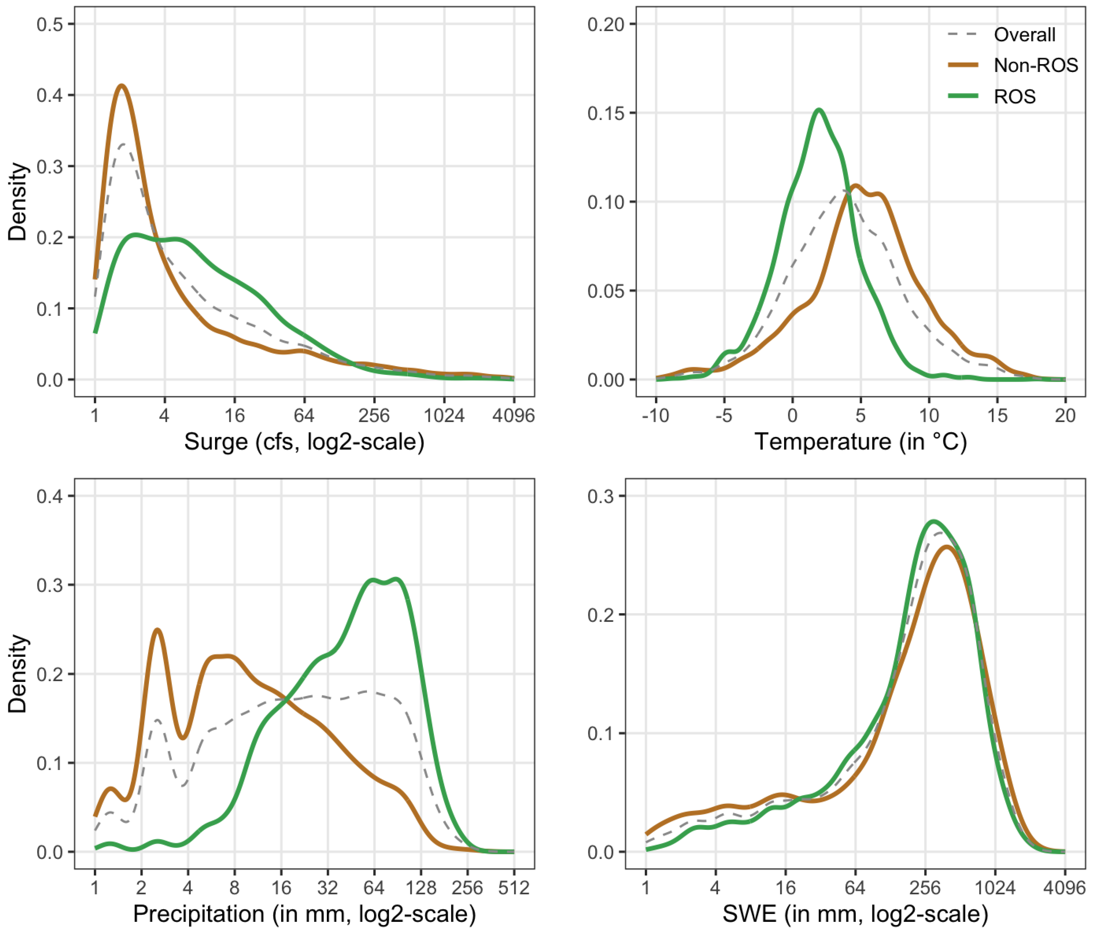
where p is Precip, is SWE, and is Snowmelt. After identifying days when ROS event conditions have been met at individual SNOTEL stations, we determine whether a day qualifies as an ROS event day at the HUC 8 level by requiring that at least half of the SNOTEL stations within a HUC region fulfill the requirements for an ROS event to occur. We then classify peaks as ROS induced if they occur within seven days of an ROS event in their respective HUC region. Of our remaining peaks, 2725 are classified as ROS induced (34.9 percent) and the remaining 5082 (65.1 percent) as non-ROS-induced. Figure 1 shows the distributions of surge magnitude in ROS- and non-ROS-induced floods classified using this method. We see that non-ROS-induced surges tend to be considerably smaller than those that are ROS induced, and that the overall surge distribution most closely resembles the distribution of non-ROS-induced surges.
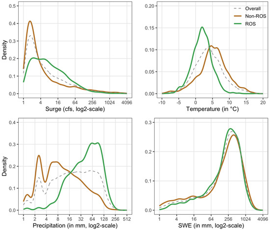
Figure 1.
Densities of ROS vs. non-ROS classified streamflow surge, Temp, Precip, and SWE measurements in comparison with the overall distributions of these variables.
We also explore the different distributions of the weather conditions preceding a stream surge for both ROS and non-ROS events in Figure 1. The distributions of Temp, Precip, and SWE are shown to highlight differences between ROS and non-ROS behaviors. We see that temperatures for ROS-induced peaks tend to be around 2.8 °C lower than those that are non-ROS-induced, possibly due to the time periods throughout the year in which both peak types are more likely to occur. The left skew in ROS compared to the right skew of the non-ROS Precip measurements indicate that for surges classified as ROS induced, Precip measurements preceding the surge tend to be substantially larger. ROS and non-ROS follow similar distributions for SWE.
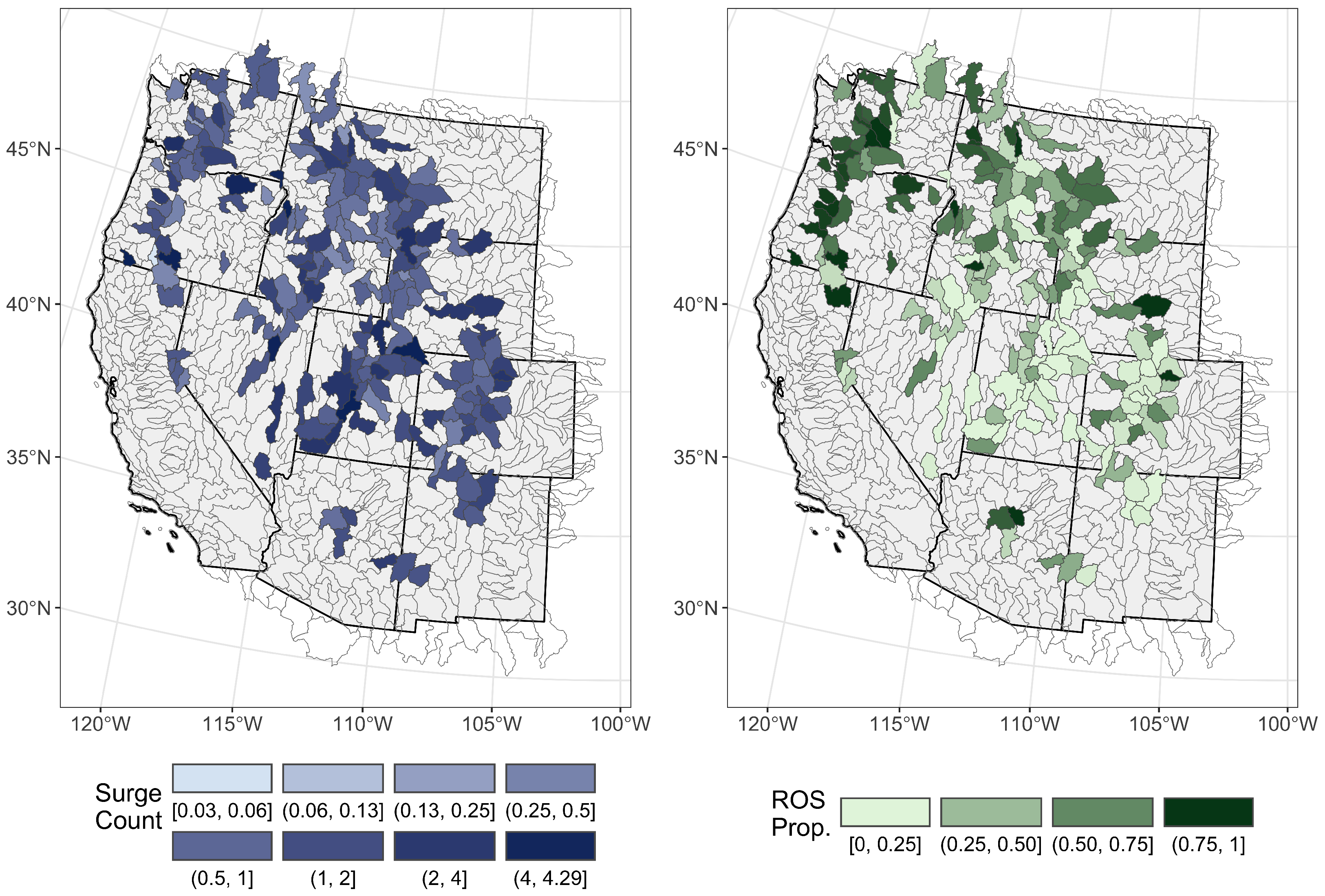
However, Figure 1 ignores the spatial structure inherent in the data, as ROS events do not occur at the same rate across the Western United States. Figure 2 visualizes the spatial distribution of surge counts and relative surges attributed to ROS events in the region of interest. We see that there is a higher proportion of ROS surges in the Northwest, confirming that ROS events tend to occur more frequently in northern mountainous regions near the coastline [6]. It also shows that the overall surge count per year by HUC 8 region does not follow a clearly identifiable pattern across the region of interest.
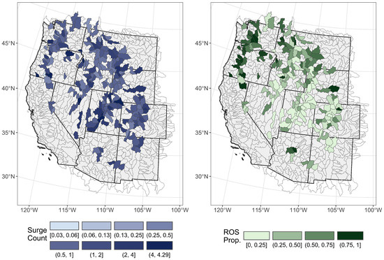
Figure 2.
Choropleth maps comparing overall surge count per year in each HUC region (left, log2 scale) to the proportion of the surge count that is ROS induced (right, linear scale).
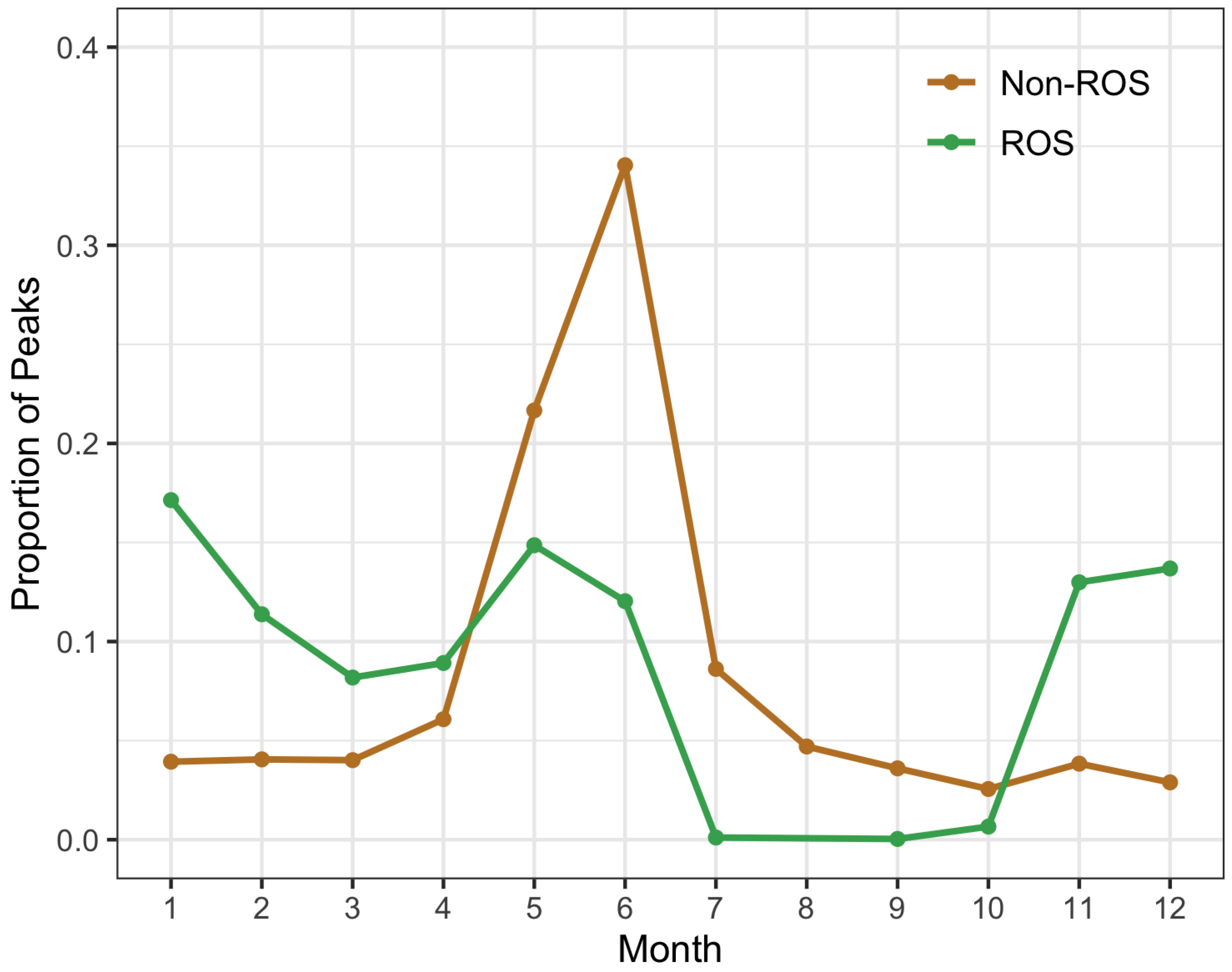
Figure 3 shows the frequency of ROS- and non-ROS-induced surges by month. We observe that the majority of non-ROS-induced flooding occurs during the spring and summer months, specifically in May and June, likely in the form of spring runoff. In contrast, ROS-induced floods seem to occur in roughly equal proportions from November to January as well as May.

Figure 3.
Proportions of total peaks occurring in each month by ROS classification.
We next examine the distribution of the ratios of ROS vs. non-ROS-induced surges. This ratio is calculated for an individual streamgage in Equation (3):
where r is the ratio of surges, is the station-level median of all ROS-induced surges, and is the station-level median of all non-ROS-induced surges. Only the 245 streamgages with at least two non-ROS and ROS peaks are considered in the final distribution. Due to our relatively small sample size of peaks and the inherently sensitive nature of ratio calculations, tends to be overly influenced by outlier observations. Figure 4 shows the full range of these empirical ratios, with the largest and smallest outliers indicating, respectively, that there were streamgages whose median ROS surges tended to be 30 times larger and 50 times smaller than their median non-ROS surges.
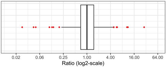
Figure 4.
Boxplot showing the full range (log scale) of empirical ratios of ROS-induced surge to non-ROS-induced surge measurements at streamgages with qualifying peaks. Values above one indicate that ROS-induced surges tend to be larger than their non-ROS-induced counterparts and vice versa.
2.5. Database Description
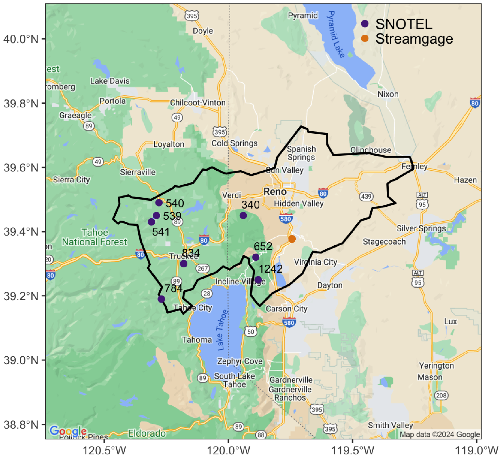
For each of the 7807 remaining flood peaks in our analysis, we link weather variables to the streamgage’s peak occurrence by calculating summaries of measurements from SNOTEL stations located in the same HUC region for the 5 days prior to the peak day. We assume the dependence of streamflow response upon the accumulation of Precip, SD, etc. during the 5 days leading up to the peak. The choice of five days is similar to the six-day window explored by Freudiger et al. (2014) [3] and is intended to account for the fact that it may take several days for streamflow to respond to an ROS event occurring in a separate part of the same watershed. That said, future work should determine the sensitivity of the ROS classification to variations in the period of time preceding a stream surge that is considered for ROS classification. For each weather variable, values for all SNOTEL stations within the relevant HUC region over the given time period are collected, and the HUC-level median of the following summary statistics is calculated separately for each station: mean, median (station-level), minimum, and maximum. The sum of Precip over this time period is also calculated. The overall median value for the entire HUC region for each summary statistic is then added to the data frame containing peak information. We include an example of this aggregation for a single ROS-induced streamflow peak near Reno, Nevada on 10 February 2017. The map in Figure 5 shows the spatial distribution of the SNOTEL stations and streamgage within the HUC 8 boundary.
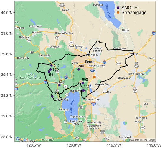
Figure 5.
Map of HUC 16050102 with eight SNOTEL stations (IDs: 540, 1242, 809, 539, 784, 340, 541, 652—sorted by Elevation) and one streamgage (ID: 10349300).
We show the aggregation of data required to connect SNOTEL weather data with the streamgage in Table 3. This example only shows the aggregation for the means of each weather variable to demonstrate the workflow—median, minimum, and maximum measurements are also computed and stored in a similar manner. The ‘HUC’ column in this table represents the specific values appended to this peak observation in the peak data frame. This aggregation is performed for each of the 7807 peaks. Additional relevant variables in the final data frame used for analysis include peakflow, baseflow, surge, ROS classification, and the geographic location (i.e., longitude and latitude) of the streamgage at which peak occurrence is observed. Overall, there are 49 variables associated with each peak observation. A list of all variables and the summaries applied to the weather variables is available in Table 4.
Table 3.
Example of data aggregation by HUC region for a singular peak. Mean measurements are found at each SNOTEL station for the 5 days prior to peak occurrence (stations are sorted by increasing elevation). The ‘HUC’ column contains the HUC-level medians of the station-level mean measurements for each variable and are highlighted in bold. Variables include Temperature (Temp), Precipitation (Precip), Snow Water Equivalent (SWE), Snow Depth (SD), Soil Moisture (SM), Snowmelt (Melt), and Elevation (Elev).
Table 4.
List of variables and their associated statistical summaries included in final dataset.
The final dataset connects weather measurements to streamflow surges through HUC association to establish spatial dependencies, allowing us to meaningfully investigate streamflow response to weather behavior. It also contains information about ROS classification for each peak, which provides us with not only a better understanding of the characteristics of ROS-induced floods, but also a better understanding of the relationship between ROS and non-ROS floods and what distinguishes their behavior. The following section demonstrates an application of this dataset to model differences between ROS- and non-ROS-induced stream surges.
2.6. Model Selection and Tuning
We create generalized additive models (GAMs) for representing stream surge with the intent to provide a more accurate and stable indicator of stream surge differences while controlling for location-specific anomalies. GAMs are an adaptation of a linear model that permits nonlinearity in the prediction of the response variable through the use of data-driven smoothing functions [32]. Due to the highly skewed distribution of surge measurements, we elect to use the log of surge as our response variable.
As an initial step in the modeling process, we determine which of the 37 eligible explanatory variables from the peak dataset are the most important in predicting log-surge through a combination of tests for statistical significance and practical viability. For example, we remove SM percentage measurements from consideration for practical purposes since over 80 percent of peak observations report it as missing. The remaining variables are selected based on their significance and explanatory power, as determined through the manual addition and removal of variables from the candidate models. The initially retained variables for modeling log-surge are summarized in Table 5.
Table 5.
List of variable summaries included in the initial version of the GAM formula. Baseflow, latitude, and longitude do not undergo summarization so the ‘Baseflow (log-transform)’ and ‘Coordinates’ rows are left blank.
In order to introduce the mathematical representation of the simplified GAMs, let u and v be vectors representing a collection of one or more geographic coordinates in (longitude, latitude) format. Further, let u correspond to the geographic location of the streamgage measuring the ith surge and correspond to the unique geographic location of the jth SNOTEL station located in the same HUC region as the related streamgage. Let be the vector of length j containing mean SWE measurements at multiple SNOTEL stations (with locations ) for the 5 days prior to peak occurrence in the relevant HUC region (). Since there are often multiple SNOTEL stations within a HUC region, we summarize over by finding the median, represented by the superscript (m), of the mean SWE measurements from all j SNOTEL stations. Finally, let i indicate the index of the surge in our dataset of flood peaks that this value is calculated for. For example,
represents the median of the mean SWE for a particular stream surge measured at a stream gage in watershed . We use similar notation for median Temp (), mean SD (), and maximum Precip (). The remaining explanatory variables, including baseflow () and the geographic location of the gage (u), are derived from streamgage rather than SNOTEL stations and require no statistical summary prior to inclusion in the model.
Let denote the default smoothing functions used in our model that employ penalized thin plate regression splines [33]. Additionally, let represent isotropic second-order splines on the sphere for modeling any marginal geographic effects [34]. Equation (4) represents our final GAM post the variable selection described in Section 3.
3. Results
3.1. Cross Validation
To validate the accuracy of our GAM, we implement 10-fold cross-validation (CV) at the streamgage rather than observation level. In other words, all observations from a single stream gage are grouped together in the training or test sets in each fold of the CV. We track GAM results when including and excluding SD to see if a simplified model will yield similar results. Table 6 shows the mean squared error (MSE) and mean absolute error (MAE) resulting from 10-fold CV. These results show that the model containing SD performs slightly worse than the model excluding it, though this may be partially explained by the fact that the model including SD has fewer observations available for training and testing. Regardless, the performance suggests that there is little to no benefit in including SD in the GAM model predicting stream surge.
Table 6.
Initial GAM accuracies, both including and excluding SD.
To assess the effectiveness of these GAMs in surge representation, we observe the performance of a null model to compare with the accuracy of the GAM predictions. The null model does not contain explanatory or response variables—it simply provides the global median of the log-surge multiplier we are predicting with the GAMs. After 10-fold CV, this basic model produces a MSE of 3.28 and a MAE of 0.8. Since the fitted GAM excluding SD reduces the MSE by 75 percent and the MAE by 40 percent and the GAM containing SD reduces the MSE by 71 percent and the MAE by 38 percent relative to the null model, we have evidence that both GAMs produce meaningful predictions, and we proceed to further simplify the models without substantial loss in predictive power.
GAM models with fewer variables are easier to deploy and less sensitive to small changes in input data. This motivates us to narrow the model formula down to include just one Temp and one Precip measurement type rather than several different summaries of those two variables, as was the case for the models presented in Table 6. To do this, we create a list of formulas in which we provide all possible combinations of individual Precip and Temp variables while holding the other variables constant. We then fit a GAM with each formula from this list to determine which has the smallest MSE after CV. Results for all variable combinations, both including and excluding SD, are similar in accuracy, with the models using median Temp and maximum daily Precip being the most accurate. The final variables considered in the GAM modeling are median Temp, maximum Precip, mean SWE, log of Baseflow, and geographic location (i.e., latitude/longitude), as was previously shown in Equation (4).
3.2. Station Profiles
The primary purpose of the GAM models is to quantify changes in predicted stream surge for different combinations of variables representing ROS and non-ROS events. Using the final two GAM models (one including SD and one excluding SD), we formulate characteristic profiles for ROS and non-ROS conditions specific to each streamgage. We do this by using the summary statistics shown in Table 7 for each explanatory variable utilized in our GAM. The median annual maximum variable measurement is chosen in several cases to represent what would be considered an “extreme”, though not uncommon, ROS event. In this way, the profile is intended to provide a conservative estimate of the relative difference between ROS- and non-ROS-induced stream surge. A more detailed description of why we choose each specific summary statistic to represent the profiles is given as follows:
- Temp: We use the global medians of non-ROS and ROS classified peaks, since measurements for both scenarios remain somewhat consistent across locations. Unlike other variables, these values are set globally rather than separately for each station.
- Precip: We use the median annual maximum Precip measurement for both non-ROS and ROS-induced peaks because current engineering design practice relies on projections of extreme Precip that do not discriminate between ROS and non-ROS events.
- SD: We use a measurement of zero for non-ROS-induced peaks because an ROS event cannot occur if there is no snow. We then use the median annual maximum SD measurement for ROS-induced peaks because it is representative of a large, though not uncommon, snow accumulation event.
- SWE: We use a measurement of zero for non-ROS-induced peaks and the median annual maximum SWE for ROS-induced peaks, using the same justification that we use for SD.
- Baseflow: We use the median overall baseflow measurement for each streamgage, as it gives a sense of the typical flow at the gage.
Table 7.
Values used to describe characteristic profiles for ROS and non-ROS events.
Table 7.
Values used to describe characteristic profiles for ROS and non-ROS events.
| Variable | ROS | Non-ROS |
|---|---|---|
| Temp | overall ROS median | overall non-ROS median |
| SD | median annual maximum | 0 |
| Precip | median annual maximum | median annual maximum |
| SWE | median annual maximum | 0 |
| Baseflow | overall median | overall median |
| Coordinates | station-specific | station-specific |
3.3. Training the GAMs
With the profiles compiled for each streamgage, we train the GAMs on the original data containing information about each peak and use those trained models to create a dataset containing surge predictions for the characteristic profiles defined for each streamgage. After generating predictions for both the ROS and non-ROS profiles at each streamgage, we calculate the ratio between ROS and non-ROS exponentiated surge multipliers, furthermore referred to as the ROS stream surge ratio (ROSSR). The ROSSR is calculated by streamgage similarly to the empirical surge ratios in Equation (3), but without the aggregation by median, resulting in the following simplified formula:
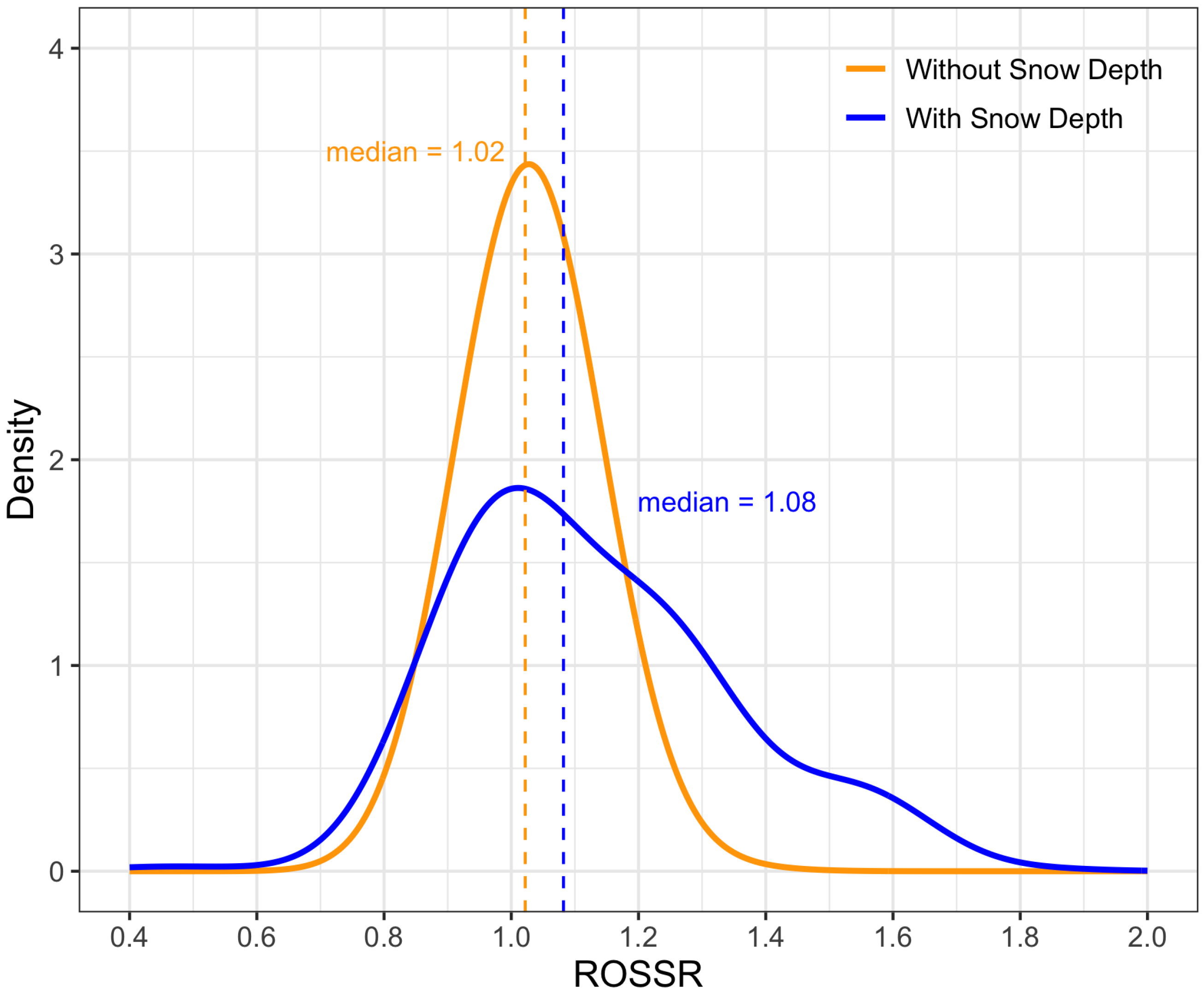
where r is the ratio, is the predicted surge for the ROS profile, and is the predicted surge for the non-ROS profile. The distributions of these ratios from the GAMs both including and excluding SD are used to investigate the general behavior of surges in ROS vs. non-ROS flood peaks, as shown in Figure 6. We see that the GAM excluding SD generates surge predictions for ROS and non-ROS that are more similar to each other than those produced by the GAM containing SD.
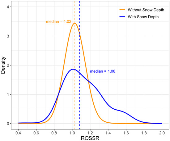
Figure 6.
Distribution of ratios of surge predictions for ROS and non-ROS behavior at streamgages with qualifying peaks for both the GAM with SD and the GAM without.
To better understand the role each term in Equation (4) plays in the predicted surge values, we examine plots of the marginal effects for both GAMs. For simplicity, this paper only shows the marginal effects for the model, excluding SD.
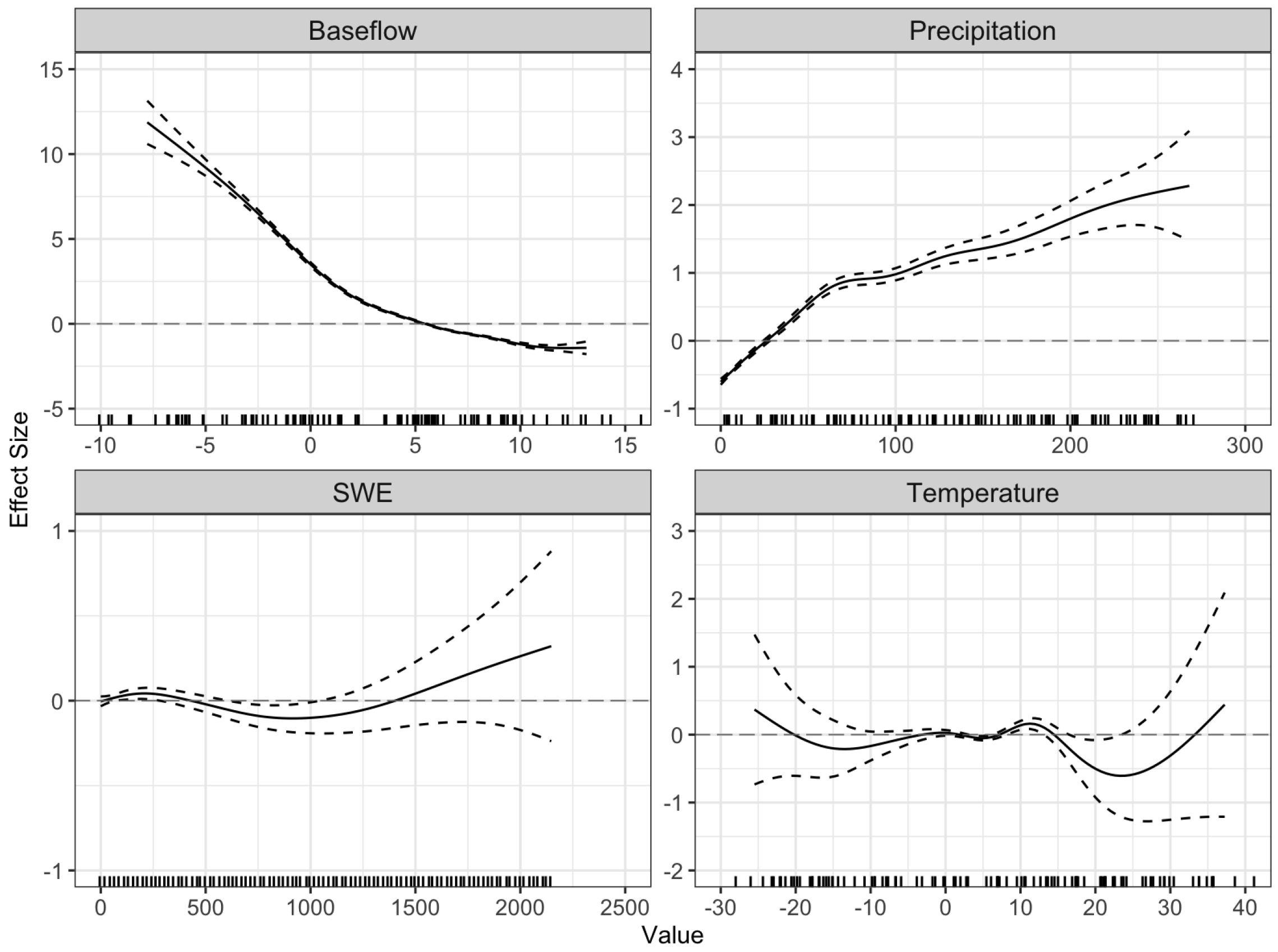
Starting with the GAM including SD, we see from Figure 7 that the variable with the largest effect on predicted surge is baseflow. This is likely because baseflow is the denominator of surge (see Equation (1)), so higher values produce lower predictions. Precip is positively associated with predicted surge, though the effect size is small in comparison with baseflow. Temp produces its highest effect size between zero and ten degrees, trending up again as it approaches 40 °C. SWE does not appear to contribute much to the predictions relative to the other variables, though we must recall that ROS events are correlated with both Precip, and Temp (see Figure 1), making it difficult to isolate the SWE effect in the model.
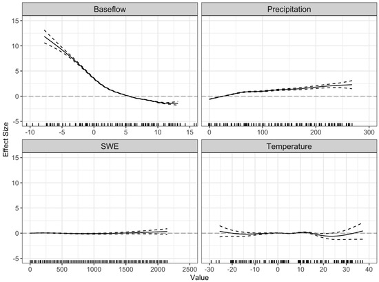
Figure 7.
Marginal effects of numeric variables included in the GAM without SD with fixed vertical axes. The solid line indicates the effect size, while the dashed line indicates 95 percent confidence intervals for each effect. The tick marks along the x-axis represent the values of the individual observations used to train the GAM.
Figure 8 is a repeat of Figure 7 that uses local scales for the vertical axis of each marginal effect to highlight trends that are not clearly visible in Figure 7. We see in Figure 8 that the relationship between SWE and predicted surge is non-linear, though the association does not appear to be significant based on the standard errors of the marginal effect. The model calculates a p-value of 0.015, indicating that the SWE effect is marginally significant.
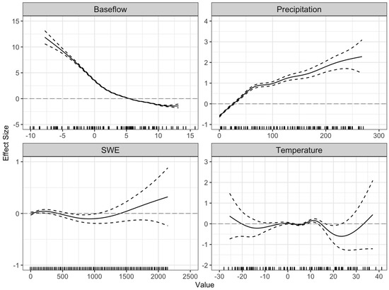
Figure 8.
Marginal effects of numeric variables included in the GAM without SD with varying vertical axes. The solid line indicates the effect size, while the dashed line indicates 95 percent confidence intervals for each effect. The tick marks along the x-axis represent the values of the individual observations used to train the GAM.
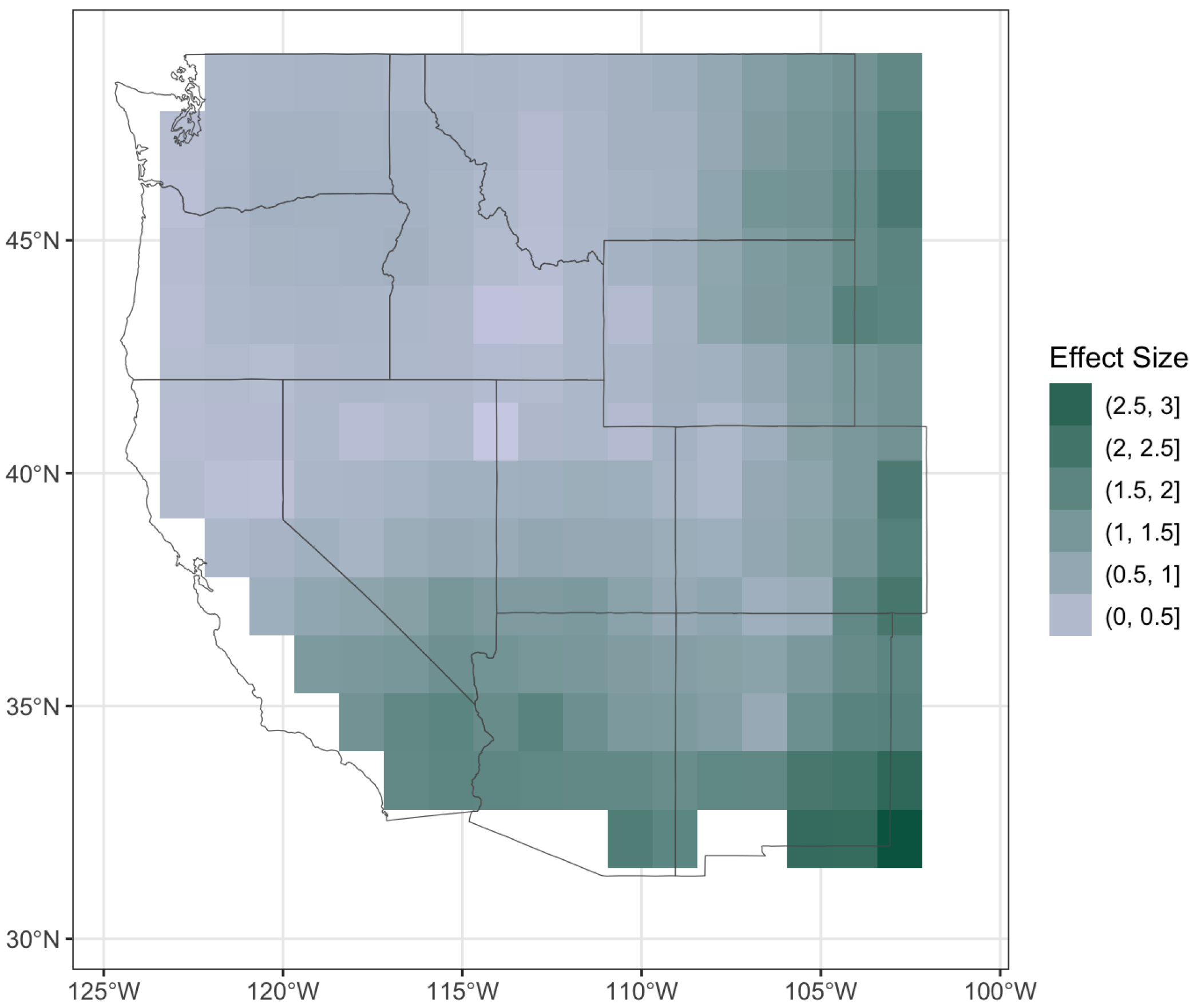
Figure 9 shows the marginal effect of the spatial term included in the GAM. It shows that, after accounting for the effects contributed by all other variables, the gages located in the southern and eastern parts of the region of interest tend to have slightly larger stream surges. We postulate that the purpose of this trend is to smooth out differences between areas with high and low water flows, but future work should investigate the reasons for these spatial patterns.
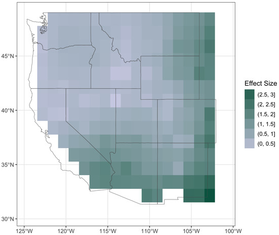
Figure 9.
Marginal effect of spatial term on the GAM excluding SD. Color represent the effect size for a given geographical location, with the legend split by equally spaced intervals.
3.4. Model Sensitivity
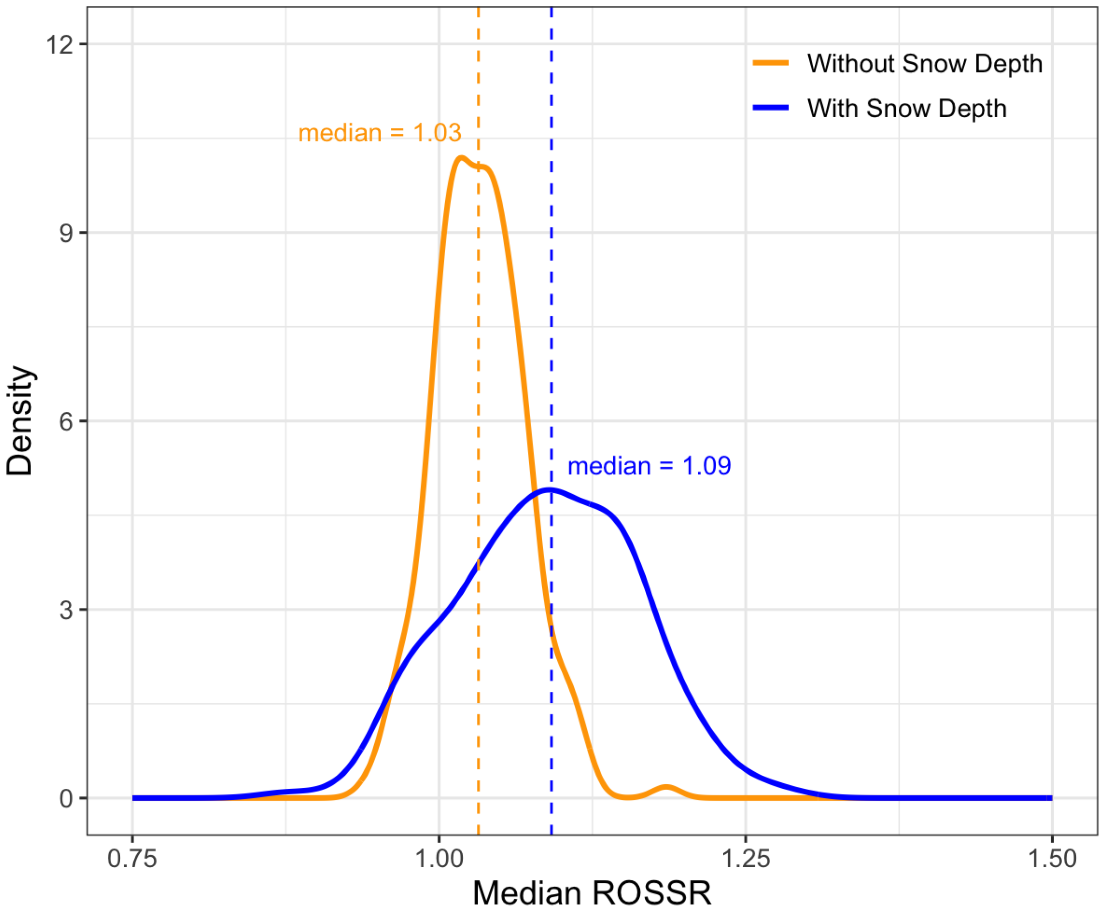
Recall that Figure 6 showed the distribution of ROSSR predictions from the GAMs across all streamgages. In this subsection, we use bootstrapping techniques to investigate the sensitivity of the median ROSSRs shown in Figure 6. As a brief summary, bootstrapping is a technique where the original dataset is sampled with replacement to create a “new” dataset of identical size. The new dataset includes repeats of some observations and omits other observations and provides a way to explore the sensitivity of estimations to perturbations in the input data. In this case, we generate predictions for 200 bootstrap samples and use them to approximate the distribution of the median r from each sample. The distributions of these medians are shown in Figure 10 for both GAMs. We observe that the model containing SD has notably more sensitivity/variability in the median ROSSR than the model excluding it. There is little visual evidence to suggest that the medians of either of these distributions are much different from 1.0, though the empirical results suggest that the values do tend to be higher (by 3–9 percent) when the SWE values are nonzero.
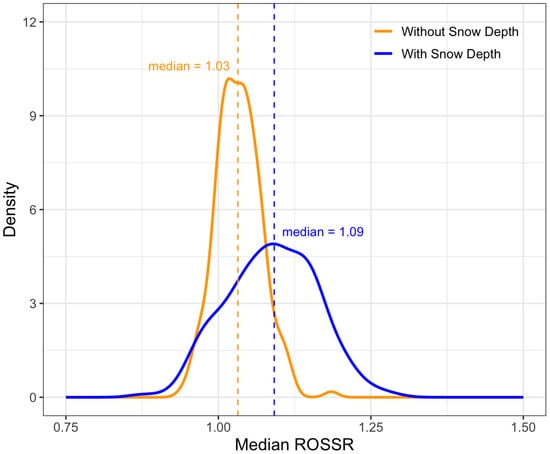
Figure 10.
Distribution of bootstrapped median ROSSR for both the GAM with SD and the GAM without.
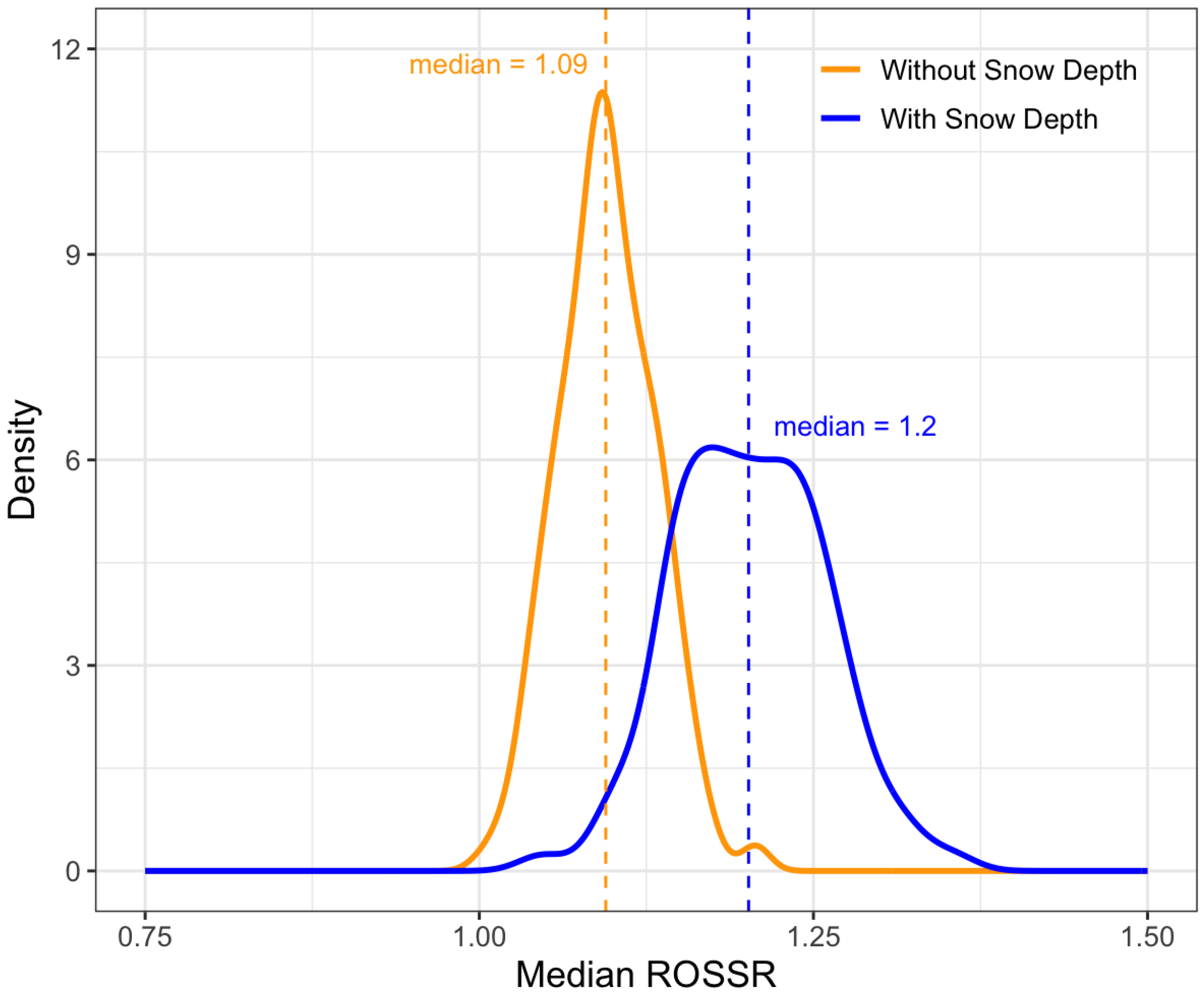
To further explore the sensitivity of the GAM projections to changes in ROS, Figure 11 also includes curves showing the ROSSR if the quantity for SD and SWE in the characteristic profiles were cut in half (for both the models including and excluding SD). Medians for both distributions increase substantially and variability decreases. There is strong visual evidence that the medians of both distributions are significantly above 1.0 after halving the snow accumulation profile. With these smaller SWE values, the models predict that surges will be 9–20 percent larger for an ROS characteristic profile as opposed to a non-ROS characteristic profile.
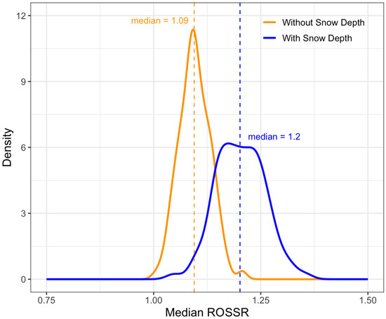
Figure 11.
Distribution of bootstrapped median ROSSR for both the GAM with SD and the GAM without, where the SWE and SD values from the characteristic profiles for ROS are cut in half.
The results from Figure 10 and Figure 11 suggest that the true median ROSSR lies in the interval between 1.03 and 1.2. Recall that the ROSSR represents a ratio between the ROS-typical surge and the non-ROS-typical surge as predicted by the GAM. This means that ratios above one indicate that the predicted stream surge for an ROS typical event is larger than the correpsonding prediction for a non-ROS event. In this case, the ratio indicates that ROS surges tend to be somewhere between 1.03 and 1.2 times, or equivalently 3–20 percent, larger than non-ROS surges in our region of interest. Keep in mind, however, that both ROS and non-ROS stream surges tend to occur with snow on the ground. The implications of using no snow in the non-ROS profile may overstate the influence of ROS on the model results. Future work needs to further the non-ROS profile construction to determine potential variations on the ROSSR results presented in this paper.
3.5. ML Application with Stressor
To compare the accuracy of ML approaches to predicting log-surge as compared to the GAMs, we use the ML model implementation available in the stressor R package [35]. We examine results from using the same subset of variables as the GAM containing SD, both including and excluding the latitude (lat) and longitude (lon) terms, as well as from including all summary statistics from variables shown in Table 1 besides SM measurements.
Table 8 shows the accuracy metrics for the top 5 (of 17) ML and linear regression models using the same 10-fold CV groupings at the streamgage level described previously. For most modeling methods, the formula including the lat/lon terms performed either the same or considerably better than the formula with no lat/lon. In addition to this, we observe that the highest performing model—the Extra Trees regressor containing just the GAM variables in addition to lat/lon—achieves a MSE 0.2 smaller than the MSE reported by the GAM model containing SD described previously. Only seven of the models applied using stressor perform better than the GAM with SD, and only four perform better than the GAM without. This suggests that our GAM models are competitive with other ML methods for modeling representations of stream surges from our dataset.
Table 8.
Cross validated results for the top five ML methods applied using the stressor R package. Errors colored red are smaller than the MSE of 0.93 reported by the GAM containing SD. ‘MSE’ columns represent ML models that use all candidate explanatory variables, while ‘GMSE’ columns only contain the subset of variables used in the final GAM formula from Equation (4). ‘+Geo’ indicates that the model includes lat/lon terms, while ‘−Geo’ indicates it does not. Model acronyms include Gradient Boosting (GB).
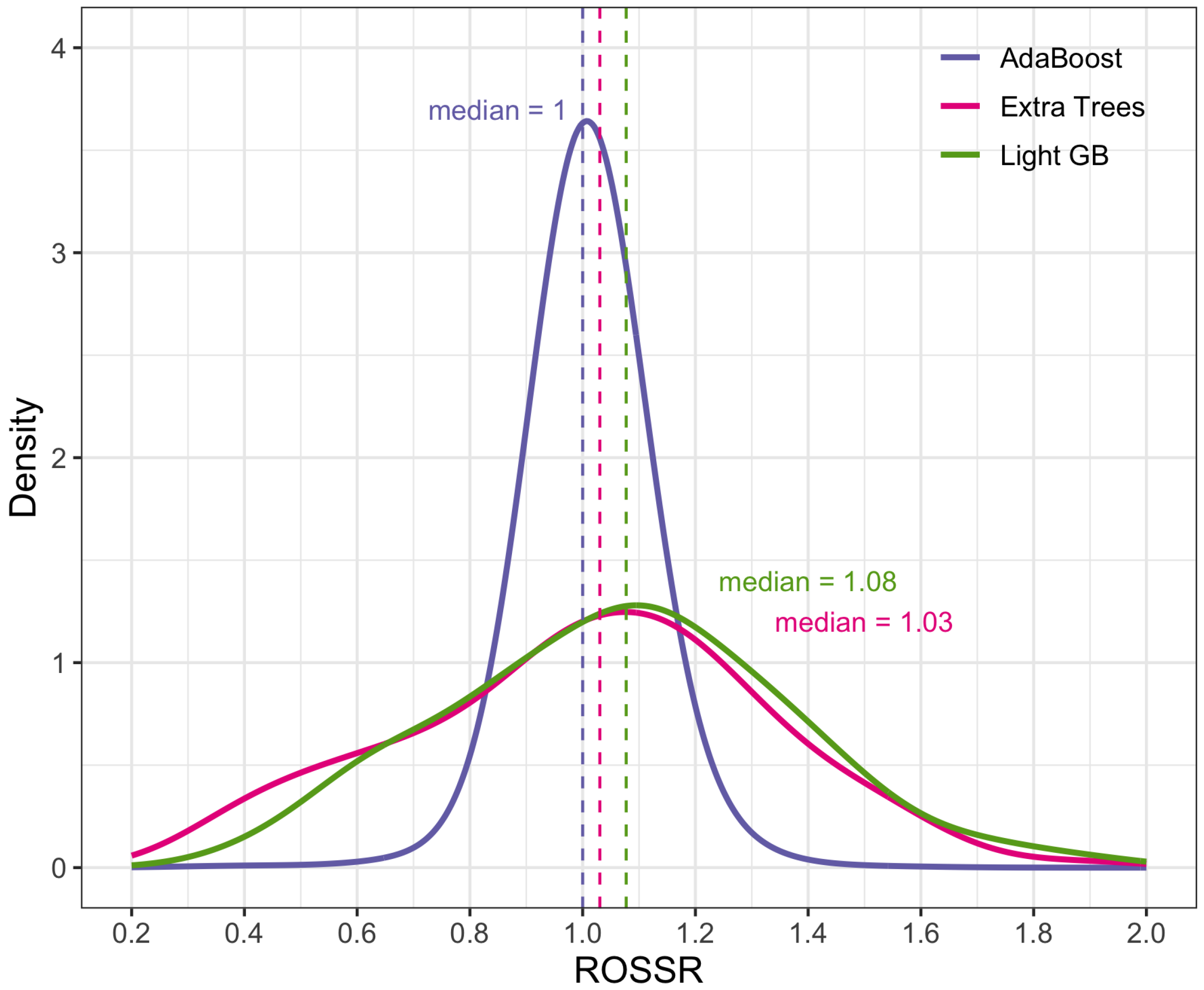
Using the subset of variables from the GAM (including lat/lon) and the non-ROS profiles with larger SWE, we plot the ROSSR distributions (no bootstrap) for the highest performing models across the board from Table 8—Light GB, Extra Trees, and AdaBoost—in Figure 12. The medians of all three distributions fall either close to or within the range of medians found from bootstrapping in Section 3.3. The Extra Trees and Light GB distributions have considerably more variability than the AdaBoost distribution. The AdaBoost distribution closely resembles the ROSSR distribution for the GAM excluding SD in Figure 10, while the Extra Trees and Light GB distributions follow a trend more similar to that of the GAM including SD. These ML results are in agreement with what we obtained with our GAMs, reinforcing the use of the GAM models as an effective method for modeling stream surge.
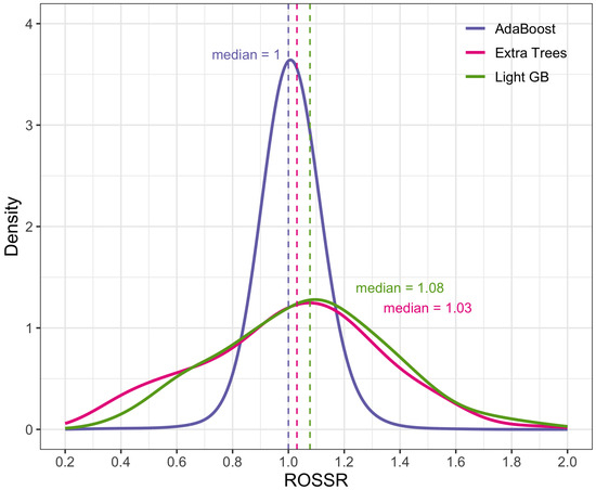
Figure 12.
Distributions of ROSSR for top three performing ML models from Table 8.
4. Conclusions
This paper presented a novel approach to quantifying the impact of ROS events on surges in streamflow relative to non-ROS-induced stream surges. This process required the development of a data workflow that automatically identified surges in streamflow and paired them to the snowpack, temperature, and precipitation conditions preceding the surge at nearby SNOTEL stations. The creation of this dataset allowed us to model the direct impacts of ROS weather events on streamflow response using GAMs and ML models, which suggested that ROS-induced stream surges tend to be 3–20 percent larger than non-ROS-induced stream surges.
One potential area of future work includes researching alternative methods to those used in this study for imputing flood stage thresholds not reported by the USGS. Additionally, we hypothesized an explanation for the marginal effects shown for the spatial terms in our GAMs in Figure 9, but a more in-depth investigation should examine more precise reasoning behind these spatial patterns. Further, the construction of non-ROS streamgage profiles should be further developed to determine potential variations on ROSSR results. Another area for future work, as mentioned previously in this paper, would be to replace SNOTEL measurements with gridded snow data such as SNODAS [30]. This would allow the analysis to be expanded to include non-mountainous regions. Additionally, future work should consider the impacts of vegetation and landscape characteristics on streamflow response to ROS events by incorporating data sources that provide that information.
Despite these opportunities for improvement, the adjustment factor we propose based on the dataset we created has the potential to benefit hydrologic design. For example, engineers can use our unitless flow adjustment factors (e.g., 1.03–1.2) to conservatively adjust design flow calculations in areas where ROS is expected to be an issue within the geographical limits of our study area, which is the western Continental United States. Additionally, the dataset and software described in this paper, made freely available online, facilitate exploration of the relationship between ROS events and streamflow data in areas outside of our study area.
Author Contributions
Conceptualization, B.L.B.; methodology, B.L.B.; software, E.W.; validation, E.W.; formal analysis, E.W.; investigation, E.W.; resources, B.L.B.; data curation, E.W.; writing—original draft preparation, E.W.; writing—review and editing, B.L.B.; visualization, E.W.; supervision, B.L.B.; project administration, B.L.B.; funding acquisition, B.L.B. All authors have read and agreed to the published version of the manuscript.
Funding
This research was funded in part by the Nevada Department of Transportation. The APC was covered in part by Utah State University’s Open Access Funding Initiative.
Data Availability Statement
The data and code supporting the results described in this paper are available in a publicly available repository (see [36]).
Acknowledgments
This manuscript was based upon results presented in Emma Watts’ Masters Thesis. We thank Jürgen Symanzik and Briana Bowen for their feedback on that thesis, which improved the quality of this manuscript. The authors also thank Kelvyn Bladen for his refinements to the rsnodas data download scripts, which were further adapted and refined in this paper. Lastly, the authors acknowledge the use of the R statistical software environment [37] along with the use of the following R packages: cardidates [26], cowplot [38], data.table [39], imputeTS [40], mgcv [41], rsnodas [21], sf [42], stressor [35], and tidyverse [43].
Conflicts of Interest
The authors declare no conflicts of interest. The funders had no role in the design of the study; in the collection, analyses, or interpretation of data; in the writing of the manuscript; or in the decision to publish the results.
Abbreviations
The following abbreviations are used in this manuscript:
| CV | Cross-Validation |
| GAM | Generalized Additive Model |
| HEC-HMS | Hydrologic Engineering Center Hydrologic Modeling System |
| HUC | Hydrologic Unit Code |
| MAE | Median Absolute Error |
| ML | Machine Learning |
| MSE | Mean Squared Error |
| NDOT | Nevada Department of Transportation |
| PRISM | Parameter-elevation Regressions on Independent Slopes Model |
| ROS | Rain-on-Snow |
| ROSSR | Rain-on-Snow Stream Surge Ratio |
| SD | Snow Depth |
| SM | Soil Moisture |
| SNOTEL | Snowpack Telemetry |
| SNODAS | Snow Data Assimilation System |
| SWE | Snow Water Equivalent |
| USGS | United States Geological Survey |
| WBD | Watershed Boundary Dataset |
References
- Berris, S.N.; Harr, R.D. Comparative snow accumulation and melt during rainfall in forested and clear-cut plots in the Western Cascades of Oregon. Water Resour. Res. 1987, 23, 135–142. [Google Scholar] [CrossRef]
- Musselman, K. Why Rain on Snow in the California Mountains Worries Scientists. The Conversation. 14 March 2023. Available online: https://theconversation.com/why-rain-on-snow-in-the-california-mountains-worries-scientists-201742 (accessed on 2 July 2024).
- Freudiger, D.; Kohn, I.; Stahl, K.; Weiler, M. Large-scale analysis of changing frequencies of rain-on-snow events with flood-generation potential. Hydrol. Earth Syst. Sci. 2014, 18, 2695–2709. [Google Scholar] [CrossRef]
- Beniston, M.; Stoffel, M. Rain-on-snow events, floods and climate change in the Alps: Events may increase with warming up to 4 °C and decrease thereafter. Sci. Total Environ. 2016, 571, 228–236. [Google Scholar] [CrossRef] [PubMed]
- Mazurkiewicz, A.B.; Callery, D.G.; McDonnell, J.J. Assessing the controls of the snow energy balance and water available for runoff in a rain-on-snow environment. J. Hydrol. 2008, 354, 1–14. [Google Scholar] [CrossRef]
- Musselman, K.N.; Lehner, F.; Ikeda, K.; Clark, M.P.; Prein, A.F.; Liu, C.; Barlage, M.; Rasmussen, R. Projected increases and shifts in rain-on-snow flood risk over western North America. Nat. Clim. Chang. 2018, 8, 808–812. [Google Scholar] [CrossRef]
- Yan, H.; Sun, N.; Wigmosta, M.; Skaggs, R.; Hou, Z.; Leung, R. Next-generation intensity-duration-frequency curves for hydrologic design in snow-dominated environments. Water Resour. Res. 2018, 54, 1093–1108. [Google Scholar] [CrossRef]
- Harpold, A.A.; Kaplan, M.L.; Klos, P.Z.; Link, T.; McNamara, J.P.; Rajagopal, S.; Schumer, R.; Steele, C.M. Rain or snow: Hydrologic processes, observations, prediction, and research needs. Hydrol. Earth Syst. Sci. 2017, 21, 1–22. [Google Scholar] [CrossRef]
- Wang, Y.H.; Broxton, P.; Fang, Y.; Behrangi, A.; Barlage, M.; Zeng, X.; Niu, G.Y. A Wet-Bulb Temperature-Based Rain-Snow Partitioning Scheme Improves Snowpack Prediction Over the Drier Western United States. Adv. Earth Space Sci. Geophys. Res. Lett. 2019, 46, 13825–13835. [Google Scholar] [CrossRef]
- Heggli, A.; Hatchett, B.; Schwartz, A.; Bardsley, T.; Hand, E. Toward snowpack runoff decision support. iScience 2022, 25, 104240. [Google Scholar] [CrossRef]
- Wayand, N.E.; Lundquist, J.D.; Clark, M.P. Modeling the influence of hypsometry, vegetation, and storm energy on snowmelt contributions to basins during rain-on-snow floods. Water Resour. Res. 2015, 51, 8551–8569. [Google Scholar] [CrossRef]
- Floyd, W.; Weiler, M. Measuring snow accumulation and ablation dynamics during rain-on-snow events: Innovative measurement techniques. Hydrol. Process. Int. J. 2008, 22, 4805–4812. [Google Scholar] [CrossRef]
- Würzer, S.; Jonas, T.; Wever, N.; Lehning, M. Influence of initial snowpack properties on runoff formation during rain-on-snow events. J. Hydrometeorol. 2016, 17, 1801–1815. [Google Scholar] [CrossRef]
- Wever, N.; Jonas, T.; Fierz, C.; Lehning, M. Model simulations of the modulating effect of the snow cover in a rain-on-snow event. Hydrol. Earth Syst. Sci. 2014, 18, 4657–4669. [Google Scholar] [CrossRef]
- Singh, P.; Spitzbart, G.; Hübl, H.; Weinmeister, H. Hydrological response of snowpack under rain-on-snow events: A field study. J. Hydrol. 1997, 202, 1–20. [Google Scholar] [CrossRef]
- Rücker, A.; Boss, S.; Kirchner, J.W.; von Freyberg, J. Monitoring snowpack outflow volumes and their isotopic composition to better understand streamflow generation during rain-on-snow events. Hydrol. Earth Syst. Sci. 2019, 23, 2983–3005. [Google Scholar] [CrossRef]
- Surfleet, C.G.; Tullos, D. Variability in effect of climate change on rain-on-snow peak flow events in a temperate climate. J. Hydrol. 2013, 479, 24–34. [Google Scholar] [CrossRef]
- Myers, D.T.; Ficklin, D.L.; Robeson, S.M. Hydrologic implications of projected changes in rain-on-snow melt for Great Lakes Basin watersheds. Hydrol. Earth Syst. Sci. 2023, 27, 1755–1770. [Google Scholar] [CrossRef]
- USACE. HEC-HMS. US Army Corps of Engineers. 2024. Available online: https://www.hec.usace.army.mil/software/hec-hms/ (accessed on 2 July 2024).
- USACE. What Is HEC-HMS and What Is Its Role? Hydrologic Engineering Center|US Army Corps of Engineers. 2024. Available online: https://www.hec.usace.army.mil/confluence/hmsdocs/hmsag/introduction/what-is-hec-hms-and-what-is-its-role (accessed on 2 July 2024).
- Schneider, L. rsnodas. 2023. Available online: https://github.com/lschneider93/rsnodas (accessed on 2 July 2024).
- USGS. USGS Water Data for the Nation, 2023. Available online: https://waterdata.usgs.gov/nwis (accessed on 2 July 2024).
- NWCC. Report Generator: Air & Water Database Report Generator. National Water and Climate Center|Natural Resources Conservation Service. 2024; Report Generator Version 2.0. Available online: https://wcc.sc.egov.usda.gov/reportGenerator/ (accessed on 2 July 2024).
- USGS. The National Map Downloader. U.S. Geological Survey. 2024. Available online: https://apps.nationalmap.gov/downloader/ (accessed on 2 July 2024).
- NACSE. PRISM Climate Data. Northwest Alliance for Computational Science and Engineering|Oregon State University. 2024. Available online: https://prism.oregonstate.edu/ (accessed on 2 July 2024).
- Rolinski, S.; Horn, H.; Petzoldt, T.; Paul, L. Identifying cardinal dates in phytoplankton time series to enable the analysis of long-term trends. Oecologia 2007, 153, 997–1008. [Google Scholar] [CrossRef]
- USGS. Sometimes the USGS Real-Time Stage Data Seems Too High (or Too Low). Are the USGS Data Inaccurate? U.S. Geological Survey. 2024. Available online: https://www.usgs.gov/faqs/sometimes-usgs-real-time-stage-data-seems-too-high-or-too-low-are-usgs-data-inaccurate (accessed on 2 July 2024).
- USGS. USGS Working to Restore Streamgages. U.S. Geological Survey. 2018. Available online: https://www.usgs.gov/news/featured-story/usgs-working-restore-streamgages (accessed on 2 July 2024).
- USDA. Snow Water Equivalent (SWE)—Its Importance in the Northwest. U.S. Department of Agriculture. 2024. Available online: https://www.climatehubs.usda.gov/hubs/northwest/topic/snow-water-equivalent-swe-its-importance-northwest (accessed on 2 July 2024).
- NSIDC. Snow Data Assimilation System (SNODAS) Data Products at NSIDC, Version 1; National Snow and Ice Data Center: Boulder, CO, USA, 2024; Available online: https://nsidc.org/data/g02158/versions/1 (accessed on 2 July 2024).
- Seaber, P.R.; Kapanos, F.P.; Knapp, G.L. Hydrologic Unit Maps. 1987. Available online: https://pubs.usgs.gov/wsp/wsp2294/ (accessed on 2 October 2024).
- Hastie, T.; Tibshirani, R.; Friedman, J. The Elements of Statistical Learning: Data Mining, Inference, and Prediction; Springer: Stanford, CA, USA, 2009. [Google Scholar]
- Wood, S.N. Thin plate regression splines. J. R. Stat. Soc. Ser. B Stat. Methodol. 2003, 65, 95–114. [Google Scholar] [CrossRef]
- Wendelberger, J.G. Smoothing Noisy Data with Multidimensional Splines and Generalized Cross-Validation; The University of Wisconsin-Madison: Madison, WI, USA, 1982. [Google Scholar]
- Haycock, S.; Bean, B. Stressor: Algorithms for Testing Models under Stress. 2024. R Package Version 0.1.0. Available online: https://cran.r-project.org/web/packages/stressor/index.html (accessed on 2 October 2024).
- Watts, E.; Bean, B. Supplementary Files for: Quantifying the Impact of Rain-On-Snow Induced Flooding in the Western United States. 2024. Available online: https://doi.org/10.26078/4bfb-87d9 (accessed on 2 October 2024).
- R Core Team. R: A Language and Environment for Statistical Computing; R Foundation for Statistical Computing: Vienna, Austria, 2023. [Google Scholar]
- Wilke, C.O. cowplot: Streamlined Plot Theme and Plot Annotations for ‘ggplot2’. 2024. R Package Version 1.1.3. Available online: https://CRAN.R-project.org/package=cowplot (accessed on 2 October 2024).
- Dowle, M.; Srinivasan, A. data.table: Extension of ‘data.frame’. 2023. R Package Version 1.14.8. Available online: https://CRAN.R-project.org/package=data.table (accessed on 2 July 2024).
- Moritz, S.; Bartz-Beielstein, T. imputeTS: Time Series Missing Value Imputation in R. R J. 2017, 9, 207–218. [Google Scholar] [CrossRef]
- Wood, S.N. Generalized Additive Models: An Introduction with R, 2nd ed.; Chapman and Hall/CRC: New York, NY, USA, 2017. [Google Scholar]
- Pebesma, E.; Bivand, R. Spatial Data Science: With Applications in R; Chapman and Hall/CRC: Boca Raton, FL, USA, 2023; p. 352. [Google Scholar]
- Wickham, H.; Averick, M.; Bryan, J.; Chang, W.; McGowan, L.D.; François, R.; Grolemund, G.; Hayes, A.; Henry, L.; Hester, J.; et al. Welcome to the tidyverse. J. Open Source Softw. 2019, 4, 1686. [Google Scholar] [CrossRef]


Disclaimer/Publisher’s Note: The statements, opinions and data contained in all publications are solely those of the individual author(s) and contributor(s) and not of MDPI and/or the editor(s). MDPI and/or the editor(s) disclaim responsibility for any injury to people or property resulting from any ideas, methods, instructions or products referred to in the content. |
© 2024 by the authors. Licensee MDPI, Basel, Switzerland. This article is an open access article distributed under the terms and conditions of the Creative Commons Attribution (CC BY) license (https://creativecommons.org/licenses/by/4.0/).