Article

Investigating a Century of Rainfall: The Impact of Elevation on Precipitation Changes (Northern Tuscany, Italy)

1
Department of Earth Science, University of Pisa, 56126 Pisa, Italy
2
Department of Agriculture, Food, Environment and Forestry, University of Florence, 50145 Firenze, Italy
3
Department of Civil and Industrial Engineering, University of Pisa, Largo Lucio Lazzarino, 56122 Pisa, Italy
4
Geosciences and Georesources Institute, National Research Council, 56124 Pisa, Italy
5
CIRSEC—Centre for Climate Change Impact, University of Pisa, Via del Borghetto 80, 56124 Pisa, Italy
*
Author to whom correspondence should be addressed.
Water 2024, 16(19), 2866; https://doi.org/10.3390/w16192866
Submission received: 28 August 2024 / Revised: 30 September 2024 / Accepted: 4 October 2024 / Published: 9 October 2024
(This article belongs to the Section Hydrology)

Abstract

:
Precipitation is crucial for water resource renewal, but climate change alters their frequency and amounts, challenging societies for correct and effective water management. However, modifications of precipitation dynamics appear to be not uniformly distributed, both in space and time. Even in relatively small areas, precipitation shows the coexistence of positive and negative trends. Local topography seems to be a strong driver of precipitation changes. Understanding precipitation changes and their relationship with local topography is crucial for society’s resilience. Taking advantage of a dense and long-lasting (1920–2019) meteorological monitoring network, we analyzed the precipitation changes over the last century in a sensitive and strategic area in the Mediterranean hotspot. The study area corresponds to northern Tuscany (Italy), where its topography comprises mountain ridges and coastal and river plains. Forty-eight rain gauges were selected with continuous annual precipitation time series. These were analyzed for trends and differences in mean annual precipitation between the stable period of 1921–1970 and the last 30-year 1990–2019. The relationship between precipitation changes and local topography was also examined. The results show the following highlights: (i) A general decrease in precipitation was found through the century, even if variability is marked. (ii) The mountain ridges show the largest decrease in mean annual precipitation. (iii) The precipitation change entity over the last century was not homogenous and was dependent on topography and geographical setting. (iv) A decrease in annual precipitation of up to 400 mm was found for the mountainous sites.

1. Introduction

Precipitation is one of the most fundamental climate processes, closely linked to water resource renewal, drought events, and floods, which deeply influence the resilience of society [1,2,3,4]. The impact of climate change on precipitation regimes and distribution also varies in space and time, enhancing the difficultiy of identifying and modelling changes in precipitation [5,6,7]. This research is confirmed by multiple studies analyzing changes in spatiotemporal precipitation patterns over recent decades around the globe [6,8,9,10,11,12]. When focusing on finer spatial resolution, precipitation changes show significant temporal and spatial variability, with positive and negative trends coexisting in relatively small areas [13,14,15,16]. These changes appear to be influenced by climate drivers like atmospheric circulation, local topography, and anthropogenic forcing [16,17,18,19]. At local scales and particularly in mountainous regions, topography imposes its signature on broader precipitation changes [19,20,21,22]. The description and analysis of the temporal and spatial patterns and variations in precipitation are thus fundamental for understanding the precipitation dynamics and drivers, the evaluation of climate models, and the quantification of the impacts of changes in precipitation on water resources [1,8,14,18]. In this context, long-term and spatially dense precipitation monitoring networks are fundamental.
In this work, we take advantage of a dense rain gauge network, which has been active since the beginning of the 1920s in northern Tuscany (Italy). The area is topographically complex with mountain ridges and coastal and river flood plains. The proximity to the Mediterranean basin strongly affects the precipitation dynamics, with the annual precipitation values being among the highest in Italy and Europe.
Located in the Mediterranean basin and characterized by mountain ridges, northern Tuscany can be considered a climate change hotspot [19,23,24,25]. Several studies have already indicated a potential overall decline in precipitation in the region since the 1950s, underscoring its vulnerability to climate change [18,26,27].
All these characteristics, make this area optimal for studying precipitation variability, in time and space. Thus, the main objectives of the present work are the following:
o
evaluation of the changes in annual precipitation and their spatial patterns in the study area over the last century;
o
analysis of how topography can influence precipitation changes at the local scale.
Additionally, northern Tuscany hosts some of the most relevant water resources of the entire region, thus enhancing the social value of such an analysis [28,29].

2. Study Area

The study area corresponds to northern Tuscany and includes the Livorno–Pisa–Lucca–Pistoia plain to the south and the Apuan Alps and northern Apennine to the north (Figure 1).
The landscape is particularly varied, presenting flat and hilly areas in the southern portion and steep mountains in the northern one, where the altitude reaches 2000 m above sea level. The climate is consequently variable, although predominantly of Mediterranean type with hot, dry summers and mild, wet winters [30,31,32]. The mean annual precipitation varies from 900–1000 mm in the southern flat-hilly area to more than 2000 mm in the mountainous northern one, with a maximum of rainfall in autumn and a minimum in summer [33,34,35,36,37]. The precipitation regime is mainly conditioned by eastward-moving atmospheric disturbances originating over the Atlantic Ocean, by perturbations coming from the Scandinavian and Siberian regions, and by convective storm events originating over the Mediterranean area and Genoa Gulph [31,38]. The Apuan Alps and northern Apennine represent the main regional reliefs, acting as a barrier for the humid air masses from the Mediterranean Sea and the Atlantic Ocean [31,38]. The bi-directional W-SW and NE-E origin of the atmospheric disturbances are highlighted by the corresponding dominant wind direction registered along the ridges of the northern Apennine [39,40]. Due to the interaction between atmospheric perturbations and the Apuan Alps’ steep landscape, the average annual rainfall of 3000 mm is reached and sometimes exceeded [18,35,36,41,42]. Both for the whole of Tuscany and its northern portion, a general decreasing trend in precipitation has been recognized [26,27].
Moreover, the study area often experienced extreme meteorological events, also inducing heavy damage and deaths [36,43,44].

3. Materials and Methods

Daily rainfall data of 49 rain gauges were acquired from the open database of the Tuscany Region Hydrologic Service [39] (Figure 1). Precipitation records covered the period from 1921 to 2019. The high number of rain gauges and the extent of the study area offer a dense monitoring network, resulting in a particularly rich and long dataset.

3.1. Deriving and Checking Annual Precipitation Series

Annual precipitation series were obtained from the daily rainfall data for each rain gauge. When necessary, the filling of missing yearly data was carried out via linear regression with nearby rain gauges [45,46]. Given a rain gauge with missing annual precipitation data, a rain gauge sharing a similar physiographical context, closer than 10 km, and with a coefficient of determination R2 ≥ 0.8 (with a linear regression model) was identified. The missing data of the receiving rain gauge were then derived by linearly interpolating the donor rain gauge annual precipitation data. The annual precipitation series were tested for homogeneity with the double mass curve of cumulative annual precipitation versus time in years [47]. Two rain gauges of the dataset presented an anomalous change in their records and, therefore, were discarded. The 47 remaining rain gauges did not present abrupt changes in the double mass curve, suggesting stability in measuring conditions.

3.2. Precipitation Interpolation

Since an updated and validated map of the mean annual precipitation (MAP) is still missing for the studied area, an interpolation is provided here. The MAP value for each rain gauge was computed for the years 1990–2019 and interpolated by universal kriging, with elevation as an external variable. The interpolation procedure, performed by the “autoKrige” function of the “automap” package in R language [48,49], was chosen to obtain the spatial distribution of the 1990–2019 MAP. The interpolation was performed on a sampling grid of 100 × 100 m spaced points. All the geographical data are reported in the EPSG:3003 coordinate system. The elevation value for each interpolated point was derived from the regional DTM of Tuscany, provided by the Tuscany Region Cartography website (https://www502.regione.toscana.it/geoscopio/cartoteca.html accessed on 3 March 2019). To validate the interpolation, a leave-one-out cross-validation was performed for all the considered rain gauges [50,51]. The map of MAP for the 1990–2019 period was then used as a reference in the following evaluations.

3.3. Analysis of Annual Precipitation Variation

Annual precipitation variations over an entire century were most likely not linear, and thus their description with a single linear model may be incorrect, even in the case of a trend detected with a p-value < 0.05. Two strategies were adopted to analyze changes and fluctuations in annual precipitation. Firstly, an analysis of the annual precipitation changes and a discrimination of stationary and changing periods were performed at a regional scale. Then, the MAPs were compared and statistically tested between trend-free periods. Indeed, if a significant trend affects a data series, using the mean value to represent that data would at least lead to a loss of information and an incorrect representation of the process.

3.3.1. Trend Analysis

The analysis and description of annual precipitation fluctuations over the last century at a regional scale were conducted as follows. For each rain gauge dataset, the Mann–Kendall non-parametric trend detection test was executed on a 30-year moving window. The thirty-year length was adopted since it is globally recognized as the minimum length for climate characterization [52]. The Mann–Kendall test was applied, being widely used in hydrological and climatological time series analyses for the detection of trends [53,54,55,56]. The test was performed using the rtk function of the R rkt package [48,57]. A brief description of the test is provided here [54,55]. Let X1, X2, …, Xn be a sequence of n observations ordered in time. The Mann–Kendall test statistic S is defined as
S = i = 1 n 1   j = i + 1 n s g n X j X i
with
s g n x = + 1   i f   x > 0   0   i f   x = 0 1   i f   x < 0
The S statistic sign indicates the direction of the data variation. The standardized test statistic Z is computed by
Z =   S 1 V a r ( S )   if   x > 0   0   if   S = 0 S + 1 V a r ( S )   if   x < 0
The p-value of the Mann–Kendall statistic (S) can be estimated using the normal cumulative distribution function ( Φ ) :
p = 0.5 Φ ( Z ) ,   with   Φ Z = 1 2 π 0 Z e t 2 / 2 d t
The average S value of all the rain gauges was calculated for each of the 30-year time windows and plotted with the count of p-values < 0.05, identifying the presence of significant trends. It was then possible to define sub-periods where changes in annual precipitation occurred as compared to the stationary periods.

3.3.2. Differences in Mean Annual Precipitations

To evaluate changes in annual precipitation over the last century, the most recent thirty-year period (1990–2019) MAP was compared with the previous stationary periods. Differences in MAP were tested by the t-test for all the rain gauges. The t-test was computed with the “t-test” function of the R stats package [48,58]. Before performing the t-test, the two compared periods were tested for Gaussian population distribution and absence of a trend. These are the assumptions for the validity of the t-test. The Gaussian distribution test was performed with the Shapiro.test function of the R stats package. Trend testing was accomplished by the Mann–Kendall test with the rtk function mentioned before [48]. In the case of non-Gaussian data, the MAP differences were recalculated with a bootstrap procedure computed with the boot function of the boot package [48,59].
The differences in MAP and the associated t-test statistics were used to evaluate the variation in precipitation between the considered periods. The confidence intervals of the differences in MAP were obtained by computing their standard deviations [58]:
σ D x y = V A R ( P x ) N A P x + V A R ( P y ) N A P y
where
  • σ D x y —standard deviation of the difference in MAP between the periods x and y.
  • V A R ( P x / y ) —variance in the annual precipitation values in the period x or y.
  • N A P x / y —number of observations in the x or y period.
The differences in MAP and the associated t-test p-values were plotted over the study area for geographical evaluation.

3.4. Morphological and Geographical Influence on the Annual Precipitation Changes

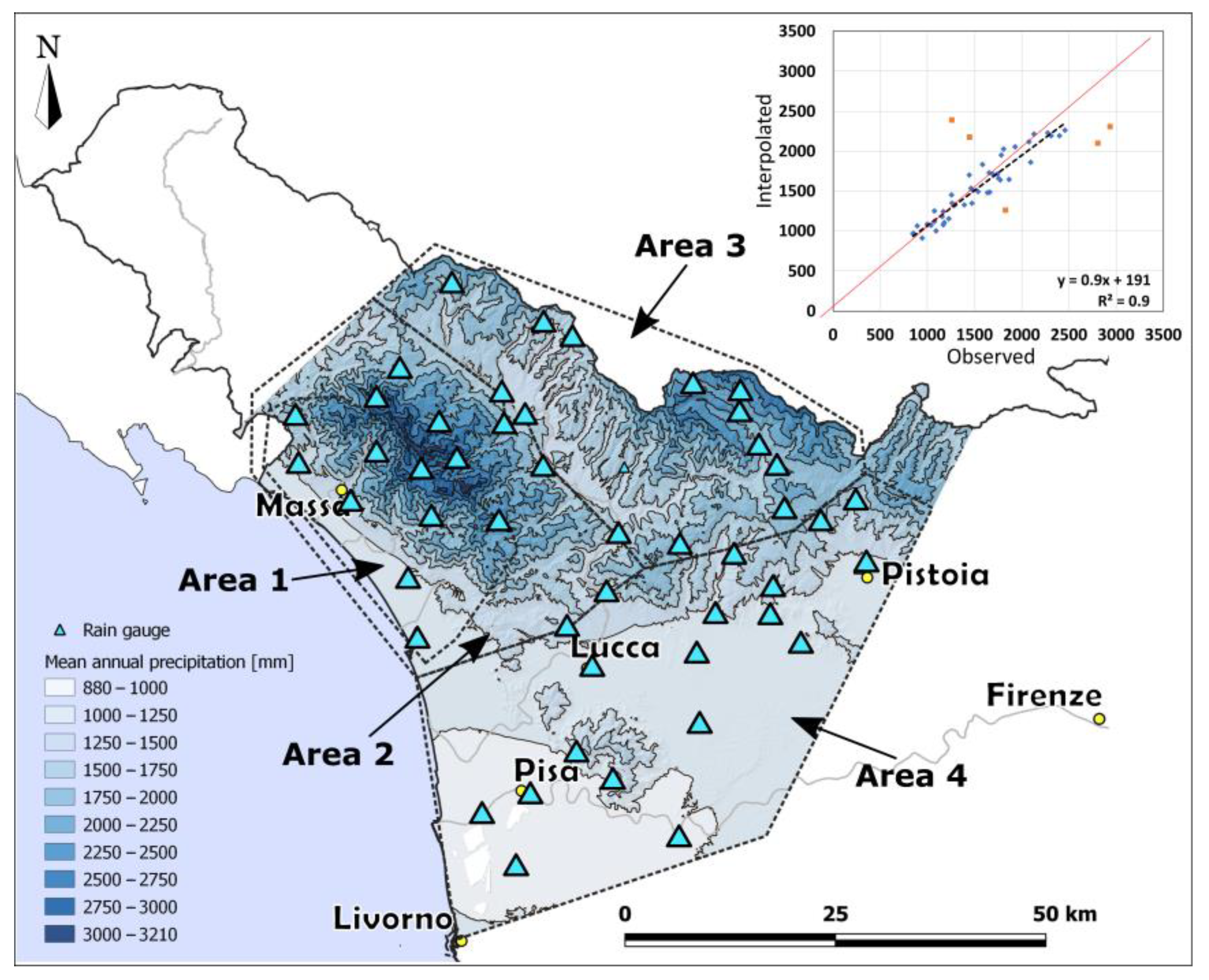
Within the study area, four different sub-areas were identified based on their morphological features and geographic locations (Figure 2). Area 1 includes the western side (seaside) of the Apuan Alps; Area 2 includes the entire Apuan Alps’ mountain belt, which is exposed to the sea influence; Area 3 includes the northern Apennine, more exposed to both western and eastern atmospheric perturbations; and Area 4 comprises the southern plain areas extending from the seaside between Pisa and Livorno toward the E-NE. The differences in MAP were grouped according to these four sub-areas. The dependency on local morphology and particularly the correlation with elevation were evaluated. The lmfunction of the R stats package was used to derive the linear best fit of differences in MAP compared with the rain gauges elevation. The errors in the regression coefficient and intercept were calculated as described by [58] for the general case of data with different uncertainties.

4. Results

The MAP of the 1990–2019 period was obtained (Figure 2). Excluding five outliers, the interpolated vs. observed linear regression shows a slope of 0.9 and R2 of 0.9, proving the goodness of the interpolation. The map (available from [60]) shows that the MAP of the study area in the 1990–2019 period ranges from a minimum of 887 mm to a maximum of 3210 mm, with a mean of 1498 mm. As expected, the larger values of MAP are mainly found in the Apuan Alps, and secondarily in the northern Apennine. The southern plain area is characterized by lower MAP values.

4.1. Annual Precipitation Fluctuations

The results of the Mann–Kendall test on the 30-year time windows in the study period (1921–2019) are shown in Figure 3. In the first half of the analyzed period (ca., 1921–1970), the average S of all rain gauges fluctuate between positive and negative values, with very few rain gauges possessing a p-value lower than 0.05. This period is therefore considered not affected by significant trends in precipitation. Between the beginning of the 1970s and 1994, the average S parameter remained at negative values, joined with an increase in the number of rain gauges possessing a p-value lower than 0.05. This major decrease is shown throughout the study area as displayed by the heatmap of Figure 4, more marked in the sub-periods of 1970–1980 and 1989–1993. After 1994, a general increase in the average S statistic is again detected along almost all the considered rain gauges, even though few rain gauges have a p-value lower than 0.05.

4.2. Annual Precipitation Differences

It appeared that 1921–1970 can be considered a stationary period for the annual precipitation. The datasets were split into two sub-periods each, 1921–1970 and 1990–2019, for a total of 94 sub-datasets. Differences in MAP between the 1990–2019 and the 1921–1970 periods were then computed and tested for significance, as described in the Section 3. Before computing the t-test for the significance of differences in the MAP, the normality and absence of trends in the comparison periods for each rain gauge were checked. Of the 94 tested sub-datasets, 7 (4 in the 1921–1970 period and 3 in the 1921–1990 period) were affected by significant trends (Mann–Kendall p-value < 0.05) and 10 (3 in the 1921–1970 period and 7 in the 1921–1990 period) were significantly non-Gaussian. Given the small number of datasets affected by trends, all of these were kept in the analysis of the differences to prevent loss of information.
For trend-affected datasets, the mean is, therefore, an average of a changing process over the observed period rather than the mean value of a stationary process. The standard deviations were computed after detrending the considered dataset. For the non-Gaussian datasets, from the Central Limit Theorem [61], we can assume that their distribution of means is normally distributed and, consequently, the t-test is still applicable using the sample standard deviation. However, the bootstrap testing was additionally performed to verify the goodness of the estimated differences in the means and relative standard deviations. The bootstrap MAP differences were almost equal to their first estimation. Also, standard deviations calculated by Equation [5] and the bootstrap procedure produced differences lower than 10–20%. Given the agreement with the bootstrap differences in MAP, the non-Gaussian datasets were also kept in the following evaluations.
Most rain gauges with significant MAP differences (p-value ≤ 0.05, 36% of the dataset) are located in the northeastern mountainous portion of the area, and the differences are mainly negative (Figure 4). The rain gauges with negative differences are larger in number (87% of all the rain gauges), with the following p-value divisions: p-value ≤ 0.05 is 32% of the total; 0.1 ≤ p-value < 0.05 is 19% of the total; and p-value > 0.1 is 36% of the total. These areas appear to have experienced a higher negative variation in MAP, up to −420 mm, between the 1990–2019 period and the stationary 1921–1970 period.
The map of Figure 4 shows that, in the study area, negative MAP differences are dominant. The positive MAP differences account for 13% of all the rain gauges, with the following p-value divisions: p-value ≤ 0.05 is 4% of the total and p-value > 0.1 is 9% of the total.
The coastal plain and the southeastern plain area show minor MAP positive differences and, in a few cases, negative. Consequently, these latter sub-zones seem less subject to a change in mean annual precipitation in the analyzed periods.

4.3. The Effect of Elevation

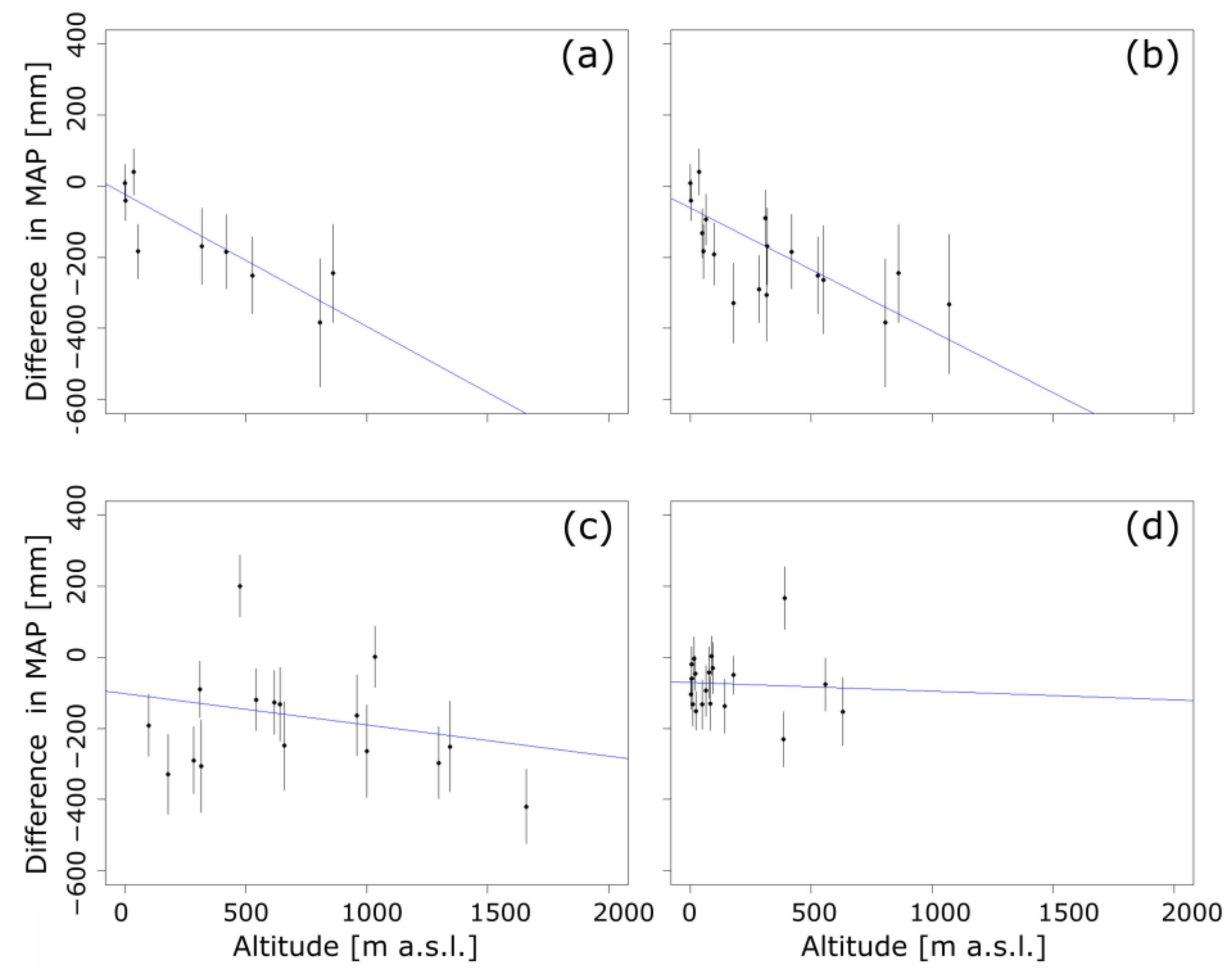
The correlation between the difference in MAP and elevation was evaluated for both periods 1921–1970 and 1990–2019. The rain gauges were divided into groups according to the four investigated sub-areas. Each rain gauge falling on the border of two sub-areas was included in both respective groups.
The four areas show a different distribution of differences in MAP when plotted against the altitude of the measuring location (Figure 5). Data from Areas 3 and 4 are scattered and show no significant linear correlation between MAP differences and elevation (Table 1). Data from Areas 1 and 2 appear to present a significant negative linear correlation between the mean annual precipitation difference and elevation, with a higher R2, coefficient p-values <0.05, and good χ2 (Figure 5 and Table 1). The regression coefficients are of similar amplitude between Area 1 and Area 2 (between −0.29 and −0.39 mm/m).

4.4. Interpolation of Differences in Precipitation

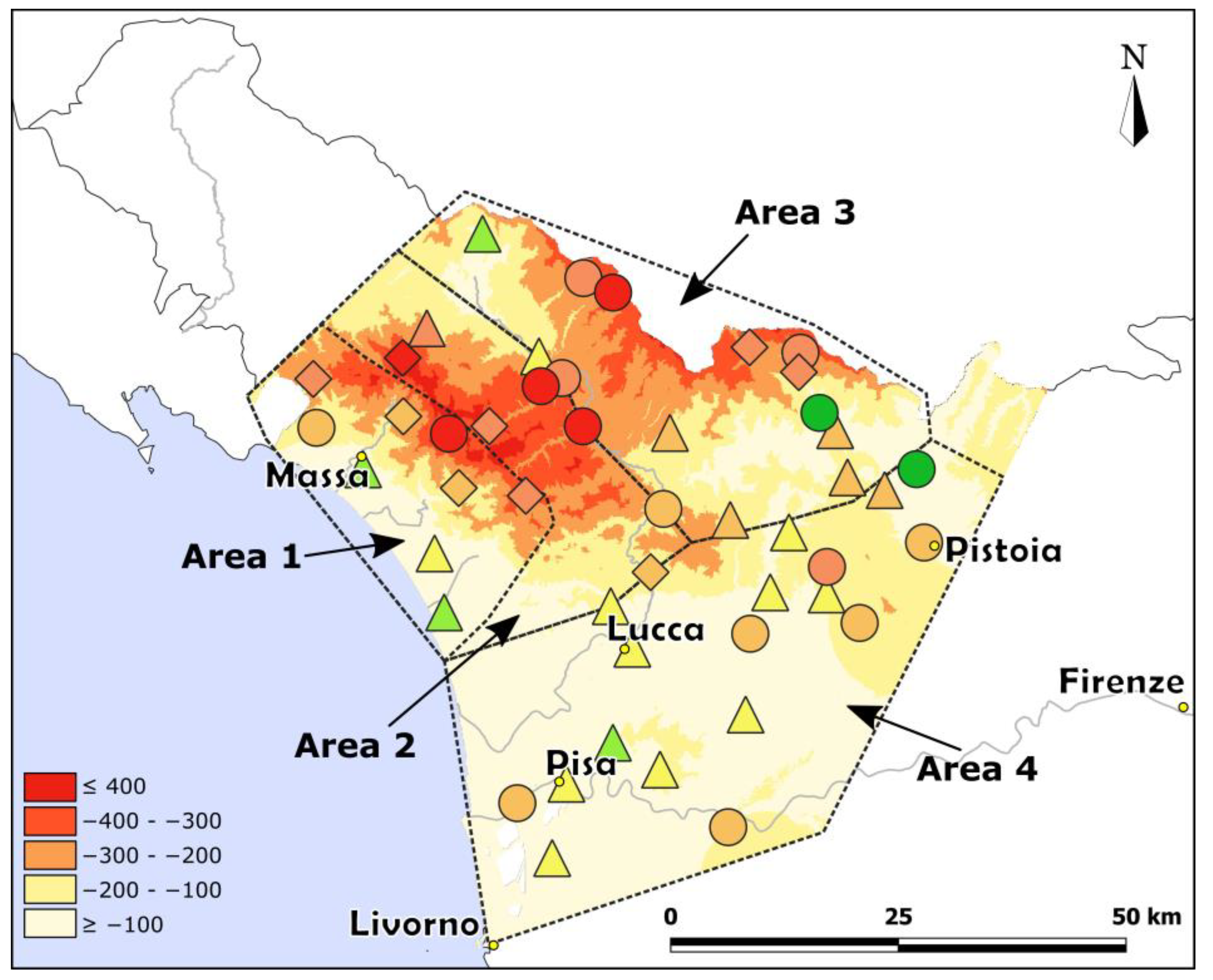
Given the paramount importance of the study area also for the regional water resources, an interpolation of the MAP reduction that occurred between the last 30-year period (1990–2019) and the more stationary 1921–1970 period was performed. The 1921–1970 MAP was interpolated by kriging with external drift, as described in the Section 3. Then, the two rasters of the interpolated MAP for the periods 1990–2019 and 1921–1970 were subtracted to obtain the spatial distribution of the differences in MAP (Figure 6). The southern plain and the coastal plain show the smallest changes in MAP, while the mountainous areas experienced a higher reduction in precipitation, with values exceeding 400 mm. The Apuan Alps (Area 2) show the highest differences in MAP, while on the northern Apennine ridge (Area 3) the differences in MAP are less pronounced, despite comparable elevations. This observation agrees with the identified relationship between differences in MAP and elevation for the Apuan Alps (Area 2).

5. Discussion

Both the Apuan Alps and the northern Apennine are characterized by higher MAP values in the study area for the most recent 1990–2019 period. This is undoubtedly related to the well-known orographic precipitation enhancement process [62,63,64,65]. Despite the similar and often higher altitude of the northern Apennine compared to the Apuan Alps, the latter are characterized by higher MAP values (maximum around 3200 mm), probably in relation to their proximity to the sea, which apports humid western air masses. Moreover, the northern Apennine is in the drier leeward [62] side of the Apuan Alps with respect to the humid western air masses.
The MAP fluctuations (Figure 3) are in agreement with the changes in precipitation identified by [18] from the 1950s onward. However, we extended the analyses backward by more than 30 years, showing the relative stability of the 1921–1970 period in the analyzed area. The analysis also points out that the period from 1960 to 1990, usually adopted as a climatic reference [52], does not have stable annual precipitation for the studied area and should be used with caution.
The analysis of the last century’s fluctuation in annual precipitation identified that significant and decreasing trends are mainly distributed in the mountainous parts of the study area. This result is in contrast with the work of [19], which found a decrease in precipitation in the low-land area of the Po plain and no significant changes in the Alpine region. However, these results are derived from a shorter period (1960–1990) in a different geographical setting.
As expressed by [62] and references therein, the orographic enhancement is influenced by multiple factors like cloud processes, interaction of the atmospheric flow with orography, and general atmospheric circulation. Therefore, given the analyzed dataset, it is not easy to argue the root causes of the larger decrease in precipitation at higher altitudes, which can be related to multiple reasons from changes in large-scale circulation patterns to changes in local factors (temperature gradients, condensation levels, hydrometeor formation, pre-perturbation conditions, etc.) [66,67,68].
The reduction in MAP showed a negative and significant correlation with elevation in the Apuan Alps (Areas 1 and 2, Figure 2 and Figure 3), in contrast with the other mountainous ridge (northern Apennine, Area 3, Figure 2 and Figure 3), where there is no such significant correlation. This diversity may be related to the different morphological and meteorological settings. Indeed, as underlined previously, the Apuan Alps are more influenced by the proximity to the sea and the consequent orographic perturbations, protecting the northern Apennine from these meteorological events. The reduction in wind speed and storminess in the Mediterranean area [2,69] and the consequent lower orographic enhancement may be the cause of such a negative correlation between precipitation and elevation in the Apuan Alps. On the other hand, larger and less orographically sensitive perturbations may cause similar amounts of precipitation in both the Apuan Alps (Area 2) and the northern Apennine (Area 3), not showing any relation with elevation. However, as well summarized by [31], the Mediterranean climate and its changes are markedly variable in space due to the morphological complexity of the area and to the dependency of different atmospheric circulations, and any analysis of changes in dominant perturbation dynamics has yet to be performed.
Aside from the actual causes, which need further investigation, the different correlation between MAP differences and elevations for the four investigated areas also points out the variability in precipitation changes at a local scale, similar to what was observed by other authors [14,16,70].
The derived interpolation of differences in MAP confirmed that the mountainous areas are more vulnerable to annual precipitation variations, inducing potentially serious consequences on strategic water resources management [28], which require an increased level of attention. Therefore, further investigation and particularly the continuation of the monitoring of precipitation are necessary for the efficient assessment, forecast, and management of water resources.

6. Conclusions

In this work, the mean annual precipitation in the last century (from 1921 to 2019) in northern Tuscany was analyzed thanks to a dense network of rain gauges. This study aimed to perform a spatially refined analysis of the possible changes in the annual precipitation over the study area and their correlation with local topography.
A map of the mean annual precipitation over the last thirty-years period (1990–2019) was constructed, filling the gap of an updated and validated precipitation interpolation in northern Tuscany.
The main results of this study are as follows:
Annual precipitation was approximately stable during the 1921–1970 period.
Changes in precipitation were mostly negative from the 1970s to the beginning of the 1990s and positive but less marked from the 1990s onwards.
The mountainous areas showed a greater reduction in annual precipitation up to −400 mm over the observation period.
Over the Apuan Alps—the mountain ridge closer to the sea—the decrease in precipitation is negatively correlated with altitude. This correlation is absent over the innermost mountain ridge (northern Apennines).
Further investigations are needed to properly assess the causes of such local differences in annual precipitation variation. Dense and long-lasting meteorological networks are of paramount importance for the accurate analysis of climatic variability and should be promoted and maintained in all countries to study, foresee, and model climatic changes with consequences on communities and ecosystems.

Author Contributions

Conceptualization, M.N. and M.B.; methodology—software, M.N. and M.B.; data curation, M.N.; validation, M.N., M.B., B.R. and R.G.; formal analysis, M.N. and M.B.; resources, R.G.; writing—original draft preparation, M.N.; writing—review and editing, M.N., M.B., B.R. and R.G.; visualization, M.N. and M.B.; supervision, M.B., B.R. and R.G.; project administration, R.G. All authors have read and agreed to the published version of the manuscript.

Funding

This research was funded by the Tuscany Region Por FES 2014/2020 funds (CUP_ I51J20000180002) and supported by the University of Pisa. This work was supported by the PRA 2022-23 Project “Variazioni di frequenza delle alluvioni dell’Arno negli ultimi 3000 anni e loro effetti” (CUP_I53C22001890001), promoted by the University of Pisa.

Data Availability Statement

Daily precipitation datasets were derived from the Open Regional Service of Tuscany [39]. All data comprising the annual precipitation time series, the rain gauge locations as shape files, and the derived raster map of the mean annual precipitation in the period from 1990 to 2019 and the differences in mean annual precipitation are available in [60].

Acknowledgments

The authors also want to acknowledge the Open Regional Service for territorial data for maintaining and providing good-quality and freely accessible datasets.

Conflicts of Interest

The authors declare no conflicts of interest.

References

  1. Dams, J.; Salvadore, E.; Van Daele, T.; Ntegeka, V.; Willems, P.; Batelaan, O. Spatio-Temporal Impact of Climate Change on the Groundwater System. Hydrol. Earth Syst. Sci. 2012, 16, 1517–1531. [Google Scholar] [CrossRef]
  2. IPCC. Climate Change 2022—Impacts, Adaptation and Vulnerability: Working Group II Contribution to the Sixth Assessment Report of the Intergovernmental Panel on Climate Change, 1st ed.; Cambridge University Press: Cambridge, MA, USA, 2023; ISBN 978-1-00-932584-4. [Google Scholar]
  3. Vörösmarty, C.J.; Green, P.; Salisbury, J.; Lammers, R.B. Global Water Resources: Vulnerability from Climate Change and Population Growth. Science 2000, 289, 284–288. [Google Scholar] [CrossRef] [PubMed]
  4. World Meteorological Organization. State of Global Water Resources Report. 2022 WMO-No. 1333; World Meteorological Organization (WMO): Geneva, Switzerland, 2023; p. 66. [Google Scholar]
  5. Bird, L.J.; Bodeker, G.E.; Clem, K.R. Sensitivity of Extreme Precipitation to Climate Change Inferred Using Artificial Intelligence Shows High Spatial Variability. Commun. Earth Environ. 2023, 4, 469. [Google Scholar] [CrossRef]
  6. IPCC. Climate Change 2007: The Physical Science Basis: Contribution of Working Group I to the Fourth Assessment Report of the Intergovernmental Panel on Climate Change; Solomon, S., Qin, D., Manning, M., Chen, Z., Marquis, M., Averyt, K.B., Tignor, M., Miller, H.L., Eds.; Intergovernmental Panel on Climate Change; Cambridge University Press: Cambridge, MA, USA, 2007; ISBN 978-0-521-88009-1. [Google Scholar]
  7. Kidd, C.; Huffman, G. Global Precipitation Measurement. Meteorol. Appl. 2011, 18, 334–353. [Google Scholar] [CrossRef]
  8. Adler, R.F.; Gu, G.; Sapiano, M.; Wang, J.-J.; Huffman, G.J. Global Precipitation: Means, Variations and Trends During the Satellite Era (1979–2014). Surv. Geophys. 2017, 38, 679–699. [Google Scholar] [CrossRef]
  9. Deitch, M.; Sapundjieff, M.; Feirer, S. Characterizing Precipitation Variability and Trends in the World’s Mediterranean-Climate Areas. Water 2017, 9, 259. [Google Scholar] [CrossRef]
  10. Easterling, D.R.; Arnold, J.R.; Knutson, T.; Kunkel, K.E.; LeGrande, A.N.; Leung, L.R.; Vose, R.S.; Waliser, D.E.; Wehner, M.F. Precipitation change in the United States. In Climate Science Special Report: Fourth National Climate Assessment, Volume I; Wuebbles, D.J., Fahey, D.W., Hibbard, K.A., Dokken, D.J., Stewart, B.C., Maycock, T.K., Eds.; U.S. Global Change Research Program: Washington, DC, USA, 2017; pp. 207–230. [Google Scholar] [CrossRef]
  11. Hu, Z.; Zhou, Q.; Chen, X.; Qian, C.; Wang, S.; Li, J. Variations and Changes of Annual Precipitation in Central Asia over the Last Century. Int. J. Climatol. 2017, 37, 157–170. [Google Scholar] [CrossRef]
  12. Minetti, J.L.; Vargas, W.M.; Poblete, A.G.; Acuña, L.R.; Casagrande, G. Non-Linear Trends and Low Frequency Oscillations in Annual Precipitation over Argentina and Chile, 1931–1999. Atmósfera 2003, 16, 119–135. [Google Scholar]
  13. Brunetti, M.; Maugeri, M.; Monti, F.; Nanni, T. Temperature and Precipitation Variability in Italy in the Last Two Centuries from Homogenised Instrumental Time Series. Int. J. Climatol. 2006, 26, 345–381. [Google Scholar] [CrossRef]
  14. De Luis, M.; Raventós, J.; González-Hidalgo, J.C.; Sánchez, J.R.; Cortina, J. Spatial Analysis of Rainfall Trends in the Region of Valencia (East Spain). Int. J. Climatol. 2000, 20, 1451–1469. [Google Scholar] [CrossRef]
  15. Pfister, L.; Drogue, G.; El Idrissi, A.; Iffly, J.-F.; Poirier, C.; Hoffmann, L. Spatial Variability of Trends in the Rainfall-Runoff Relationship: A Mesoscale Study in the Mosel Basin. Clim. Chang. 2004, 66, 67–87. [Google Scholar] [CrossRef]
  16. Zhai, Y.; Guo, Y.; Zhou, J.; Guo, N.; Wang, J.; Teng, Y. The Spatio-Temporal Variability of Annual Precipitation and Its Local Impact Factors during 1724–2010 in Beijing, China. Hydrol. Process. 2014, 28, 2192–2201. [Google Scholar] [CrossRef]
  17. Blanchet, J.; Creutin, J.-D.; Blanc, A. Retreating Winter and Strengthening Autumn Mediterranean Influence on Extreme Precipitation in the Southwestern Alps over the Last 60 Years. Environ. Res. Lett. 2021, 16, 034056. [Google Scholar] [CrossRef]
  18. Luppichini, M.; Bini, M.; Barsanti, M.; Giannecchini, R.; Zanchetta, G. Seasonal Rainfall Trends of a Key Mediterranean Area in Relation to Large-Scale Atmospheric Circulation: How Does Current Global Change Affect the Rainfall Regime? J. Hydrol. 2022, 612, 128233. [Google Scholar] [CrossRef]
  19. Napoli, A.; Crespi, A.; Ragone, F.; Maugeri, M.; Pasquero, C. Variability of Orographic Enhancement of Precipitation in the Alpine Region. Sci. Rep. 2019, 9, 13352. [Google Scholar] [CrossRef] [PubMed]
  20. Blanchet, J.; Blanc, A.; Creutin, J.-D. Explaining Recent Trends in Extreme Precipitation in the Southwestern Alps by Changes in Atmospheric Influences. Weather. Clim. Extrem. 2021, 33, 100356. [Google Scholar] [CrossRef]
  21. Dimri, A.P.; Palazzi, E.; Daloz, A.S. Elevation Dependent Precipitation and Temperature Changes over Indian Himalayan Region. Clim. Dyn. 2022, 59, 1–21. [Google Scholar] [CrossRef]
  22. Frei, C.; Schär, C. A Precipitation Climatology of the Alps from High-Resolution Rain-Gauge Observations. Int. J. Climatol. 1998, 18, 873–900. [Google Scholar] [CrossRef]
  23. Lionello, P.; Scarascia, L. The Relation between Climate Change in the Mediterranean Region and Global Warming. Reg. Environ. Chang. 2018, 18, 1481–1493. [Google Scholar] [CrossRef]
  24. Paeth, H.; Vogt, G.; Paxian, A.; Hertig, E.; Seubert, S.; Jacobeit, J. Quantifying the Evidence of Climate Change in the Light of Uncertainty Exemplified by the Mediterranean Hot Spot Region. Glob. Planet. Chang. 2017, 151, 144–151. [Google Scholar] [CrossRef]
  25. Tuel, A.; Eltahir, E.A.B. Why Is the Mediterranean a Climate Change Hot Spot? J. Clim. 2020, 33, 5829–5843. [Google Scholar] [CrossRef]
  26. Bartolini, G.; Messeri, A.; Grifoni, D.; Mannini, D.; Orlandini, S. Recent Trends in Seasonal and Annual Precipitation Indices in Tuscany (Italy). Theor. Appl. Clim. 2014, 118, 147–157. [Google Scholar] [CrossRef]
  27. D’Oria, M.; Ferraresi, M.; Tanda, M.G. Historical Trends and High-Resolution Future Climate Projections in Northern Tuscany (Italy). J. Hydrol. 2017, 555, 708–723. [Google Scholar] [CrossRef]
  28. Doveri, M.; Piccini, L.; Menichini, M. Hydrodynamic and Geochemical Features of Metamorphic Carbonate Aquifers and Implications for Water Management: The Apuan Alps (NW Tuscany, Italy) Case Study. In Karst Water Environment: Advances in Research, Management and Policy; Younos, T., Schreiber, M., Kosič Ficco, K., Eds.; The Handbook of Environmental Chemistry; Springer International Publishing: Cham, Switzerland, 2019; pp. 209–249. ISBN 978-3-319-77368-1. [Google Scholar]
  29. Menichini, M.; Doveri, M.; Piccini, L. Hydrogeological and Geochemical Overview of the Karst Aquifers in the Apuan Alps (Northwestern Tuscany, Italy). AS-ITJGW 2016, 5, 15–23. [Google Scholar] [CrossRef]
  30. Bolle, H.-J. (Ed.) Mediterranean Climate; Springer: Berlin/Heidelberg, Germany, 2003; ISBN 978-3-642-62862-7. [Google Scholar]
  31. Lionello, P.; Malanotte-Rizzoli, P.; Boscolo, R.; Alpert, P.; Artale, V.; Li, L.; Luterbacher, J.; May, W.; Trigo, R.; Tsimplis, M.; et al. The Mediterranean Climate: An Overview of the Main Characteristics and Issues. In Developments in Earth and Environmental Sciences; Elsevier: Amsterdam, The Netherlands, 2006; Volume 4, pp. 1–26. ISBN 978-0-444-52170-5. [Google Scholar]
  32. Natali, S.; Baneschi, I.; Doveri, M.; Giannecchini, R.; Selmo, E.; Zanchetta, G. Meteorological and Geographical Control on Stable Isotopic Signature of Precipitation in a Western Mediterranean Area (Tuscany, Italy): Disentangling a Complex Signal. J. Hydrol. 2021, 603, 126944. [Google Scholar] [CrossRef]
  33. Fatichi, S.; Caporali, E. A Comprehensive Analysis of Changes in Precipitation Regime in Tuscany. Int. J. Climatol. 2009, 29, 1883–1893. [Google Scholar] [CrossRef]
  34. Bartolini, G.; Grifoni, D.; Magno, R.; Torrigiani, T.; Gozzini, B. Changes in Temporal Distribution of Precipitation in a Mediterranean Area (Tuscany, Italy) 1955–2013: Precipitation concentration changes in Tuscany (Italy) 1955–2013. Int. J. Clim. 2017, 38, 1366–1374. [Google Scholar] [CrossRef]
  35. Rapetti, F.; Vittorini, S. Note illustrative della carta climatica della Toscana. Atti Soc. Tosc. Sci. Nat. Mem. 2012, 117, 41–74. [Google Scholar]
  36. Giannecchini, R.; D’Amato Avanzi, G. Historical Research as a Tool in Estimating Hydrogeological Hazard in a Typical Small Alpine-like Area: The Example of the Versilia River Basin (Apuan Alps, Italy). Phys. Chem. Earth Parts A/B/C 2012, 49, 32–43. [Google Scholar] [CrossRef]
  37. Rapetti, F.; Vittorini, S. Aspetti del clima nei versanti tirrenico ed adriatico lungo l’allineamento Livorno-Monte Cimone-Modena. Atti Soc. Tosc. Sci. Nat. Mem. Ser. A 1989, 96, 159–192. [Google Scholar]
  38. Natali, S.; Doveri, M.; Giannecchini, R.; Baneschi, I.; Zanchetta, G. Is the Deuterium Excess in Precipitation a Reliable Tracer of Moisture Sources and Water Resources Fate in the Western Mediterranean? New Insights from Apuan Alps (Italy). J. Hydrol. 2022, 614, 128497. [Google Scholar] [CrossRef]
  39. SIR Settore Idrologico e Geologico Regionale. Available online: https://www.sir.toscana.it/index.php (accessed on 24 November 2022).
  40. WIND Gis WINDGIS—Sistema per la Valutazione del Potenziale Eolico Della Regione Toscana. Available online: http://159.213.57.103/lamma-webgis/windgis.phtml (accessed on 10 February 2023).
  41. Baroni, C.; Pieruccini, P. Geomorphological and Neotectonic Map of the Apuan Alps (TUSCANY, ITALY). Geogr. Fis. E Din. Quat. 2015, 38, 201–228. [Google Scholar] [CrossRef]
  42. Rapetti, F.; Vittorini, S. Carta Climatica Della Toscana Centro-Meridionale e Insulare (Scala 1:250.000); Pacini: Pisa, Italia, 1994. [Google Scholar]
  43. D’Amato Avanzi, G.; Galanti, Y.; Giannecchini, R.; Mazzali, A.; Saulle, G. Remarks on the 25 October 2011 Rainstorm in Eastern Liguria and Northwestern Tuscany (Italy) and the Related Landslides. Rend. Online Soc. Geol. It. 2013, 24, 76–78. [Google Scholar]
  44. D’Amato Avanzi, G.; Giannecchini, R.; Puccinelli, A. The Influence of the Geological and Geomorphological Settings on Shallow Landslides. An Example in a Temperate Climate Environment: The June 19, 1996 Event in Northwestern Tuscany (Italy). Eng. Geol. 2004, 73, 215–228. [Google Scholar] [CrossRef]
  45. Fagandini, C.; Todaro, V.; Tanda, M.G.; Pereira, J.L.; Azevedo, L.; Zanini, A. Missing Rainfall Daily Data: A Comparison Among Gap-Filling Approaches. Math. Geosci. 2024, 56, 191–217. [Google Scholar] [CrossRef]
  46. Paulhus, J.L.H.; Kohler, M.A. Interpolation of Missing Precipitation Records. Mon. Weather. Rev. 1952, 80, 129–133. [Google Scholar] [CrossRef]
  47. Searcy, J.K.; Hardison, C.H. Double Mass Curves: Manual of Hydrology: Part 1. General Surface Water Techniques; Water-Supply Paper 1541-B; US Geological Survey: Tacoma, WA, USA, 1960. [Google Scholar]
  48. R Core Team. R: A Language and Environment for Statistical Computing; R Foundation for Statistical Computing: Vienna, Austria, 2020; Available online: https://www.R-project.org/ (accessed on 27 August 2024).
  49. Hiemstra, P. Automatic Interpolation Package. 2024. Available online: https://cran.r-project.org/web/packages/automap/automap.pdf (accessed on 3 September 2024).
  50. Babish, G. Geostatistics without Tears. A Practical Guide to Geostatistics, Variograms and Kriging, 4.60th ed.; Environment Canada; Ecological Research Division Environmental Conservation Branch: Regina, SK, Canada, 2000. [Google Scholar]
  51. Clark, I. The Art of Cross Validation in Geostatistical Applications. In 19th Application of Computers and Operations Research in the Mineral Industry; Society of Mining Engineers, Inc: Littleton Colorado, CO, USA, 1986; Chapter 20; pp. 211–220. [Google Scholar]
  52. World Meteorological Organization. WMO Guidelines on the Calculation of Climate Normals; Chairperson, Publications Board World Meteorological Organization (WMO): Geneva, Switzerland, 2017. [Google Scholar]
  53. Kendall, M.G. Rank Correlation Methods, 4th ed.; Griffin: London, UK, 1970; ISBN 978-0-85264-199-6. [Google Scholar]
  54. Hirsch, R.M.; Slack, J.R. A Nonparametric Trend Test for Seasonal Data with Serial Dependence. Water Resour. Res. 1984, 20, 727–732. [Google Scholar] [CrossRef]
  55. Yue, S.; Pilon, P.; Cavadias, G. Power of the Mann–Kendall and Spearman’s Rho Tests for Detecting Monotonic Trends in Hydrological Series. J. Hydrol. 2002, 259, 254–271. [Google Scholar] [CrossRef]
  56. Cannarozzo, M.; Noto, L.V.; Viola, F. Spatial Distribution of Rainfall Trends in Sicily (1921–2000). Phys. Chem. Earth Parts A/B/C 2006, 31, 1201–1211. [Google Scholar] [CrossRef]
  57. Marchetto, A. Mann-Kendall Test, Seasonal and Regional Kendall Tests. 2021. Available online: https://cran.r-project.org/web/packages/rkt/rkt.pdf (accessed on 27 August 2024).
  58. Bevington, P.R.; Robinson, D.K. Data Reduction and Error Analysis for the Physical Sciences, 3rd ed.; McGraw-Hill: Boston, MA, USA, 2003; ISBN 978-0-07-247227-1. [Google Scholar]
  59. Canty, A.; Ripley, B. Boot: Bootstrap R (S-Plus) Functions. R Package Version 1.3-28.1. 2024. Available online: https://cran.r-project.org/web/packages/boot/boot.pdf (accessed on 28 August 2024).
  60. Nigro, M.; Barsanti, M.; Giannecchini, R. Dataset for: “Last Century Changes in Annual Precipitation in a Mediterranean Area and Their Spatial Variability. Insights from Northern Tuscany (Italy)”. 2023. Available online: https://zenodo.org/records/7822116 (accessed on 27 August 2024).
  61. Kwak, S.G.; Kim, J.H. Central Limit Theorem: The Cornerstone of Modern Statistics. Korean J. Anesth. 2017, 70, 144. [Google Scholar] [CrossRef]
  62. Roe, G.H. Orographic Precipitation. Annu. Rev. Earth Planet. Sci. 2005, 33, 645–671. [Google Scholar] [CrossRef]
  63. Roe, G.H.; Baker, M.B. Microphysical and Geometrical Controls on the Pattern of Orographic Precipitation. J. Atmos. Sci. 2006, 63, 861–880. [Google Scholar] [CrossRef]
  64. Colle, B.A. Sensitivity of Orographic Precipitation to Changing Ambient Conditions and Terrain Geometries: An Idealized Modeling Perspective. J. Atmos. Sci. 2004, 61, 588–606. [Google Scholar] [CrossRef]
  65. Smith, R.B. The Influence of Mountains on the Atmosphere. In Advances in Geophysics; Elsevier: Amsterdam, The Netherlands, 1979; Volume 21, pp. 87–230. ISBN 978-0-12-018821-5. [Google Scholar]
  66. Beniston, M. Climatic Change in Mountain Regions: A Review of Possible Impacts. In Climate Variability and Change in High Elevation Regions: Past, Present & Future; Diaz, H.F., Ed.; Advances in Global Change Research; Springer: Dordrecht, The Netherlands, 2003; Volume 15, pp. 5–31. ISBN 978-90-481-6322-9. [Google Scholar]
  67. Pepin, N.; Bradley, R.S.; Diaz, H.F.; Baraer, M.; Caceres, E.B.; Forsythe, N.; Fowler, H.; Greenwood, G.; Hashmi, M.Z.; Liu, X.D.; et al. Elevation-Dependent Warming in Mountain Regions of the World. Nat. Clim. Chang. 2015, 5, 424–430. [Google Scholar] [CrossRef]
  68. Smith, R.B. Progress on the Theory of Orographic Precipitation. In Tectonics, Climate, and Landscape Evolution; Willett, S.D., Hovius, N., Brandon, M.T., Fisher, D.M., Eds.; Geological Society of America: Boulder, CO, USA, 2006; Penrose Conference Series; p. 398. [Google Scholar] [CrossRef]
  69. Mölter, T.; Schindler, D.; Albrecht, A.T.; Kohnle, U. Review on the Projections of Future Storminess over the North Atlantic European Region. Atmosphere 2016, 7, 60. [Google Scholar] [CrossRef]
  70. García-Barrón, L.; Aguilar, M.; Sousa, A. Evolution of Annual Rainfall Irregularity in the Southwest of the Iberian Peninsula. Theor. Appl. Clim. 2011, 103, 13–26. [Google Scholar] [CrossRef]
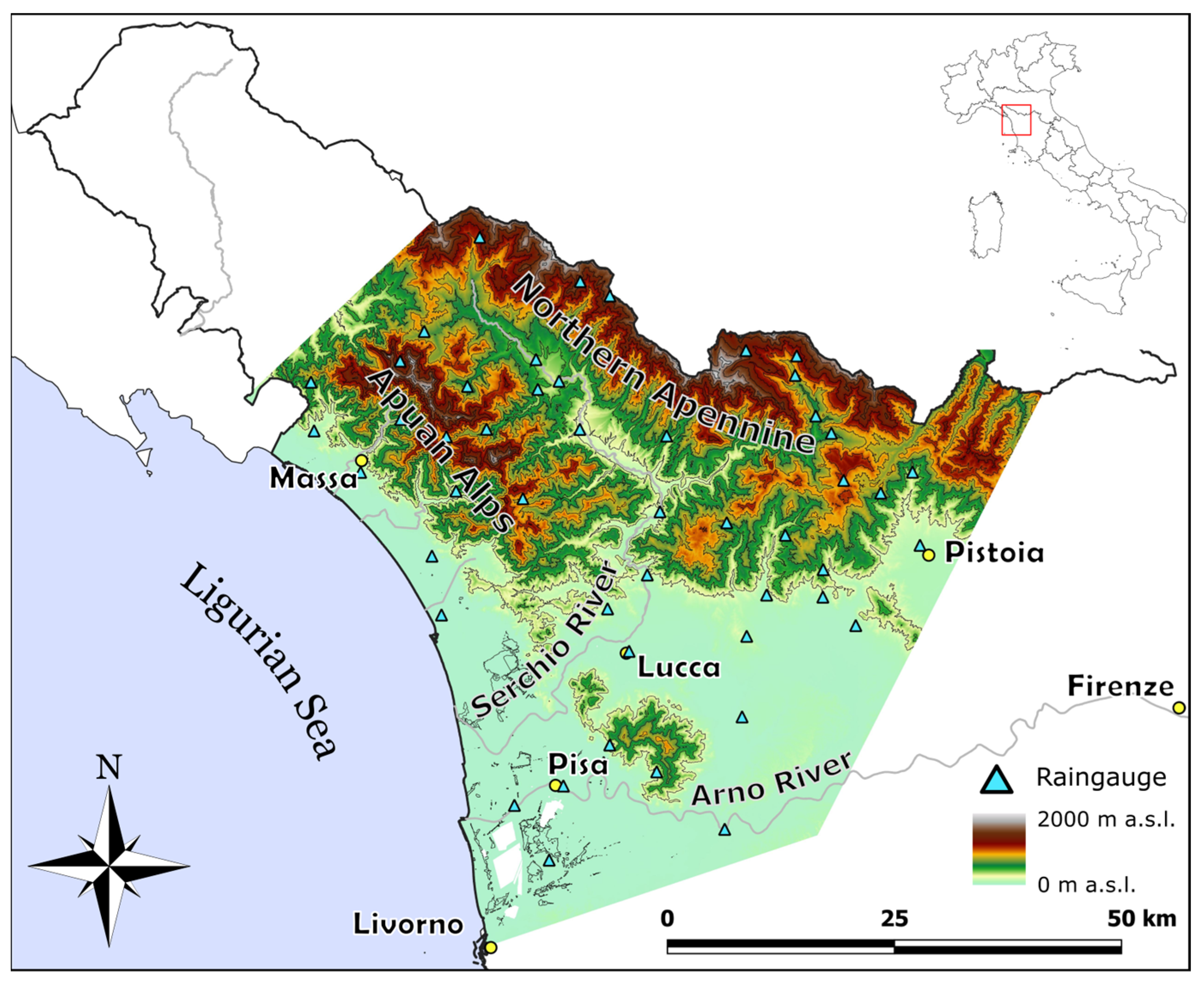
Figure 1. Topographic map of the study area. The selected rain gauges are indicated.
Water 16 02866 g001
Figure 2. Mean annual precipitation map for the study area related to the 1990–2019 period. The top-right graph shows the results of the cross-validation procedure of the interpolation (outlier rain gauges in orange squares in the interpolated observed plot). The dashed lines highlight the four sub-areas.
Water 16 02866 g002
Figure 3. The graph displays the average of the Mann–Kendall S statistic for all the rain gauges and the number of rain gauges with a p-value lower than 0.05 for each of the 30-year time windows. Also, the horizontal green–red bars in the background map display the Mann–Kendall S statistic for each rain gauge for each 30-year time window.
Water 16 02866 g003
Figure 4. Differences in MAP between the 1990–2019 and 1921–1970 periods for each considered rain gauge are reported along with the associated t-test p-value.
Water 16 02866 g004
Figure 5. Differences in MAP vs. elevation of all rain gauges divided into (a) Area 1, (b) Area 2, (c) Area 3, and (d) Area 4. Black lines correspond to the standard deviation in MAP differences. The blue lines correspond to the linear regression models.
Water 16 02866 g005
Figure 6. Differences between the MAP in the 1990–2019 and 1921–1970 periods. The legend of rain gauge symbols colors and shapes is the same of Figure 4.
Water 16 02866 g006
Table 1. Regression parameters and statistics for each MAP difference vs. elevation regression in the four areas. (‘*’: statistically significant values).
n. of Rain gaugesIntercept [mm]Intercept p-ValueCoeff. [mm/m]Coeff. p-ValueR2χ295% C.I. for χ2
Area 19−240.44−0.370.009 *0.656.0 *[2.2, 14.1]
Area 218−620.03−0.350.002 *0.4617.1 *[8, 26.3]
Area 316−1030.18−0.090.40.0634.9[6.6, 23.7]
Area 419−700.002−0.030.80.0023.4[8.7, 27.6]
Disclaimer/Publisher’s Note: The statements, opinions and data contained in all publications are solely those of the individual author(s) and contributor(s) and not of MDPI and/or the editor(s). MDPI and/or the editor(s) disclaim responsibility for any injury to people or property resulting from any ideas, methods, instructions or products referred to in the content.