Abstract
Climate change affects the water cycle, water resource management, and sustainable socio-economic development. In order to accurately predict climate change in Weifang City, China, this study utilizes multiple data-driven deep learning models. The climate data for 73 years include monthly average air temperature (MAAT), monthly average minimum air temperature (MAMINAT), monthly average maximum air temperature (MAMAXAT), and monthly total precipitation (MP). The different deep learning models include artificial neural network (ANN), recurrent NN (RNN), gate recurrent unit (GRU), long short-term memory neural network (LSTM), deep convolutional NN (CNN), hybrid CNN-GRU, hybrid CNN-LSTM, and hybrid CNN-LSTM-GRU. The CNN-LSTM-GRU for MAAT prediction is the best-performing model compared to other deep learning models with the highest correlation coefficient (R = 0.9879) and lowest root mean square error (RMSE = 1.5347) and mean absolute error (MAE = 1.1830). These results indicate that The hybrid CNN-LSTM-GRU method is a suitable climate prediction model. This deep learning method can also be used for surface water modeling. Climate prediction will help with flood control and water resource management.
1. Introduction
Climate change affects water cycle, surface water, groundwater, hydrological changes, land water storage capacity, runoff, hydrological drought, global water scarcity, landslides, mudslides, soil erosion, air quality, agriculture, industry, ecosystems, socio-economic development, and human health [1,2,3,4,5,6,7,8]. Over the past century, global land precipitation variability has significantly increased and can be attributed to the role of anthropogenic greenhouse gas emissions [9,10]. The increasing extreme weather and climate events have resulted in a sharp increase in the global cost of natural disaster risks [11]. Rising rainfall intensity results in severe drying upstream with decreases in water yield versus increases therein downstream in the West River Basin [12]. Realizing carbon neutrality will help prevent climate disasters. Developing accurate tools for predicting climate change is crucial for building a more sustainable future world. Hydrological and hydraulic phenomena are strongly affected by the temporal distribution of precipitations, i.e., the same monthly rainfall amount leads to very different effects evenly spread or piled in a short lapse [13,14]. Accurate climate prediction contributes to disaster prevention and mitigation, climate change adaptation, and effective water resources management [15,16]. Our simulation results provide a new perspective and method for risk management under climate change and a useful reference for policymaking.
Climate prediction is a great and urgent need for mankind to prevent natural disasters [17]. However, climate change is characterized by the coexistence of multiple time scales, the high complexity of multiple climate modes, and the disturbance of nonlinear chaotic variability, which makes it face huge difficulties. However, the traditional climate prediction method (Earth System Model) can not overcome this problem, so it is difficult to improve the uncertainty and accuracy of climate prediction. The physical climate model is limited to known and fully understood physical processes. It encounters difficulties when dealing with ambiguous or insufficiently understood processes. In addition, the Process-based model requires a large amount of input data, has high computational costs, and may exhibit lower performance due to incomplete inputs [18].
Data-driven artificial intelligence (AI) and ANNs are widely applied in COVID-19, air pollution index, PM2.5, and PM10 [19,20,21,22,23,24,25,26]. Emerging deep learning (DL) methods better utilize the spatial and temporal structures in data, addressing the limitations of traditional machine learning analysis methods in multiple scientific tasks, particularly when dealing with complex, dynamic, and spatially correlated data [27]. AI achieves reliability in predicting global extreme floods in ungauged watersheds [28]. ANNs perform the best in predicting rainfall occurrence and intensity among machine learning models [29]. The BPANN, LSTM, and Bidirectional LSTM (BiLSTM-attention) models have achieved higher accuracy in predicting changes in regional land water storage [30]. ANN and wavelet ANN (WANN) are used for groundwater forecasting [31]. WT (wavelet)-M5-ANN method is used to predict the rainfall-runoff phenomenon [32]. RNN is developed to predicate nonlinear daily runoff in the Muskegon River and the Pearl River [33]. GRU for short-term runoff prediction performs equally well as LSTM [34]. CNNs are developed for daily runoff forecasting [35]. The CNN, LSTM, and convolutional LSTM (ConvLSTM) are used to design HydroDL for runoff prediction in the Yalong River [36]. LSTM excels at capturing long-term dependencies in hydrological time series, making it suitable for analyzing complex hydrological time series. LSTM-grid is a grid-based hydrological prediction model that can predict hydrological runoff in seven major river basins of the Third Pole [37]. SWAT-LSTM improves streamflow simulations [38]. CNN-LSTM and GRU are combined to predict long and short-term runoff [39].
Data-driven AI and deep learning (DL) have improved the level of weather and climate prediction [40,41,42,43,44,45]. AI and deep learning (DL) also can improve Earth system models (numerical learning models) by learning from observed and simulated data [46,47]. Machine learning methods provide new approaches for modeling the Earth system [18]. It is possible to predict the trends of climate development in the coming months by utilizing the climate change patterns (temperature and precipitation) of the past few months. NeuralGCM combines machine learning and atmospheric dynamics numerical models. This hybrid model can accurately predict weather and climate, and the predictions provided by Neural GCM are clearer than those of GraphCast, and its accuracy is comparable to ECMWF-HRES, but the required computing power is much lower than ECMWF-HRES [48]. ANNs are used to predict the Indian Ocean Dipole (IOD). The ANN models perform far better than the models of the North American Multi-Model Ensemble (NMME) [49]. ANNs are developed to forecast solar radiation (SR). Bayesian Regularization (BR) algorithm-trained ANN models outperform other algorithm-trained models [50]. Convolutional neural networks (CNN) are used to create dynamically consistent counterfactual versions of historical extreme events [51]. CNN is also used to predict extreme floods and droughts in East Africa [52]. The deep learning (DL) method is used to investigate the predictability of the MJO-related western Pacific precipitation. The DL model consists of two max-pooling and three convolutional layers [53]. Convolutional LSTM is used for tropical cyclone precipitation nowcasting [54]. The performance improvement of FuXi-S2S is mainly attributed to its superior ability to capture forecast uncertainty and accurate prediction [55]. Therefore, using deep learning (DL) methods may be a solution for accurately predicting climate change in Weifang, and this study investigates the efficiency and accuracy of the deep learning (DL) models. The research objectives are (1) to evaluate the simulation and prediction performance of different deep learning (DL) models and (2) to study the ability of deep learning (DL) to capture climate change without prior knowledge.
In summary, a hybrid prediction model for climate change based on a multi-model stacking ensemble, CNN, LSTM, and GRU, named CNN-LSTM-GRU, is proposed. The primary contributions of this paper lie in:
- (1)
- Wavelet transform is introduced to determine the input variables of the deep learning models.
- (2)
- By analyzing the performance of different deep learning models, CNN, LSTM, and GRU are used to form a hybrid model.
- (3)
- CNN-LSTM-GRU can simultaneously focus on both local and global information of the climate change time series, improving its ability to recognize complex patterns in the climate change time series.
- (4)
- The proposed hybrid CNN-LSTM-GRU model has higher prediction accuracy than a single method.
The rest of this study is organized as follows: Section 2 outlines the data sources and provides a description of deep learning models. In Section 3, we analyze the experimental results, comparing the performance of our model against other models. Section 4 discusses the study’s limitations. Finally, in Section 5, we draw conclusions and present future research.
2. Materials and Methods
2.1. Study Area and Data
Weifang is located in the central part of Shandong Province (Figure 1), with continental climate. In 2023, the population of Weifang City is 9.37 million, with a regional GDP of 760.6 billion yuan.
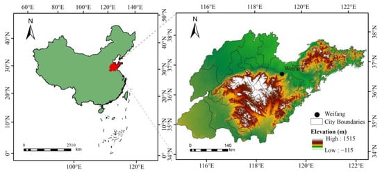
Figure 1.
Location Map of Weifang city.
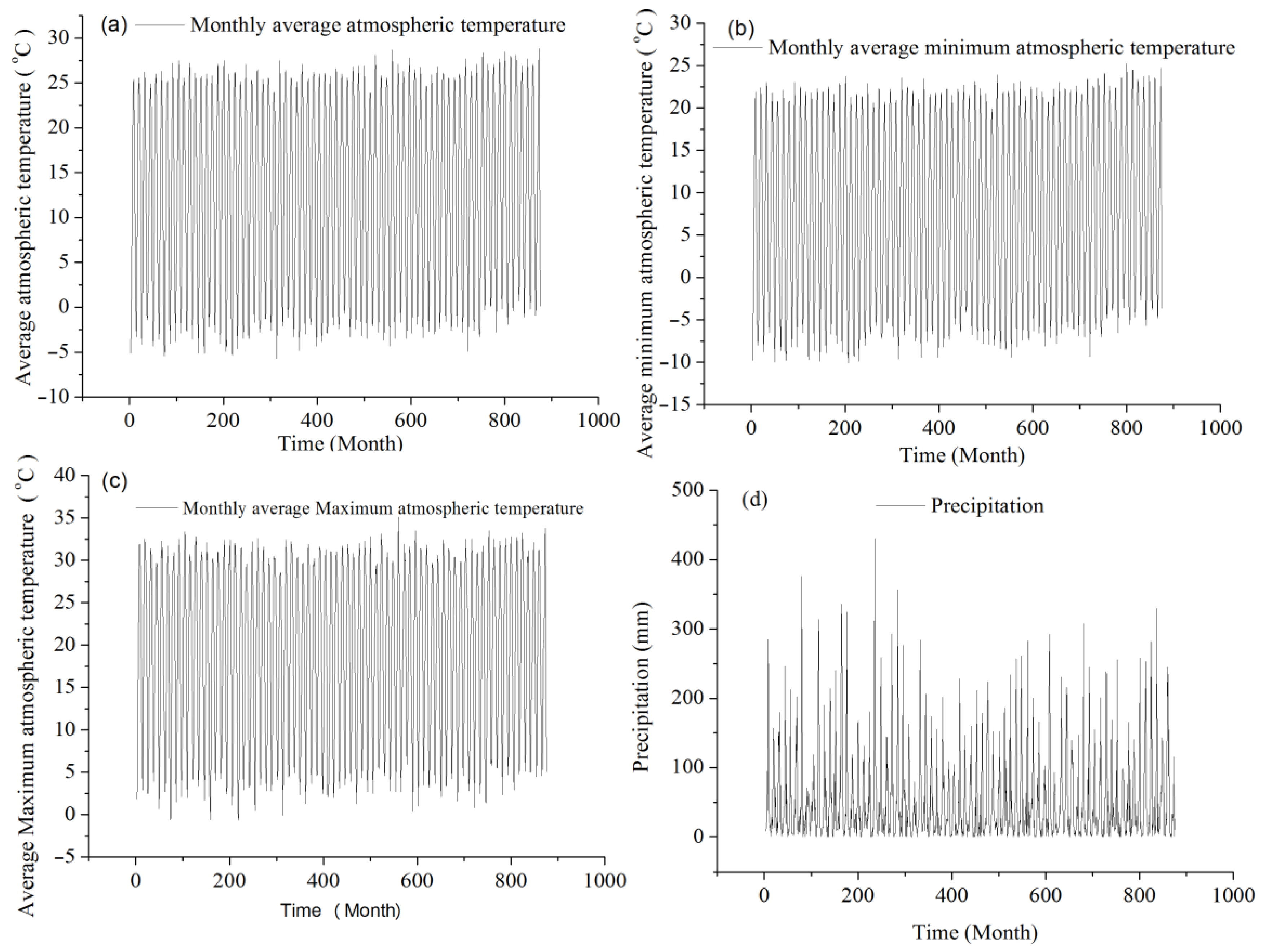
The monthly climatological data (1 January 1951–31 December 2023) in Weifang City were obtained from the China Meteorological Administration. The data include monthly average air temperature (MAAT), monthly average minimum air temperature (MAMINAT), monthly average maximum air temperature (MAMAXAT), and monthly precipitation (MP) (Figure 2). The datasets are divided into three parts: training (from January 1951 to May 2009), verification (from June 2009 to August 2016), and predicting (from September 2016 to December 2023).
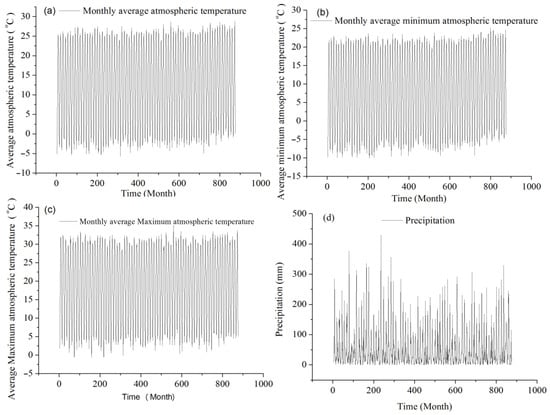
Figure 2.
Original data on monthly climate change in Weifang city from 1951 to 2023. (a) change of monthly average minimum atmospheric temperature, (b) change of monthly average minimum atmospheric temperature, (c) change of monthly average maximum atmospheric temperature, (d) change of monthly precipitation.
2.2. Data Standardization
Standardization can improve the training speed of deep learning (DL) models. The definitions of qm are as follows:
where Qm means the climate series at the time m; Qmin, and Qmax mean the minimum and maximum values of the climate sequence, respectively; and qm is the normalized climate results.
2.3. Artificial Neural Network (ANN)
ANN is structurally inspired by the human brain, where multiple layers of neurons are connected together through a network from one layer to another based on the received information and expected results. Similarly, the ANN architecture consists of 11 neural nodes called “channels” that transform climate indicators. ANN has multiple layers linked by channels containing different weights. ANN is suitable for various tasks, including classification and regression. ANN has a strong representation ability and can capture complex nonlinear relationships between the dependent and explanatory variables [56]. Data-driven AI is a broad concept that encompasses all technologies and methods aimed at simulating human intelligence. ANN is a specific technical means of implementing AI, particularly performing well in pattern recognition and prediction tasks.
2.4. Recurrent Neural Network (RNN)
RNN is a type of recursive NN used for processing sequential data. In RNN, information circulates in a sequential manner throughout the network, with each node (recurrent unit) connected into a chain. RNN can effectively model sequential data and generate outputs. Two RNN variants (LSTM and GRU) maintain excessively prolonged dependencies in the hidden state [57].
2.5. Long Short-Term Memory (LSTM)
LSTM is a specialized architecture for representing time series using RNNs. LSTM has a wide range of interdependencies, making it more accurate than traditional RNNs. The backpropagation algorithm in RNN design has led to the problem of error backflow. Unlike RNN, LSTM includes memory blocks as different units in the cyclic hidden layer. A storage block is composed of self-connected storage units that enable it to store the network state. In LSTM, three gate functions, namely input, forget, and output gates, are used to control the input, stored, and output values. LSTM controls the flow of information through gate mechanisms, making it suitable for processing and modeling time series data. LSTMs can not only consider the time lag and memory effects of climate data but also capture long-distance spatial context, thereby improving the predictive ability and accuracy of the models. LSTMs demonstrate their advantages in processing time series data, particularly in predicting complex dynamic processes related to environmental and climatic conditions [58].
2.6. Gate Recurrent Unit (GRU)
GRU is a LSTM variant. Both models belong to RNNs, and they are specialized in processing nonlinear sequence data. GRU is a more efficient variant, with a simpler structure and better performance. GRU only has two gates (update and reset gates). GRU is similar to LSTM, but with a simpler structure. It is also suitable for processing sequential data, with update gates and reset gates to regulate the flow of information. GRU has higher computational efficiency compared to LSTM and may perform better on medium-sized datasets [59].
2.7. Convolutional Neural Network (CNN)
CNN has become a prominent time series prediction technique. Firstly, one-dimensional climate data are input, and after convolution and pooling operations, the extracted high-dimensional climate data are mapped to a low-dimensional feature through a fully connected layer. Finally, by applying a nonlinear function, the predicted value is output. It can capture local data features and exhibit strong robustness and generalization ability. In addition, CNN is particularly effective in processing process data constructed with a class array topology. CNN can extract features from time series within different time windows [60].
2.8. Hybrid Model
CNN-GRU combines the advantages of CNN and GRU. CNN is used to process multi-channel inputs of multivariate time series and can effectively capture spatial relationships between input features. GRU can capture long-range dependencies in sequences.
CNN-LSTM takes the feature sequence extracted by CNN as input and models the sequence through the LSTM model. CNN-LSTM combines the advantages of CNN in extracting spatial features and LSTM in handling temporal dependencies. This model can effectively handle complex time-series data and provide accurate regression prediction results, demonstrating good performance and generalization ability in climate prediction.
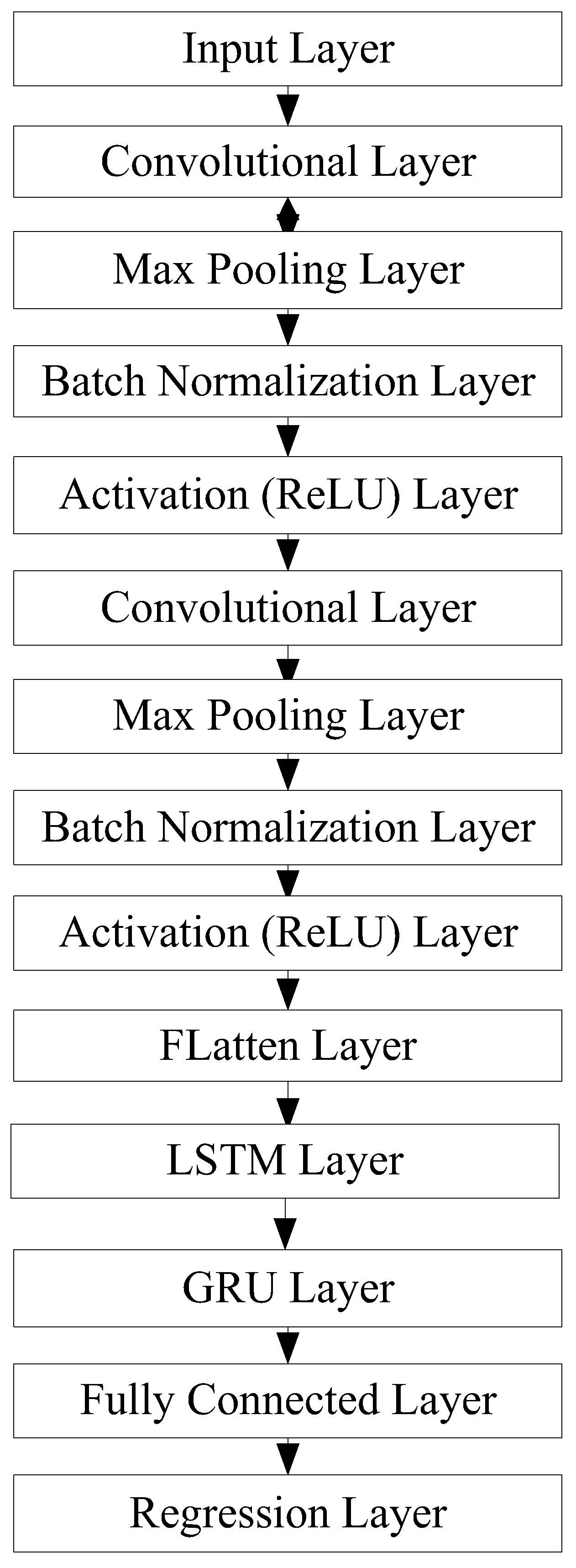
CNN-LSTM-GRU combines the advantages of CNN, LSTM, and GRU (Figure 3). It extracts implicit features by sequentially inputting time-series data sequences into the CNN network and then inputting the data into the LSTM and GRU networks for temporal dependency and pattern feature extraction. Finally, it outputs the prediction results.
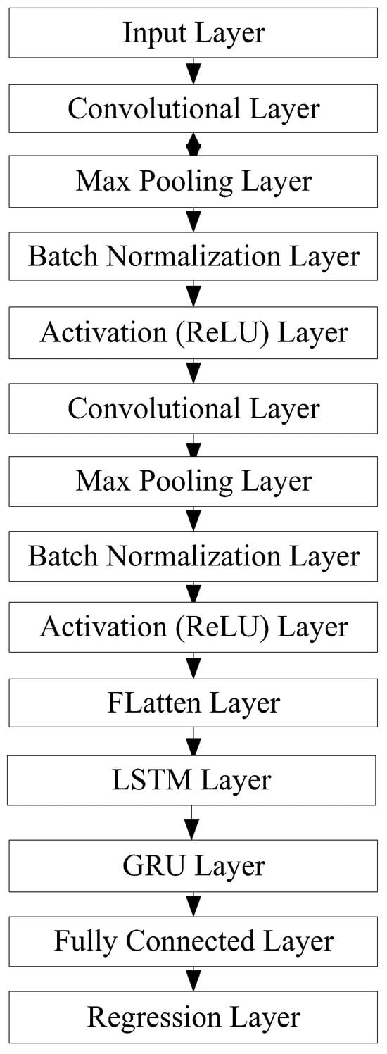
Figure 3.
CNN-LSTM-GRU model.
2.9. Model Evaluation Indicators
Three evaluating indicators (metrics) are applied to validate the deep learning model’s performance: R (correlation coefficient), RMSE (lowest root mean square error), MAE (mean absolute error), and MAPE (mean absolute percentage error). RMSE measures the average difference between the monthly climate values predicted by a deep learning method and the actual monthly climate values, MAE measures the average absolute differences between the forecasted monthly climate values and the actual monthly climate target values, and R measures the linear correlation between two variables [61].
The equations are shown in the following:
where I denotes the number of climate data series. Om and are the prediction value and the average of predicted values, respectively.
2.10. Cross-Validation
The results of the deep learning models based on the 10-fold-cross-validation technique are tested in this study. We randomly divide the climate dataset into ten equal climate time subsets. In each run, nine climate time subsets are utilized to build the deep learning model, while the remaining climate time subsets are utilized for prediction. The average accuracy of ten iterations is treated as the deep learning model precision value.
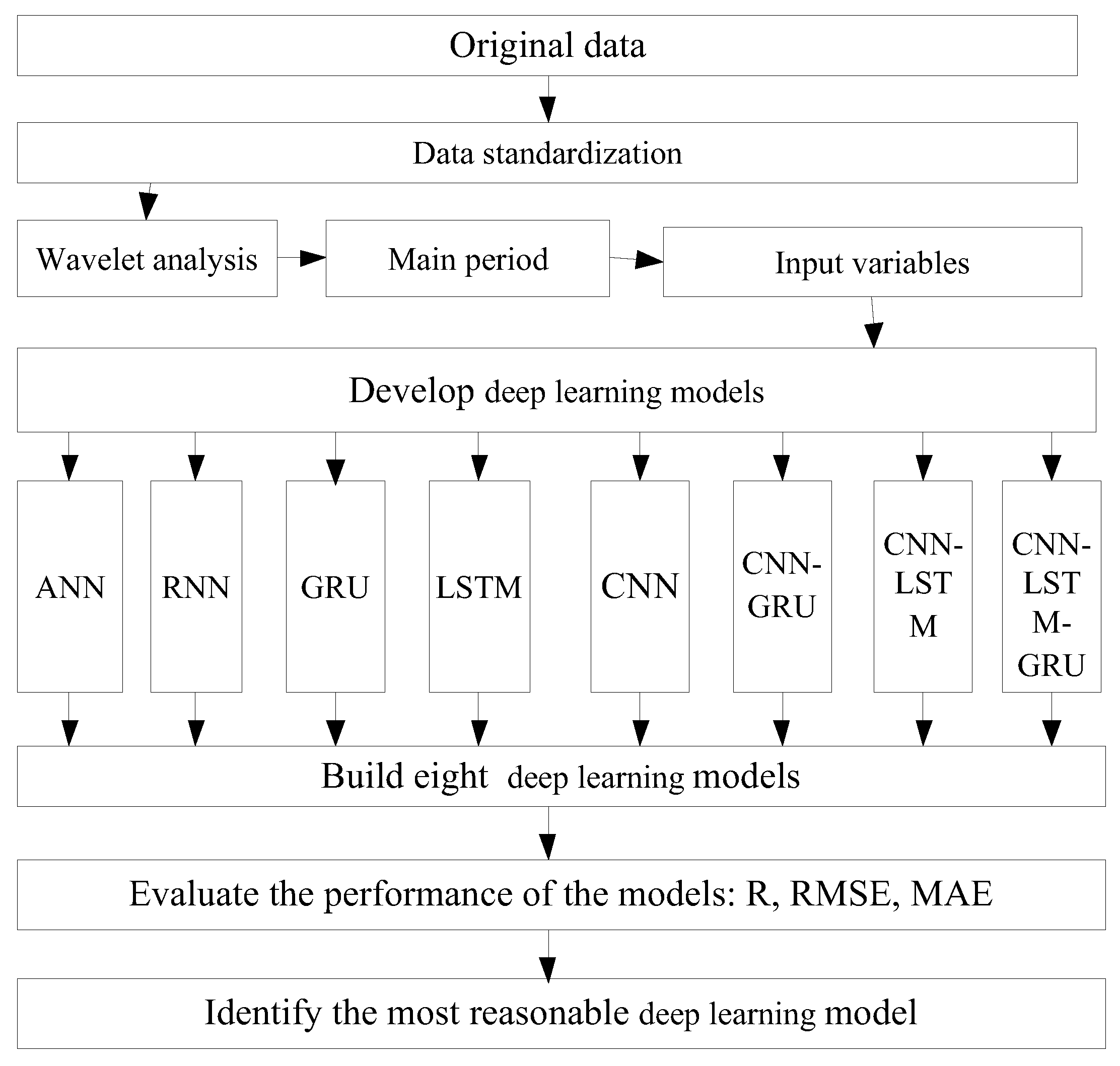
The process of this study is shown in Figure 4. We trained the model using 690 sets of data, then tested it using 87 sets of data, and finally made predictions using 87 sets of data. We evaluated all deep learning models using evaluation metrics and identified the best predictive model. By using a backpropagation algorithm to calculate gradients and update model parameters, the performance of the model is iteratively optimized. Mini-batch training can be used during the training process. The loss function is used to measure the difference between the predicted results of the model and the true values, and the appropriate optimization algorithm, Adam, is selected to minimize the loss function. The Adam optimizer is a variant of the gradient descent algorithm. It is used to update the weights of deep neural networks. It combines a stochastic gradient descent (SGD) algorithm and an adaptive learning rate algorithm, which can converge quickly and reduce training time. It calculates the independent adaptive learning rate for each parameter without the need to adjust the size of the learning rate. It can adaptively adjust the learning rate based on historical gradient information so that using a larger learning rate in the early stages of training can quickly converge, and using a smaller learning rate in the later stages of training can more accurately find the minimum value of the loss function. It can adjust momentum parameters to balance the impact of the previous gradient and the current gradient on parameter updates, thereby avoiding premature entry into local minima. It normalizes parameter updates to ensure that each parameter update has a similar magnitude, thereby improving training performance. It combines the idea of L2 regularization to regularize parameters during updates, thereby preventing neural networks from overfitting training data. Overall, It can quickly and accurately minimize the loss function, improving the training performance of deep neural networks.
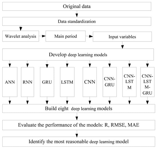
Figure 4.
The flowchart of this study.
3. Results
3.1. Annual Climate Change in Weifang City
The annual average atmospheric temperature (AAAT) and annual average minimum temperature (AAMINT) in Weifang City in 2023 are 1.9 °C and 2.3 °C higher than those in 1951, respectively (Figure 5). The warming rates of annual average air temperature, average air temperature, average minimum air temperature, and average maximum air temperature are respectively 0.293 °C/10 years, 0.344 °C/10 years, and 0.147 °C/10 years from 1951 to 2023. The growth rate of annual precipitation was 6.39 mm/10 years. The results indicate that both air temperature and precipitation show an increasing trend in Weifang City. 2023 is the hottest year on record worldwide. The global average near-surface temperature is 1.45 °C higher than the pre-industrial baseline (1850 to 1900) (WMO). The recent rate of global surface warming during 50 (1974–2023) years is 0.19 °C/decade [62]. The national average temperature in 2023 is 10.71 °C, which is the highest since 1951 in China. The national average precipitation in 2023 is 615 mm, which is 3.9% less than usual and the second lowest since 2012. From 1951 to 2021, the annual average surface temperature in China showed a significant upward trend, with a warming rate of 0.26 °C/decade. The warming rate in Weifang City is higher than that of the world and China. Local factors such as urbanization and land use change have led to climate change in Weifang City.
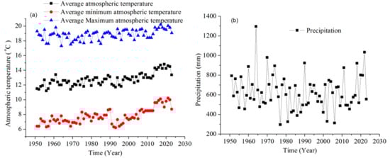
Figure 5.
Annual climate change in Weifang from 1951 to 2023. (a) annual change of average minimum air temperature, average minimum air temperature, and average maximum atmospheric temperature; (b) annual change of precipitation.
3.2. The Cyclicality of Climate Change
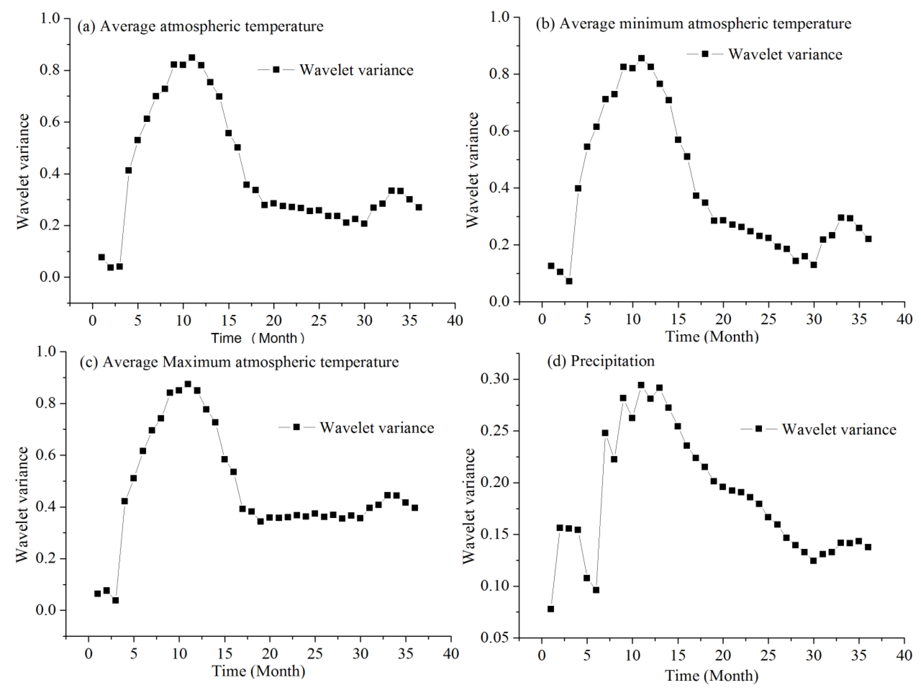
The periods of monthly climate change in Weifang city are calculated using wavelet analysis (Figure 6). The wavelet variance determines the main periods of monthly climate change. There is a maximum peak of 11. These are the periods of monthly average air temperature, monthly average minimum air temperature, monthly average maximum air temperature, and monthly precipitation. The monthly variation of temperature is mainly influenced by solar radiation, especially the seasonal variation of solar radiation. The solar activity cycle is approximately 11 years. Therefore, the input variables of the deep learning models are 11.
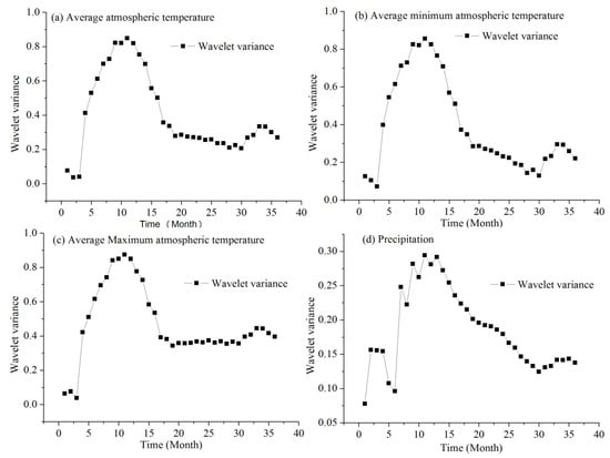
Figure 6.
Periodic change of monthly climate in Weifang city. (a) periodic change of monthly average minimum atmospheric temperature (MAAT), (b) periodic change of monthly average minimum atmospheric temperature (MAMINAT), (c) periodic change of monthly average maximum atmospheric temperature (MAMAXAT), (d) periodic change of monthly precipitation.
3.3. Hyperparameter Information of the Deep Learning Models
The selection of features is critical for model training and reproducibility. We calculate the correlation coefficients (R) between the 11 input variables and the output variable. The ranges of correlation coefficients for precipitation, MAAT, MAMINAT, and MAMAXAT are 0.40511–0.4299, 0.85371–0.8540, 0.8539–0.8548, 0.84242–0.8440, respectively. Therefore, 11 variables are used as inputs for the model. The hyperparameters in the deep learning models are selected in Table 1. We use the grid search to optimize parameters and achieve prediction accuracy. An ANN has two hidden layers (HL). CNN contains nine HLs with 50 neurons. The activation functions (AFs) of RNN are tansig and purelin, the learning rate (LR) is 0.005, the number of epochs is 200, the batch size (BS) is 12, the kernel size (KS) is 3, the max-pooling (MP) is 2, the convolution filters (CFs) are 12 and 12, and the Optimizer is Adam.

Table 1.
Hyperparameters information of the deep learning models.
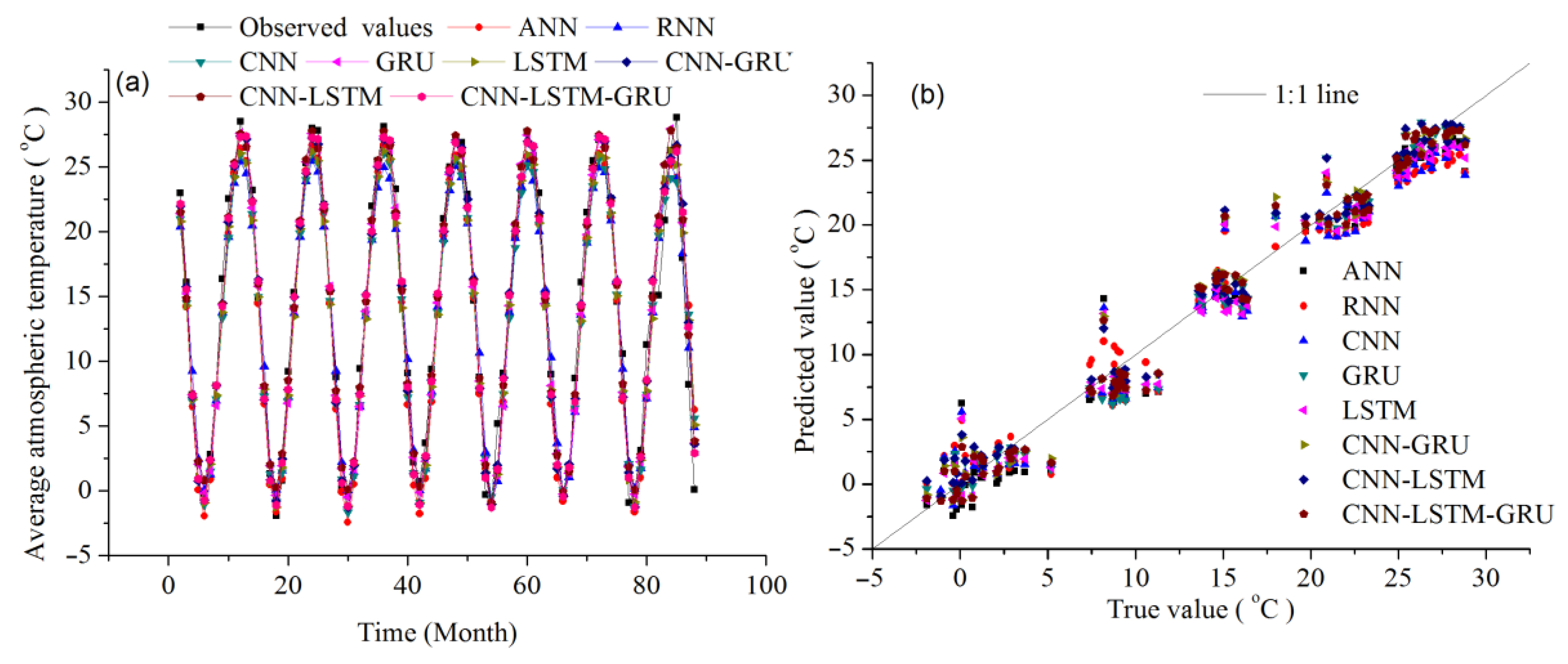
3.4. Prediction of MAAT in Weifang City
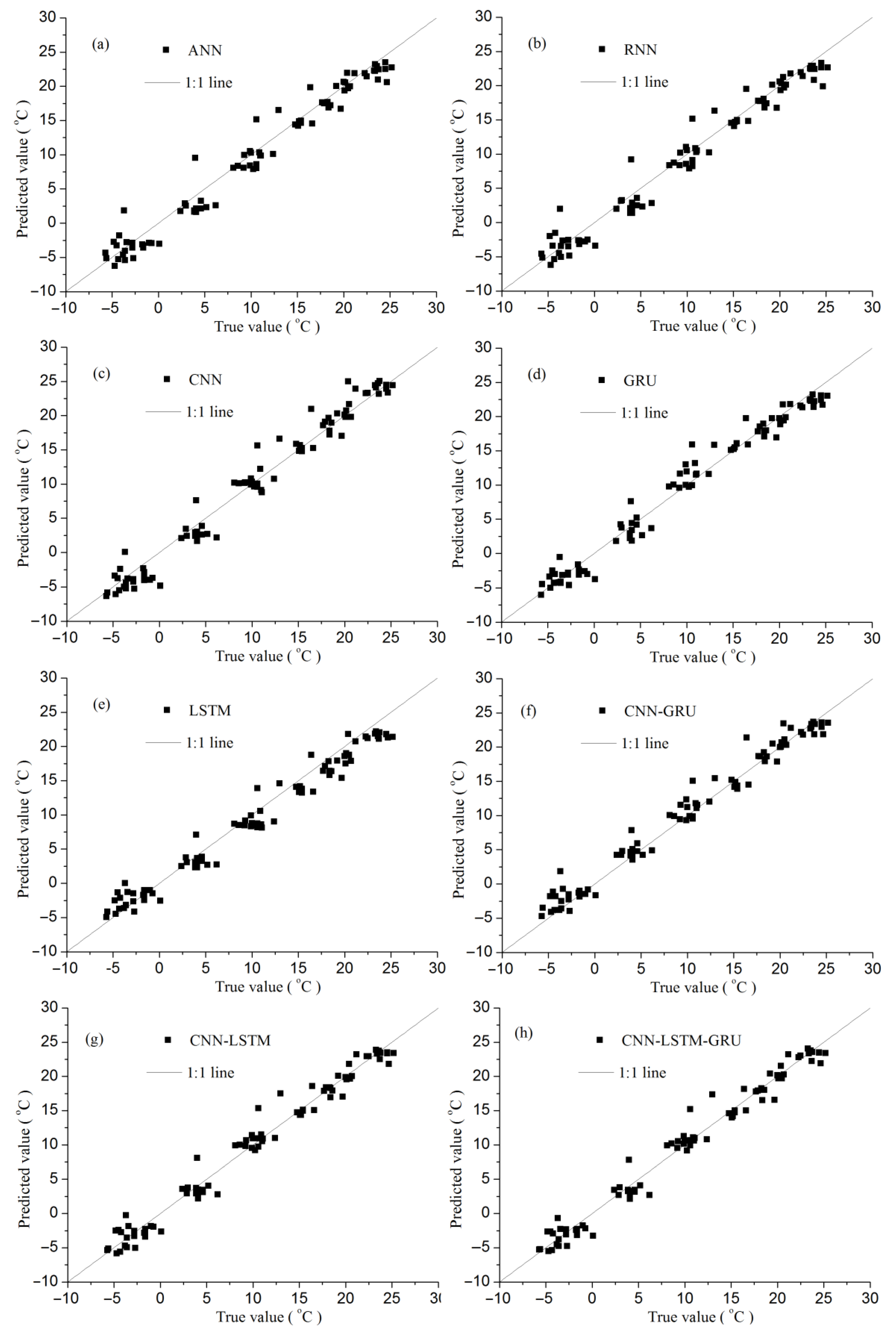
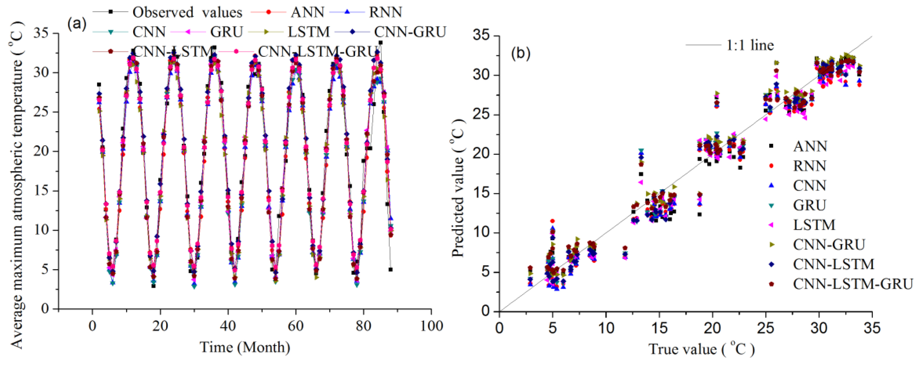
The deep learning (DL) models are developed and compared to predict monthly average atmospheric temperature (MAAT). Although all models meet reasonable prediction requirements, the performance of the CNN-LSTM-GRU is superior to other models, with R (0.9879), RMSE (1.3277), and MAE (1.1830), respectively (Table 2). Figure 7 compares the observed and predicted values for the different deep learning models in Weifang during the prediction period. The CNN-LSTM-GRU can efficiently capture the monthly average air temperature (MAAT) trend. Figure 8 utilizes an aspect scheme to plot each model on its own plane for easier performance comparison.
Table 2.
Performance statistics of different deep learning models for simulated MAAT.
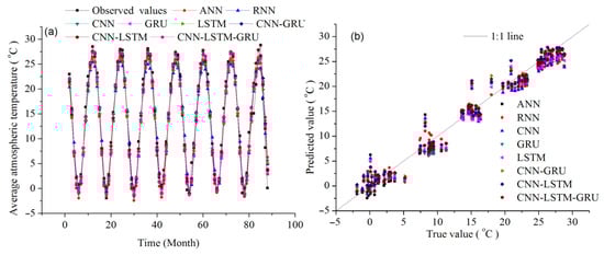
Figure 7.
The prediction results of monthly average air temperature (MAAT) in Weifang from September 2016 to December 2023. (a) Plot, (b) Scatterplot.
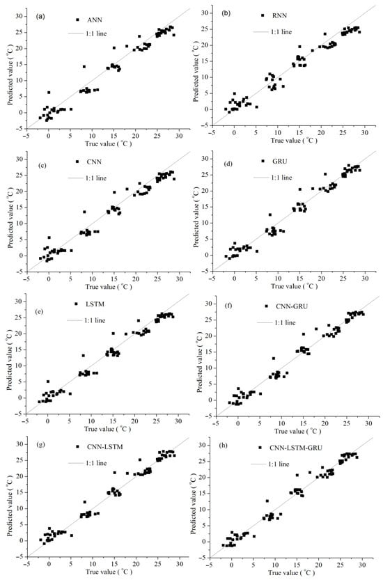
Figure 8.
Comparison of observed and predicted MAAT values for each model. (a) results of ANN, (b) results of RNN, (c) results of CNN, (d) results of GRU, (e) results of LSTM, (f) results of CNN-GRU, (g) results of CNN-LSTM, (h) results of CNN-LSTM-GRU.
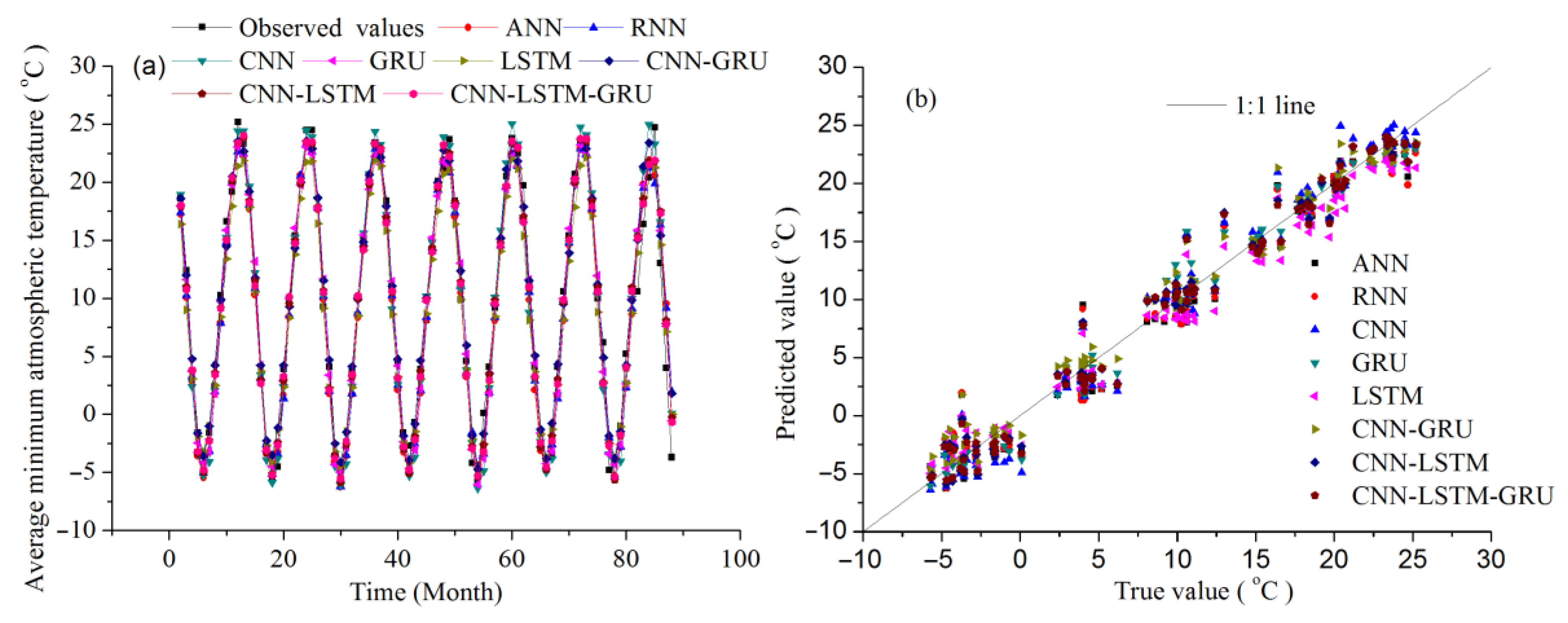
3.5. Prediction of MAMINAT in Weifang City
Table 3 shows the results of different deep learning (DL) models. The hybrid CNN-LSTM-GRU in the predicting phase has better assessment criteria, with R = 0.9886, RMSE = 1.4856 °C, and MAE = 1.1218 °C, respectively. Figure 9 and Figure 10 show results comparing the measured and predicted monthly average minimum air temperature (MAMINAT) using different DL models. Also, the forecasted values of CNN-LSTM-GRU are closer to the measured values compared to the ANN, RNN, CNN, GRU, LSTM, CNN-GRU, and CNN-LSTM models.
Table 3.
Performance statistics of different deep learning models for simulated monthly average minimum air temperature (MAMINAT).
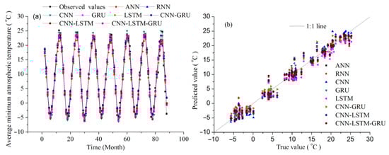
Figure 9.
The prediction results of monthly average minimum air temperature (MAMINAT) in Weifang from September 2016 to December 2023. (a) Plot, (b) Scatterplot.
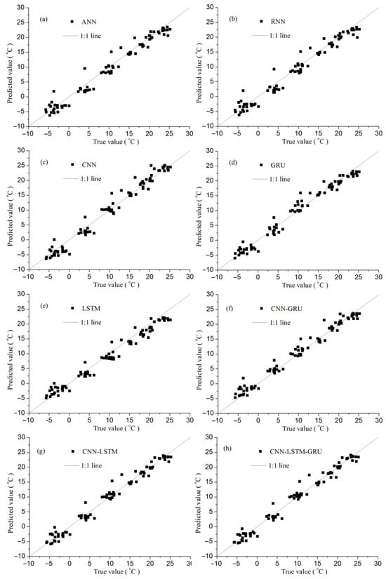
Figure 10.
Comparison of observed and predicted MAMINAT values for each model. (a) results of ANN, (b) results of RNN, (c) results of CNN, (d) results of GRU, (e) results of LSTM, (f) results of CNN-GRU, (g) results of CNN-LSTM, (h) results of CNN-LSTM-GRU.
3.6. Prediction of MAMAXAT in Weifang City
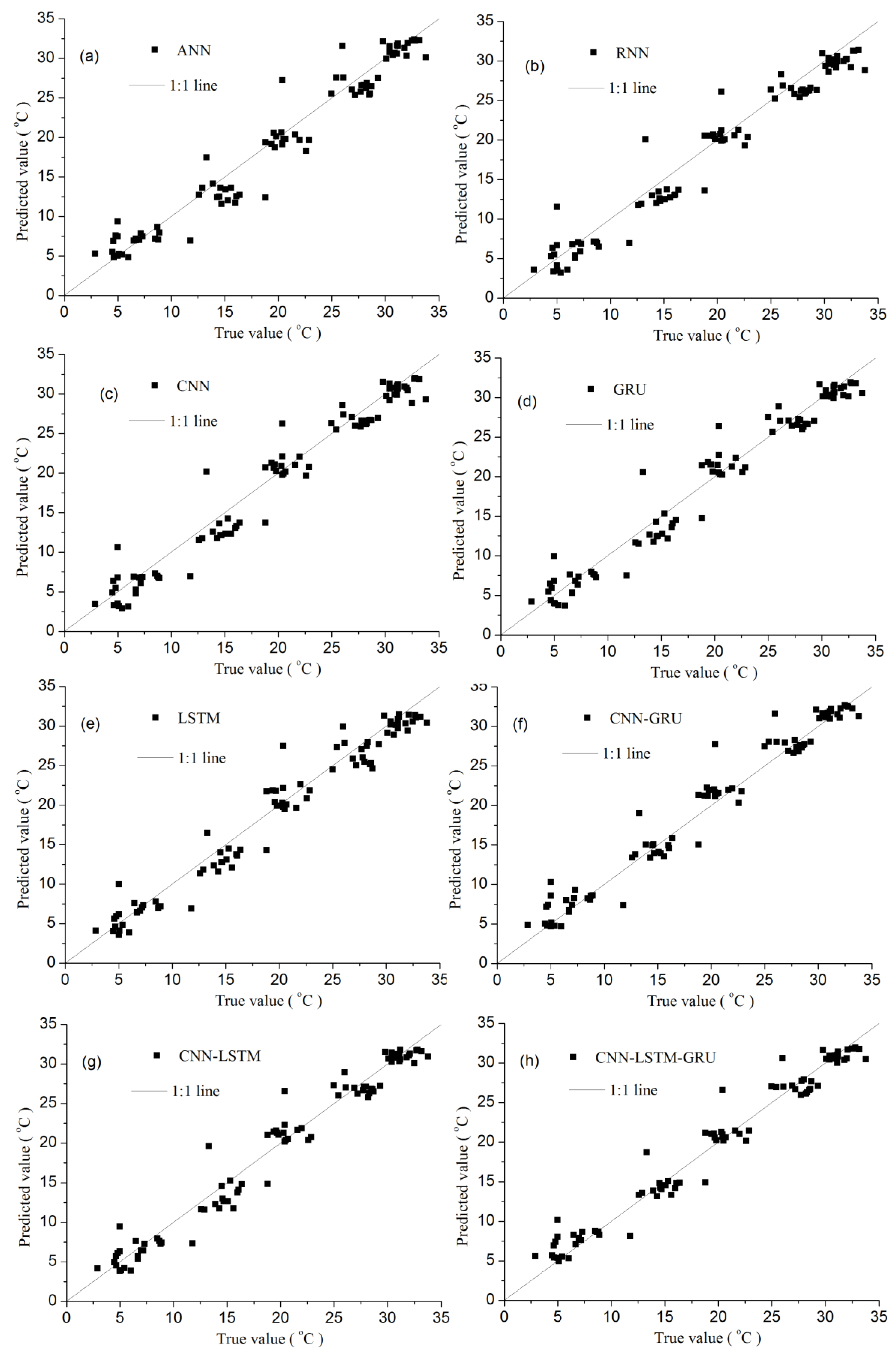
The CNN-LSTM-GRU model shows the best performance in predicting MAMAXAT with R (0.9832), RMSE (1.7843 °C) and MAE (1.2523 °C), while the CNN-LSTM model also showed the better performance in forecasting MAMAXAT than other deep learning models (Table 4). Figure 11 and Figure 12 show the measured and predicted monthly average maximum atmospheric temperature (MAMAXAT) using deep learning models in 2016–2023, demonstrating that the past 11 months’ data play a vital role in the MAMAXAT prediction.
Table 4.
Performance statistics of different deep learning models for simulated monthly average maximum atmospheric temperature (MAMAXAT).
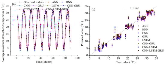
Figure 11.
The prediction results of monthly average maximum air temperature (MAMAXAT) in Weifang from September 2016 to December 2023. (a) Plot, (b) Scatterplot.
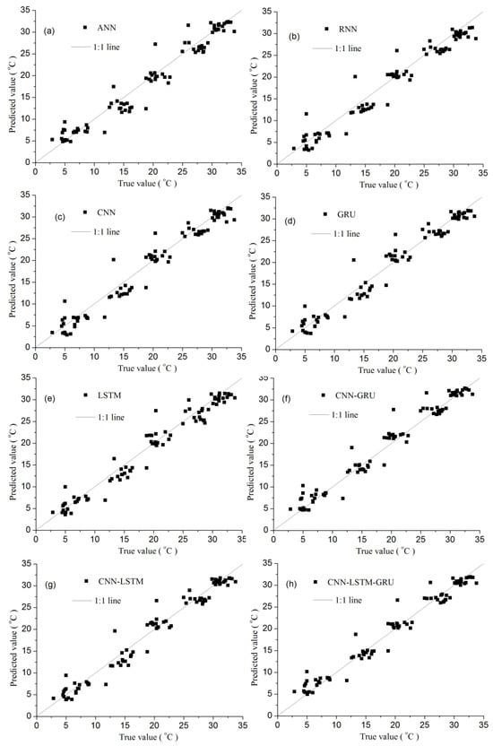
Figure 12.
Comparison of observed and predicted MAMAXAT values for each model. (a) results of ANN, (b) results of RNN, (c) results of CNN, (d) results of GRU, (e) results of LSTM, (f) results of CNN-GRU, (g) results of CNN-LSTM, (h) results of CNN-LSTM-GRU.
3.7. Prediction of Monthly Precipitation (MP) in Weifang City
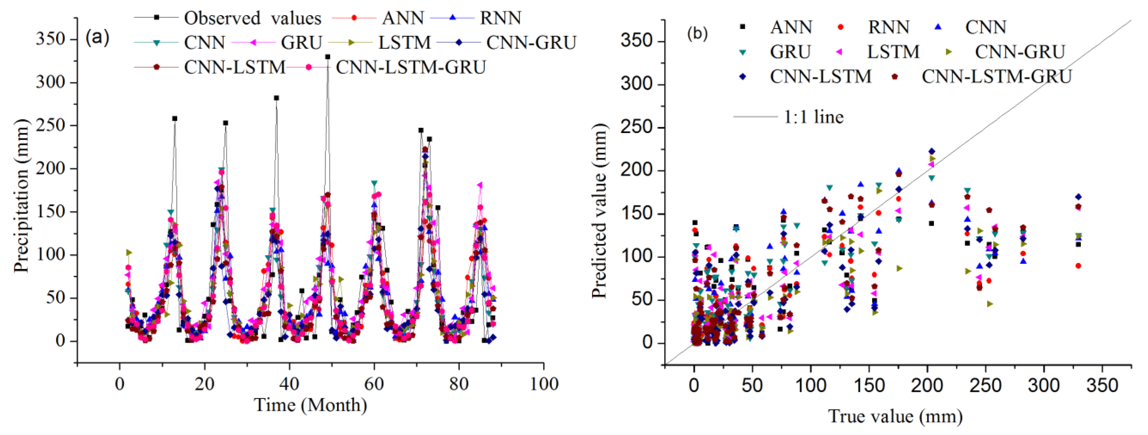
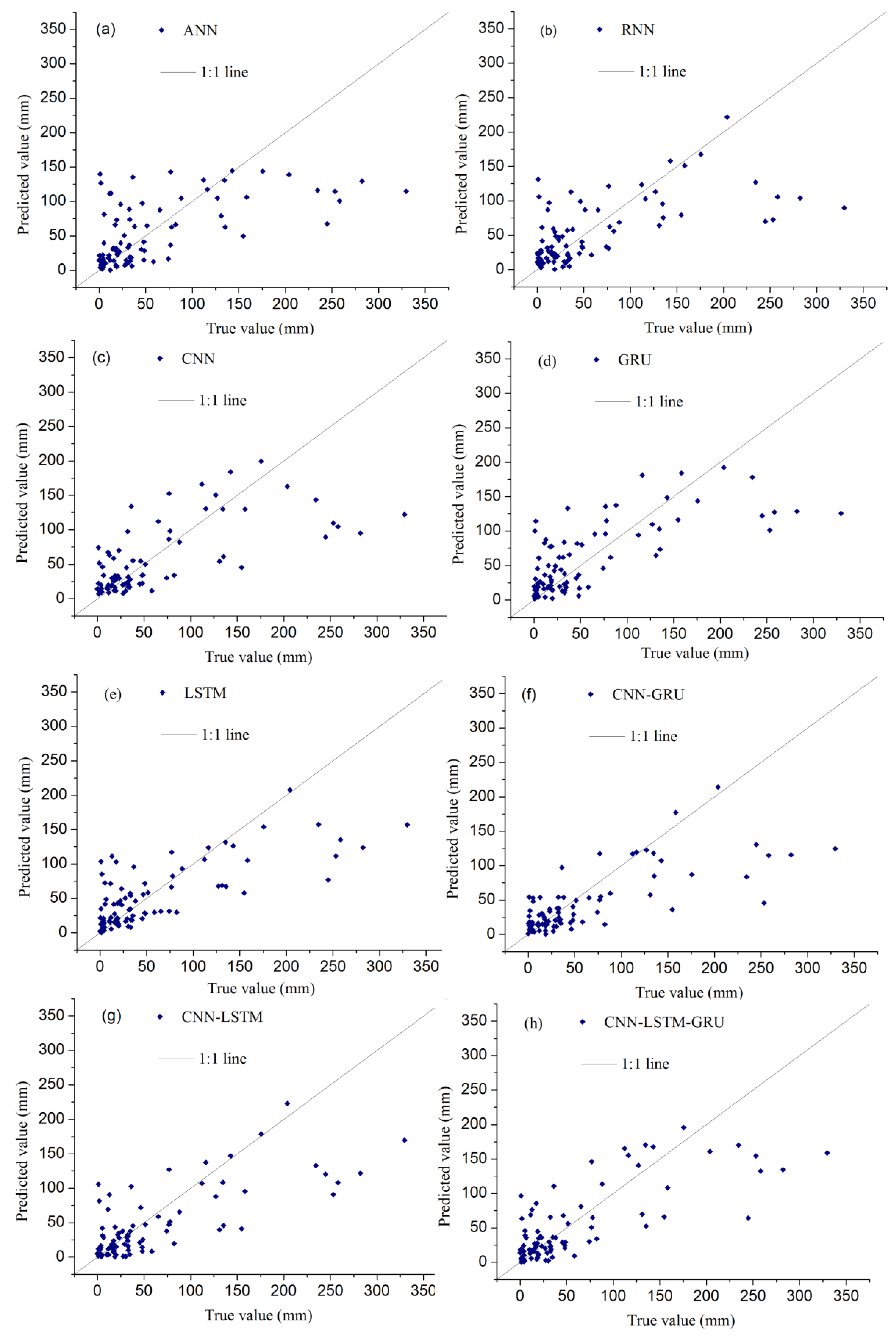
CNN-LSTM-GRU shows the best performance in predicting monthly precipitation (MP) with R (0.7629), RMSE (48.0323 mm), and MAE (31.1680 mm) (Table 5). Also, the CNN-LSTM model shows better performance in forecasting monthly precipitation (MP) than other deep learning models, which offer a high R of 0.7617, a low RMSE of 50.1189 mm, and a low MAE of 31.1853 mm. Figure 13 and Figure 14 show the measured and predicted monthly precipitation (MP) using different deep-learning models in 2016–2023. Comparing the predicted error to the one derived by month-specific averages, the relative error of CNN-LSTM-GRU is 44.722%. The result shows the potential enhancement from the proposed approach when compared to simple monthly averages from the dataset.
Table 5.
Performance statistics of different deep learning models for simulated monthly precipitation (MP).
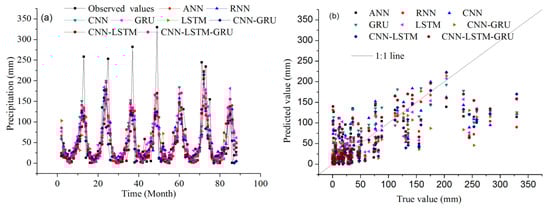
Figure 13.
The prediction results of monthly precipitation in Weifang City from September 2016 to December 2023. (a) Predicted results, (b) Scatter plots.
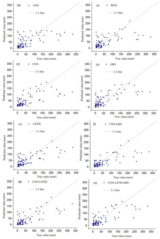
Figure 14.
Comparison of observed and predicted precipitation values for each model. (a) results of ANN, (b) results of RNN, (c) results of CNN, (d) results of GRU, (e) results of LSTM, (f) results of CNN-GRU, (g) results of CNN-LSTM, (h) results of CNN-LSTM-GRU.
4. Discussions
The obtained results of this study show that CNN-LSTM-GRU has the highest R values and the lowest RMSE and MAE values for the monthly climate prediction for all elements, including monthly average air temperature (MAAT), monthly average minimum air temperature (MAMINAT), monthly average maximum air temperature (MAMAXAT), and monthly precipitation (MP), while CNN-LSTM closely follows CNN-LSTM-GRU. From CNN-LSTM-GRU to ANN, the RMSE and MAE increase, and R decreases (Table 2, Table 3, Table 4 and Table 5). Therefore, deep learning model performance can be ranked as CNN-LSTM-GRU > CNN-LSTM > CNN-GRU > LSTM > GRU > CNN > RNN > ANN. The eight deep learning models have good generalization ability. CNN extracts multidimensional data features, GRU and LSTM, and has modeling capabilities for long-term dependencies in sequence data processing, and the CNN-LSTM-GRU hybrid model can further improve model prediction accuracy. The CNN-LSTM-GRU model provides a new predictable model for climate change. The hybrid model’s ability to predict air temperature and precipitation is crucial for water resource management and early-warning systems in flood risk management.
Many scholars have conducted extensive climate prediction work using AI and deep learning models [63,64,65]. ANN is used to forecast Air temperature in Ararat Valley (Armenia). The ANN has 87.31% accuracy in predicting the temperature [66]. Machine learning (ML) is proposed as a precise rainfall forecast model. LSTM outperforms CNN and GRU. The research demonstrates the superiority of LSTM in predicting rainfall [67]. LSTM is used to forecast urban air temperature in Hong Kong. Increasing the complexity of LSTM cannot further improve urban air temperature forecasting [68]. Three learning models are proposed to predict monthly precipitation in the Boyacá Department. The LSTM model outperformed others (ARIMA and RF-R), precisely replicating observed precipitation datasets, significantly reducing RMSE [69]. LSTM can preserve and learn sequential dependencies in precipitation time series datasets, so it simulates the inherently complex and nonlinear patterns. TISE-LSTM can predict precipitation and enhance performance in precipitation nowcasting [70]. ANN model performs average atmospheric temperature prediction and shows the lowest error [71]. LSTM performs significantly better than models in precipitation prediction with a coefficient of determination (R2) value of 0.9. LSTM performs well in temperature prediction with an R2 value of 0.93 over a tropical river basin in India [72]. ANN is used for precipitation estimation. The architecture of the ANN consists of three types of layers. The coefficient of determination between observed and estimated precipitation is higher for PREP (0.89) than PRISM (0.80). The RMSE of estimated precipitation was 6.5 mm for PREP [73]. ANN model achieves robust performance in predicting summer precipitation during both the training and validation periods in Xinjiang (XJ). For Northern and Southern XJ, the RMSE values of the ANN model are 23.21 and 30.01, respectively [74]. The rainfall rate (ZR) method and ANN are used to enhance precipitation estimation accuracy in the Jinsha River basin. The ZR-ANN model outperformed the ZR-SVR and the revised Z-R, with R2 of 0.8563 [75]. The RMSE values of ANN for precipitation prediction in Baghdad and Erbil (Iraq) are 0.1223 and 0.1274, respectively [76]. GRU model is superior to other models (ANN and LSTM) in quantitative precipitation estimation [77]. Different datasets and model architectures under different backgrounds lead to differences in the performance results of different models.
Hybrid models are also widely used to predict climate change [78,79,80]. The RMSE values of the CNN-LSTM model for predicting monthly average air temperature in Jinan City are 0.6292 °C [81]. A UNet-RegPre model is proposed for monthly precipitation forecasting. This model demonstrates predictive skills comparable to CFSv2 and is capable of capturing spatiotemporal patterns of precipitation [82]. The GRU-CNN and LSTM-CNN are compared with various models, such as feedforward NNs, autoregressive moving averages, adaptive neural fuzzy inference systems, CNN, GRU, and LSTM. Among all models, the hybrid GRU-CNN and LSTM-CNN models produced the highest accuracy and best results in air temperature (AT) prediction one day in advance [83]. Deep Learning (DL) models are used to forecast the average daily temperature in Chennai, India. The results show that the CNN + LSTM is the best prediction method for average temperature prediction compared to FFNN, LSTM, Bidirectional LSTM, Gated Recurrent units, and Convolutional LSTM (ConvLSTM) [84]. CNN–LSTM is used for hourly temperature prediction. CNN reduces the dimensionality of the massive air temperature data, while LSTM captures the long-term memory of the data. The results show that the MAE and RMSE of CNN–LSTM are 1.02 and 1.97 in the testing stage [85]. CNN-LSTM has higher accuracy and better generalization ability than CNN and LSTM in predicting air temperature [86]. A CEEMDAN–BO–BiLSTM model is applied to the prediction of monthly average air temperature in Jinan City. The model has an average absolute error of 1.17, a RMSE of 1.43 [87]. An ensemble of artificial neural networks (EANN) is proposed to forecast monthly rainfall in northeastern Brazil. The EANN is among the models with the smallest RMSE. The EANN model performance resembles the best dynamical models, i.e., CanCM4i, CCSM4, and GEM-NEMO [88]. The image inpainting techniques perform accurate monthly temperature reconstructions via transfer learning using either 20CR (Twentieth-Century Reanalysis) or the CMIP5 experiments. The resulting global annual mean air temperature time series exhibit high R (≥0.994) and low RMSE (≤0.0547 °C) as compared with the original air temperature data [89]. Hybrid deep learning models, namely CNN with LSTM and RNN with LSTM, are used to predict daily rainfall in the UK. Overall, the CLSTM and RLSTM models outperform the three LSTM-based models (LSTM, stacked LSTM, and Bidirectional LSTM) in predicting rainfall [90]. These results show that the hybrid DL models are more accurate than the single AI model. The capability of the CNN-LSTM-GRU model in precipitation prediction remains at a moderate level, with R = 0.7629. Modeling and predicting precipitation variables still face challenges.
Atmospheric models (climate models or physical dynamic models) are valuable tools for simulating and predicting climate change patterns. Coupled Model Intercomparison Project Phase 5 (CMIP5) and CMIP6 models reasonably simulate changes in global surface temperature patterns [91]. In China, surface air temperature (SAT) was increased by 0.78 °C with a warming of 0.25 °C/decade and 0.17 °C/decade between 1961 and 2005 as a result of greenhouse gas (GHG) emissions and other anthropogenic factors, respectively. The performance of the CMIP6 model simulations is validated in comparison with the CRU observations. The mean bias for East Asia (EA) is ≤0.5 °C [92]. Compared to CMIP5, CMIP6 has enhanced its ability to model heavy rainfall during the East Asian monsoon season [93]. The ability of 24 CMIP6 General Circulation Models (GCMs) to reproduce the geographical and seasonal distribution of Indian precipitation is tested. In India, the CMIP6 models produce overestimated or underestimated results [94]. Five CMIP6 GCMs are assessed for precipitation projections in southern Thailand. CNRM-ESM2-1 has the highest correlation (r = 0.36), while CanESM5 has a more balanced performance [95]. 42 CMIP6 climate models were evaluated to reproduce the temperature and precipitation in Xinjiang during 1995–2014. The regionally averaged bias of temperature is 0.1 °C for the annual mean. The simulated annual precipitation is 89% more than the observation in Xinjiang [96]. However, the explanation for the deviation of non-monsoon precipitation remains limited. Despite the progress and effectiveness of CMIP6 models, their spatial resolution remains relatively low [93]. In summary, it is still challenging for current climate models to accurately capture atmospheric mid-latitude circulation [91].
This study still has some shortcomings and limitations. Firstly, the data used in this study is monthly scale meteorological station data from Weifang City, without considering spatiotemporal multi-scale issues such as hourly, daily, and annual scales, as well as spatial resolution. Secondly, this study did not take into account factors that influence urban surface structure, surface vegetation, and surface architecture. Thirdly, This model exhibits a “black box” phenomenon. The decision-making process of this model is opaque and difficult to understand. The core factors include complex network structures, highly abstract feature representations, and model behaviors that lack interpretability. Finally, The method used in this study is a data-driven deep learning model that does not take into account the dynamic mechanisms of climate change.
However, the precise predictive ability of this model greatly promotes the efficiency and accuracy of climate change monitoring. Firstly, this model can utilize real-time monitoring of various meteorological element data such as temperature and precipitation. These real-time data can not only provide accurate descriptions of climate conditions but also capture climate changes or abnormal events, such as extreme rainfall, providing key information support for disaster prevention and mitigation work. This model can then make accurate predictions. Through historical data analysis, this model can predict future climate change trends, such as temperature fluctuations, and make adjustments and response measures in advance for agricultural production, transportation, and other areas. In short, through a deep learning model, real-time analysis and prediction of complex meteorological data can be achieved, thereby more accurately warning of possible natural disasters or environmental changes, ensuring public safety and social stability.
5. Conclusions
In this article, different deep-learning models are applied to predict monthly climate change in Weifang, a coastal city in northern China. The results indicate that all deep models are capable of completing monthly climate prediction tasks, and the three hybrid models perform better and have higher stability in predicting all monthly climate elements. Overall, the CNN-LSTM-GRU model performs the best in monthly climate prediction. In addition, compared with other models, the CNN-LSTM model ranks second in all monthly climate element predictions, only behind the CNN-LSTM-GRU model. The results of this study confirm that the CNN-LSTM-GRU model is superior to other single models in climate prediction. This application is mainly suitable for the monthly dataset in Weifang City and needs to be tested and adjusted for the use of other datasets. If we start using monthly data to study annual values, this method will be effective in predicting climate change over the next ten years.
The novelty of this work lies in the successful development of a monthly climate prediction model. This employed hybrid deep learning (ML) model integrates CNN, LSTM, and GRU to explore the feasibility of monthly climate prediction. In addition, the results obtained in this study may be due to the fact that deep learning models require wider datasets to achieve optimal performance. However, future research may consider applying this hybrid deep learning method to more datasets worldwide to validate the superiority of the model in monthly climate prediction. Additionally, this hybrid model will consider other input variables such as greenhouse gases, El Ni ño Southern Oscillation (ENSO), solar activity, Pacific Decadal Oscillation (PDO), topography, and Atlantic Multidecadal Oscillation (AMO), etc. We will also adopt other deep learning models such as Bidirectional LSTM (BiLSTM), BiGRU, attention, transformer, etc. These deep learning models will be able to improve predictive performance.
Author Contributions
Conceptualization, Q.G.; methodology, Q.G. and Z.H.; software, Q.G.; validation, Q.G.; formal analysis, Q.G., Z.H. and Z.W.; investigation, Q.G. and S.Q.; resources, Q.G.; data curation, Q.G., J.Z. and J.C.; writing—original draft, Q.G.; writing—review and editing, Q.G. and Z.H.; visualization, Q.G.; supervision, Q.G.; project administration, Q.G.; funding acquisition, Q.G. All authors have read and agreed to the published version of the manuscript.
Funding
This research was supported by Shandong Provincial Natural Science Foundation (Grant No. ZR2023MD075), LAC/CMA (Grant No. 2023B02), State Key Laboratory of Loess and Quaternary Geology Foundation (Grant No. SKLLQG2211), Shandong Province Higher Educational Humanities and Social Science Program (Grant No. J18RA196), the National Natural Science Foundation of China (Grant No. 41572150), and the Junior Faculty Support Program for Scientific and Technological Innovations in Shandong Provincial Higher Education Institutions (Grant No. 2021KJ085).
Data Availability Statement
The data presented in this study are available on request from the corresponding author.
Acknowledgments
The author thanks the China Meteorological Administration for providing data support. The author also thanks Liaocheng University for providing facilities and technical support. Finally, we would also like to give a special thanks to the anonymous reviewers and editors for their constructive comments that greatly improved the manuscript.
Conflicts of Interest
The authors declare no conflicts of interest.
References
- Li, X.; Wang, Y.; Xue, B.L.; Yinglan, A.; Zhang, X.; Wang, G. Attribution of runoff and hydrological drought changes in an ecologically vulnerable basin in semi-arid regions of China. Hydrol. Process. 2023, 37, e15003. [Google Scholar] [CrossRef]
- Sun, Y.; Zhu, S.; Wang, D.; Duan, J.; Lu, H.; Yin, H.; Tan, C.; Zhang, L.; Zhao, M.; Cai, W.; et al. Global supply chains amplify economic costs of future extreme heat risk. Nature 2024, 627, 797–804. [Google Scholar] [CrossRef]
- Kotz, M.; Levermann, A.; Wenz, L. The economic commitment of climate change. Nature 2024, 628, 551–557. [Google Scholar] [CrossRef] [PubMed]
- Benz, S.; Irvine, D.; Rau, G.; Bayer, P.; Menberg, K.; Blum, P.; Jamieson, R.; Griebler, C.; Kurylyk, B. Global groundwater warming due to climate change. Nat. Geosci. 2024, 17, 545–551. [Google Scholar] [CrossRef]
- Liu, J.; Li, D.; Chen, H.; Wang, H.; Wada, Y.; Kummu, M.; Gosling, S.N.; Yang, H.; Pokhrel, Y.; Ciais, P. Timing the first emergence and disappearance of global water scarcity. Nat. Commun. 2024, 15, 7129. [Google Scholar] [CrossRef]
- Guo, Q.; He, Z.; Wang, Z. The Characteristics of Air Quality Changes in Hohhot City in China and their Relationship with Meteorological and Socio-economic Factors. Aerosol Air Qual. Res. 2024, 24, 230274. [Google Scholar] [CrossRef]
- Guo, Q.; He, Z.; Wang, Z. Change in Air Quality during 2014–2021 in Jinan City in China and Its Influencing Factors. Toxics 2023, 11, 210. [Google Scholar] [CrossRef]
- Guo, Q.; Wang, Z.; He, Z.; Li, X.; Meng, J.; Hou, Z.; Yang, J. Changes in Air Quality from the COVID to the Post-COVID Era in the Beijing-Tianjin-Tangshan Region in China. Aerosol Air Qual. Res. 2021, 21, 210270. [Google Scholar] [CrossRef]
- Zhang, W.; Zhou, T.; Wu, P. Anthropogenic amplification of precipitation variability over the past century. Science 2024, 385, 427–432. [Google Scholar] [CrossRef]
- Mondini, A.; Guzzetti, F.; Melillo, M. Deep learning forecast of rainfall-induced shallow landslides. Nat. Commun. 2023, 14, 2466. [Google Scholar] [CrossRef]
- Guo, Q.; He, Z.; Wang, Z. Long-term projection of future climate change over the twenty-first century in the Sahara region in Africa under four Shared Socio-Economic Pathways scenarios. Environ. Sci. Pollut. Res. 2023, 30, 22319–22329. [Google Scholar] [CrossRef] [PubMed]
- Wu, Y.; Yin, X.; Zhou, G.; Bruijnzeel, L.A.; Dai, A.; Wang, F.; Gentine, P.; Zhang, G.; Song, Y.; Zhou, D. Rising rainfall intensity induces spatially divergent hydrological changes within a large river basin. Nat. Commun. 2024, 15, 823. [Google Scholar] [CrossRef] [PubMed]
- Li, H.; Hu, Y.; Zhang, C.; Shen, D.; Xu, B.; Chen, M.; Chu, W.; Li, R. Using Physics-Encoded GeoAI to Improve the Physical Realism of Deep Learning′s Rainfall-Runoff Responses under Climate Change. Int. J. Appl. Earth Obs. Geoinf. 2024, 133, 104101. [Google Scholar] [CrossRef]
- Wang, W.-C.; Tian, W.-C.; Hu, X.-X.; Hong, Y.-H.; Chai, F.-X.; Xu, D.-M. DTTR: Encoding and decoding monthly runoff prediction model based on deep temporal attention convolution and multimodal fusion. J. Hydrol. 2024, 643, 131996. [Google Scholar] [CrossRef]
- Yang, R.; Hu, J.; Li, Z.; Mu, J.; Yu, T.; Xia, J.; Li, X.; Dasgupta, A.; Xiong, H. Interpretable machine learning for weather and climate prediction: A review. Atmos. Environ. 2024, 338, 120797. [Google Scholar] [CrossRef]
- Yosri, A.; Ghaith, M.; El-Dakhakhni, W. Deep learning rapid flood risk predictions for climate resilience planning. J. Hydrol. 2024, 631, 130817. [Google Scholar] [CrossRef]
- Suhas, D.L.; Ramesh, N.; Kripa, R.M.; Boos, W.R. Influence of monsoon low pressure systems on South Asian disasters and implications for disaster prediction. Npj Clim. Atmos. Sci. 2023, 6, 48. [Google Scholar] [CrossRef]
- Eyring, V.; Collins, W.D.; Gentine, P.; Barnes, E.A.; Barreiro, M.; Beucler, T.; Bocquet, M.; Bretherton, C.S.; Christensen, H.M.; Dagon, K.; et al. Pushing the frontiers in climate modelling and analysis with machine learning. Nat. Clim. Change 2024, 14, 916–928. [Google Scholar] [CrossRef]
- Guo, Q.; He, Z.; Li, S.; Li, X.; Meng, J.; Hou, Z.; Liu, J.; Chen, Y. Air Pollution Forecasting Using Artificial and Wavelet Neural Networks with Meteorological Conditions. Aerosol Air Qual. Res. 2020, 20, 1429–1439. [Google Scholar] [CrossRef]
- Guo, Q.; He, Z.; Wang, Z. Predicting of Daily PM2.5 Concentration Employing Wavelet Artificial Neural Networks Based on Meteorological Elements in Shanghai, China. Toxics 2023, 11, 51. [Google Scholar] [CrossRef] [PubMed]
- Guo, Q.; He, Z.; Wang, Z. Prediction of Hourly PM2.5 and PM10 Concentrations in Chongqing City in China Based on Artificial Neural Network. Aerosol Air Qual. Res. 2023, 23, 220448. [Google Scholar] [CrossRef]
- Guo, Q.; He, Z.; Wang, Z. Simulating daily PM2.5 concentrations using wavelet analysis and artificial neural network with remote sensing and surface observation data. Chemosphere 2023, 340, 139886. [Google Scholar] [CrossRef] [PubMed]
- He, Z.; Guo, Q.; Wang, Z.; Li, X. Prediction of Monthly PM2.5 Concentration in Liaocheng in China Employing Artificial Neural Network. Atmosphere 2022, 13, 1221. [Google Scholar] [CrossRef]
- Wang, H.; Fu, T.; Du, Y.; Gao, W.; Huang, K.; Liu, Z.; Chandak, P.; Liu, S.; Van Katwyk, P.; Deac, A.; et al. Scientific discovery in the age of artificial intelligence. Nature 2023, 620, 47–60. [Google Scholar] [CrossRef] [PubMed]
- Comito, C.; Pizzuti, C. Artificial intelligence for forecasting and diagnosing COVID-19 pandemic: A focused review. Artif. Intell. Med. 2022, 128, 102286. [Google Scholar] [CrossRef]
- Wang, L.; Zhang, Y.; Wang, D.; Tong, X.; Liu, T.; Zhang, S.; Huang, J.; Zhang, L.; Chen, L.; Fan, H.; et al. Artificial Intelligence for COVID-19: A Systematic Review. Front. Med. 2021, 8, 704256. [Google Scholar] [CrossRef] [PubMed]
- Reichstein, M.; Camps-Valls, G.; Stevens, B.; Jung, M.; Denzler, J.; Carvalhais, N.; Prabhat, F. Deep learning and process understanding for data-driven Earth system science. Nature 2019, 566, 195–204. [Google Scholar] [CrossRef]
- Nearing, G.; Cohen, D.; Dube, V.; Gauch, M.; Gilon, O.; Harrigan, S.; Hassidim, A.; Klotz, D.; Kratzert, F.; Metzger, A.; et al. Global prediction of extreme floods in ungauged watersheds. Nature 2024, 627, 559–563. [Google Scholar] [CrossRef]
- Diez-Sierra, J.; del Jesus, M. Long-term rainfall prediction using atmospheric synoptic patterns in semi-arid climates with statistical and machine learning methods. J. Hydrol. 2020, 586, 124789. [Google Scholar] [CrossRef]
- Lu, S.; Li, W.; Yao, G.; Zhong, Y.; Bao, L.; Wang, Z.; Bi, J.; Zhu, C.; Guo, Q. The changes prediction on terrestrial water storage in typical regions of China based on neural networks and satellite gravity data. Sci. Rep. 2024, 14, 16855. [Google Scholar] [CrossRef]
- He, Z.; Zhang, Y.; Guo, Q.; Zhao, X. Comparative Study of Artificial Neural Networks and Wavelet Artificial Neural Networks for Groundwater Depth Data Forecasting with Various Curve Fractal Dimensions. Water Resour. Manag. 2014, 28, 5297–5317. [Google Scholar] [CrossRef]
- Molajou, A.; Nourani, V.; Davanlou Tajbakhsh, A.; Akbari Variani, H.; Khosravi, M. Multi-Step-Ahead Rainfall-Runoff Modeling: Decision Tree-Based Clustering for Hybrid Wavelet Neural- Networks Modeling. Water Resour. Manag. 2024, 38, 5195–5214. [Google Scholar] [CrossRef]
- Zhang, J.; Chen, X.; Khan, A.; Zhang, Y.-k.; Kuang, X.; Liang, X.; Taccari, M.L.; Nuttall, J. Daily runoff forecasting by deep recursive neural network. J. Hydrol. 2021, 596, 126067. [Google Scholar] [CrossRef]
- Gao, S.; Huang, Y.; Zhang, S.; Han, J.; Wang, G.; Zhang, M.; Lin, Q. Short-term runoff prediction with GRU and LSTM networks without requiring time step optimization during sample generation. J. Hydrol. 2020, 589, 125188. [Google Scholar] [CrossRef]
- Xie, Y.; Sun, W.; Ren, M.; Chen, S.; Huang, Z.; Pan, X. Stacking ensemble learning models for daily runoff prediction using 1D and 2D CNNs. Expert Syst. Appl. 2023, 217, 119469. [Google Scholar] [CrossRef]
- Yang, X.; Zhou, J.; Zhang, Q.; Xu, Z.; Zhang, J. Evaluation and Interpretation of Runoff Forecasting Models Based on Hybrid Deep Neural Networks. Water Resour. Manag. 2024, 38, 1987–2013. [Google Scholar] [CrossRef]
- Long, J.; Wang, L.; Chen, D.; Li, N.; Zhou, J.; Li, X.; Xiaoyu, G.; Hu, L.; Chai, C.; Xinfeng, F. Hydrological Projections in the Third Pole Using Artificial Intelligence and an Observation-Constrained Cryosphere-Hydrology Model. Earth’s Future 2024, 12, e2023EF004222. [Google Scholar] [CrossRef]
- Chen, S.; Huang, J.; Huang, J.-C. Improving daily streamflow simulations for data-scarce watersheds using the coupled SWAT-LSTM approach. J. Hydrol. 2023, 622, 129734. [Google Scholar] [CrossRef]
- Yao, Z.; Wang, Z.; Wang, D.; Wu, J.; Chen, L. An ensemble CNN-LSTM and GRU adaptive weighting model based improved sparrow search algorithm for predicting runoff using historical meteorological and runoff data as input. J. Hydrol. 2023, 625, 129977. [Google Scholar] [CrossRef]
- Zhang, Y.; Long, M.; Chen, K.; Xing, L.; Jin, R.; Jordan, M.I.; Wang, J. Skilful nowcasting of extreme precipitation with NowcastNet. Nature 2023, 619, 526–532. [Google Scholar] [CrossRef]
- Ham, Y.-G.; Kim, J.-H.; Min, S.-K.; Kim, D.; Li, T.; Timmermann, A.; Stuecker, M.F. Anthropogenic fingerprints in daily precipitation revealed by deep learning. Nature 2023, 622, 301–307. [Google Scholar] [CrossRef] [PubMed]
- Ham, Y.-G.; Kim, J.-H.; Luo, J.-J. Deep learning for multi-year ENSO forecasts. Nature 2019, 573, 568–572. [Google Scholar] [CrossRef] [PubMed]
- Bi, K.; Xie, L.; Zhang, H.; Chen, X.; Gu, X.; Tian, Q. Accurate medium-range global weather forecasting with 3D neural networks. Nature 2023, 619, 533–538. [Google Scholar] [CrossRef]
- Lam, R.; Sanchez-Gonzalez, A.; Willson, M.; Wirnsberger, P.; Fortunato, M.; Alet, F.; Ravuri, S.; Ewalds, T.; Eaton-Rosen, Z.; Hu, W.; et al. Learning skillful medium-range global weather forecasting. Science 2023, 382, eadi2336. [Google Scholar] [CrossRef]
- Chen, L.; Han, B.; Wang, X.; Zhao, J.; Yang, W.; Yang, Z. Machine Learning Methods in Weather and Climate Applications: A Survey. Appl. Sci. 2023, 13, 12019. [Google Scholar] [CrossRef]
- Schneider, T.; Behera, S.; Boccaletti, G.; Deser, C.; Emanuel, K.; Ferrari, R.; Leung, L.R.; Lin, N.; Müller, T.; Navarra, A.; et al. Harnessing AI and computing to advance climate modelling and prediction. Nat. Clim. Change 2023, 13, 887–889. [Google Scholar] [CrossRef]
- Chen, M.; Qian, Z.; Boers, N.; Jakeman, A.J.; Kettner, A.J.; Brandt, M.; Kwan, M.-P.; Batty, M.; Li, W.; Zhu, R.; et al. Iterative integration of deep learning in hybrid Earth surface system modelling. Nat. Rev. Earth Environ. 2023, 4, 568–581. [Google Scholar] [CrossRef]
- Kochkov, D.; Yuval, J.; Langmore, I.; Norgaard, P.; Smith, J.; Mooers, G.; Klöwer, M.; Lottes, J.; Rasp, S.; Düben, P.; et al. Neural general circulation models for weather and climate. Nature 2024, 632, 1060–1066. [Google Scholar] [CrossRef]
- Ratnam, J.V.; Dijkstra, H.A.; Behera, S.K. A machine learning based prediction system for the Indian Ocean Dipole. Sci. Rep. 2020, 10, 284. [Google Scholar] [CrossRef]
- Heng, S.Y.; Ridwan, W.M.; Kumar, P.; Ahmed, A.N.; Fai, C.M.; Birima, A.H.; El-Shafie, A. Artificial neural network model with different backpropagation algorithms and meteorological data for solar radiation prediction. Sci. Rep. 2022, 12, 10457. [Google Scholar] [CrossRef]
- Trok, J.T.; Barnes, E.A.; Davenport, F.V.; Diffenbaugh, N.S. Machine learning–based extreme event attribution. Sci. Adv. 2024, 10, eadl3242. [Google Scholar] [CrossRef] [PubMed]
- Patil, K.R.; Doi, T.; Behera, S.K. Predicting extreme floods and droughts in East Africa using a deep learning approach. Npj Clim. Atmos. Sci. 2023, 6, 108. [Google Scholar] [CrossRef]
- Yang, Y.-M.; Kim, J.-H.; Park, J.-H.; Ham, Y.-G.; An, S.-I.; Lee, J.-Y.; Wang, B. Exploring dominant processes for multi-month predictability of western Pacific precipitation using deep learning. Npj Clim. Atmos. Sci. 2023, 6, 157. [Google Scholar] [CrossRef]
- Yang, X.; Zhang, F.; Sun, P.; Li, X.; Du, Z.; Liu, R. A spatio-temporal graph-guided convolutional LSTM for tropical cyclones precipitation nowcasting. Appl. Soft Comput. 2022, 124, 109003. [Google Scholar] [CrossRef]
- Chen, L.; Zhong, X.; Li, H.; Wu, J.; Lu, B.; Chen, D.; Xie, S.-P.; Wu, L.; Chao, Q.; Lin, C.; et al. A machine learning model that outperforms conventional global subseasonal forecast models. Nat. Commun. 2024, 15, 6425. [Google Scholar] [CrossRef]
- Banda, T.D.; Kumarasamy, M. Artificial Neural Network (ANN)-Based Water Quality Index (WQI) for Assessing Spatiotemporal Trends in Surface Water Quality—A Case Study of South African River Basins. Water 2024, 16, 1485. [Google Scholar] [CrossRef]
- Zhao, X.; Wang, H.; Bai, M.; Xu, Y.; Dong, S.; Rao, H.; Ming, W. A Comprehensive Review of Methods for Hydrological Forecasting Based on Deep Learning. Water 2024, 16, 1407. [Google Scholar] [CrossRef]
- Shah, W.; Chen, J.; Ullah, I.; Shah, M.H.; Ullah, I. Application of RNN-LSTM in Predicting Drought Patterns in Pakistan: A Pathway to Sustainable Water Resource Management. Water 2024, 16, 1492. [Google Scholar] [CrossRef]
- He, F.; Wan, Q.; Wang, Y.; Wu, J.; Zhang, X.; Feng, Y. Daily Runoff Prediction with a Seasonal Decomposition-Based Deep GRU Method. Water 2024, 16, 618. [Google Scholar] [CrossRef]
- Liu, H.; Ding, Q.; Yang, X.; Liu, Q.; Deng, M.; Gui, R. A Knowledge-Guided Approach for Landslide Susceptibility Mapping Using Convolutional Neural Network and Graph Contrastive Learning. Sustainability 2024, 16, 4547. [Google Scholar] [CrossRef]
- Yu, H.; Yang, Q. Applying Machine Learning Methods to Improve Rainfall–Runoff Modeling in Subtropical River Basins. Water 2024, 16, 2199. [Google Scholar] [CrossRef]
- Samset, B.H.; Lund, M.T.; Fuglestvedt, J.S.; Wilcox, L.J. 2023 temperatures reflect steady global warming and internal sea surface temperature variability. Commun. Earth Environ. 2024, 5, 460. [Google Scholar] [CrossRef]
- Oyounalsoud, M.S.; Yilmaz, A.G.; Abdallah, M.; Abdeljaber, A. Drought prediction using artificial intelligence models based on climate data and soil moisture. Sci. Rep. 2024, 14, 19700. [Google Scholar] [CrossRef] [PubMed]
- Lee, Y.; Cho, D.; Im, J.; Yoo, C.; Lee, J.; Ham, Y.-G.; Lee, M.-I. Unveiling teleconnection drivers for heatwave prediction in South Korea using explainable artificial intelligence. Npj Clim. Atmos. Sci. 2024, 7, 176. [Google Scholar] [CrossRef]
- Gayathry, V.; Kaliyaperumal, D.; Salkuti, S.R. Seasonal solar irradiance forecasting using artificial intelligence techniques with uncertainty analysis. Sci. Rep. 2024, 14, 17945. [Google Scholar] [CrossRef] [PubMed]
- Astsatryan, H.; Grigoryan, H.; Poghosyan, A.; Abrahamyan, R.; Asmaryan, S.; Muradyan, V.; Tepanosyan, G.; Guigoz, Y.; Giuliani, G. Air temperature forecasting using artificial neural network for Ararat valley. Earth Sci. Inform. 2021, 14, 711–722. [Google Scholar] [CrossRef]
- Kagabo, J.; Kattel, G.R.; Kazora, J.; Shangwe, C.N.; Habiyakare, F. Application of Machine Learning Algorithms in Predicting Extreme Rainfall Events in Rwanda. Atmosphere 2024, 15, 691. [Google Scholar] [CrossRef]
- Wang, H.; Zhang, J.; Yang, J. Time series forecasting of pedestrian-level urban air temperature by LSTM: Guidance for practitioners. Urban Clim. 2024, 56, 102063. [Google Scholar] [CrossRef]
- Niño Medina, J.S.; Suarez Barón, M.J.; Reyes Suarez, J.A. Application of Deep Learning for the Analysis of the Spatiotemporal Prediction of Monthly Total Precipitation in the Boyacá Department, Colombia. Hydrology 2024, 11, 127. [Google Scholar] [CrossRef]
- Zheng, C.; Tao, Y.; Zhang, J.; Xun, L.; Li, T.; Yan, Q. TISE-LSTM: A LSTM model for precipitation nowcasting with temporal interactions and spatial extract blocks. Neurocomputing 2024, 590, 127700. [Google Scholar] [CrossRef]
- Guo, Q.; He, Z.; Wang, Z. Prediction of monthly average and extreme atmospheric temperatures in Zhengzhou based on artificial neural network and deep learning models. Front. For. Glob. Change 2023, 6, 1249300. [Google Scholar] [CrossRef]
- Jose, D.M.; Vincent, A.M.; Dwarakish, G.S. Improving multiple model ensemble predictions of daily precipitation and temperature through machine learning techniques. Sci. Rep. 2022, 12, 4678. [Google Scholar] [CrossRef] [PubMed]
- Kang, D.G.; Kim, K.S.; Kim, D.-J.; Kim, J.-H.; Yun, E.-J.; Ban, E.; Kim, Y. PRISM and Radar Estimation for Precipitation (PREP): PRISM enhancement through ANN and radar data integration in complex terrain. Atmos. Res. 2024, 307, 107476. [Google Scholar] [CrossRef]
- Ma, C.; Yao, J.; Mo, Y.; Zhou, G.; Xu, Y.; He, X. Prediction of summer precipitation via machine learning with key climate variables: A case study in Xinjiang, China. J. Hydrol. Reg. Stud. 2024, 56, 101964. [Google Scholar] [CrossRef]
- Yin, Y.; He, J.; Guo, J.; Song, W.; Zheng, H.; Dan, J. Enhancing precipitation estimation accuracy: An evaluation of traditional and machine learning approaches in rainfall predictions. J. Atmos. Sol. Terr. Phys. 2024, 255, 106175. [Google Scholar] [CrossRef]
- Abdullahi, J.; Rufai, I.; Rimtip, N.N.; Orhon, D.; Aslanova, F.; Elkiran, G. A novel approach for precipitation modeling using artificial intelligence-based ensemble models. Desalination Water Treat. 2024, 317, 100188. [Google Scholar] [CrossRef]
- Dinh, T.-L.; Phung, D.-K.; Kim, S.-H.; Bae, D.-H. A new approach for quantitative precipitation estimation from radar reflectivity using a gated recurrent unit network. J. Hydrol. 2023, 624, 129887. [Google Scholar] [CrossRef]
- Eyring, V.; Gentine, P.; Camps-Valls, G.; Lawrence, D.M.; Reichstein, M. AI-empowered next-generation multiscale climate modelling for mitigation and adaptation. Nat. Geosci. 2024, 17, 851–959. [Google Scholar] [CrossRef]
- Belletreche, M.; Bailek, N.; Abotaleb, M.; Bouchouicha, K.; Zerouali, B.; Guermoui, M.; Kuriqi, A.; Alharbi, A.H.; Khafaga, D.S.; El-Shimy, M.; et al. Hybrid attention-based deep neural networks for short-term wind power forecasting using meteorological data in desert regions. Sci. Rep. 2024, 14, 21842. [Google Scholar] [CrossRef]
- Iizumi, T.; Takimoto, T.; Masaki, Y.; Maruyama, A.; Kayaba, N.; Takaya, Y.; Masutomi, Y. A hybrid reanalysis-forecast meteorological forcing data for advancing climate adaptation in agriculture. Sci. Data 2024, 11, 849. [Google Scholar] [CrossRef] [PubMed]
- Guo, Q.; He, Z.; Wang, Z. Monthly climate prediction using deep convolutional neural network and long short-term memory. Sci. Rep. 2024, 14, 17748. [Google Scholar] [CrossRef] [PubMed]
- Ni, L.; Wang, D.; Singh, V.; Wu, J.; Chen, X.; Tao, Y.; Zhu, X.; Jiang, J.; Zeng, X. Monthly precipitation prediction at regional scale using deep convolutional neural networks. Hydrol. Process. 2023, 37, e14954. [Google Scholar] [CrossRef]
- Uluocak, İ.; Bilgili, M. Daily air temperature forecasting using LSTM-CNN and GRU-CNN models. Acta Geophys. 2023, 72, 2107–2126. [Google Scholar] [CrossRef]
- Nagaraj, R.; Kumar, L.S. Univariate Deep Learning models for prediction of daily average temperature and Relative Humidity: The case study of Chennai, India. J. Earth Syst. Sci. 2023, 132, 100. [Google Scholar] [CrossRef]
- Jingwei, H.; Wang, Y.; Zhou, J.; Tian, Q. Prediction of hourly air temperature based on CNN–LSTM. Geomat. Nat. Hazards Risk 2022, 13, 1962–1986. [Google Scholar] [CrossRef]
- Jingwei, H.; Wang, Y.; Hou, B.; Zhou, J.; Tian, Q. Spatial Simulation and Prediction of Air Temperature Based on CNN-LSTM. Appl. Artif. Intell. 2023, 37, 2166235. [Google Scholar] [CrossRef]
- Zhang, X.; Ren, H.; Liu, J.; Zhang, Y.; Cheng, W. A monthly temperature prediction based on the CEEMDAN–BO–BiLSTM coupled model. Sci. Rep. 2024, 14, 808. [Google Scholar] [CrossRef]
- Pinheiro, E.; Ouarda, T.B.M.J. Short-lead seasonal precipitation forecast in northeastern Brazil using an ensemble of artificial neural networks. Sci. Rep. 2023, 13, 20429. [Google Scholar] [CrossRef]
- Kadow, C.; Hall, D.M.; Ulbrich, U. Artificial intelligence reconstructs missing climate information. Nat. Geosci. 2020, 13, 408–413. [Google Scholar] [CrossRef]
- Thottungal Harilal, G.; Dixit, A.; Quattrone, G. Establishing hybrid deep learning models for regional daily rainfall time series forecasting in the United Kingdom. Eng. Appl. Artif. Intell. 2024, 133, 108581. [Google Scholar] [CrossRef]
- Guimarães, S.O.; Mann, M.E.; Rahmstorf, S.; Petri, S.; Steinman, B.A.; Brouillette, D.J.; Christiansen, S.; Li, X. Increased projected changes in quasi-resonant amplification and persistent summer weather extremes in the latest multimodel climate projections. Sci. Rep. 2024, 14, 21991. [Google Scholar] [CrossRef] [PubMed]
- Allabakash, S.; Lim, S. Anthropogenic influence of temperature changes across East Asia using CMIP6 simulations. Sci. Rep. 2022, 12, 11896. [Google Scholar] [CrossRef] [PubMed]
- Pengxin, D.; Jianping, B.; Jianwei, J.; Dong, W. Evaluation of daily precipitation modeling performance from different CMIP6 datasets: A case study in the Hanjiang River basin. Adv. Space Res. 2024, 79, 4333–4341. [Google Scholar] [CrossRef]
- Patel, G.; Das, S.; Das, R. Accuracy of historical precipitation from CMIP6 global climate models under diversified climatic features over India. Environ. Dev. 2024, 50, 100998. [Google Scholar] [CrossRef]
- Humphries, U.W.; Waqas, M.; Hlaing, P.T.; Dechpichai, P.; Wangwongchai, A. Assessment of CMIP6 GCMs for selecting a suitable climate model for precipitation projections in Southern Thailand. Results Eng. 2024, 23, 102417. [Google Scholar] [CrossRef]
- Zhang, X.; Hua, L.; Jiang, D. Assessment of CMIP6 model performance for temperature and precipitation in Xinjiang, China. Atmos. Ocean. Sci. Lett. 2022, 15, 100128. [Google Scholar] [CrossRef]


Disclaimer/Publisher’s Note: The statements, opinions and data contained in all publications are solely those of the individual author(s) and contributor(s) and not of MDPI and/or the editor(s). MDPI and/or the editor(s) disclaim responsibility for any injury to people or property resulting from any ideas, methods, instructions or products referred to in the content. |
© 2024 by the authors. Licensee MDPI, Basel, Switzerland. This article is an open access article distributed under the terms and conditions of the Creative Commons Attribution (CC BY) license (https://creativecommons.org/licenses/by/4.0/).