Simulation and Evaluation of Runoff in Tributary of Weihe River Basin in Western China

Abstract

Model simulation plays a significant role in the water resources cycle, and the simulation accuracy of models is the key to predicting regional water resources. In this research, the Qianhe tributary at the Weihe River basin in Western China was selected as the study area. The tributary was divided into 29 sub-basins and 308 hydrological response units according to the spatial raster data and attribute data of the hydrology, meteorology, topography, land use, and soil types. On this basis, a soil and water assessment tool (SWAT) model for runoff simulation and evaluation of this region was established. A sensitivity test and parameter calibration were then executed on 15 parameters involved with surface runoff, soil flow, and shallow underground runoff. The simulation results demonstrate a calibration and verification error of 3.06–10.08%, with very small uncertainties throughout the simulation, whereas they exhibit relatively large errors in the simulation of the dry period (winter) but, in contrast, quite small errors in the rainy period (summer). In addition, the simulated runoff with a low value is overestimated. When the annual, monthly, and daily runoff are 4–13.5 m³/s, 4–69.8 m³/s, and 40–189.3 m³/s, respectively, the relative error is smaller, and the simulation results are more accurate. The sensitive parameters predominantly affecting the runoff simulation of the basin include soil evaporation compensation, runoff curve coefficient, vegetation transpiration compensation, and saturated hydraulic conductivity in this region. In the case of hypothetical land use change scenarios, we observe a great reduction in simulated runoff in arable land, woodland, and grassland, while we observe an increment in construction and residential land and wasteland. The annual and monthly runoff are increased by above 54.5%. With the increase in cultivated land and forestland, the annual and monthly runoff decrease by 24.6% and 6.8%, respectively. In the case of hypothetical scenarios under 24 climate combinations, if the precipitation remains unchanged, the increase and decrease in temperature by 1 °C leads to a decline and increment of runoff by −0.72% and 5.91%, respectively. With regard to the simulation for the future under the RCP2.6 and RCP8.5 climate scenarios, downscaling was employed to predict the runoff trend of the future. In short, this study provides a method for runoff inversion and water resources prediction in small mountainous watersheds lacking hydrological and meteorological observation stations.

1. Introduction

The water resources system is undergoing tremendous changes, and the frequency of extreme hydrological and climatic events also shows an ascending inclination. The variation in climate and underlying surface of basins has exerted impacts on canopy interception, surface infiltration, evapotranspiration, and surface runoff, accelerating the process of atmospheric circulation and terrestrial water circulation, which in turn leads to a reduction in the total amount of water [1,2,3,4,5]. Therefore, the water cycles of watersheds under environmental changes have become a hot research topic. In order to deeply analyze and understand the changes in regional water ecological environments, various statistical methods and models have been used to study the hydrological cycles [6,7,8]. Hydrological model simulation has become an important means of water resources analysis and prediction. This method is able to explore complex hydrological physical mechanisms and processes and reveal hydrological characteristics, which is conducive to optimize the means of water resource allocation. Hydrological models can be divided into three types, i.e., conceptual model, distributed model, and semi-split model. The distributed hydrological model is based on physical properties and considers the spatial and temporal differences of the hydrological cycle; thus, it can accurately simulate large-scale hydrological processes. It also has good applicability in the assessment of impacts caused by land cover, soil erosion, non-point source pollution, land surface process, and climate change [9,10,11]. For instance, the water content of watershed favors the determination of the source area, and the water content can be calculated with the geomorphic index using the topography-based hydrological model (TOPMODEL) [12,13,14,15,16]. The topographic dynamic approximation and integration (TOPKAPI) model can model the movement of soils, surfaces, and channel grids into the water flow, and it uses motion waves to simulate the water cycle [17,18,19,20,21]. The variable infiltration capacity (VIC) model can simultaneously simulate land-period and water volume energy balance [22,23,24,25,26]. The water tank model (PD Tank) is also a conceptual runoff model, which uses various links of the hydrological process of watershed (flow generation, slope backflow, river confluence, etc.) to simulate several interconnected water tanks [27,28,29,30]. The SWAT model takes into account the complexity of the soil, land use, and management status in a watershed to conduct prediction and management analyses. Although these models can be used for hydrological simulation and forecasting, they all have particular advantages and disadvantages. HBV mainly focuses on the simulation effect of runoff production processes, which is simple. In the case of complex interpersonal exchange and feedback mechanisms, flexible thinking is required for a good simulation. The TOPMODEL model is mainly used for terrain-based simulations, and it is incapable of reflecting the spatial changes of hydrological information. Many scholars have analyzed the adaptability of SWAT models in various conditions [31,32,33,34] and evaluated the impact of land use change and climate on runoff using this model [35,36,37,38,39]. In spite of these achievements, there are indeed limitations for different basins. The SWAT model encompasses many parameters, and the sensitivity of each parameter is different, which affects the accuracy of the simulation results. Currently, the research on model application has focused on the selection and combination of simulation sensitivity parameters, simulation ability adaptability, and the evaluation of specific basins. Under various climates, land surface processes, and different scales of regional environment conditions, the sensitivity of hydrologic model parameters varies to a certain extent, imposing different effects on runoff simulation results. Therefore, a profound study of the sensitivity of parameters to more appropriately simulate the specific areas has become the key point of model simulation.

This study simulated the impacts of land use change and climate on runoff at a small watershed and explored the mechanism of further optimizing and improving the soil water content and vegetation evaporation during the simulation process. Qianhe tributary is a larger sub-basin among the seven tributaries at the middle reaches of the Weihe River. Under the background of global warming, the meteorological and hydrological factors in the Qianhe tributary have undergone significant changes, resulting in significant impacts on the mainstream runoff of the Weihe River Basin. These are typical in the north of the Weihe River Basin. Moreover, the runoff prediction of the basin plays an important role in managing the water resources of the mainstream in the Weihe River Basin. Taking the Qianhe tributary at the Weihe River Basin as the research object, this study constructs an improved SWAT hydrological model and examines the parameter sensitivity and calibration of the model for this watershed. This simulation is advantageous in quantifying the variation amplitude of simulated runoff after the transformation of land use types, such as cultivated land, woodland, grassland, and traffic land. Through the model’s simulation, the underlying surface factors predominantly affecting the runoff in this watershed are clarified, and, accordingly, the simulation effect of the improved SWAT model for a small watershed runoff is verified.

This research provides a basis for the simulation, prediction, and evaluation of water resources in small watersheds as well as insights into the management of ecological environments and water resources. The established model can be used for the water resources prediction of regions without hydrological and meteorological observation stations.

2. Regional Overview and Model Establishment

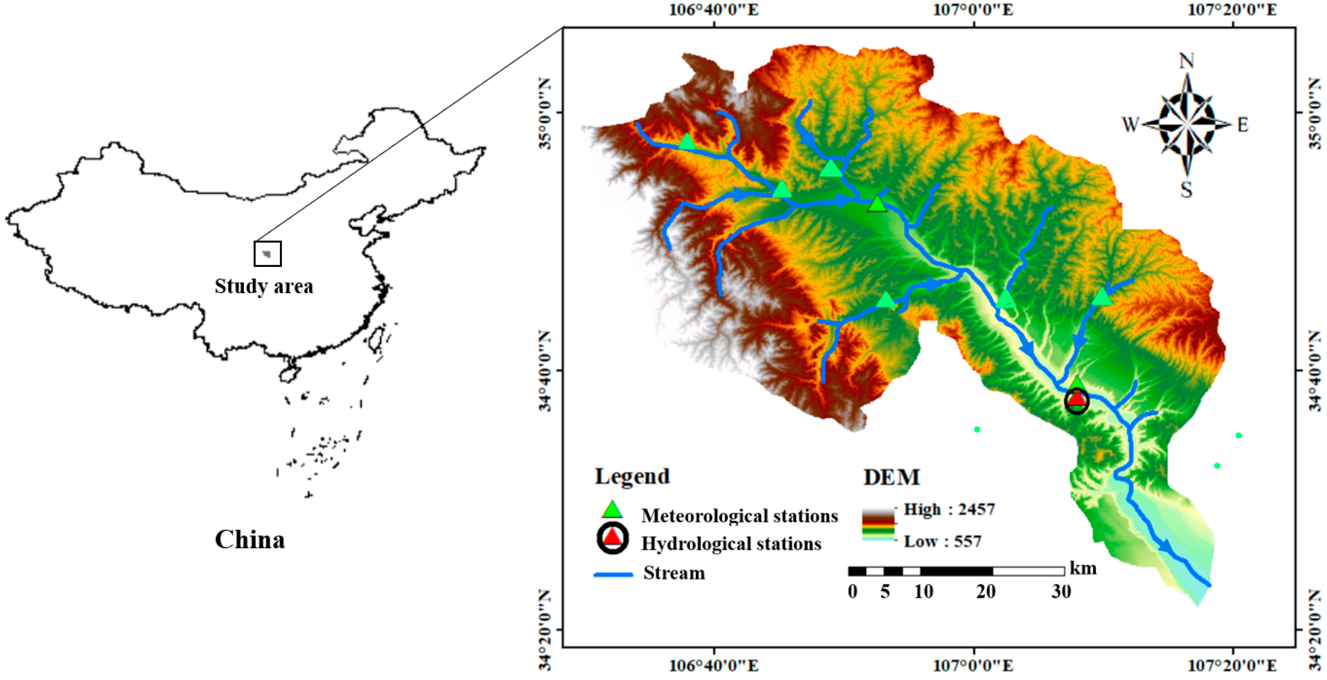
2.1. Regional Overview

Qianhe tributary is a watershed located north of the Weihe River Basin. It originates from the Shimiaoliang Mountain in the southern foot of Liupan Mountains in Gansu Province, flows through Huating County in Gansu Province and Longxian County, Qianyang, Fengxiang, and Didian Villages in Shaanxi Province, and merges into the Weihe River.

Qianhe tributary is located at 105°15′–107°15′ E and 34°20′–35°15′ N. The watershed is about 138 km wide and 50 km long, with an area of 3593 km², as shown in Figure 1. It is a semi-humid area and has an annual average temperature of 11.6 °C, an annual rainfall of 620.54 mm, an average runoff of 2.805 million m³·s⁻¹, and a runoff depth of 147.7 mm. The topography is diverse. The upper reaches are rocky mountainous areas with high vegetation coverage. The middle reaches are loess plateau areas with poor vegetation coverage. The lower reaches are loess plateau areas as well. The basin is dominated by plantation forests, economic forests, and grassland.

2.2. SWAT Model Construction

The SWAT model is a comprehensive model that can be used for physical process simulation and long-term simulation. It consists of three sub-models, i.e., hydrological process, pollution load, and soil erosion. The sub-model of hydrological process mainly focuses on runoff estimation and consists of two parts, namely, land calculation and river calculation. The basic hydrological response units (HRUs) of the model can be jointly defined by the regional parameters and the threshold. The model calculation process is as follows:

(1) The runoff components simulated in Swat’s runoff generation section include the slope surface runoff, soil flow, shallow groundwater runoff, and deep groundwater runoff. The runoff simulation can be calculated as:

$$s{w}_t=s{w}_0+{\displaystyle \sum _{i=1}^t\left(r_{day}-q_{surf}-e_a-w_{seep}-q_{gr}\right)}$$

(1)

where $s{w}_t$ is the final soil water content, $s{w}_0$ is the initial soil water content, $r_{day}$ is the daily precipitation, $q_{surf}$ is the daily surface runoff, $e_a$ is the daily evapotranspiration, $w_{seep}$ is the daily lateral infiltration flow and leakage amount of the soil profile, and $q_{gr}$ is the daily underground runoff.

(2) The surface runoff is calculated using the improved SCS curve number method as follows:

$$q_{surf}=\frac{{(r_{day}-l_0)}^2}{(r_{day}-l_0+S)}$$

(2)

where $l_0$ is the filled and trapped water, and $S$ is the intercepted water. The interception amount can be calculated using the following equation:

$$S=25.4(\frac{1000}{CN}-10)$$

(3)

where $CN$ is the coefficient of SCS, and the size of $CN$ is related to soil permeability, soil cover, and previous soil water content levels. The higher the $CN$ value, the smaller the intercepted water amount in the watershed, and the greater the surface runoff.

(3) In the traditional method, the intercepted water amount of the soil is the change in soil water content. In this paper, a modified interception method is introduced into the SWAT model, which is based on the cumulative evapotranspiration of plants.

$$q_{surfr}=(q_{surfr}^{\prime }-q_{surfr-1})·\left[1-\exp (-\frac{\mu }{t_{sc}})\right]$$

(4)

where $q_{surfr}$ is the daily runoff into the river, $r_{surfr}^{\prime }$ is the daily runoff on the slope, $r_{surfr-1}^{\prime }$ is the daily runoff intercepted on the slope in the sub-basin the day before, and $\mu$ is the coefficient of surface runoff stagnation. The larger the coefficient, the smaller the interception amount of water in the sub-basin. $t_{sc}$ is the time taken to form runoff at the sub-basin.

(4) The water that seeps into the soil can be obtained by subtracting the surface runoff from daily precipitation and further deducting the water that seeps out of the bottom layer of the soil. When the upper soil reaches complete saturation and the lower soil has not been saturated, the excess water will penetrate into the lower soil. The water transfer between the upper and lower soil layers can be calculated by the soil storage capacity as follows:

$$w_{s,i}=w{q}_{o,i}(1-\exp (\frac{-\mathsf{\Delta }t}{W{T}_i}))$$

(5)

where $w_{s,i}$ is the water seeping into the lower soil layer, $w{q}_{o,i}$ is the water that penetrates into the lower layer, and $W{T}_i$ is time for water motion.

The water that seeps out of the bottom soil layer enters the seepage zone and compensates for the underground aquifer, whereas due to differences in hydraulic conductivity and permeability between the upper and lower layers, once the permeability of the lower soil layer is smaller than that of the upper soil layer, the soil will be fully saturated by the trapped water, resulting in soil flow.

In the SWAT model of this study, runoff is assumed to only occur after the water content reaches the soil capacity and the portion of the maximum runoff is greater than that within the soil capacity. Then, the dynamic storage model (kinematic storage model) can be used to calculate the runoff in the soil by the following formula:

$$q_{\mathrm{int}}=0.024(\frac{2s{w}_{ex}·k·sl}{\mathrm{\Phi }·l_{hill}})$$

(6)

where $q_{\mathrm{int}}$ is the runoff in the slope soil, $s{w}_{gr}$ is the possible runoff in the soil layer of the slope, $k$ represents the conductivity of saturated water in the soil layer, $sl$ indicates the evaluated sub-basin slope, $\mathrm{\Phi }$ is the soil porosity, and $l_{hill}$ is the slope length.

Taking into account the hysteresis phenomenon of soil flow entering the river channel, after calculating the induced flow in the soil, the soil flow entering the river channel can be calculated using the following equation:

$$q_{\mathrm{int}t}=(q_0+q_{0-1})·[1-\exp (-\frac{1}{T{T}_{\mathrm{int}}})]$$

(7)

where $q_{\mathrm{int}t}$ represents the soil flow entering the river channel on that day, $q_0$ represents the runoff in the soil on the slope on that day, and $q_{0-1}$ represents the soil flow stored in the soil layer the day before that day. $T{T}_{\mathrm{int}}$ is the transfer time of soil flow.

(5) Groundwater runoff includes shallow groundwater runoff and deep groundwater runoff. Shallow groundwater runoff refers to water in the shallow saturated zone underground, which flows into the river runoff in the form of basic flow. Deep groundwater runoff refers to water in the confined saturated zone underground, which can be utilized for pumping irrigation. In underground runoff, only shallow groundwater has a capacity to compensate for river runoff in the basin. Assuming that the water level in the shallow saturated zone is higher than the given critical value, flow generates, and then the underground runoff can be calculated as:

$$q_{gr}=\{\begin{array}{l}{q}_{gr-1}·\exp (-{\beta }_{gr}·\mathsf{\Delta }t)+w_{swr}·[1-\exp (-{\beta }_{gr}·\mathsf{\Delta }t)],d{q}_{gr}\ge d{q}_{grb}\\ 0,d{q}_{gr}\le d{q}_{grb}\end{array}$$

(8)

where $q_{gr-1}$ is the shallow groundwater that entered the river the day before, ${\beta }_{gr}$ is the withdrawal coefficient of groundwater, $\mathsf{\Delta }t$ is the length of time, $w_{swr}$ is the amount of shallow groundwater compensation, $d{q}_{gr}$ is the shallow groundwater content, and $d{q}_{grb}$ is the critical shallow groundwater content.

(6) Generally, only vegetation evaporation is considered in SWAT runoff simulation. This study adds a term, soil evaporation. Specifically, both the vegetation evaporation and the soil evaporation at different depths were considered in the model simulation. The Penman Monteith method was used for vegetation evaporation calculation, which considers energy balance, water vapor diffusion theory, aerodynamics, and surface impedance. The equation is as follows:

$$E_P=\frac{\eta ·(h_{net}-\phi )+{\rho }_{air}·c_p·\frac{e_z^0-e_z{}_{}}{A_a}}{\mathrm{\Psi }·[\eta +\lambda ·(1+\frac{{\mathrm{A}}_v}{\mathrm{A}a})]}$$

(9)

$$E_{soil,h}=E_{msoil}^0\frac{h}{h+\exp (2.347-0.00713h)}$$

(10)

In Equation (9), $E_p$ indicates the evaporation ratio, $\eta$ represents the slope of the curve between saturated vapor and temperature, $h_{net}$ represents the net radiation, $\phi$ represents the soil heat flux, ${\rho }_{air}$ represents air density, $c_p$ represents the specific heat at a fixed pressure, $e_z^0$ represents the saturated water vapor at the Z height, $e_z$ represents the water vapor at the Z height, ${\mathrm{\Psi }}_v$ represents latent heat of evaporation, $\lambda$ is a hygrometer constant, $A_v$ is the vegetation canopy impedance, and $A_a$ is the dispersion impedance of the air layer.

In Equation (10), $E_{soil,z}$ is the water required for evaporation at depth $h$, $E_{soil,}^0$ is the maximum possible soil water evaporation, and $h$ represents the depth of the underground soil. It is worth noting that 50% of the water required for evaporation comes from the 10 mm soil surface, and 95% of the water required for evaporation comes from a soil depth of 0–100 mm.

The runoff calculation of the SWAT model was completed by the hydrological response calculation unit. The confluence calculation command was used to simulate the confluence of the reservoir, the superimposed command was used to compare the measured value with the simulated value, and the transfer command was used to transfer the water of a river section to other rivers.

2.3. Database and Hydrological Response Unit

The dataset used to establish a watershed hydrological simulation model includes DEM data, land use data, as well as data from the soil, meteorological, and hydrological databases.

The DEM data came from the geospatial data cloud ASTER GDEM (2005), with a resolution of 30 m. The slope, slope length, altitude, and watershed area of the sub-basin were extracted from the DEM data to generate a river network of the watershed, as shown in Figure 2.

The land use data were obtained from the Western China Environmental and Ecological Science Data Center, with a time range of 2000–2015 and a spatial resolution of 30 m. Land usage types in 2015 were reclassified to assigned values, as shown in Figure 2A. Land use types were divided into 8 categories, i.e., Cultivated land (CL) (including paddy fields and dry land), Woodland (WL) (including forestland, shrubland, clearing, and other forestland), Grassland (GL) (including high coverage grassland, medium coverage grassland, low coverage grassland), Waters (WT) (including canals, lakes, reservoirs, pits, and beaches), Residential area (RL) (urban land), Low-density residential area (RLL) (rural settlements), Transportation land (TL), and Wasteland and bare land (WAL).

The soil parameters in the study area, as shown in Figure 2B, came from the Chinese soil database. Soil parameters involved in the simulation include the following: depth from bottom to top of each soil layer (300 mm/1000 mm), wet soil density, effective water-bearing capacity of soil layer, soil organic carbon content, saturated water conductivity/saturated hydraulic conduction system, clay (diameter < 0.002 mm), loam soil (diameter 0.002–0.05 mm), sandy soil (diameter 0.05–2.0 mm), gravel (diameter > 2.0 mm), surface reflectance (0.01), soil erosivity factor, soil electrical conductivity, calcium carbonate content, soil PH.

Weather dataset includes daily precipitation, daily minimum temperature, daily maximum temperature, daily wind velocity, daily solar radiation, and daily relative moisture. These meteorological elements were obtained from a weather generator. Meteorological information came from independent observations at fixed weather stations. In this study, traditional Tyson polygon method, Kriging method, inverse distance method, and elevation correction method were combined to obtain the spatial interpolation for hydro-meteorological data.

For the sub-basin division, detailed watershed divisions and dense river networks are conducive to the formation of finer hydrological response units (HRUs). Therefore, under the premise of ensuring simulation accuracy, a suitable threshold should be set to improve the operating efficiency of the model. The Qianhe tributary was divided into 29 sub-basins, as shown in Figure 2C. In this study, the sub-basin was divided into 3 slope ranges, i.e., 0 to 1°, 1 to 10°, and above 10°, eventually generating 308 HRUs.

2.4. Parameter Sensitivity Evaluation

The parameter sensitivity test is a key step to calibrate and verify the model. SUFI-2 way was selected to conduct sensitivity test on the model parameters. In detail, we calculated the parameters generated from Latin hypercube random sampling and obtained the sensitivity ranking of the selected parameters.

In this study, we set 1 January 1970–31 December 1975 as the warm-up period, 1 January 1976–31 December 1990 as the calibration period, and 1 January 1991–31 December 2019 as the verification period. In the sensitivity analysis, 15 parameters were selected, i.e., SOL-ECC, CN2, V-ECC, SOL-AHC, SOL-AW, MSF-RC, BF-C, BAN-BRC, GRO-RC, REVAPMN-C, SUR-RC, SM-C, STMI-C, BOI-MEF, and T-DR, as shown in

Table 1. Parameter sensitivity test result.

Parameter	Definition	S	p	Order
BF-C	Base flow coefficient	7.4890	0.0035	1
SOL-AW	Soil available water capacity	6.1902	0.0735	2
CN2	Runoff curve coefficient	9.3272	0.0002	3
SOL-ECC	Soil evaporation compensation coefficient	5.1393	0.1377	4
BAN-BRC	Base flow coefficient of bank regulated storage	0.6197	0.5349	5
MSF-RC	Manning slope flow coefficient	4.3573	0.1952	6
GRO-RC	Shallow groundwater runoff coefficient	0.6973	0.5931	7
SOL-AHC	Soil conductivity of saturated water	5.7720	0.0739	8
V-ECC	Vegetation evapotranspiration compensation coefficient	2.9348	0.3571	9
REVAPMN-C	Re-evaporation coefficient of shallow aquifer	0.5438	0.6393	10
SUR-RC	Surface runoff lag coefficient	0.4981	0.7126	11
SM-C	Maximum snowmelt coefficient	0.3362	0.7593	12
STMI-C	Minimum temperature for snowmelt	0.2461	0.8913	13
BOI-MEF	Biological mixing efficiency factor	0.0737	0.9251	14
T-DR	Temperature drop rate	0.0259	0.9481	15

.

The S value and p value were used to evaluate the parameter sensitivity. The S value indicates the parameter sensitivity, and the p value indicates the significance. Three iterations of 500 simulations were periodically performed on the model parameters until we obtained the ideal parameter sensitivity analysis and calibration results. Finally, the top 9 parameters in terms of sensitivity for the Qianhe tributary were determined, as listed in

Table 2. Parameter calibration result.

Parameter	Ranges	Optimal Value	Sensitivity Order
BF-C	0–1	0.4733	1
SOL-AW	0–1	0.6495	2
CN2	20–50	39.3275	3
SOL-ECC	0–1	0.5543	4
BAN-BRC	0–1	0.36487	5
MSF-RC	0–0.5	0.039	6
GRO-RC	100–1000	649.402	7
SOL-AHC	10–500	41.43783	8
V-ECC	0–1	0.27392	9

. The most sensitive parameters were BF-C, SOL-AW, CN2, SOL-ECC, and BAN-BRC, successively.

Three different measures were used to evaluate the model parameters, including coefficient of Nash–Sutcliffe efficiency (NSE), decisive coefficient (R), and relative error (RE).

3. Results and Discussion

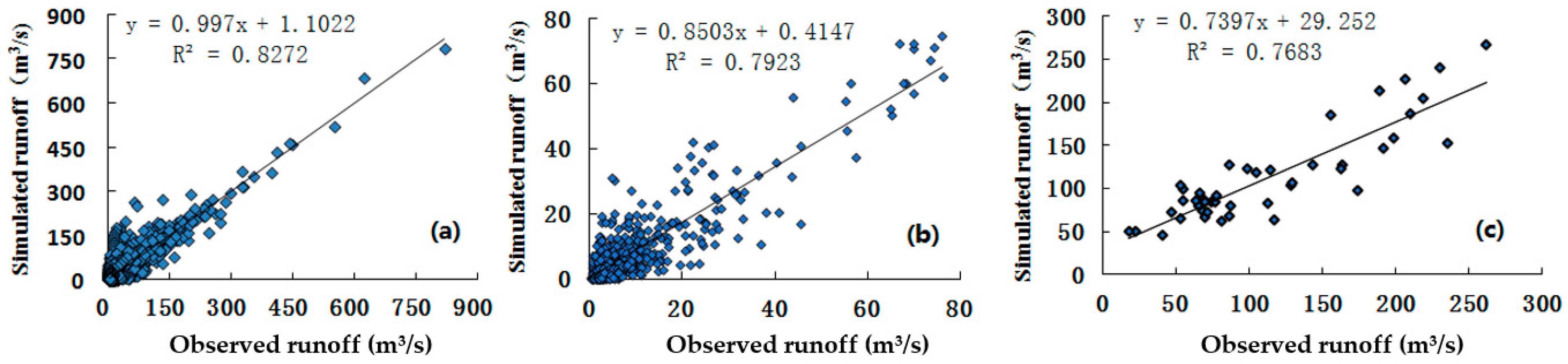
3.1. Runoff Simulation Evaluation

We took the phase of 1976–1990 as the calibration period and the phase of 1991–2019 as the verification period. The optimal parameters of calibration were brought into the SWAT model to simulate the daily, monthly, and annual runoff. The daily data, as shown in Figure 3, were applied to simulate the runoff under land use changes in 2015.

Figure 3 shows that most of the simulated daily runoff values are smaller than the measured values in the calibration period from 1976 to 1990, while most of the simulated values are larger than the measured values in the validation period from 1991 to 2019. Moreover, when the runoff is at a high value, the error between the measured value and the simulated value is smaller at the range of 2.58–9.52%, and at a low value of runoff, the error is more than 15%. This indicates that the simulation error is related to the amount of runoff. When the runoff was measured as below as 0.3–15 m³/s, the simulated value was higher than the measured value with a large error of 15–36%. When the measured runoff was between 40 and 100 m³/s, the error was 10–18%. When the measured runoff was above 100 m³/s, the simulated value was smaller than the measured value. The relative error was less than 9.8%, which was within the test reliability range.

Figure 4 shows that the simulated values of runoff in December, January, February, and Spring and Autumn are slightly higher than the measured values during the validation period from 1991 to 2019, while the simulated values of runoff from July to September are lower than the measured values. The difference between the simulated value and the measured value in the calibration period is 0.34 m³/s and 0.13 m³/s, while the difference in the validation period is 0.24 m³/s and −0.36 m³/s, respectively. The simulated monthly runoff in the calibration period is larger than that in the validation period.

Figure 4 shows that in the summer flood season, the precipitation is more sufficient, and the simulated runoff reaches a higher value, while in winter, the precipitation is less and the simulated runoff is at a low value. When the measured monthly runoff is 15–69.8 m³/s, the simulated monthly runoff is underestimated, and the relative error is 4.5%. When the measured monthly runoff is below 3 m³/s, the simulated values are higher, and the error is between 20 and 35%. On the whole, the simulation effect in the period of a large runoff is better than that in the low-runoff period, and the simulated value is higher than the measured value. In summer, the maximum/minimum values of the simulated runoff are consistent with the measured runoff, and the annual/monthly/daily measured runoff has a positive correlation with the simulated runoff. At the calibration period, the simulated value is slightly higher than the measured value, while at the verification period, the simulated value is lower than the measured value. Overall, the simulation error in the dry period (winter) is relatively large but relatively small in the rainy period (summer). The simulated monthly/daily runoff is consistent with the change in measured precipitation, with an overestimation in the peak value of the simulated runoff. The peak and valley values of annual runoff are well simulated (Figure 5), whereas the annual runoff reaches a high value in 1983 and 1989 but a low value in 1987; among the three years, the errors of annual runoff between measurement and simulations are relatively large. Taken together, the annual runoff is overestimated, and the relative errors vary due to different runoff sizes. When the measured annual runoff is between 0.4 and 4.0 m³/s, the relative error is 10–35%; when the measured annual runoff is between 4.1 and 13.5 m³/s, the relative error is less than 5.3%. Generally, the relative error in the high-value annual runoff simulations is small but large in the low-value runoff simulations; only the annual runoff in 1981, 1991, 1992, and 1998 are underestimated.

From Figure 6, it can be seen that the correlations between simulated values and measured values are significant. The evaluation coefficients of NSE, R, and RE are within the allowable range, which are 0.82–0.86, 0.76–0.83, and 3.06–10.08%, respectively. The evaluation coefficient indicates that the model is suitable for monthly runoff simulations. An uncertainty test was also executed by automatic P in the SWAT model, and the simulated value was lower than the 95% prediction uncertainty threshold, indicating that the uncertainty is low. Although the simulated value is lower or higher than the measurement in several years, the overall simulation error is within the allowable range. On the whole, when the annual, monthly, and daily runoff is 4–13.5 m³/s, 4–69.8 m³/s, and 40–189.3 m³/s, respectively, the relative error is smaller and the simulation effect is better. Among the three time scales of the runoff simulations, the daily runoff simulation shows the best performance, followed by the monthly simulation, and, finally, the annual simulation.

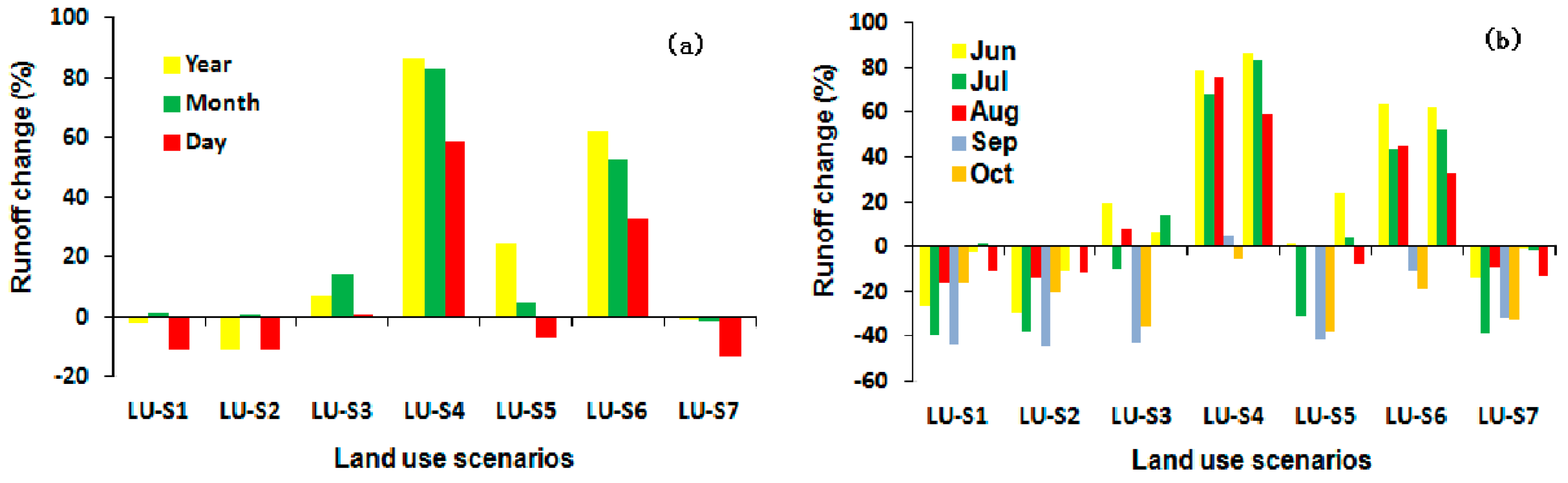
3.2. Runoff Simulation under Land Use Changes

There are various commonly used methods for analyzing land use change scenarios [40]. Given the limitations of data and technology, this study adopted the extreme assumption method regarding land use change scenarios, which converts all one land use types or more land use types into another land use type. This method can intuitively demonstrate the impact of changes in specific land use types on runoff. The extreme assumption method was used to set up the land use change scenarios to simulate runoff. As there have been very few land use changes since 2015, the year 2015 was chosen as the base year for future simulation and comparison. Taking into account the impact of land use change on runoff under the influence of human activities, seven land use change scenarios were assumed based on 2015 (

Table 3. Actual land use types of the Qianhe tributary and the specific areas under the seven land use change assumption scenarios (hm²).

Land Use Type	Land Use Change Scenario
	LU-T1	LU-T2	LU-T3	LU-T4	LU-T5	LU-T6	LU-T7
Cultivated land	0	0	3086	0	0	0	1216
Woodland	1956	743	0	0	743	743	743
Grassland	1130	2343	0	0	1130	1130	1130
Waters	62	62	62	62	62	62	62
Residential area	4	4	4	4	1217	4	4
Low-density residential area	45	45	45	45	45	45	45
Transport land	17	17	17	17	17	1230	17
Wasteland, bare land	3	3	3	3089	3	3	0

), and the specifics are as follows: LU-S1, all cultivated lands and wastelands are converted to forest land, and other land types remain unchanged; LU-S2, following the idea of returning a farmland to grassland, all cultivated lands and wastelands are converted to grassland; LU-S3, all woodlands and grasslands are converted to arable land, and other land use types remain unchanged; LU-S4, due to the deterioration of land structure, all cultivated lands, forest lands, and grasslands have been degraded into wasteland, and other land use types remain unchanged. LU-S5, all cultivated lands are converted to residential areas, and other land use types remain unchanged; LU-S6, all cultivated lands are converted to transportation land, and other land use types remain unchanged. LU-S7, all wastelands are converted to grassland, and other land use types remain unchanged.

Figure 7 shows the comparison of monthly and annual runoffs between simulations and measurements under different land use change scenarios. It can be seen that the runoff under LU-S4 and LU-S6 scenarios is the largest, significantly larger than that in the base year. The simulated runoff in other scenarios is relatively small. Compared with the average runoff under the 2015 land use scenario, the runoff under the land use change scenarios of LU-S3 to LU-S6 increases significantly, increasing by 5.2–54.6% and 8.4–93.2% corresponding to the annual and monthly runoffs, respectively. The runoff of LU-S4 and LU-S6 increases the most, with the largest annual increase being 75.1% and 54.5%, and the largest monthly increase being 93.2% and 64.1%, respectively. In contrast, the annual runoff under other land use change scenarios decreases by less than 24.6%, and the monthly runoff decreases by less than 6.8%. The runoff trend is the same from June to October during the flood season, and the runoff change is large from July to September. Figure 8 shows the maximum runoff change under land use change scenarios. The maximum runoff of LU-S4 and LU-S6 increases by 62% and 52%, respectively, and the runoff of LU-S7 decrease by up to 37%. It can be seen that in the monthly runoff simulation, the increase in cultivated land, forest land, and grassland has a small weakening effect on the runoff, while the wasteland still has a significant influence. The difference in runoff between the abundance period and drought period is increased, and the seasonal change is more obvious.

The land use types under the LU-S1 and LU-S2 scenarios are mainly woodland and grassland. Since the surface vegetation has the functions of absorption, interception, and transpiration of precipitation, runoff is reduced, but the degree of impact is relatively small. Under the LU-S4 scenario, the more arable land results in the reduction of surface runoff. However, there is no vegetation on the surface under the LU-S4 scenario, and the interception effect on runoff is greatly reduced, thus increasing the total amount of surface runoff under this scenario and exacerbating soil erosion. Under the LU-S6 scenario, when all cultivated lands are converted into transportation land, surface runoff increases greatly. Due to the small area of the wasteland, the interception of precipitation is affected. This indicates that the interception and transpiration of precipitation by vegetation coverage are important factors affecting the surface runoff.

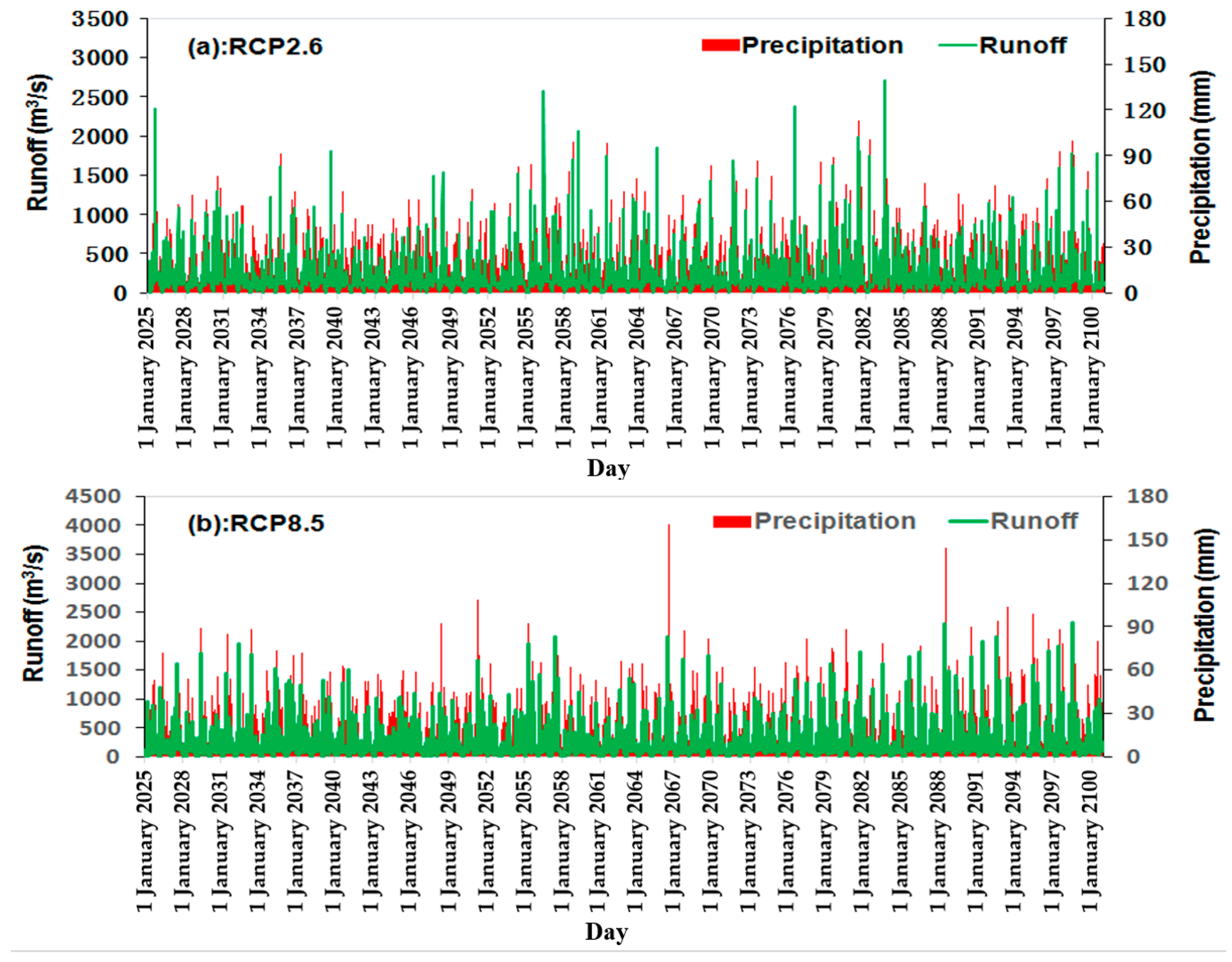
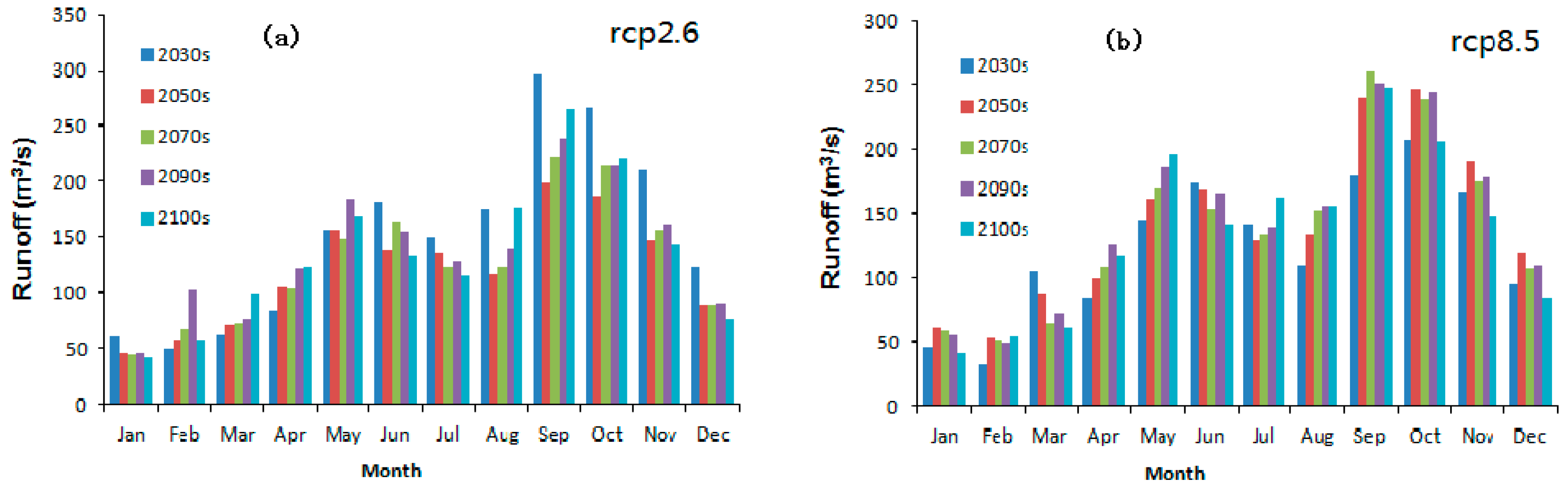
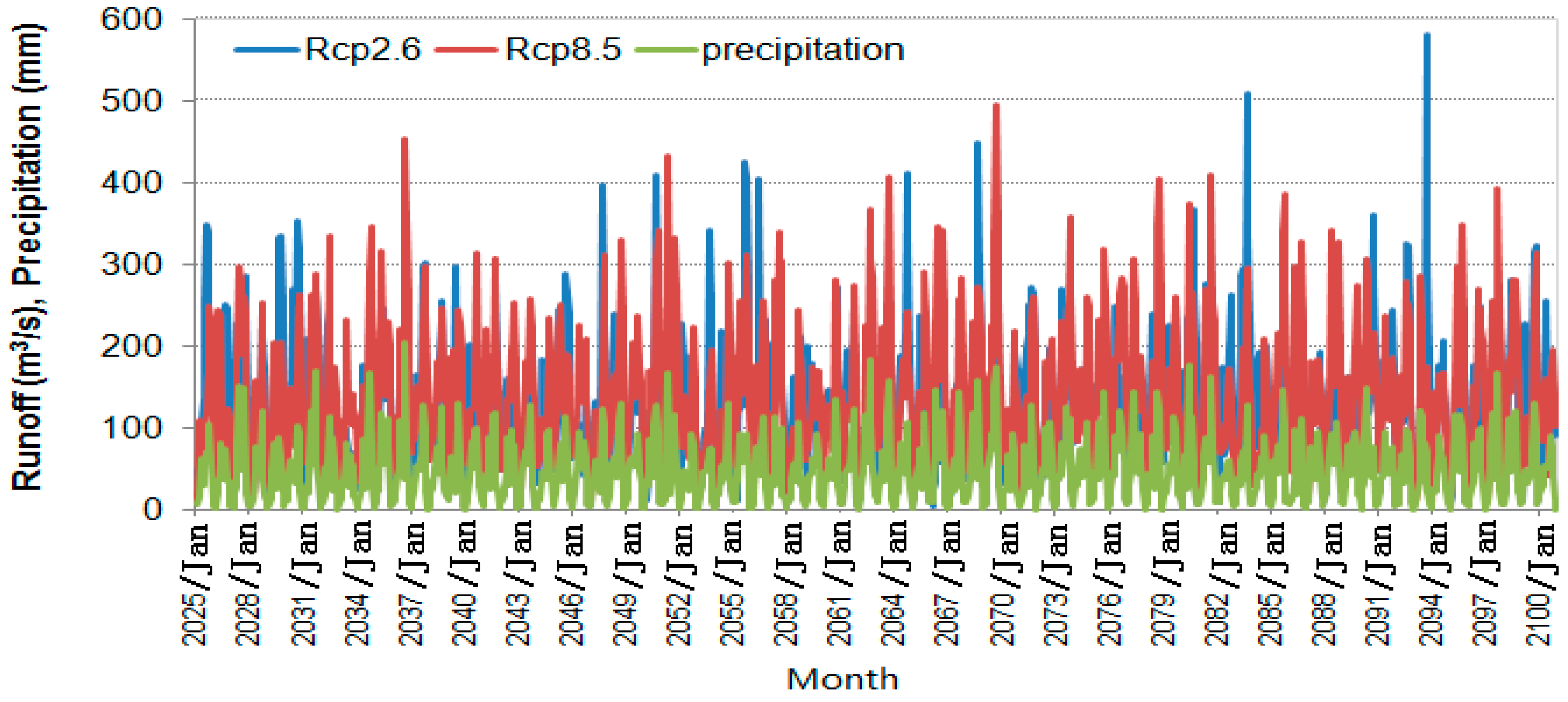
3.3. Runoff Response to Climate

In order to further analyze the relationship between climate factors and runoff, correlation analysis and wavelet cross sweep were used to analyze the relationship between runoff, precipitation, and temperature (Figure 9). It can be seen from Figure 9 that precipitation shows a positive correlation with runoff, and the resonance energies during the 2–4 year and 8-year cycles are relatively large. The relationship between temperature and runoff is mainly reflected in the significant cross resonance energy for periods after 2000, which are 2–3 years and 6–8 years. This indicates that precipitation and temperature have important influence on runoff. Therefore, different precipitation and temperature climate scenarios were set during annual and monthly runoff simulations. In comparison with the measured runoff, the impact degree of temperature and precipitation on runoff simulation was clarified using the SWAT model.

Further, we made assumptions as follows: the temperature remains unchanged or changes around ±2 °C, ±1 °C, and the precipitation remains unchanged or changes around ±10%, ±25%. Then, 24 permutations and combinations of climate scenarios were designed, as listed in

Table 4. Climate change assumption scenarios.

Temperature Change	Precipitation Change
	−25%	−10%	0	+10%	+25%
−2 °C	C-S1	C-S2	C-S3	C-S4	C-S5
−1 °C	C-S6	C-S7	C-S8	C-S9	C-S10
0	C-S11	C-S12	C-S0	C-S13	C-S14
+1 °C	C-S15	C-S16	C-S17	C-S18	C-S19
+2 °C	C-S20	C-S21	C-S22	C-S23	C-S24

. The simulation results are shown in Figure 10. Among them, the C-S0 scenario is the measured temperature, precipitation, and runoff. In the C-S5 scenario where the temperature decreases by 2 °C and precipitation increases by 25%, the average annual runoff is the largest, increasing by 1.3 times than that in the C-S0. However, in the C-S20 scenario where the temperature increases by 2 °C and precipitation decreases by 25%, the average annual simulated runoff decreases by 67.5%. When the temperature remains unchanged and precipitation decreases or increases by 10%, the annual runoff decreases by 35.93% or increases by 41.49%, while the monthly runoff decreases by 34.42% or increases by 39.95%. However, when the precipitation remains unchanged and temperature increases or decreases by 1 °C, the runoff decreases by −0.72% or increases by 5.91%, while the monthly runoff decreases by 0.04% or increases by 5.7%. From the simulation results of monthly runoff, it can be seen that under the C-S5 scenario, the surface monthly runoff reaches its maximum value, increasing by 1.29 times, while under the CS-20 scenario, the monthly runoff is the smallest, decreasing by 64.5%. This indicates that runoff is more significantly affected by temperature rise and precipitation decline. The simulated scenario is consistent with the variation trend of the measured runoff, but the magnitude of variation of the simulated runoff differs for each scenario.

Regarding the simulation of regional climate impact, many downscaling means have been exploited to resolve the shortcomings of the GCM climate scenario by enhancing the spatial resolution. In this study, statistical downscaling was performed by establishing the relationship between the meteorological data of the forecast station and atmospheric circulation factors based on station observation data and NCEP reanalysis data. Local climate is based on large-scale climate, and within a given range, there should be a correlation between large-scale and small-scale climate variables. By establishing an empirical correlation between large-scale climate elements (prediction factors) and local climate elements (predicted quantities), and then applying this empirical correlation to the output of regional models, corresponding information for any location can be obtained.

There are more than 20 climate models. Referring to reference [40], the input model, HadCM3 from CMIP6 (Resolution of 0.25° × 0.25°), was considered more suitable and outperformed other models for downscale simulation in this region. Therefore, the GA model climate scenario product was used for future-runoff simulation. Under the climate scenarios of RCP8.5 and RCP2.6, the daily output data of HadCM3 from CMIP6 during 2025 to 2100 were used as input data of the SWAT model to simulate changes in precipitation and temperature in the watershed, and then future runoff simulation predictions were conducted based on simulated meteorological elements. Figure 11, Figure 12, Figure 13 and Figure 14 show the change in daily runoff, monthly runoff, and annual runoff in the future. It can be seen that the precipitation change fluctuates due to the precipitation change caused by many factors, leading to runoff fluctuations. On the whole, the simulated runoff under the low-emission RCP2.6 scenario is greater than that under the high-emission RCP8.5 scenario, indicating that the runoff would be reduced in a high-emission scenario. The runoff is projected to be significantly reduced in 2040, 2060, and 2080, and the runoff reduction under the high-emission RCP8.5 scenario is more significant than that under the low-emission RCP2.6 scenario. The maximum annual runoff greater than 180 m³·s⁻¹ is reduced by an average reduction of 20.3% and 22.7% under the RCP2.6 and RCP8.5 climate scenarios. According to the simulation, the maximum runoff of 2030, 2060, 2080, and 2090 is relatively large, and the possibility of causing a flood is also increased.

3.4. Discussion

The above simulation results showed that the top nine sensitivity parameters after calibration can well simulate the runoff of the Qianhe tributary. The simulation results were basically consistent with the existing findings [41]. In addition, the simulated peak runoff during the flood season was overestimated, the changes in simulated runoff were consistent with the precipitation change, and the research results were basically consistent with the simulation results in the literature [42]. Sensitivity analysis results showed that BF-C, SOL-AW, and CN2 were the most important parameter in the runoff simulation of the Qianhe tributary, which was different from previously reported results [43]. The inconsistency might be due to the influence of soil and land use changes in different basins. The evaluation of simulation parameters showed that the error in the verification period was relatively large but was relatively small in the calibration period, indicating certain uncertainties in the simulation process, whereas the errors in both the verification period and the calibration period were within the acceptable range.

In addition, the simulated value in the rainy season was greater but was low in the dry season. Due to the different runoff data at the annual, monthly, and daily time-scales, there were differences in simulation errors. The time series length of daily runoff contained 10,591 samples, with 348 samples per month and only 29 samples per year, which minimized the error in daily runoff, followed by the monthly samples and, finally, the annual samples. The longer the time series of runoff samples, the better the simulation effect. Previous studies have found that DEM resolution has an impact on runoff simulation [44]. The phenomenon of the measured value being smaller than the simulated value might be caused by the influence of the watershed area unit. Research has shown that the calculated runoff through the SCS curve could be affected by the DEM resolution [45], and the slope is the most sensitive parameter. Moreover, the SWAT model has been proven to be able to achieve a good simulation effect in large-scale watershed runoff simulation and management decision-making [46]. And in this study, the SWAT hydrological model also demonstrated a good simulation effect in the small watershed area, which divided the watershed into smaller basic units to improve the simulation accuracy.

However, the model also has shortcomings. In large-scale simulations, if the sub-basin area is large and the spatial difference of precipitation is significant as well, there will be large errors in the simulation results. As we know, all grasslands and woodlands in the watershed have the same slope. Previous research has indicated that grassland is usually located in valleys, while woodland is located in a steeper area than grassland. If the different land use types in a watershed exhibit different characteristics, the simulation error will be larger [47]. In addition, the land use types of smaller areas in the simulation, such as untreated roads, bare land, and construction land, are usually not considered but attributed to other land types. However, these smaller areas may yield more sand than the same area of grassland. In the future, temperature rise and precipitation reduction will exacerbate runoff reduction. Therefore, the impact of temperature and precipitation on runoff is a complex process, and the mutual physical mechanism needs further discussion.

4. Conclusions

The SWAT hydrological model established in this study showed a good effect on the runoff simulation of the Qianhe tributary. Through a parameter sensitivity analysis, we found that in the semi-arid area, the river runoff is mainly compensated for by precipitation. The top nine parameters that are very sensitive to the runoff simulation were determined. Typically, BF-C, SOL-AW, and CN2 had the highest sensitivity. The daily runoff simulation showed the best performance, followed by the monthly runoff simulation, and then the annual runoff simulation. The simulated runoff with a low value was overestimated.

The simulations under land use change scenarios showed that the cultivated land, grassland, and forest land had a negative effect on runoff, while wasteland and transportation land had a positive effect on runoff. In particular, when woodland, cultivated land, and grassland became wasteland, the runoff change was greater during the flood season. The interception and transpiration of runoff by vegetation coverage were important factors affecting the surface runoff. The runoff was more significantly affected by temperature rise and precipitation decrease, and the variation magnitude of the simulated runoff differed for each scenario.

In the simulation of the future, the simulated runoff under the assumed climate scenarios of RCP8.5 and RCP2.6 showed a decline in different degrees. Due to the influence of various factors, precipitation decrease/increase in different decades would result in runoff reduction or an increase in the possibility of flooding in different years. The maximum runoff of 2030, 2060, 2080, and 2090 would be relatively large, and the possibility of causing a flood would increase.

The SWAT model assumes that each HRU exhibits the same characteristics. Therefore, when conducting SWAT simulation in different watersheds, more attention should be paid to the determination of the sensitivity of model parameters, the nonlinear relationship between hydrological response (output), and hydrological characteristics (input), as well as the scale effect of the model.

References

1. Danneberg, J. Changes in runoff time series in Thuringia, Germany–Mann-Kendalltrend test and extreme value analysis. Adv. Geosci. 2012, 31, 49–56. [Google Scholar] [CrossRef]
2. Liu, Y.G.; Yu, K.K.; Zhao, Y.Q.; Bao, J.C. Impacts of Climatic Variation and Human Activity on Runoff in Western China. Sustainability 2022, 14, 942. [Google Scholar] [CrossRef]
3. Liu, Y.; Wen, Y.; Zhao, Y.; Hu, H. Analysis of Drought and Flood Variations on a 200-Year Scale Based on Historical Environmental Information in Western China. Int. J. Environ. Res. Public Health 2022, 19, 2771. [Google Scholar] [CrossRef]
4. Sun, T.; Yang, Y.-M.; Wang, Z.-G.; Yong, Z.-W.; Xiong, J.-N.; Ma, G.-L.; Li, J.; Liu, A. Spatiotemporal variation of ecological environment quality and extreme climate drivers on the Qinghai-Tibetan Plateau. J. Mt. Sci. 2023, 20, 2282–2297. [Google Scholar] [CrossRef]
5. Cinto Mejía, E.; Wetzel, W.C. The ecological consequences of the timing of extreme climate events. J. Ecol. Evol. 2023, 13, e9661. [Google Scholar] [CrossRef]
6. Liu, Y.G.; Wang, N.L.; Wang, L.G.; Zhao, Y.Q.; BoWu, X. Application of GIS in regional ecological risk assessment of water resources. Environ. Eng. Manag. J. 2013, 12, 1465–1474. [Google Scholar] [CrossRef]
7. Liu, Y.G.; Zhang, J.H.; Zhao, Y.Q. The Risk Assessment of River Water Pollution Based on a Modified Non-Linear Model. Water 2018, 10, 362. [Google Scholar] [CrossRef]
8. Li, Z.; Shao, Q.; Xu, Z.; Xu, C. Uncertainty issues of a conceptual water balance model for a semi-arid watershed in northwest China. Hydrol. Process. 2013, 27, 304–312. [Google Scholar] [CrossRef]
9. Huang, S.; Huang, Q.; Chen, Y. Quantitative estimation on contributions of climate changes and human activities to decreasing runoff in Weihe River Basin, China. Chin. Geogr. Sci. 2015, 25, 569–581. [Google Scholar] [CrossRef]
10. Zhang, P.; Liu, R.; Bao, Y.; Wang, J.; Yu, W.; Shen, Z. Uncertainty of SWAT model atdifferent DEM resolutions in a large mountainous watershed. Water Res. 2014, 53, 132–144. [Google Scholar] [CrossRef]
11. Forsythe, N.; Fowler, H.; Blenkinsop, S.; Burton, A.; Kilsby, C.; Archer, D.; Harpham, C.; Hashmi, M. Application of a stochastic weather generator to assess climate change impacts in a semi-arid climate: The Upper Indus basin. J. Hydrol. 2014, 517, 1019–1034. [Google Scholar] [CrossRef]
12. Hao, Z.C.; Xie, H.H.; Huang, G.R.; Qin, J.; Jie, H. Spatial Scale Analysis of the TOPMODEL Model. J. Glaciol. Geocryol. 2010, 32, 587–592. [Google Scholar]
13. Xin, X.; Tian, Q.A.; Xiao, D.L. Application of a Fractional Instantaneous Unit Hydrograph in the TOPMODEL: A Case Study in Chengcun Basin, China. Appl. Sci. 2023, 13, 2245. [Google Scholar]
14. Ni, A.Q.; Jun, Y.Z.; Xu, G.W.; Cui, J.; Song, Y.-X.; Sun, X.-Y. A modified TOPMODEL introducing the bedrock surface topographic index in Huangbengliu watershed, China. J. Mt. Sci. 2022, 19, 3517–3532. [Google Scholar]
15. Yi, X.; Shu, S.P.; Agnès, D.; Ciais, P.; Gumbricht, T.; Jimenez, C.; Poulter, B.; Prigent, C.; Qiu, C.; Saunois, M. Author Correction: Gridded maps of wetlands dynamics over mid-low latitudes for 1980–2020 based on TOPMODEL. Sci. Data 2022, 9, 3517–3532. [Google Scholar]
16. Farid, B.; Hadi, M.F.; Touraj, S.; Haghighi, A.T.; Talebi, A. Spatial–temporal analysis of landslides in complex hillslopes of catchments using Dynamic Topmodel. Acta Geophys. 2022, 70, 1417–1432. [Google Scholar]
17. Kazmi, D.H.; Li, J.; Rasul, G.; Tong, J. Statistical downscaling and future scenario generation of temperatures for Pakistan region. J. Theor. Appl. Climatol. 2015, 120, 341–350. [Google Scholar] [CrossRef]
18. Liu, Z.; Martina, M.L.V.; Todini, E. Flood forecasting using a fully distributed model: Application of the TOPKAPI model to the Upper Xixian Catchment. Hydrol. Earth Syst. Sci. 2005, 9, 347–364. [Google Scholar] [CrossRef]
19. Deng, P.; Li, Z.J.; Liu, Z.Y. Numerical algorithm of distributed TOPKAPI model and its application. Water Sci. Eng. 2008, 1, 14–21. [Google Scholar] [CrossRef]
20. Iqra, A.; Javed, I.; Li, J.S. Modeling Hydrological Response to Climate Change in a Data-Scarce Glacierized High Mountain Astore Basin Using a Fully Distributed TOPKAPI Model. Climate 2019, 7, 127. [Google Scholar]
21. Ragettli, S.; Pellicciotti, F. Calibration of a physically based, spatially distributed hydrological model in a glacierized basin: On the use of knowledge from glaciometeorological processes to constrain model parameters. Water Resour. Res. 2012, 48. [Google Scholar] [CrossRef]
22. Hengade, N.; Eldho, T. Assessment of LULC and climate change on the hydrology of Ashti Catchment, India using VIC model. J. Earth Syst. Sci. 2016, 125, 1623–1634. [Google Scholar] [CrossRef]
23. Diwan Mohaideen, M.M.; Varija, K. Improved vegetation parameterization for hydrological model and assessment of land cover change impacts on flow regime of the Upper Bhima basin, India. J. Acta Geophys. 2018, 66, 697–715. [Google Scholar] [CrossRef]
24. Hengade, N.; Eldho, T.I.; Ghosh, S. Climate change impact assessment of a river basin using CMIP5 climate models and the VIC hydrological model. J. Hydrol. Sci. J. 2018, 89, 596–614. [Google Scholar] [CrossRef]
25. Lilhare, R.; Déry, S.J.; Stadnyk, T.A.; Pokorny, S.; Koenig, K.A. Warming soil temperature and increasing baseflow in response to recent and potential future climate change across northern Manitoba, Canada. Hydrol. Process. 2022, 36, e14748. [Google Scholar] [CrossRef]
26. Carvalho, V.S.O.; da Cunha, Z.A.; Alvarenga, L.A.; Beskow, S.; de Mello, C.R.; Martins, M.A.; de Oliveira, C.d.M.M. Assessment of land use changes in the Verde River basin using two hydrological models. J. S. Am. Earth Sci. 2022, 118, 103954. [Google Scholar] [CrossRef]
27. Zhou, Q.; Chen, L.; Singh, V.P.; Zhou, J.; Chen, X.; Xiong, L. Rainfall-runoff simulation in karst dominated areas based on a coupled conceptual hydrological model. J. Hydrol. 2019, 471, 524–533. [Google Scholar] [CrossRef]
28. Hiep, N.H.; Luong, N.D.; Nga, T.T.V.; Hieu, B.T.; Ha, U.T.T.; Du Duong, B.; Long, V.D.; Hossain, F.; Lee, H. Hydrological model using ground- and satellite-based data for river flow simulation towards supporting water resource management in the Red River Basin, Vietnam. J. Environ. Manag. 2018, 80, 346–355. [Google Scholar] [CrossRef]
29. Lee, H.E.; Shim, S.; Choi, Y.; Bae, Y.S. NADPH oxidase inhibitor development for diabetic nephropathy through water tank model. Kidney Res. Clin. Pract. 2022, 41, S89–S98. [Google Scholar] [CrossRef]
30. Guang, S.L.; Toraharu, W.; Takeshi, S. Two-phase Flow Analysis for Small-scale Ballast Water Tank Model by Hydraulics Experiment and Simulations. IOP Conf. Ser. Earth Environ. Sci. 2022, 972, 012048. [Google Scholar]
31. Shi, X.L.; Li, Y.; Yang, Z.Y. Response of runoff on land use/cover change in Nuomin river basin based on SWAT model. J. Water Resour. Water Eng. 2016, 27, 65–69. [Google Scholar] [CrossRef]
32. Liu, Y.; Wang, N.; Zhang, J.; Wang, L. Climate change and its impacts on mountain glaciers during 1960–2017 in western China. J. Arid. Land 2019, 11, 537–550. [Google Scholar] [CrossRef]
33. Chen, X.L.; Huang, G.R. Runoff simulation of Feilaixia watershed of Beijiang River based on SWAT Mod. J. Water Resour. Water Eng. 2017, 28, 1–7. [Google Scholar]
34. Rahman, K.; Maringant, C.; Beniston, M.; Widmer, F.; Abbaspour, K.; Lehmann, A. Streamflow Modeling in a Highly Managed Mountainous Glacier Watershed Using SWAT: The Upper Rhone River Watershed Case in Switzerland. Water Resour. Manag. 2013, 27, 323–339. [Google Scholar] [CrossRef]
35. Akansha, K.; Manoj, K.J. Hydrological Simulation in a Forest Dominated Watershed in Himalayan Region Using SWAT Model. Water Resour. Manag. 2013, 27, 3005–3023. [Google Scholar]
36. Anaba, L.A.; Banadda, N.; Kiggundu, N.; Wanyama, J.; Engel, B.; Moriasi, D. Application of SWAT to assess the effects of land use change in the Murchison Bay Catchment in Uganda. Comput. J. Water Energy Environ. Eng. 2017, 6, 24–40. [Google Scholar]
37. Ze, P.Z.; Qing, Z.W.; Qing, Y.G.; Xiao, X.; Mi, J.; Lv, S. Research on the optimal allocation of agricultural water and soil resources in the Heihe River Basin based on SWAT and intelligent optimization. Agric. Water Manag. 2023, 279, 108177. [Google Scholar]
38. Mendonça, F.S.D.; Natália, P.S.D.; Proença, R.O.D.; Di Lollo, J.A. Using the SWAT model to identify erosion prone areas and to estimate soil loss and sediment transport in Mogi Guaçu River basin in Sao Paulo State, Brazil. Catena 2023, 222, 106872. [Google Scholar]
39. Verma, K.S.; Prasad, D.A.; Verma, K.M. An Assessment of Ongoing Developments in Water Resources Management Incorporating SWAT Model: Overview and Perspectives. Nat. Environ. Pollut. Technol. 2022, 21, 1963–1970. [Google Scholar] [CrossRef]
40. Liu, Y.; Xu, Y.; Zhao, Y.; Long, Y. Using SWAT Model to Assess the Impacts of Land Use and Climate Changes on Flood in the Upper Weihe River, China. Water 2022, 14, 2098. [Google Scholar] [CrossRef]
41. Manoj, J. SWAT: Model use, calibration, and validation. Environ. Sci. Geosci. 2012, 55, 1491–1508. [Google Scholar] [CrossRef]
42. Wu, H.J.; Chen, B. Evaluating uncertainty estimates in distributed hydrological modeling for the Wenjing River watershed in China by GLUE, SUFI-2, and ParaSolmethods. Ecol. Eng. 2015, 76, 110–121. [Google Scholar] [CrossRef]
43. Lu, Z.; Zou, S.; Xiao, H.; Zheng, C.; Yin, Z.; Wang, W. Comprehensive hydrologic calibration of SWAT and water balance analysis in mountainous watersheds in northwest China. J. Phys. Chem. Earth A/B/C 2015, 56, 79–82. [Google Scholar] [CrossRef]
44. Yesuf, H.M.; Melesse, A.M.; Zeleke, G.; Alamirew, T. Streamflow prediction uncertainty analysis and verification of SWAT model in a tropical watershed. Environ. Earth Sci. 2016, 75, 806. [Google Scholar] [CrossRef]
45. Zuo, D.P.; Xu, Z.X. Distributed hydrological simulation using SWAT and SUFI-2 in the Wei river basin. J. Beijing Norm. Univ. (Nat. Sci.) 2012, 48, 490–496. [Google Scholar]
46. Guo, Y.; Amo, L.i.Z.; Boateng, M.; Deng, P.; Huang, P. Quantitative assessment of the impact of climate variability and human activities on runoff changes for the upper reaches of Weihe River Stochastic. Environ. Res. Risk Assess. 2014, 8, 333–346. [Google Scholar] [CrossRef]
47. Zhang, L.; Karthikeyan, R.; Bai, Z.; Srinivasan, R. Analysis of streamflow responses to climate variability and land use change in the Loess Plateau region of China. Catena 2017, 154, 1–11. [Google Scholar] [CrossRef]
Figure 1. Distribution of monitoring sites in the Qianhe tributary.
Water 16 00221 g001
Figure 2. Distribution of land usage, soil type, and sub-basin units in the Qianhe tributary. (A) land usage, (B) soil types, (C) sub-basin units; the number is the amount of sub-basin units.
Water 16 00221 g002
Figure 3. Comparison of daily runoff between simulations and measurements. (a) Results of calibration period; (b) Results of validation period.
Water 16 00221 g003
Figure 4. Comparison of monthly runoff between measurements and simulations. (a) Results of calibration period; (b) Results of verification period.
Water 16 00221 g004
Figure 5. Comparison of annual runoff between measurements and simulations.
Water 16 00221 g005
Figure 6. Correlation between measurements and simulations in terms of daily, monthly, and annual runoff. (a) Daily runoff; (b) Monthly runoff; (c) Annual runoff.
Water 16 00221 g006
Figure 7. Runoff simulations under different land use change scenarios. (a) and (b) are monthly runoff simulations; (c) is the annual runoff simulation.
Water 16 00221 g007
Figure 8. Maximum runoff changes under different land use change scenarios. (a) Maximum runoff; (b) During the flood season (June–October).
Water 16 00221 g008
Figure 9. Cross resonance energy spectrum of temperature, precipitation, and runoff. (a1,a2) Cross spectrum of temperature and runoff; (b1,b2) Cross spectrum of precipitation and runoff.
Water 16 00221 g009
Figure 10. Variation trends of annual simulated runoff under different climate scenarios.
Water 16 00221 g010
Figure 11. Changes in future monthly runoff under RCP2.6 (a) and RCP8.5 (b) climate scenarios.
Water 16 00221 g011
Figure 12. Change rate of future monthly runoff per decade under different climate scenarios: (a) change rate per decade under RCP2.6; (b) change rate per decade under RCP8.5.
Water 16 00221 g012
Figure 13. Monthly runoff and precipitation simulations from 2030 to 2100 under RCP2.6 and RCP8.5 climate scenarios. Blue and red curves represent the runoff under RCP2.6 and RCP8.5 climate scenarios, respectively. Green curve represents simulated precipitations.
Water 16 00221 g013
Figure 14. Changes in future annual runoff under RCP2.6 and RCP8.5 climate scenarios.
Water 16 00221 g014