Article

Relationship Between Aquatic Factors and Sulfide and Ferrous Iron in Black Bloom in Lakes: A Case Study of a Eutrophic Lake in Eastern China

1
College of Hydraulic Science and Engineering, Yangzhou University, Yangzhou 225127, China
2
School of Environmental Science and Engineering, Yangzhou University, Yangzhou 225127, China
3
Suqian Water Conservancy Bureaut, Suqian 223800, China
*
Authors to whom correspondence should be addressed.
Water 2024, 16(21), 3120; https://doi.org/10.3390/w16213120
Submission received: 6 October 2024 / Revised: 25 October 2024 / Accepted: 27 October 2024 / Published: 1 November 2024

Abstract

:
Black bloom is a very serious water pollution phenomenon in eutrophic lakes, with Fe(II) and S(−II) being the key limiting factors for this problem. In this paper, three different machine learning methods, namely, Random Forest (RF), Gaussian Mixture Model (GMM), and Bayesian Network (BN), were used to explore the complex interactions among Fe(II), S(−II), and other aquatic factors in the estuary of Chaohu Lake to better characterize and monitor water degradation by black bloom. The results of RF showed that total nitrogen (TN), ammonia, total phosphorous (TP), suspended sediment concentration (SSC), and oxidation–reduction potential (ORP), which were chosen from 11 factors, had the most important relationships with Fe(II) and S(−II). The 69 sampling sites were divided in three groups identified as worst, worse, and bad according to the observed values of seven factors using the GMM. Then, the BN model was applied to three observation groups. The results showed that the structures of the interaction networks were different between the groups. S(−II) controlled only SSC production in the bad and worse group sites, while SSC was determined by both S(−II) and Fe(II) in the worst group. Ammonia and TN exhibited the most direct importance for S(−II) and Fe(II) production in all observation groups. According to the indications from the BNs, potential management strategies for different water pollution conditions were developed. Finally, the threshold values of Fe(II), S(−II), TP, ammonia, TN, SSC, and ORP, which were 0.80 mg/L, 0.04 mg/L, 0.45 mg/L, 3.44 mg/L, 4.15 mg/L, 55 mg/L, and 135 mv, respectively, were determined on the basis of the BN models. These values will be helpful to develop accurate strategies of oxygenation to quickly eliminate black bloom in the lake.

1. Introduction

Black bloom, also described by some researchers as “blackwater event”, is a pollution phenomenon characterized by the formation of odorous black patches in bodies of water [1]. This sudden phenomenon resulting from extreme water pollution caused by eutrophication in lake bays has been observed in developed countries since the 1960s [2,3,4]. It also frequently occurs in some developing countries, like China [1,5]. Black bloom leads to serious ecosystem deterioration in lakes and endangers the safety of drinking water supplies [6]. Therefore, reducing, preventing, and eliminating black bloom formation in lakes represents a complex and critical work for governments.
Black bloom in lakes is caused by the anaerobic decomposition of organic matter from algae [7]. First, algae grow, live, and die in nutrient-rich lake bays. When breezes induce weak water dynamics, dead algae accumulate in bays for long periods of time [5,8,9]. The decomposition of gathered dead algae under high temperatures causes dissolved oxygen (DO) in the water to suddenly decrease, causing the water to become euxinic [7]. Sulfate and high-valence iron are reduced to soluble ferrous (Fe(II)), inorganic sulfide, and volatile organic sulfides (S(−II)) [10]. Organic sulfides, such as dimethyl sulfide (DMS), H2S, and sometimes ammonia, are odorous compounds [11,12]. FeS granules formed by Fe(II) and S(−II) are black and cause water to appear turbid and black [10,13]. Winds, then, bring these compounds to the water surface, at which point black boom becomes apparent [14]. The black bloom phenomenon is therefore caused by an environmental imbalance and anaerobic biogeochemical processes.
Although S(−II) and Fe(II) are believed to be the key limiting factors for black bloom formation [15,16,17], quantitative investigations regarding black bloom-infested water are usually carried out focusing on common water environmental variables, such as chlorophyll a (CHLA), total phosphorous (TP), dissolved oxygen (DO), and total nitrogen (TN), using multivariate regression methods [18,19,20]. Studies investigating the relationship between Fe(II), S(−II), DO, and water velocity found threshold values for DO for the reduction to Fe(II) and S(−II) via spatial [21] and quantile regression [22]. TN, TP, DO, CHLA, pH, oxidation–reduction potential (ORP), and O2 demand (COD) were identified as driving factors for Fe(II) and S(−II) formation in black bloom using the Bayesian least absolute shrinkage and selection operator (BLASSO) method [23]. Moreover, most researchers are interested in the dynamic processes of black bloom formation. The characteristics of water degradation by black bloom and the relationships among the related factors in degraded water have been paid less attention, though they might be key elements to develop methods, for example, based on oxygenation, that can eliminate black bloom quickly.
In this study, data on black bloom-infested water from Chaohu Lake in Eastern China were used to analyze the water degradation caused by black bloom. The environmental variables, including the levels of Fe(II), S(−II), and many other aquatic factors, were recorded. Three machine learning methods, including Random Forest (RF) [24], Gaussian Mixture Model (GMM) [25], and Bayesian Network (BN) [26] were used. The most important factors for Fe(II) and S(−II) formation in black bloom were identified by RF. Then, the observation sites were divided into different groups according to their characteristics determined using the GMM. Interactions among the factors were found and are discussed in relation to the different groups. Threshold values for all factors were also estimated on the basis of the BN models. These results will be helpful to monitor and characterize black bloom in the lake.

2. Study Region and Data Source

Chaohu Lake is the fifth largest fresh lake in the country, with an area of about 780 km2. It lies on the left bank of the Lower Yangtze plain in Eastern China. The lake is shallow, with a mean depth of 4 m. The water quality in the west of the lake has been terrible for the last decade, whereas in the east, the quality is relatively high. Figure 1 shows the Chaohu Lake region.
The Nanfei River is located in the northwest and is the main source of pollution in the lake. Polluted water from He Fei City makes the mouth of the river black and malodorous during summer [22] and has never been observed in Chaohu Lake during any other seasons. Sampling was carried out in July 2013, at which point black bloom was observed both by eye and by remote sensing. The weather was sunny, and there was little wind during the sampling, so that the water velocity was low in most of the sites. We chose 69 sampling sites, of which 63 had a fan-shaped distribution around the estuary of the Nanfei River, and 6 (see red dots in Figure 1) were in the river. These sites covered the region from the place where normal water met black bloom water to that where the worst polluted water looked black. And given the density of the sampling points, the results of this sampling should reflect the characteristics of black bloom.
Water was sampled at two depths in every observation point in Chaohu Lake and Nanfei river to obtain water quality data. One sampling position was at a 0.5 m depth, and the other was about 0.5 m from the bottom. The water samples from the same point were mixed and then analyzed in the lab. Experts involved in the sampling identified the worst black bloom-infested water in the Nanfei River and reported that pollution reduced when moving far from the mouth of the river. Water pollution in the east of the estuary was more serious than in the west due to the flatter terrain, which results in poorer water circulation and a greater accumulation of pollutants.
Fe(II) in the examined water columns was measured by the phenanthroline method [27] and S(−II) was gauged using the methylene blue spectrophotometric method [27,28]. TN, TP, ammonia, chemical oxygen demand (COD), soluble phosphorus (SP), CHLA, and suspended sediment concentration (SSC) were also measured according to the method described in [27]. Oxidation–reduction potential (ORP), DO, pH (National Bureau of Standards scale), and water temperature (WT) were measured by a multi-parameter water quality analyzer (U-53, Horiba, Kyoto, Japan). All of the variables exhibited relationships with the levels of Fe(II) and S(−II) and the presence of black bloom [15,16,29,30]. Most data were previously analyzed using the LASSO regression method [23].

3. Methods

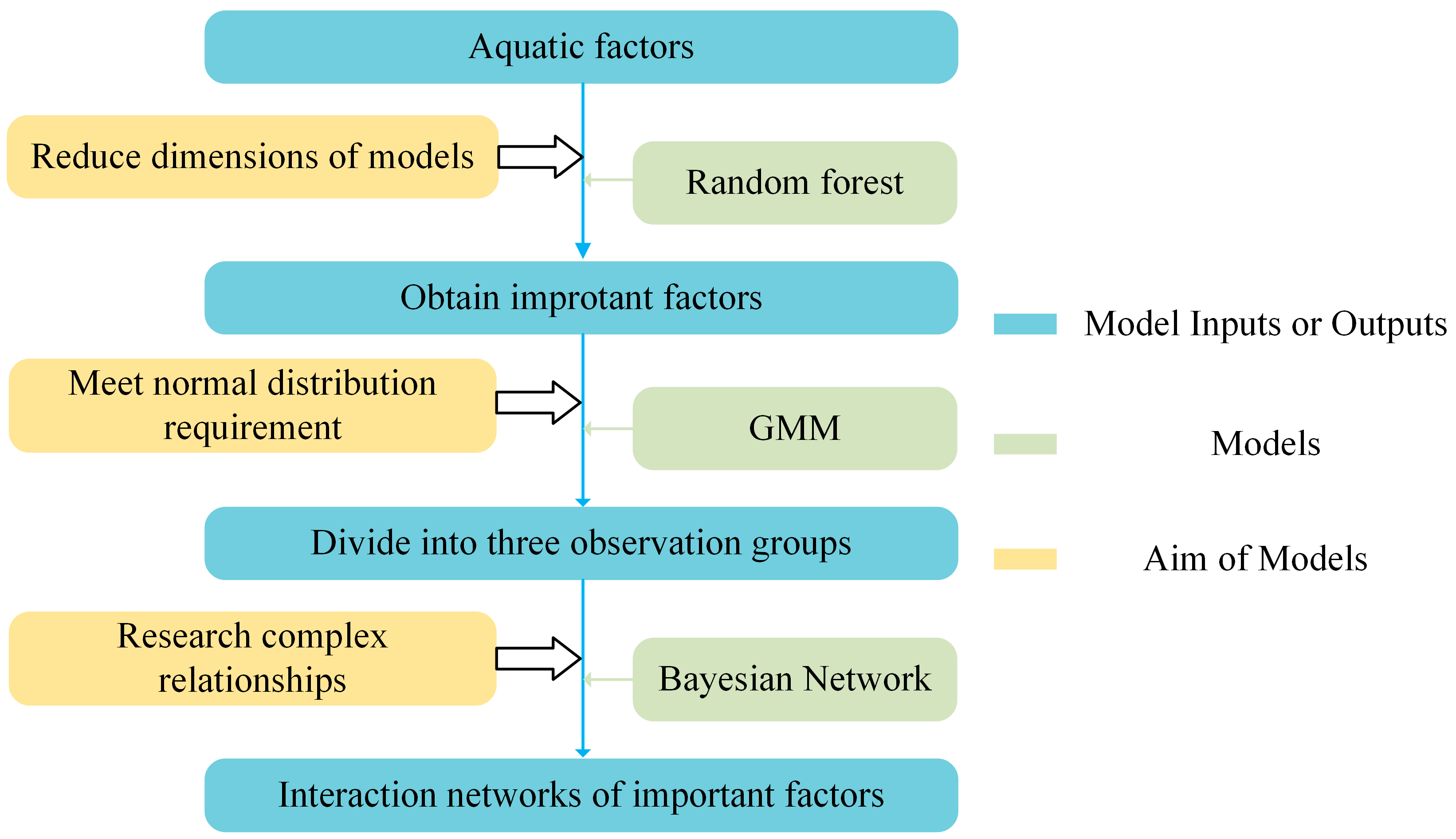
Three methods were used in the paper. (1) The RF model was employed to obtain the most important variables affecting the Fe(II) and S(−II) levels in black boom and to reduce the dimensions of the subsequent model. (2) The GMM was used to divide the observations into three groups, so that their different features could be clarified. Moreover, the observed data could be analyzed by the BN model because the data in each group had a normal distribution. (3) The BN model was used to build and analyze complex interaction relationship networks among these important factors, and threshold values were also determined by this method. Figure 2 shows the flowchart of the procedure.

3.1. Random Forest

RF is a bootstrapping aggregation method based on the classified and regression tree (CART) method [24,31]. This method resamples the data of prediction variables X to build n trees. The results of RF are a mean (for regression) or a majority vote (for classification) from the trees’ results. The features of X are also randomly sampled at every split node of the trees to ensure that the selected features are independent. This is the main difference that distinguishes RF from other bootstrapping aggregation methods. Although the identical independent distribution hypothesis is necessary for the theory development of the RF model, the violation of this property may not lead to serious consequences [32]. RF has been proven to be a very successful machine learning method for regression or classification [33,34].
In addition to classification and regression, RF is also frequently applied for important feature selection [35]. For the k th tree in RF, there would be about 1/3 of the data, called “out of bag” data O O B k , that are not used to build the model, and the variable importance measures are calculated from these data. For example, the mean square error (mse) is one of the most popular indexes used for calculating the variable importance measure. The measure of the v th feature in the k th tree based on the mse is defined as
V I M k ( v ) = i O O B k [ ( y i f k ( X ˜ i ) ) 2 ( y i f k ( X i ) ) 2 ] m
where V I M k ( v ) is the variable importance measure of the v th feature in the k th tree based on the mse, m is the number of O O B k , X i is the i th data of independent variables included in the O O B k , and y i is the corresponding dependent variable. X ˜ i is X i to which the v th feature has been permuted. The RF variable importance measure for the v th feature V I M ( v ) is defined as the mean of V I M k ( v ) .
V I M ( v ) = k = 1 n V I M ( v ) n
Other indices for the variable importance measure are defined similarly. The two most popular indices, namely, mse and node purity increase [24,34], were used in this work to identify the most important aquatic factors for S(−II) and Fe(II).

3.2. Gaussian Mixture Model

The GMM is one of most popular clustering methods based on finite mixture models [25,36]. In this method, the distribution f of observations X is specified by a probability function (PDF) by a finite mixture model of g . Suppose that, according to [37]
f ( X , Ψ ) = i = 1 G c i g i ( X , θ i )
where g i is the PDF of the i th mixture component in the finite mixture model, and θ i indicates parameters of g i . c i is the coefficient of g i , which should satisfy the condition i = 1 G c i = 1 . Ψ indicates parameters of the finite mixture model including c i and θ i .
In the GMM, each g i should be modeled by the Gaussian distribution, so that g i is characterized by two parameters: the mean μ i and the covariance matrix Σ i . g i is determined as follows
g i ( X , μ i , Σ i ) = exp [ 1 2 ( X μ i ) T Σ i 1 ( X μ i ) ] det ( 2 π Σ i )
The log likelihood for data consisting of n observations x i , i = 1 , 2 , 3 , , n according to the GMM is determined by L ( Ψ , x 1 , , x n )
L ( Ψ , x 1 , , x n ) = i = 1 n log ( f ( x i , Ψ ) )
The maximum likelihood (ML) algorithm is used for parameter estimation, and then the Bayesian Information Criterion (BIC) is applied for model selection. The open source “mclust(5.4.6)” package [36,37] in R was used in the paper to complete the GMM.

3.3. Bayesian Network

A Bayesian Network is a powerful tool that combines graph theory and probabilistic statistical theory to represent conditional dependencies among variables [26]. It is represented as a directed acyclic graph (DAG), in which the nodes of the graph are variables, and the edges indicate direct dependency relationships between these variables. This graphical model not only provides an intuitive representation of the relationships between variables but also quantifies these relationships through a joint probability distribution. According to the graph of the BN model, the distribution of the variables, excluding the root node (i.e., the node that is not connected to an edge), can be obtained as a product of conditional probability distribution [38]. Usually, a normal distribution is required for continuous variables. The global factor distribution should be obtained by multivariate Gaussian distribution, and the local distribution of every factor by univariate Gaussian distribution. It is the main reason that the GMM was applied before the BN model.
There are two steps involved when building a BN model, i.e., structure learning and parameter learning. The structure learning method is applied to build the structure of a BN with some unknown parameters. There are different kinds of structure learning algorithms, namely, constraint-based, score-based, and hybrid structure learning algorithms [26]. After comparing these algorithms, in this work, the structure of networks focused on Fe(II) and S(−II) was established by a hill-climbing algorithm, which is a type of score-based learning algorithm [39,40]. The ML estimation method was applied to estimate the unknown parameters after structure learning. Structure learning and parameter estimation were finished using the open source R package “bnlearn(4.6)” [41].
Through these steps, Bayesian Networks can effectively capture complex dependency relationships among variables, provide a mechanism for handling uncertainty, and be applied to various scenarios such as prediction and diagnosis.

4. Results and Discussions

Table 1 shows the statistical characteristics of 13 aquatic factors. The results of the Kolmogorov–Smirnov (K–S) test for empirical distribution and normal distribution are also presented.
The mean values of COD, TN, ammonia, and TP showed that the water quality in this lake bay was in a state of eutrophication. The WT of the water body showed that it was suitable for algal, mainly cyanobacteria, growth. The high concentration of CHLA showed a large accumulation of algae, but had little direct correlation with black bloom spread [23], because only dead algae decompose, which causes a sharp reduction in DO and induces the formation of black bloom [7].
Based on the national surface water quality standards of China [42], the average concentration of Fe(II) was four times larger than the upper limit for total iron, which was due to the low dissolved oxygen level and oxidation–reduction potential in the water because of the decomposition of organic matter, indicating that FeS granules formed by Fe(II) and S(−II) made the water look black. The very high value of SSC observed agreed with this. The ammonia and some compounds containing S(−II) were responsible for the odorous smell. Together, these data proved the presence of black bloom in the lake bay at this time.
The results of the K–S test demonstrated that the distributions of the 13 aquatic factors were non-Gaussian. It was necessary to divide the observations according to their different Gaussian distributions before applying the BN model.
RF was applied to select the most important factors for Fe(II) and S(−II) levels in black bloom, and the dimensions of the classification applied in the GMM were reduced. These results are shown in Figure 3.
According to the results of mse and node purity increase, the most important variables for Fe(II) with p < 0.05 were S(−II), SSC, TP, ORP, and TN. The most significant variables for S(−II) included SSC, TP, Fe(II), TN, and ammonia. Fe(II) and S(−II) were shown to be mutual key factors in black bloom, which is consistent with observational results [1]. SSC mainly depended on FeS, which was proved by a structural analysis of the black matter by scanning electron microscopy [13]; this factor was important for both Fe(II) and S(−II). Strictly speaking, Fe(II) and S(−II) were critical variables for SSC in the presence of black bloom.
Although ORP and DO exhibited almost the same level of importance for Fe(II), DO was even more important than ORP for S(−II). As shown by LASSO analysis [23], ORP showed more credible effects on Fe(II). ORP is the most sensitive index for oxidation condition measurements in bodies of water, and an euxinic environment is necessary to reduce iron and sulfate in sediments to Fe(II) and S(−II) [43]. This was another reason why ORP was selected instead of DO.
TN, TP, and ammonia played major roles in previous experimental studies [15,16,29], indicating that sediment releases more N and P during black bloom formation. TP was chosen over SP in this work due to Fe–SP adsorption [16] and the slow increase in SP. The sample was exhausted after only half a day; therefore, the effects of SP were not remarkable. The LASSO model, which also selected TP instead of SP as the explanatory variable for S(−II) and Fe(II) [23], agreed with this choice. Overall, seven factors, i.e., Fe(II), S(−II), SSC, TN, TP, ORP, and ammonia, were shown to be important for black bloom formation and were therefore selected for the GMM and BN.
After comparing 14 kinds of GMMs and classifying them in nine subsets using the BIC, a GMM model with variable volume, variable shape, ellipsoidal distribution, and equal orientation was selected for a maximum BIC value. The observations were divided into three groups with 25, 26, and 18 data points. All aquatic factor distributions in these classes were judged according to the GMM by the K–S test, and the smallest p-value was 0.0623. Figure 4 shows the map and characteristics of the three groups of observed sites. The water quality was not good in all groups, but pollution was different, so that the three groups were named “bad”, “worse”, and “worst”. This was also agreed to by the experts involved in the sampling.
The median data of the seven factors for the worst group showed that the water quality of this group was clearly worse than that of the worse and bad groups (Figure 4). For most of the variables, the observations for the bad group were better than for the worse group, as evident from the mean, median, maximum, and minimum values. On the other hand, the deviations of all variables in the worst class were larger than in the worse and bad groups, indicating that the observations in the three groups could be distinguished from each other. From the observation distributions of the different groups according to the map, the water quality in the Nanfei River was the worst, followed by that in the east of the lake bay near the river mouth, due to the river being the main pollution source of the bay [17,22], and the fact that the topography of the bay causes the matter from the river to accumulate in the east [44,45]. Generally speaking, the further away from the river mouth and land, the better the water quality, but this was also influenced by complex interactions between factors and topography.
Figure 5 shows the clustering structure and geometric characteristics obtained from the project data on to a two-dimensional subspace with density estimations [46].
As seen in Figure 5, the observations from the three groups were separated from each other, although there was some confusion between the worse and the bad classes. Although the worst class had the lowest number of data points, they were the most spread out in the subspace. This also agrees with the results showed in Figure 4. Although the number of data for the worst group was the lowest, several features of water quality indicated that in this group, black bloom was the worst.
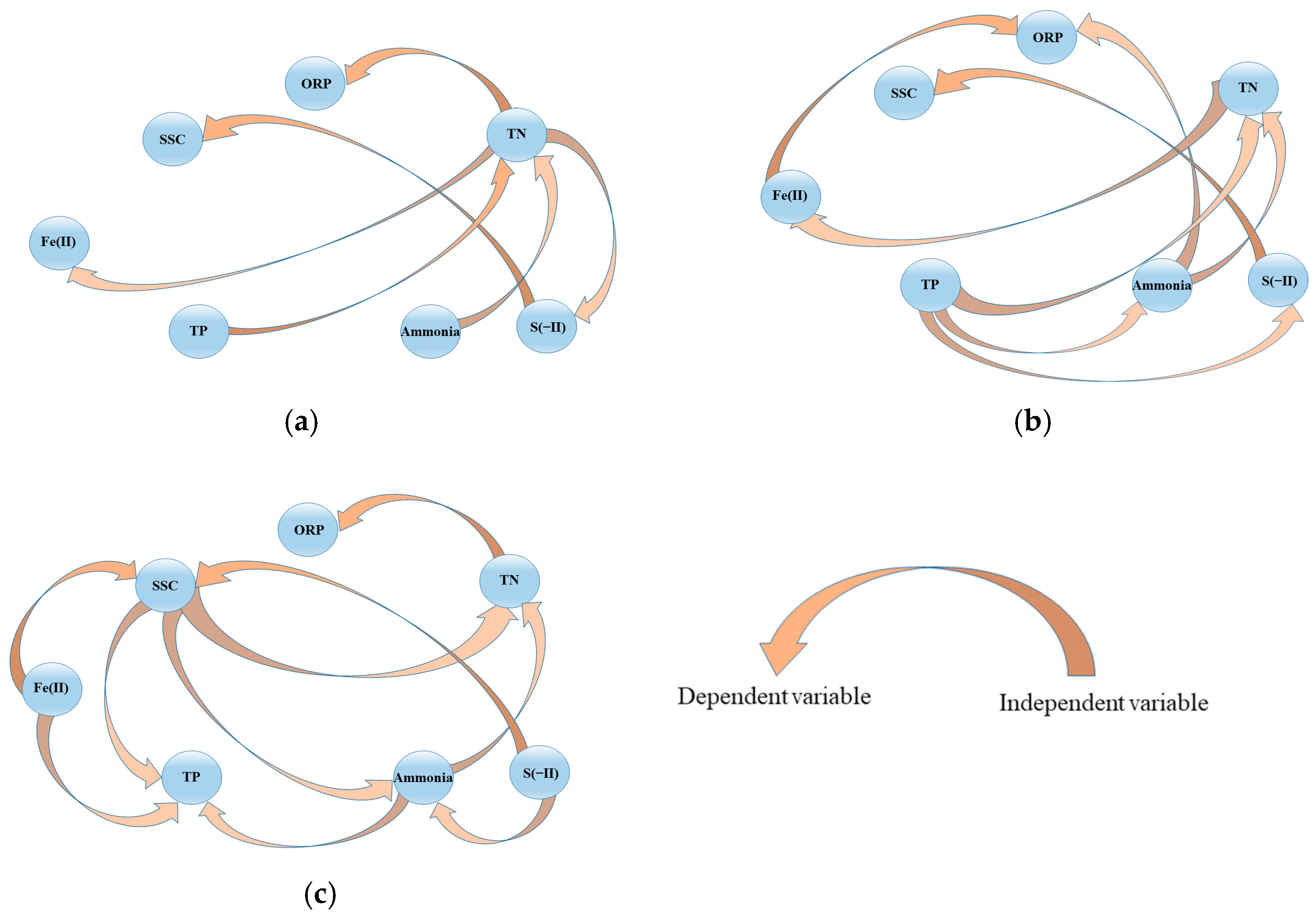
Figure 6 shows the BNs built for the three groups of observations, while Table 2 shows the coefficient of determination (R2) of every predicted factor, with the exception of the variables at the root nodes of the networks.
As Table 2 shows, the R2 of all the regression relationships in the BN models were larger than 0.6, with p-values smaller than 0.05, indicating that the results of the models could be accepted. The R2 also showed that the goodness of fit of the worst group, which was larger than 0.7, was better than that of the worse group. The statistical efficiency of the bad group’s model was the lowest, possibly because the concentrations of the aquatic factors were the highest in the worst water, so that most of the reactions were effectively controlled. The number of edges in the models also indicated that the interactions among the variables became increasingly complex with water quality deterioration.
Fe(II) and S(−II) played different roles in these networks. In the bad and worse networks, S(−II) controlled SSC production, while SSC was controlled by both Fe(II) and S(−II) in the worst group. This was because S(−II) production was greater than Fe(II) production in a more euxinic aquatic environment [47], causing FeS particles to be governed by S(−II) in the bad and worse sampled sites. Another remarkable feature was that Fe(II) and S(−II) were the root nodes in the worst group, while in the other two groups, they were not the root nodes, indicating that in the worst sample sites, which were mostly in the Nanfei River or near the river mouth, Fe(II) and S(−II) mainly derived from external sources rather than from the river estuary and were affected by other aquatic factors, such as TN and ammonia. The relationship between S(−II) and TN or ammonia is easy to understand because S(−II) promotes autotrophic denitrification [48], while denitrification can also be inhibited under high concentration of S(−II) [49].
The different characteristics of the networks also call for different governance strategies for black bloom. In heavily polluted rivers like the Nanfei River, external sources of Fe(II) and S(−II) should be strictly reduced. In polluted lake bays, TN and ammonia should be reduced, because these factors decrease the ORP and force water to become euxinic. Moreover, efforts should focus on decreasing the concentration of ammonia, as it is one of the main odorous substances. TP could also be considered for water management in the bad and worse areas because it is the root node of the networks in these two groups.
Appointing threshold values for aquatic factors could be helpful for black bloom management. Black bloom was mostly absent in the sample sites farthest from the river mouth; the average value of Fe(II) in these sites was 0.79 mg/L, which is close to the lowest concentration of Fe(II) (0.80 mg/L) that may increase DO in Chaohu Lake [22]. For ease of management, the threshold value of Fe(II) could be 0.80 mg/L. The mean value of S(−II) throughout these sites was 0.04 mg/L, which is also very close to the quantile regression result (0.043 mg/L) [22]. This could also be assigned as the threshold value of S(−II) during black bloom formation.
Based on the threshold concentrations of Fe(II) and S(−II) and the results of the BN of the worse group, the values of TP, ammonia, TN, SSC, and ORP for controlling black bloom should be 0.45 mg/L, 3.44 mg/L, 4.15 mg/L, 55 mg/L, and 135 mv, respectively. The value of Fe(II), determined by the models (inference path: S(−II)− > TP− > ammonia− > TN− > Fe(II)), was 0.91 mg/L, which agrees with the value presented above, indicating that the model is reliable.

5. Conclusions

Black bloom in lakes is a serious and complex problem in which Fe(II) and S(−II) play key roles. RF analysis showed that TN, ammonia, TP, and SSC were the aquatic factors most correlated with these two variables in water infested by black bloom. The result of RF also indicated that the ORP is a more sensitive variable than DO for Fe(II) and S(−II) production in black bloom. Considering that the concentrations of Fe(II) and S(−II) in lakes are rarely measured in China, this work shows the key indicators for better monitoring black bloom in lakes.
After clustering the observations using the GMM, the BN model showed that the interaction networks among these seven variables were different in the bad, worse, and worst water quality groups. Generally speaking, S(−II) controlled SSC production, thereby making the water look black in the bad and worse sample sites, whereas SSC determined by both S(−II) and Fe(II) in the sites with the worst water. Ammonia and TN showed the most direct importance for these two factors, while TP also influenced black bloom formation in the worse and bad groups. These results highlight the need for different management strategies to control black bloom in different water conditions. In the worst water areas, internal sources of S(−II) and Fe(II) should be strictly controlled, while in other water areas, more attention should be paid to TN and ammonia.
The threshold concentrations of the different factors to reduce black bloom were assigned based on our observations and the constructed BNs. The values of Fe(II), S(−II), TP, ammonia, TN, SSC, and ORP were 0.80 mg/L, 0.04 mg/L, 0.45 mg/L, 3.44 mg/L, 4.15 mg/L, 55 mg/L, and 135 mv, respectively. These results indicate that dredging bottom sediments and monitoring the concentrations of Fe(II) and S(−II) can help control the black and odorous water phenomenon. Additionally, as a temporary emergency measure, aeration is also an important method to quickly eliminate black bloom in the lake.

Author Contributions

Conceptualization, L.W. and Y.W.; methodology, L.W. and J.C.; software, C.X.; validation, H.N. and N.L.; formal analysis, M.X.; investigation, C.X. and Y.W.; resources, J.C.; data curation, H.N. and N.L.; writing—original draft preparation, L.W. and C.X.; writing—review and editing, M.X.; visualization, M.X.; supervision, J.C.; project administration, J.C.; funding acquisition, Y.W. and J.C. All authors have read and agreed to the published version of the manuscript.

Funding

This study was financially supported by the National Natural Science Foundation of China (Grant Nos. 51909230), the projects Research on Soil and Water Conservation and Water Ecological Environment Protection Countermeasures and Measures for the Recent Construction Project of the Flood Detention and Storage Area around Hongze Lake.

Data Availability Statement

The data presented in this study are not available on request from the corresponding author.

Conflicts of Interest

The authors declare no conflict of interest.

References

  1. Fan, C.X. Progress and Prospect in Formation of Black Bloom in Lake Taihu: A Review. J. Lake Sci. 2015, 27, 553–566. [Google Scholar]
  2. Lazaro, T.R. Urban Hydrogy; Ann Arbor Science Publishers, Inc.: Ann Arbor, MI, USA, 1979. [Google Scholar]
  3. Stahl, J.B. Black Water and Two Peculiar Types of Stratification in an Organically Loaded Strip-Mine Lake. Water Res. 1979, 13, 467–471. [Google Scholar] [CrossRef]
  4. Duval, B.; Ludlam, S.D. The Black Water Chemocline of Meromictic Lower Mystic Lake, Massachusetts, U.S.A. Intl. Rev. Hydrobiol. 2001, 86, 165–181. [Google Scholar] [CrossRef]
  5. Liu, J.J.; Lu, J.; Zhu, G.W.; Gao, M.Y.; Wen, L.; Yao, M.; Nie, Q. Occurence Characteristics of Black Patch Events and Their Influencing Factors in Lake Taihu During 2009 and 2017. J. Lake Sci. 2018, 30, 1196–1205. [Google Scholar]
  6. Guo, L. Doing Battle with the Green Monster of Taihu Lake. Science 2007, 317, 1166. [Google Scholar] [CrossRef]
  7. Shen, A.C.; Xu, Z.A.; Wu, D.H. Relationships between Accumulation and Dying of Cyanobacteria and Black Spot. J. Hydroecol. 2012, 33, 68–72. [Google Scholar]
  8. Lu, G.H.; Ma, Q.; Zhang, J.H. Analysis of Black Water Aggregation in Taihu Lake. Water Sci. Eng. 2011, 4, 374–385. [Google Scholar]
  9. Shi, K.; Zhang, Y.L.; Zhou, Y.Q.; Liu, X.H.; Zhu, G.W.; Qin, B.Q.; Gao, G. Long-Term Modis Observations of Cyanobacterial Dynamics in Lake Taihu: Responses to Nutrient Enrichment and Meteorological Factors. Sci. Rep. 2017, 7, 40326. [Google Scholar] [CrossRef] [PubMed]
  10. Han, C.; Ding, S.; Yao, L.; Shen, Q.; Zhu, C.; Wang, Y.; Xua, D. Dynamics of Phosphorus-Iron-Sulfur at the Sediment-Water Interfaceinfluenced by Algae Blooms Decomposition. J. Hazard. Mater. 2015, 300, 329–337. [Google Scholar] [CrossRef]
  11. Lu, X.; Liu, C.; Yin, H.B.; Fan, C.X. The Main Sulfur-Containing Odorous Compounds and Their Forming Mechanisms in Waters During Bio-Induced Black Bloom. J. Lake Sci. 2015, 27, 583–590. [Google Scholar]
  12. Lu, X.; Fan, C.X.; He, W.; Deng, J.C.; Yin, H.B. Sulfur-Containing Amino Acid Methionine as the Precursor of Volatile Organic Sulfur Compounds in Algea-Induced Black Bloom. J. Environ. Sci. 2013, 25, 33–43. [Google Scholar] [CrossRef] [PubMed]
  13. Fan, C.X.; Shen, Q.S. Identification of Black Suspended Particles in the Algae-Induced Black Bloom Water Column. J. Lake Sci. 2015, 27, 591–598. [Google Scholar]
  14. Wang, C.L.; Zhang, Y.; Zhang, N.H.; Qian, X.; Kong, F.X. Analysis of Meteorological Factors of Forming Feculent and Anaerobic Water Aggreation Induced by Algal Bloom in Taihu Lake. Environ. Sci. 2011, 32, 401–408. [Google Scholar]
  15. Liu, G.F.; He, J.; Fan, C.X.; Zhang, L.; Shen, Q.S.; Zhong, J.C.; Yan, S.H. Environment Effects of Algae-Caused Black Spots: Impacts on Fe-Mn-S Cycles in Water-Sediment Interface. Environ. Sci. 2010, 31, 2652–2660. [Google Scholar]
  16. Liu, G.F.; Fan, C.X.; Zhang, L.; Shen, Q.S.; Wang, Z.D.; Han, S.Q. Environment Effects of Algae-Caused Black Spots Iii: Impacts on Fe-S-P Cycle in Water-Sediment Interface. China Environ. Sci. 2014, 34, 3199–3206. [Google Scholar]
  17. Shen, Q.S.; Fan, C.X.; Liu, C.; Chen, C. The Limiting Factor to the Outbreak of Lake Black Bloom:Roles of Ferrous Iron and Sulfide Ions. Clean Soil Air Water 2018, 46, 1800305. [Google Scholar] [CrossRef]
  18. Canfield, D.E., Jr.; Linda, S.B.; Hodgson, L.M. Relations between Color and Some Limnological Characteristics of Florida Lakes. JAWRA 1984, 20, 323–329. [Google Scholar]
  19. Sugiura, N.; Utsumi, M.; Wei, B.; Iwami, N.; Okano, K.; Kawauchi, Y.; Maekawa, T. Assessment for the Complicated Occurrence of Nuisance Odours from Phytoplankton and Environmental Factors in a Eutrophic Lake. Lakes Reserv. Res. Manag. 2004, 9, 195–201. [Google Scholar] [CrossRef]
  20. Dzialowski, A.R.; Smith, V.H.; Huggins, D.G.; de Noyelles, F.; Lim, N.-D.; Baker, D.S.; Beurya, J.H. Development of Predictive Models for Geosmin-Related Taste and Odor in Kansas, USA, Drinking Water Reservoirs. Water Res. 2009, 43, 2829–2840. [Google Scholar] [CrossRef]
  21. Wang, Y.L.; Wang, L.; Hua, Z.L.; Ding, S.M. The Relationships of Velocity, Dissolved Oxygen with Fe2+, S2− in Black Bloom Region on Nanfei River Estuary of Lake Chaohu. J. Lake Sci. 2016, 28, 710–717. [Google Scholar]
  22. Wang, Y.L.; Wang, L.; Hua, Z.L. The Relationships of Different Concentration Fe2+, S2− with Hydrodynamics, Do in Black Bloom Water Based on Quantile Regression Method. China Environ. Sci. 2018, 38, 627–633. [Google Scholar]
  23. Wang, L.; Wang, Y.L.; Cheng, H.M.; Cheng, J.L. Identifying the Driving Factors of Black Bloom in Lake Bay through Bayesian Lasso. Int. J. Environ. Res. Public Health 2019, 16, 2492. [Google Scholar] [CrossRef] [PubMed]
  24. Brieman, L. Random Forests. Mach. Learn. 2001, 45, 5–32. [Google Scholar] [CrossRef]
  25. Fraley, C.; Rafery, A.E. Model-Based Clustering, Discriminant Analysis, and Density Estimation. J. Am. Stat. Assoc. 2002, 97, 611–631. [Google Scholar] [CrossRef]
  26. Pearl, J. Causality: Models, Reasoning and Inference, 2nd ed.; Cambridge University Press: Cambridge, UK, 2009. [Google Scholar]
  27. Wei, F. Mornitoring and Analytic Method for Water and Waste Water; China Environmental Publisher: Beijing, China, 2002; pp. 88–129. [Google Scholar]
  28. Cline, J.D. Spectrophotometric Determination of Hydrogen Sulfide in Natural Waters. Limnol. Oceanogr. 1969, 14, 454. [Google Scholar] [CrossRef]
  29. Liu, G.F.; Shen, Q.S.; Zhang, L.; Fan, C.X.; Zhong, J.C.; Yan, S.H. Environment Effects of Algae-Caused Black Spots: Driving Effects on the N,P Changes in the Water-Sediment Interface. Environ. Sci. 2010, 31, 2917–2924. [Google Scholar]
  30. Lu, G.H.; Ma, Q. Monitoring and Analysis on “Black Water Aggregation” in Lake Taihu, 2009. J. Lake Sci. 2010, 22, 481–487. [Google Scholar]
  31. Speybroeck, N. Classification and Regression Trees. Int. J. Public Health 2012, 57, 243–246. [Google Scholar] [CrossRef] [PubMed]
  32. Hastie, T.; Tibshirani, R.; Friedman, J. The Elements of Statistical Learning: Data Mining, Inference, and Prediction, 2nd ed.; Springer: New York, NY, USA, 2009. [Google Scholar]
  33. Antia, S.T.; Edwin, R.; Bodan, Z. Comparison of Support Vector Machine and Random Forest Algorithms for Invasive and Expansive Species Classification Using Airborne Hyperspectral Data. Remote Sens. 2020, 12, 516. [Google Scholar] [CrossRef]
  34. Svetnik, V.; Liaw, A.; Tong, C.; Culberson, J.C.; Sheridan, R.P.; Feuston, B.P. Random Forest: A Classification and Regression Tool for Compound Classification and Qsar Modeling. J. Chem. Inf. Comput. Sci. 2003, 43, 1947. [Google Scholar] [CrossRef]
  35. Wang, Y.L.; Wang, L.; Cheng, J.L.; He, C.D.; Cheng, H.M. Recognizing Crucial Aquatic Factors Influencing Greenhouse Gas Emissions in the Eutrophication Zone of Taihu Lake, China. Sustainability 2019, 11, 5160. [Google Scholar] [CrossRef]
  36. Scrucca, L.; Fop, M.; Murphy, T.B. Mclust 5 Clustering, Classification and Density Estimation Using Gaussian Finite Mixture Models. R J. 2016, 8, 289–317. [Google Scholar] [CrossRef] [PubMed]
  37. Fraley, C.; Rafery, A.E. Model-Based Methods of Classification: Using the Mclust Software in Chemomertics. J. Stat. Softw. 2007, 18, 1–13. [Google Scholar] [CrossRef]
  38. Pearl, J. Probabilistic Reasoning in Intelligent Systems: Networks of Plausible Inference; Morgan Kaufmann Publishers Inc.: San Francisco, CA, USA, 1988. [Google Scholar]
  39. Russell, S.; Norvig, P. Artificial Intelligence: A Modern Approach, 3rd ed.; Prentice Hall: Upper Saddle River, NJ, USA, 2009. [Google Scholar]
  40. Neapolitan, R.E. Learning Bayesian Networks; Prentice Hall: Englewood Cliffs, NJ, USA, 2003. [Google Scholar]
  41. Scutari, M. Learning Bayesian Networks with the Bnlearn R Package. J. Stat. Softw. 2010, 35, 1–21. [Google Scholar] [CrossRef]
  42. GB 3838-2002; National Surface Water Quality Standard. State Environmental Protection Administration (China): Beijing, China, 2002.
  43. Fan, C.X.; Zhou, Y.Y.; Wu, Q.L. The Effects and Processes of Lake Sediment Interface; Science Press: Beijing, China, 2013. [Google Scholar]
  44. Hua, Z.L.; Liu, X.D.; Chu, K.J.; Gu, L.; Wang, L. Numerical Simulation of Water Flow and Pollutant Transport Based on Boundary Fitting; Science Press: Beijing, China, 2013. [Google Scholar]
  45. Wang, Y.L. Research on Parameters Sensitivity and Optimization Determination of Chaohu Lake Efdc Eutrophication Model; Hohai University: Nanjing, China, 2018. [Google Scholar]
  46. Scrucca, L. Dimension Reduction for Model-Based Clustering. Stat. Comput. 2010, 20, 471–484. [Google Scholar] [CrossRef]
  47. Zhang, W.; Li, Q.M.; Wang, X.X.; Din, Y.; Sun, J.X. Reducing Organic Substances from Anaerobic Decomposition of Hydrophytes. Biogeochemistry 2009, 94, 1–11. [Google Scholar] [CrossRef]
  48. Vile, M.A.; Bridgham, S.D.; Wieder, R.K. Response of Anaerobic Carbon Mineralization Rates to Sulfate Amendments in a Boreal Peatland. Ecol. Appl. 2003, 13, 720–734. [Google Scholar] [CrossRef]
  49. Bartacek, J.; Manconi, I.; Sansone, G.; Murgia, R.; Lens, P. Divalent Metal Addition Restores Sulfide-Inhibited N2o Reduction in Pseudomonas Aeruginosa. Nitric Oxide 2010, 23, 101–105. [Google Scholar] [CrossRef]
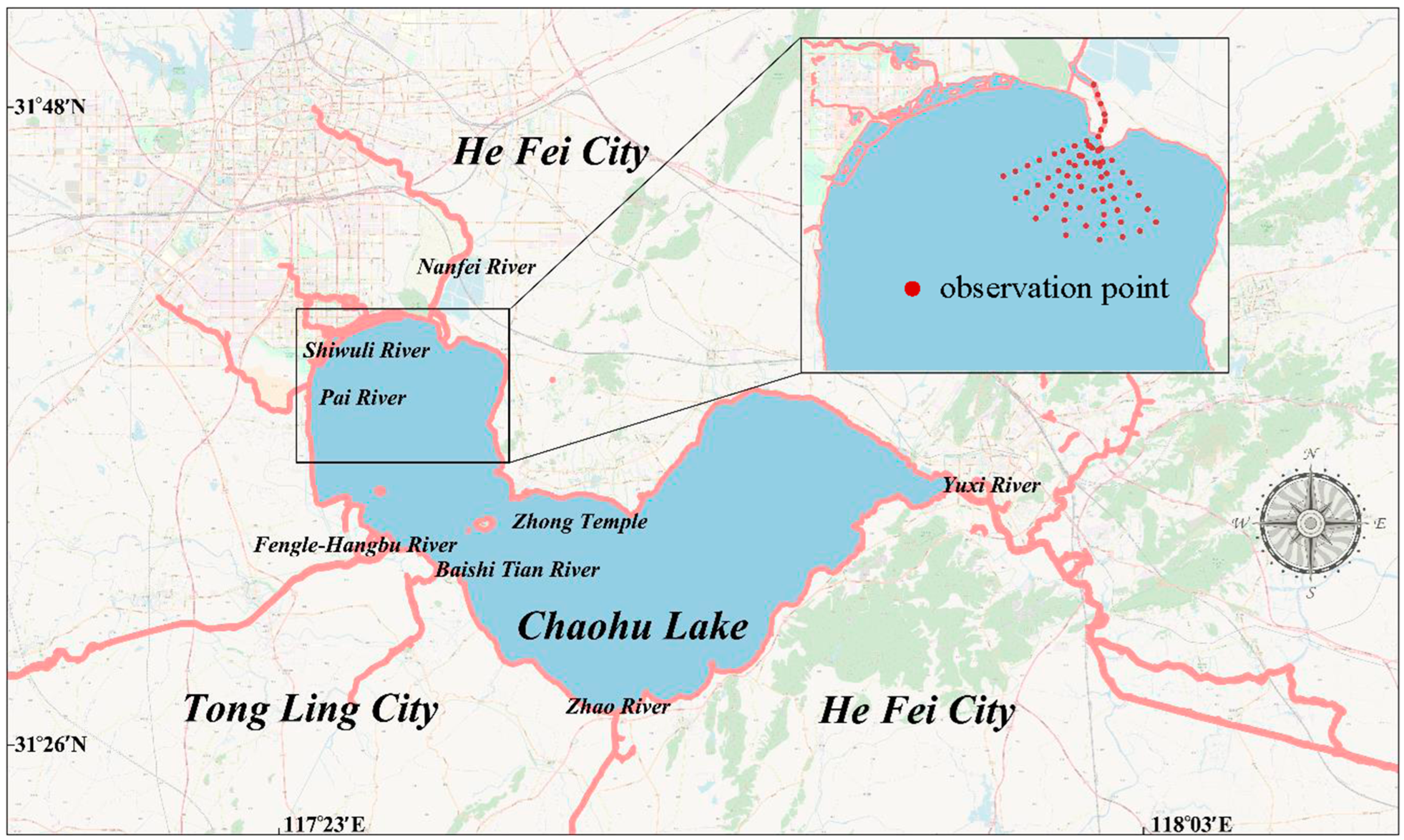
Figure 1. The region of Chaohu Lake and the sampling sites.
Water 16 03120 g001
Figure 2. The flowchart of the procedure.
Water 16 03120 g002
Figure 3. The important factors for (a) Fe(II); (b) S(−II).
Water 16 03120 g003
Figure 4. Characteristics of the three groups of observations.
Water 16 03120 g004
Figure 5. The project data from the Gaussian Mixture Model (GMM).
Water 16 03120 g005
Figure 6. Bayesian Network (BN) model for the three groups. (a) Bad; (b) worse; (c) worst.
Water 16 03120 g006
Table 1. Statistical observations (n = 69).
Item ***MinimumMeanSD *MaximumK–S Test (D/p) **Normal
SP (mg/L)0.02 0.20 0.31 1.43 0.332/<0.01No
TP (mg/L)0.09 0.52 0.55 2.94 0.271/<0.01No
TN (mg/L)0.66 3.72 3.46 14.99 0.209/<0.01No
Ammonia (mg/L)0.33 3.00 2.94 12.44 0.287/<0.01No
S(−II) (mg/L)0.02 0.05 0.02 0.15 0.203/<0.01No
Fe(II)(mg/L)0.24 1.27 0.94 5.51 0.279/<0.01No
pH6.837.940.398.350.193/0.011No
DO (mg/L)1.85 6.50 1.58 8.43 0.202/<0.01No
WT (°C)23.80 25.42 1.79 31.80 0.258/<0.01No
ORP (mV)−86117531680.209/<0.01No
COD (mg/L)61.33 78.74 8.00 110.86 0.194/0.011No
CHLA (mg/m3)17.0647.9824.64165.460.210/<0.01No
SSC (mg/L)410618611880.331/<0.01No
Note(s): * SD: standard deviation. ** Results of K–S test are non-unit; p > 0.05 indicates normal variable distribution. *** SP: soluble phosphorus, TP: total phosphorus, TN: total nitrogen, DO: dissolved oxygen, WT: water temperature, ORP: oxidation–reduction potential, COD: O2 demand, CHLA: chlorophyll a, SSC: suspended sediment concentration.
Table 2. Coefficient of determination (R2) of the Bayesian Networks (BNs).
Fe(II)S(−II)TNTPAmmoniaSSCORP
Worst//0.98 0.96 0.73 0.76 0.89
Worse0.62 0.63 0.75 /0.93 0.66 0.79
Bad0.61 0.63 0.65 /0.91 0.60 0.63
Disclaimer/Publisher’s Note: The statements, opinions and data contained in all publications are solely those of the individual author(s) and contributor(s) and not of MDPI and/or the editor(s). MDPI and/or the editor(s) disclaim responsibility for any injury to people or property resulting from any ideas, methods, instructions or products referred to in the content.