An Interpretable CatBoost Model Guided by Spectral Morphological Features for the Inversion of Coastal Water Quality Parameters

Abstract

Chlorophyll-a (Chla) and total suspended solid (TSS) concentrations are important parameters for water quality assessment, and in recent years, machine learning has been shown to have great potential in this field. However, current water quality parameter inversion models lack interpretability and rarely consider the morphological characteristics of the spectrum. To address this limitation, we used Sentinel-3 OLCI data to construct an interpretable CatBoost model guided by spectral morphological characteristics for remote sensing monitoring of Chla and TSS along the coast of Fujian. The results show that the coastal waters of Fujian Province can be divided into five clusters, and the areas of different clusters will change with the alternation of seasons. Clusters 2 and 4 are the main types of coastal waters. The CatBoost model combined with spectral feature engineering has a high accuracy in predicting Chla and TSS, among which Chla is slightly better than TSS (R² = 0.88, MSE = 8.21, MAPE = 1.10 for Chla predictions; R² = 0.77, MSE = 380.49, MAPE = 2.48 for TSS predictions). We further conducted an interpretability analysis on the model output and found that the combination of BRI and TBI indexes composed of bands such as b8, b9, and b10 and the fluctuation of spectral curves will have a significant impact on the prediction of model output. The interpretable CatBoost model based on spectral morphological features proposed in this study can provide an effective technical means of estimating the chlorophyll-a and total suspended particulate matter concentrations in the coastal areas of Fujian.

1. Introduction

As an important part of the natural water cycle [1], coastal waters have a profound impact on human production and life. Currently, with the development of science and technology and the impact of human activities, the pollution of coastal waters has become increasingly serious [2,3,4]. Factory sewage and aquaculture wastewater flow into offshore waters through surface runoff, posing a serious threat to coastal water quality ecology [5,6,7]. To protect the coastal ecological environment, it is necessary to conduct the rapid and accurate monitoring of the water environment. Chlorophyll-a (Chla) concentration is one of the most important indicators for studying global marine phytoplankton dynamics and the carbon cycle, and for eutrophication assessment [8]. The total suspended solid (TSS) concentration affects water transparency and light propagation in water and can even affect water temperature through absorption [9]. In the past few years, Chla and TSS have therefore often been used as important indicators for evaluating water environments [10,11,12].

It is not feasible to assess water quality parameters over a large area using only data from field surveys. Satellite remote sensing technology is characterized by long time series, large range, and high timeliness and has become an important means of water environment monitoring [13], among which ocean color remote sensing is the most effective method for monitoring global oceans and aquatic ecosystems [14]. In the past, scholars have developed various algorithms for estimating chlorophyll-a (Chla) and total suspended solid (TSS) concentrations, such as the normalized difference chlorophyll index (NDCI) [15], an analysis algorithm proposed based on the results of bio-optical modeling. In addition, there are empirical relationship inversion methods based on the ratio method [16,17], three-band algorithm [18,19,20], and four-band algorithm [21,22]. However, remote sensing reflectivity and water quality parameters often present a complex nonlinear relationship [23], which is difficult to express using an empirical formula or statistical model. Machine learning methods that can handle complex nonlinear characteristics have thus been widely used for the inversion of water quality parameters in recent years [24], for example, the Chla inversion model designed using convolutional neural networks (CNNs) and spatiotemporal fusion algorithms (STFs) [25]. There are also studies that use seven machine learning algorithms such as XGBoost, random forest, and GBDT to establish various band combinations to estimate the TSS concentration of global lakes. The results show that GBDT has great potential for estimating TSS [26].

In fact, the estimation of water quality parameters will be affected by many factors, such as the optical variability of water bodies. The optical variability of water comes from active optical substances in water [27], such as chlorophyll-a and total suspended solid concentrations, and colored dissolved organic matter (CDOM). These optical components interact with each other, resulting in uncertainty in inversion. Even if the spectral features constructed based on experience and analysis can reduce the impact of non-target parameters on target parameters, they often lack generalization and large-scale application capabilities. The spectral morphological characteristics of water bodies just reflect the interaction of optical components of water bodies. Although machine learning models have achieved satisfactory results in the inversion of water quality parameters, due to their black box problem [28], it is difficult for us to explain why the model makes such predictions.

Therefore, based on the above research we introduced an interpretable method based on game theory, combined with spectral morphological characteristics, OLCI ocean color data, and the CatBoost model, established the estimation model of Chla and TSS in the coastal area of Fujian Province, and drew spatial distribution maps to analyze their spatiotemporal variation characteristics in the coastal area of Fujian Province, China. The main objectives of this study were to (1) accurately estimate the concentrations of Chla and TSS in the coastal area of Fujian Province; (2) provide a reasonable explanation for the estimation results and analyze the influence of different characteristics of spectral curves on the estimation results; and (3) draw the spatial distribution and spatiotemporal distribution maps of Chla and TSS in the coastal area of Fujian Province, China. The innovation of this study is that by using the traditional band combination as the modeling feature, the morphological characteristics of the water spectral curve are considered. The accuracy of Chla and TSS prediction is enhanced via the joint modeling of the two types of features. Concurrently, the SHAP interpretability framework is employed to analyze the interpretability of the model’s prediction results to enhance the credibility of the model.

2. Study Area and Data Preprocessing

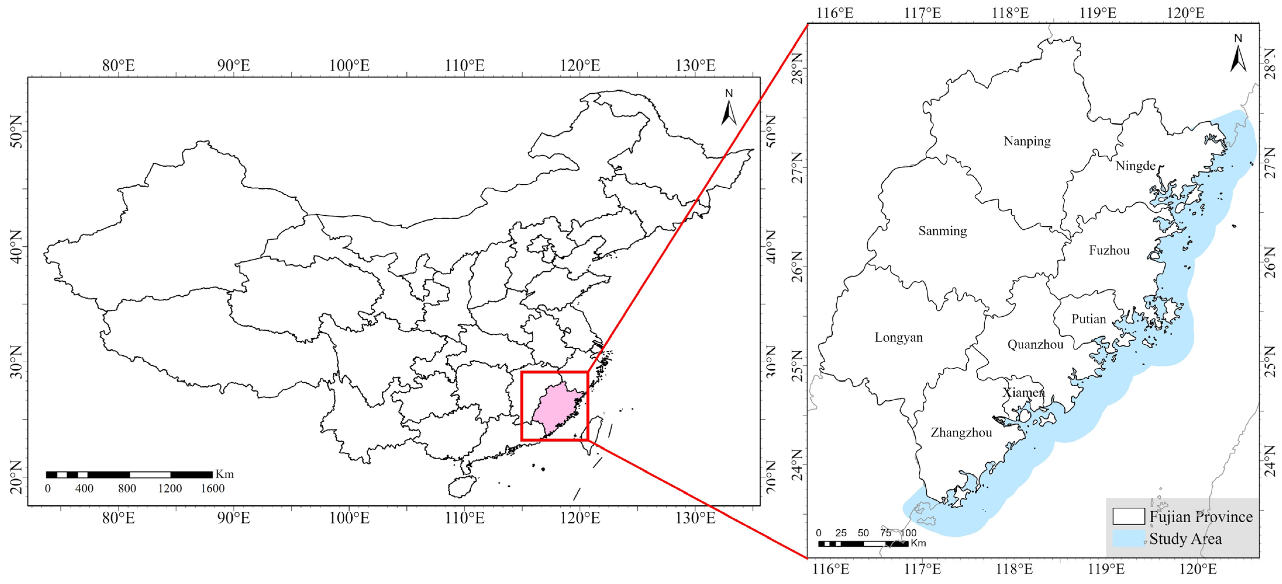
2.1. Study Area

As a coastal province of China, Fujian has the second longest coastline in China, enabling it to develop a rich marine aquaculture industry and maritime transportation industry. However, with the process of urbanization, human activities along the coast are gradually changing the coastal water environment, and the discharge of industrial wastewater is gradually gathering in coastal waters and impacting the water system. Simultaneously, the aquaculture wastewater produced by the aquaculture industry is also causing eutrophication of nearshore water bodies, eventually forming red tides, which has a serious impact on the production and life of coastal cities. It is therefore necessary to perform rapid and accurate monitoring of the coastal water environment in Fujian Province.

Fujian Province is located in the southeast of China, between 23°31′–28°18′ N and 115°50′–120°43′ E. Due to Fujian Province’s unique subtropical monsoon climate [29], in subsequent seasonal studies, we define March, April, and May as spring, June to September as summer, October and November as autumn, and December, January, and February as winter. The study area for this study is shown in Figure 1. This map was produced using vector data downloaded from the China National Geographic Information Service Platform (https://www.tianditu.gov.cn/) (accessed on 20 November 2024).

2.2. Sentinel-3 OLCI Data Processing

This study used the Sentinel-3 OLCI data product from the European Space Agency. The satellite was launched in February 2016 with a spatial resolution of 300 m and a total of 21 spectral bands [30]. The introduction and function of each band can be found on the ESA official website (https://sentiwiki.copernicus.eu/web/olci-products) (accessed on 20 November 2024).

Since the signals received by satellite sensors are affected by the atmosphere, atmospheric correction processing is required before using satellite data. In this study, we used the C2RCC algorithm to perform atmospheric correction on the Sentinel-3 OLCI. Case 2 Regional Coast Color (C2RCC) is an atmospheric correction algorithm based on an artificial neural network [21,31,32], using data measured by satellite sensors at the top of the atmosphere to invert the photochemical properties of water [33]. Studies have shown that data corrected via C2RCC can well preserve the spectral characteristics of water bodies [34]. We first performed C2RCC processing on the downloaded Sentienl-3 OLCI Level 1 product in the SNAP software (version 10.0) package to output the water remote sensing reflectance (Rrs). Because some bands of Sentinel-3 OLCI data are auxiliary bands involved in atmospheric correction, the output Rrs will only have 16 bands. We combined 15 bands in the wavelength range from 400 nm to 900 nm into one image, cropped the study area, and finally formed the image dataset.

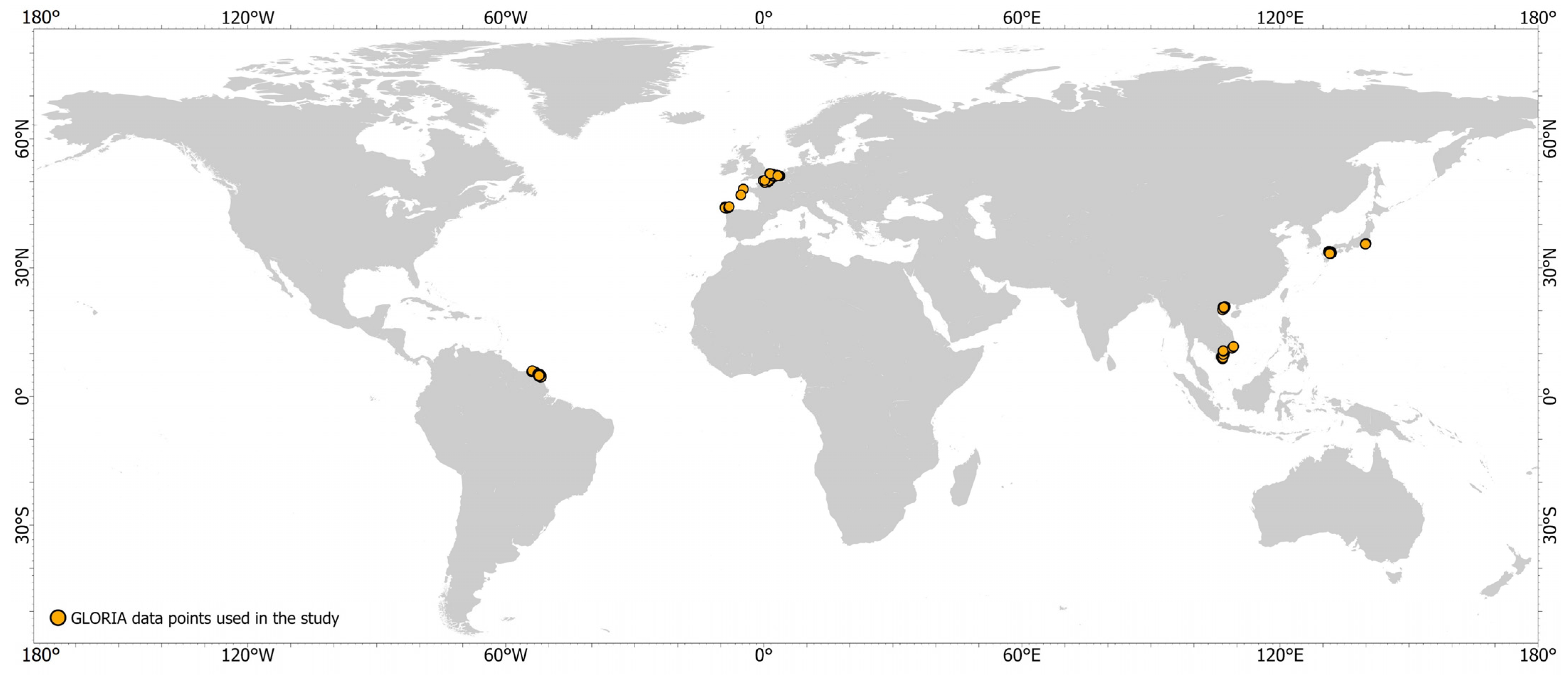
2.3. GLORIA Dataset Simulates in Situ Data

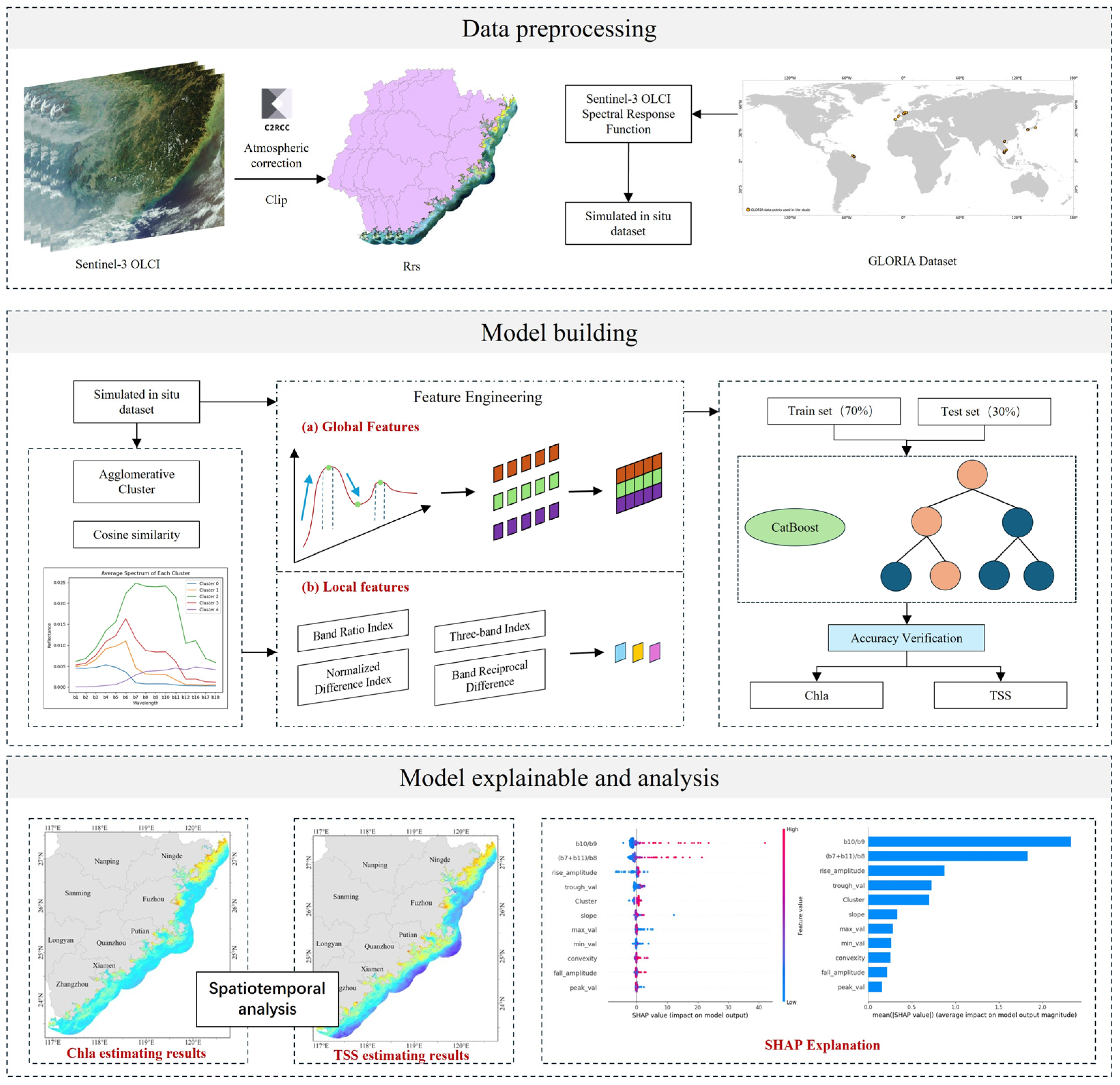
The GLORIA dataset [35] is a collaborative effort, contributed to by 59 research institutions around the world. It comprises a total of 7572 water body hyperspectral-remote sensing-reflectance measurement datasets from 450 different water bodies, with a spectral measurement interval of 1 nm and a wavelength range from 350 nm to 900 nm. The measured points selected for modeling in this study are shown in Figure 2. The study points are mainly distributed in Southeast Asia, western Europe, and northern South America. Each spectral curve includes the data for at least one in situ water quality measurement of chlorophyll-a, total suspended solids, absorption by dissolved substances, and Secchi depth. We screened a total of 7572 spectral curves, deleted the curves with incomplete spectral information between 400 nm and 900 nm, and selected coastal water types and data with chlorophyll-a and total suspended solid concentrations. Finally, we obtained 340 pairs of simulated in situ datasets for model construction.

We then used Equation (1) [36] to resample the 340 spectral curves to obtain a spectral curve dataset with the same spectral interval as OLCI.

$$R={\displaystyle \frac{{\displaystyle {\int }_{400}^{900}SRF(\lambda )}Rrs(\lambda )d\lambda }{{\displaystyle {\int }_{400}^{900}SRF(\lambda )}d\lambda }}$$

(1)

where $SRF\left(\lambda \right)$ is the spectral response function of Sentinel-3 OLCI, and $R_{rs}\left(\lambda \right)$ is the measured water remote sensing reflectance, which here refers to the water remote sensing reflectance in the GLORIA dataset.

3. Methods

As shown in Figure 3, the overall technical route of this study includes three parts: data preprocessing, model building, and interpretability and analysis. Data preprocessing is described in detail in Section 2.2 and Section 2.3. Model building mainly includes water body spectral classification, feature engineering construction, and model training.

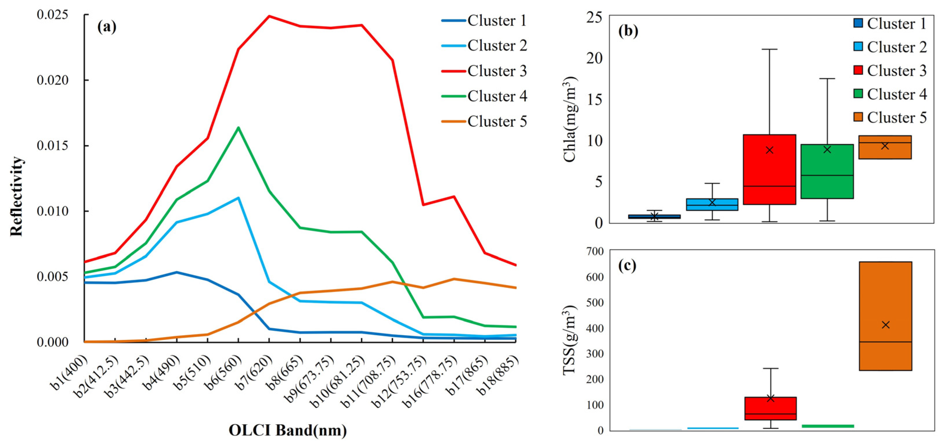
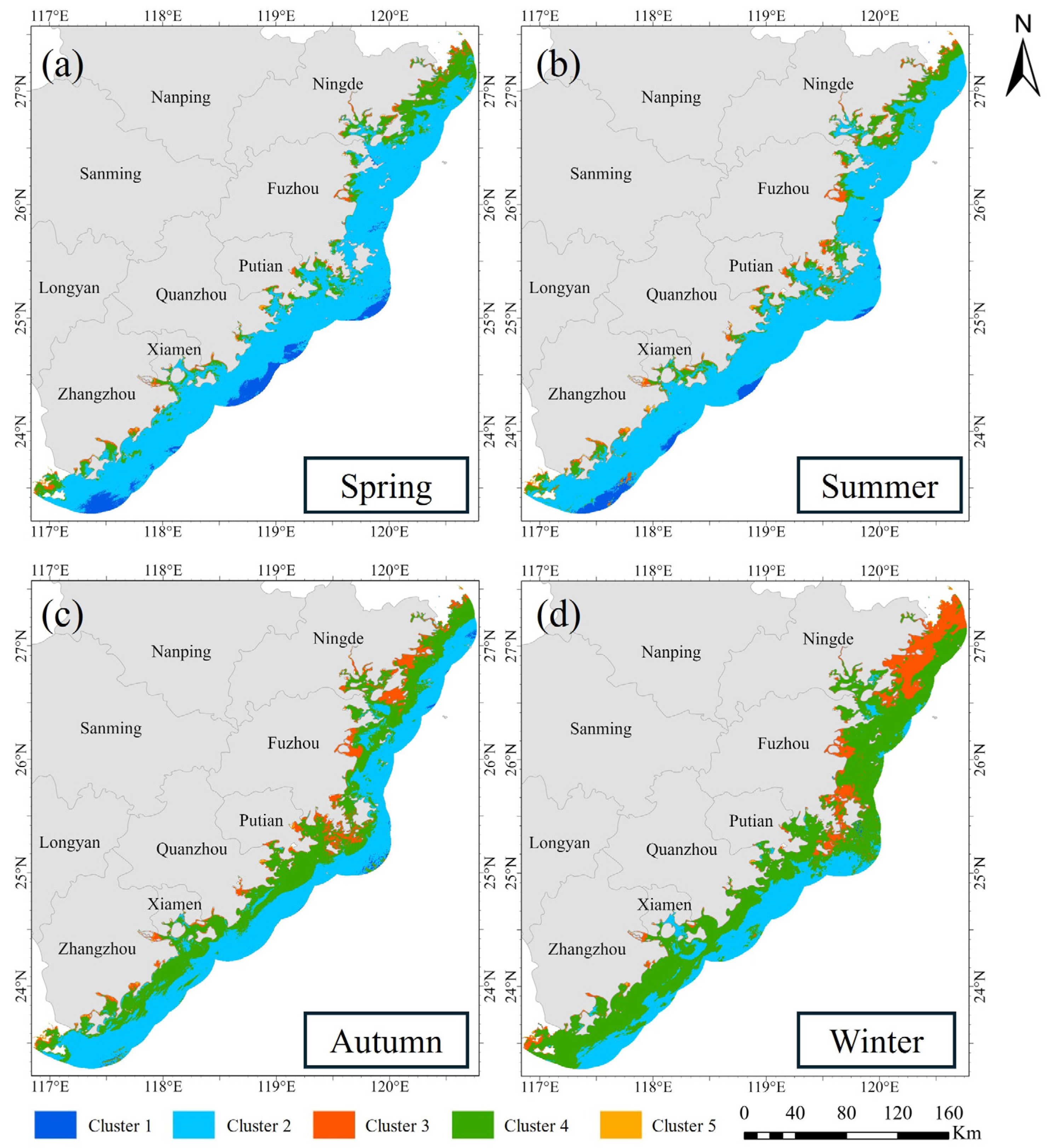
3.1. Water Spectral Classification

The spectral curve of water is the result of the combined influence of multiple water quality parameters, which have different contents and will thus cause the water body to present different spectral curve characteristics [37,38]. To explore the influence of different water quality parameter concentrations on the spectral direction and shape, this study therefore used the agglomerative clustering method combined with cosine similarity to cluster 340 spectral curves.

Many studies [39,40,41] have applied cluster analysis to the classification of objects in remote sensing images, and agglomerative clustering is a bottom-up clustering process [42]. In this study, we used agglomerative clustering to treat each data point as a separate cluster, and then we measured the distance between clusters using cosine similarity (Equation (2)) [43] and merged the two most similar clusters, finally obtaining the clustering results of the five water spectral curves.

$$similarity={\displaystyle \frac{{\displaystyle \sum _{i=1}^n{A}_i\times B_i}}{\sqrt{{\displaystyle \sum _{i=1}^n{\left(A_i\right)}^2}}\times \sqrt{{\displaystyle \sum _{i=1}^n{\left(B_i\right)}^2}}}}$$

(2)

where $A_i$ and $B_i$ represent the components of curves A and B, respectively.

The final clustering results of 340 spectral curves are shown in Figure 4. Figure 4b,c show the concentrations of water quality parameters in different water body types. From cluster 1 to cluster 5, the average values of Chla are 0.7 mg/m³, 2.4 mg/m³, 8.7 mg/m³, 8.8 mg/m³, and 9.2 mg/m³, respectively, and the average values of TSS are 2.5 g/m³, 16.5 g/m³, 124.0 g/m³, 18.9 g/m³, and 411.1 g/m³, respectively. Figure 4a shows how different Chla and TSS concentrations affect the shape of the spectral curve of the water body. From the perspective of the slope and convexity of the spectral curve, clusters 1 and 5 exhibit the smallest changes; from the statistical information, we can see that cluster 1 has the lowest Chla and TSS concentrations. The spectral curve shows a small slope in the blue light band, a very small increase in reflectivity, and a subsequent gradual decrease. This type of water body is generally distributed in offshore areas far from land. Cluster 5 has an extremely high TSS concentration, showing a completely opposite trend to cluster 1. Its spectral curve gradually increases slightly with an increasing wavelength. This trend is similar to the spectral curve of land and is generally distributed in silt or sand close to land. Clusters 2 and 4 show two types of spectral curves commonly seen in coastal waters, which present the first reflection peak at the green band (560 nm), after which the reflectivity gradually decreases. As the Chla concentration increases, the second reflection peak is likely to appear at the 10 band (681.25 nm). Cluster 3 shows the spectral curve of water bodies with high TSS concentrations near the coast, which presents a trough with a slope close to 0 from the green band (560 nm) to the red band (681.25 nm), and a small reflection peak in the near-infrared band (778.75 nm). The above analysis shows that different concentrations of water quality parameters will have different effects on the spectral curve of water bodies. However, when the water body contains an extremely high TSS concentration, its curve characteristics may be masked, resulting in the inability to identify the concentration distribution of Chla. In this case, the estimation of the Chla concentration needs to be assisted by the local characteristics of the curve. By constructing feature engineering of the curve, we can better estimate the status of water quality parameters.

Based on the spectral curve classification results, this study inputs all remote sensing images, calculates the cosine similarity between each pixel spectral curve and the five spectral curves in the clustering results, and classifies the pixel into the spectral curve with the highest cosine similarity, generating a dataset of water body classification results for the coastal waters of Fujian Province from recent years for subsequent model construction. Figure 5 shows the seasonal classification results of coastal water bodies in Fujian Province.

In Figure 5, the coastal waters of Fujian Province mainly comprise cluster 2 and cluster 4 water bodies. From the perspective of temporal changes, the area of cluster 4 water bodies in coastal waters increases in the autumn and winter seasons, indicating that the Chla concentration along the coast of Fujian Province increases during this period; in July and August, the area of cluster 4 water bodies decreases, the area of cluster 2 water bodies increases, and cluster 1 water bodies appear in the marginal areas close to the open sea. From the perspective of regional water body type distribution, the eastern coast of Ningde City is in cluster 4 water bodies all year round and they will gradually “diffuse” to the open sea area in autumn and winter. In most bays, the water body types in July and August are basically cluster 2 water bodies. The area of cluster 2 water bodies decreases in autumn and winter, and the area of cluster 4 water bodies increases. Cluster 3 water bodies have a relatively obvious temporal and spatial distribution pattern, and a large area appears in the eastern area of Sansha Bay, Ningde City, in March and December, followed by some bays and the estuaries of seawater, such as the Minjiang River estuary, the edge of Xiamen Bay, and the Dongshan Bay estuary. Cluster 5 water bodies basically appear at the same time as cluster 3 water bodies in waters close to land, with a smaller area. Compared with other types of water bodies, cluster 5 water bodies are not prominent in the entire coastal area of Fujian.

3.2. Model Building

3.2.1. Feature Engineering

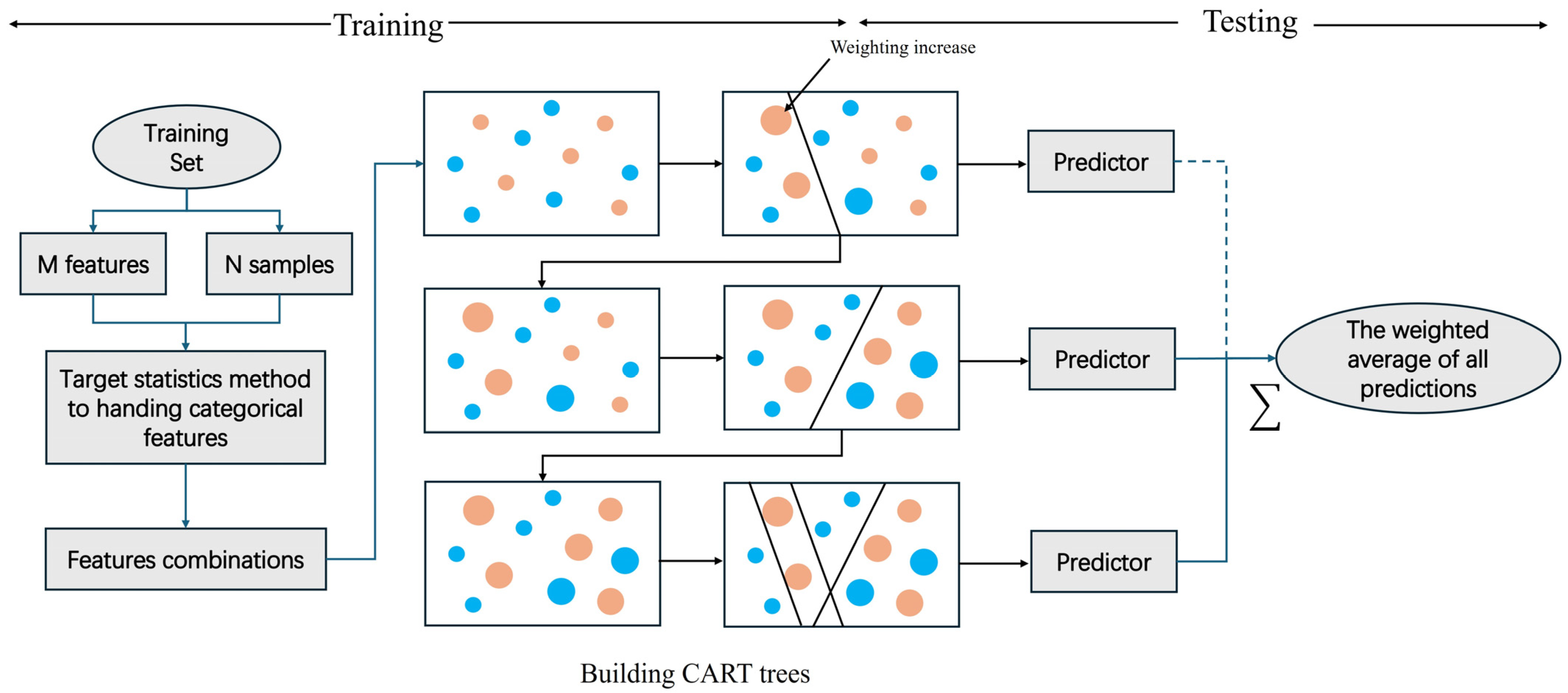
Feature engineering includes spectral-based information extraction and some classical mathematical transformations [44,45]. Local features include the Band Ratio Index (BRI) [46], Band Reciprocal Difference (BRD) [47], Normalized Difference Index (NDI) [15], and Three-Band Index (TBI) [48]. Local features constructed by band combination can better enhance water quality parameter signals [33]. Some scholars have proposed spectral combination forms suitable for different water quality parameters based on the absorption and scattering principles of water quality parameters. We traversed the Pearson correlation coefficients of the combination forms of each band, Chla and TSS and finally selected several combinations with correlations higher than 0.65 as local variables for feature engineering. The correlation screening results are shown in

Table 1. The highest correlation of each combination with Chla and TSS. The combination corresponding to bold font is used in this study.

Combination	Expression	Chla	Expression	TSS
BRI	${\displaystyle \frac{b10(681.25 \mathrm{n}\mathrm{m})}{b9(673.75 \mathrm{n}\mathrm{m})}}$	0.69	${\displaystyle \frac{b16(778.75 \mathrm{n}\mathrm{m})}{b5(510 \mathrm{n}\mathrm{m})}}$	0.73
BRD	${\displaystyle \frac{1}{b5(510 \mathrm{n}\mathrm{m})}}-{\displaystyle \frac{1}{b6(560 \mathrm{n}\mathrm{m})}}$	0.41	${\displaystyle \frac{1}{b2(412.5 \mathrm{n}\mathrm{m})}}-{\displaystyle \frac{1}{b17(865 \mathrm{n}\mathrm{m})}}$	0.32
NDI	${\displaystyle \frac{b10(681.25 \mathrm{n}\mathrm{m})-b9(673.75 \mathrm{n}\mathrm{m})}{b10(681.25 \mathrm{n}\mathrm{m})+b9(673.75 \mathrm{n}\mathrm{m})}}$	0.68	${\displaystyle \frac{b16(778.75 \mathrm{n}\mathrm{m})}{b4(490 \mathrm{n}\mathrm{m})}}$	0.70
TBI	${\displaystyle \frac{b7(620 \mathrm{n}\mathrm{m})+b11(708.75 \mathrm{n}\mathrm{m})}{b8(665 \mathrm{n}\mathrm{m})}}$	0.65	${\displaystyle \frac{b12(753.75 \mathrm{n}\mathrm{m})+b16(778.75 \mathrm{n}\mathrm{m})}{b5(510 \mathrm{n}\mathrm{m})}}$	0.72

. To avoid feature redundancy, we will not reuse combinations formed by the same bands. The correlation results between different band combinations and water quality elements are shown in Table 1. Based on the results, we finally selected the BRI consisting of b10 and b9 and the TBI combination consisting of b7, b8, and b11 as the local features for estimating Chla concentration, and we selected the BRI consisting of b16 and b5, the NDI consisting of b16 and b4, and the TBI consisted of b5, b12, and b16 as the local features for estimating the TSS concentration.

According to the results shown in Table 1, the best combination of BRI, NDI, and TBI has the best correlation with TSS, and the correlation is higher than 0.7, and the correlation with Chla has also reached a good 0.65 or above. From the perspective of the bands of the best combination, b4, b5, b12, and b16 are the best bands for TSS inversion, corresponding to the blue, green, and near-infrared ranges, respectively. Relevant studies have shown that when the TSS concentration of water increases, the transparency of the water decreases, and the reflection peak of the green-light band of the spectral curve moves toward the long-wave direction [49]. The interval composed of bands b4, b5, and b12 is exactly a reflection peak interval of high TSS concentration, and band b16 is the second reflection peak of the spectral curve under high TSS concentration; for Chla concentration, the five bands from b7 to b11 constitute the best band for inverting Chla, which is the green-light and red-light interval. In this interval, as the Chla concentration increases, the spectral curve often forms a second reflection peak, which can be used as a key feature for estimating Chla concentration.

However, it is obviously not enough to rely solely on band combinations as input features for building models. From the results of Section 3.1, the Chla and TSS content in water have a great influence on the spectral morphological characteristics. Under the influence of water quality parameters with different concentrations, the morphology of the spectrum is also different. This difference is mainly manifested in the rise and fall, convexity, and extreme values of the spectral curve. Based on constructing traditional band combination features, this study added spectral morphological characteristics and water body classification results as global features to improve the prediction ability of the model under different water quality parameter concentrations. The morphological features we selected include maximum reflectance (max_val), minimum reflectance (min_val), peak (peak_val), valley (valley_val), convexity, slope, rise (rise_amplitude) and fall (fall_amplitude). Here, we use the average value of the second-order derivative for convexity, and the rise and fall are expressed by the difference in the spectral curve.

3.2.2. CatBoost

Gradient boosting is a powerful machine learning algorithm that has been widely used in recent years in various prediction tasks, including water quality parameter inversion, and has achieved excellent results. However, the gradient boosting algorithm usually faces the following problem: the prediction model obtained by boosting depends on the training samples, which will cause the distribution of x in the training samples to shift compared with the test samples and ultimately lead to a prediction shift in the learning model. To solve the problem of target leakage and prediction shift, Yandex scientists proposed the CatBoost [50] algorithm in 2017. Its unique target statistical method [51] effectively enhances the robustness of the model, which is just suitable for small datasets such as water quality which are difficult to monitor and obtain. In addition, its powerful feature combination ability can deeply explore the interaction between features, which is particularly critical for understanding and predicting complex water quality characteristics. In this study, we therefore tried to use the CatBoost model to estimate Chla and TSS concentrations in the coastal waters of Fujian Province. The model structure is shown in Figure 6, which is modified from reference [51].

We first divided the 340 measured curves into a training set and a test set in a ratio of 7:3, extracted the global and local features of the spectrum on the training set and the testing set, respectively, set several important parameters of the model through the grid search method, and trained the model on the training set.

Table 2. Optimal values of CatBoost model parameters.

Parameters	Ranges	Optimal Values
iterations	[1, +∞]	1000
learning_rate	[0, 1]	0.01
depth	[1, +∞]	3
loss_function	RMSE, Logloss, MAPE, Poisson	RMSE
l2_leaf_reg	[1, +∞]	1

shows the optimal values of several parameters used in the study.

In terms of accuracy verification, we selected three evaluation indicators, R² (R-square), mean square error (MSE), and mean absolute percentage error (MAPE), to verify the accuracy on the test set. The formulas of the three indicators are shown below. In the formulas, $y_i$ represents the measured value, $\widehat{y}$ represents the model predicted value, $\overline{y}$ represents the measured average value, and n is the number of verification samples.

$$R^2=1-{\displaystyle \frac{{\displaystyle \sum _{i=1}^n{(y_i-{\hat{y}}_i)}^2}}{{\displaystyle \sum _{i=1}^n{(y_i-\overline{y})}^2}}}$$

(3)

$$MSE={\displaystyle \frac{{\displaystyle \sum _{i=1}^n{(y_i-\overline{y})}^2}}{n}}$$

(4)

$$MAPE={\displaystyle \sum _{i=1}^n\left|\frac{y_i-{\hat{y}}_i}{y_i}\right|}\times {\displaystyle \frac{100}{n}}$$

(5)

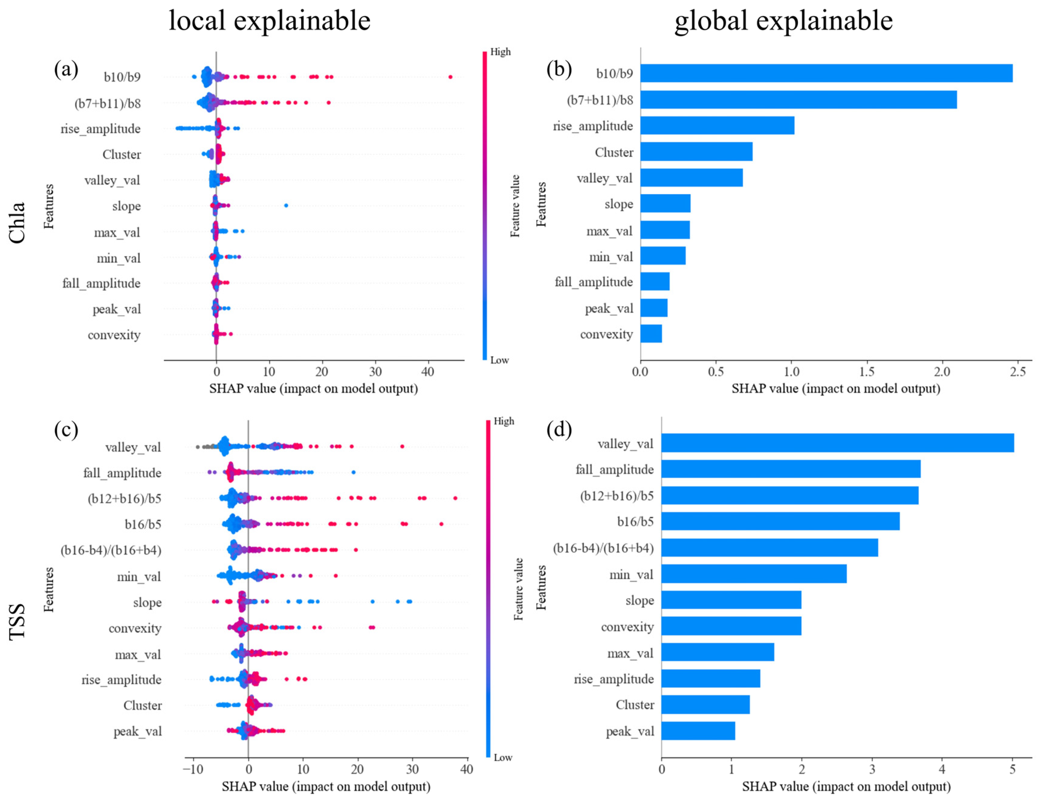
3.3. Model Interpretation by SHAP Model

After building the CatBoost model, we built a SHAP interpretability framework [52] for the model to identify the impact of relevant features on the model output. SHAP is a model-agnostic post hoc interpretability method that assigns each feature an importance value for a specific prediction. It has become one of the best methods for model interpretation [44,53]. The SHAP model uses the function G to determine the contribution of each feature variable to the model F. The function G is defined as shown in Equation (6) [54]:

$$G(z)={\phi }_0+{\displaystyle \sum _{i=1}^n{\phi }_i}{t}_i$$

(6)

where n represents the number of input features. For used features, the corresponding t value is 1, and for unused features, the corresponding t value is 0. ${\phi }_i$ represents the contribution of each feature to the model. The definition of contribution is as shown in Equation (7) [55]:

$${\phi }_i(F,x)={\displaystyle {\sum }_{t\subseteq x}\frac{\left|t\right|!(n-\left|t\right|-1)!}{n!}}\left[F(t)-F({\displaystyle \frac{n}{i}})\right]$$

(7)

4. Results and Discussion

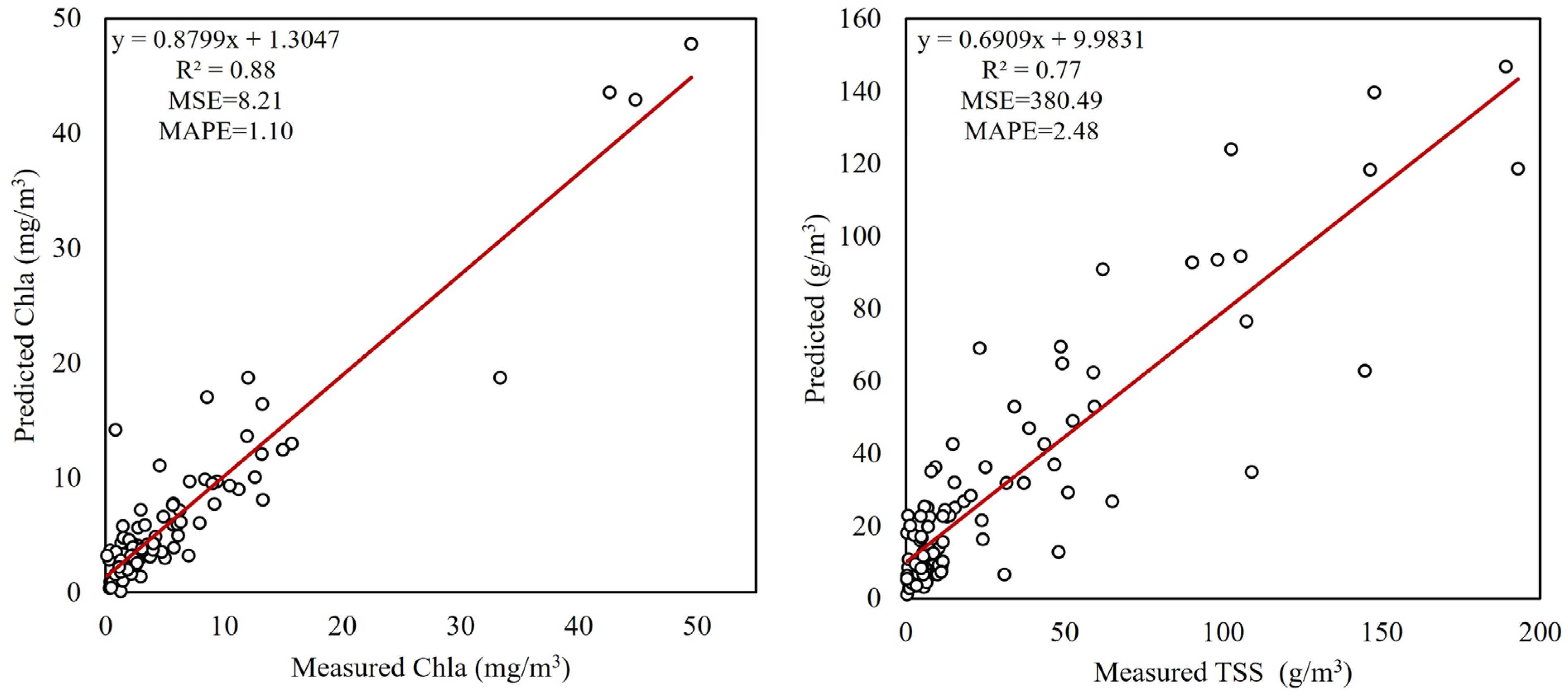
4.1. Model Accuracy and Explanation

Figure 7 shows the modeling results of CatBoost for Chla and TSS, respectively. The modeling results of Chla concentration (${\mathrm{R}}^2=0.88, \mathrm{MSE}=8.21, \mathrm{MAPE}=1.10$) are generally better than those of TSS concentration (${\mathrm{R}}^2=0.77, \mathrm{MSE}=380.49, \mathrm{MAPE}=2.48$). This conclusion is consistent with that reached by other studies [10,56,57]. We speculate that this may be related to the concentration range of Chla and TSS. For machine learning, the smaller the range of modeling target values, the higher the prediction accuracy. In this study, the distribution range of TSS values is larger than that of Chla values, which may cause the model to bring greater errors in predicting TSS values.

The model performs well at high Chla ($\mathrm{Chla}>40\mathrm{mg}/{\mathrm{m}}^3$) and low Chla concentrations ($\mathrm{Chla}<5\mathrm{mg}/{\mathrm{m}}^3$), but some high predictions appear in the medium concentration range; the model has an error of 20–30 g/m³ in high TSS concentrations, and most points in the low concentration range perform well. It is worth noting that the MSE of the modeling results of TSS shows a very large value compared with Chla, because MSE is more sensitive to outliers. Under a high TSS concentration, the prediction error will also increase, which ultimately leads to an increase in MSE. However, the MAPE of both remains in a relatively small range, so we believe that the model has a good inversion effect for Chla and TSS.

The modeling data, modeling results, and correlation matrix (Table S1) of the model (Figures S1 and S2) can be viewed by readers by downloading Supplementary Materials.

Figure 8 clearly shows the impact of each input feature on the model output. SHAP divides the impact of features on model output into local interpretability (Figure 8a,c) and global interpretability (Figure 8b,d).

In the Chla inversion results, b10/b9 and (b7 + b11)/b8 show a strong correlation, and the SHAP values of the red points are basically greater than zero, indicating that these two features play a positive role in the estimation of Chla concentration. In the case of high concentrations of Chla, the b10/b9 and (b7 + b11)/b8 of the image will also become higher accordingly. For the cluster and valley, when their eigenvalues are high, the SHAP values are distributed in the positive range of about 0, which means that although these two features are also relevant to the estimation of Chla, their contribution is not large. In addition, the maximum and minimum values of the spectral curve play a small negative correlation role in the estimation of Chla, because in the part where the SHAP value is greater than zero, their eigenvalues are basically blue, indicating low values. From the perspective of global interpretability, b10/b9, (b7 + b11)/b8, rise, and cluster are four important features that affect Chla estimation.

In the TSS inversion results, the valley value is a key factor in determining the TSS concentration. According to the results of Figure 6, the points with high valley values (red points in Figure 6) have positive SHAP values, and the points with low valley values (blue points in Figure 6) have mostly negative SHAP values, indicating that the valley value has a greater impact on the estimation of TSS concentration. When the TSS concentration increases, the valley value of the spectral curve becomes higher, and the curve is closer to the horizontal, which is the same as the water body classification result obtained in Section 3.1. For the rise and fall amplitude, the two are negatively correlated and positively correlated with the TSS concentration, respectively, and the decline amplitude has a greater impact on the TSS concentration estimation. In addition, the three local features (b12 + b16)/b5, b16/b5, and (b16 − b4)/(b16 + b4) also have a positive correlation with the TSS estimation that cannot be ignored, and the peak, slope, and cluster all have more or less influence on the TSS estimation. Compared with Chla, the features involved in TSS modeling have a more significant impact on the model.

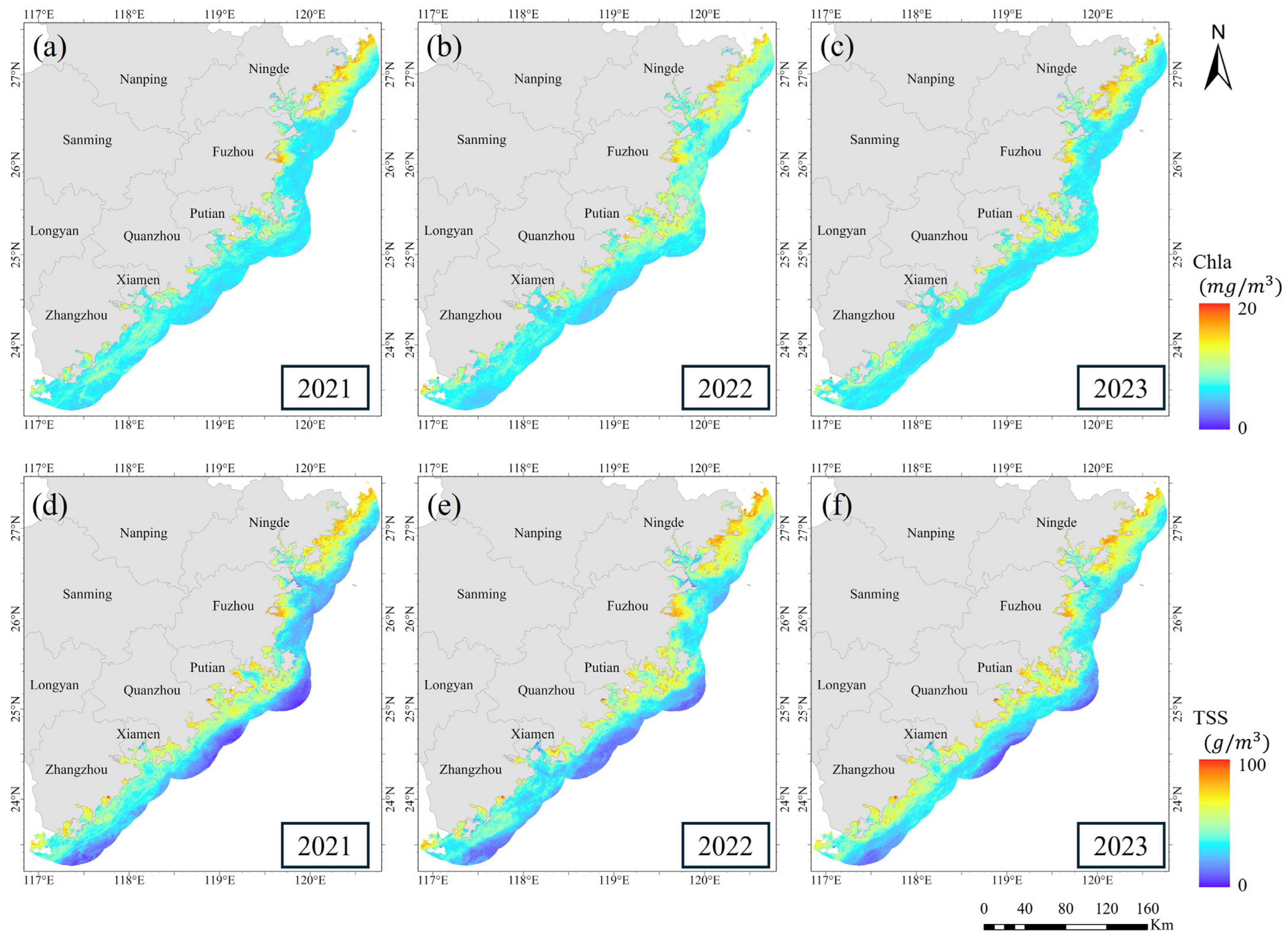
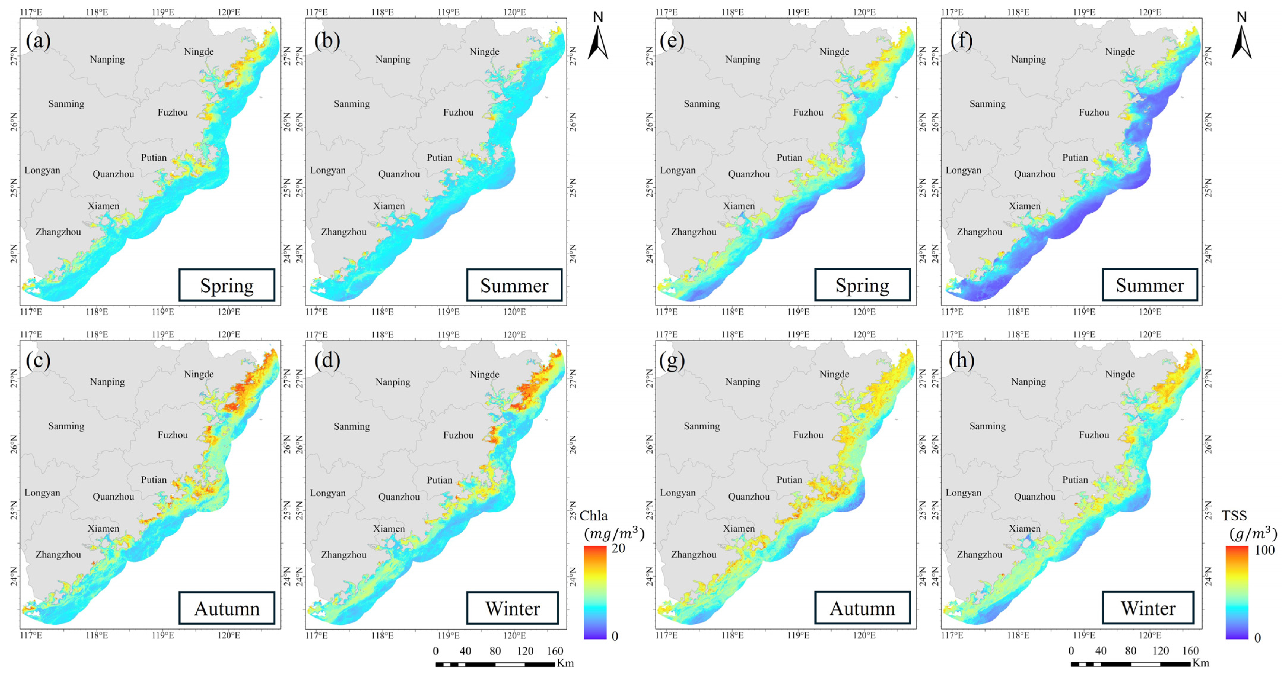
4.2. Chla and TSS Inversion Using OLCI

To understand the changing trends and spatiotemporal distribution of Chla and TSS at different times, we classified the inversion result maps by time, calculated their average inversion results from 2021 to 2023, and obtained six annual average inversion result maps of Chla and TSS in the coastal areas of Fujian Province based on OLCI-CatBoost. The results are shown in Figure 9.

From the perspective of temporal changes, the spatial distribution of Chla and TSS from 2021 to 2023 is basically the same, with little difference between different years, which basically conforms to the characteristics of high nearshore and low far shore. The average Chla concentration along the coast of the province in the past three years is about 7.7 mg/m³, and the TSS concentration is about 45 g/m³. The nearshore Chla concentration is concentrated at around 15 mg/m³, and the TSS concentration is around 60 g/m³. The far shore Chla concentration is basically around 5 mg/m³, and the TSS concentration is around 20 g/m³. This may be because the nearshore waters are affected by human activities [58], and the seawater environment is complex, especially the TSS concentration, which is also easily affected by surface runoff and coastal sediment alluvial deposits. The yellow area is larger than Chla and has a higher concentration.

From the perspective of spatial distribution, due to the excellent geographical conditions along the coast of Fujian Province, which has greatly promoted the development of the aquaculture industry, the high-value part of Chla in the province (that is, the yellow waters in the figure) is basically concentrated in the marine aquaculture area, such as the Sansha Bay in Ningde, the Xinghua Bay in Putian, Futou Bay in Zhangzhou, and Xiamen Bay in Xiamen. Among them, the Sansha Bay in Ningde and the Xinghua Bay in Putian are the two largest aquaculture bays in Fujian Province. The metabolic wastewater generated by aquaculture is easy to pollute the water quality, leading to higher algae reproduction. Simultaneously, there are also some industrial parks distributed along the coast of Ningde. The discharge of industrial wastewater may also lead to the eutrophication of coastal waters [59]. These factors work together to eventually increase the Chla concentration in the Ningde and Putian waters.

In addition to aquaculture and industrial activities, the river runoff into the sea is also an important factor causing the increase in TSS and Chla concentrations [60]. The eastern sea area of Fuzhou is a typical river estuary area. As the largest river in Fujian Province, there are many residential and industrial areas along the Minjiang River. At the same time, the tributaries that flow into the Minjiang River also carry a large amount of suspended sediment and pollutants, which eventually accumulate and precipitate downstream at the estuary, resulting in high Chla and TSS concentrations in the area.

To further understand the spatial distribution characteristics of Chla and TSS concentrations in different seasons, we also classified the three-year inversion results according to different seasons based on time and then calculated the average value. The results are shown in Figure 10.

It can be seen that there are significant seasonal differences between Chla and TSS. According to

Table 3. Chla and TSS statistical values in different seasons.

Factor		Spring	Summer	Autumn	Winter
Chla (mg/m3)	Average value	7.93	6.75	9.31	8.65
	Standard deviation	2.61	1.81	3.67	3.45
TSS (g/m3)	Average value	46.45	35.55	56.85	51.56
	Standard deviation	13.75	14.59	14.30	13.67

, the average concentrations of Chla and TSS reach their highest in autumn and winter and the lowest in summer. This seasonal difference may be related to the climate characteristics [61] and marine aquaculture schedule in Fujian Province. The period from June to September in Fujian Province is characterized by high temperatures and abundant rainfall, which increases surface runoff and dilutes pollutants in the water. Currently, aquaculture in Fujian Province is under a fishing ban period (usually starting from May 1st and lasting for three and a half months), and there has been a decrease in offshore aquaculture operations. This has resulted in lower concentrations of Chla and TSS along the coast in summer, with an even distribution of values and fewer occurrences of extremely high values. During the autumn and winter seasons, there is less rainfall in Fujian Province, and the coastal seawater mobility weakens. This is also the harvest time for aquaculture in Fujian Province, and the number of offshore operations increases. Due to both natural and human factors, the Chla and TSS concentrations in autumn and winter are higher than usual.

5. Conclusions

Our research established a new remote sensing inversion method for Chla and TSS water quality parameters, considering the morphological characteristics of spectral curves combined with OLCI sensors to capture the spectral characteristics of Chla and TSS along the coast of Fujian Province to estimate the concentrations of Chla and TSS along the coast of Fujian Province in recent years. The research results indicate the following:

(1) Different types of water bodies in the coastal waters of Fujian Province have distinct shape characteristics, ranging from the green-light band to the near-infrared band. There are significant differences between water bodies with different concentrations of Chla and TSS.

(2) Comparing different combinations of spectral features, we found that BRI, NDI, and TBI show strong sensitivity to changes in Chla and TSS concentrations. The CatBoost prediction model constructed by combining these combinations with the classification features of spectral curves achieved a prediction R² of 0.88 for Chla concentration and 0.77 for TSS concentration, and other evaluation indicators of the model were also at good levels.

(3) We analyzed the impact of different features on the output of model prediction results by the SHAP model and found that specific band combinations (such as BRI, NDI) and the concavity and convexity of spectral curves can have a strong influence on the model’s prediction results.

(4) We used the constructed model to predict the concentrations of Chla and TSS in the coastal waters of Fujian Province from 2021 to 2023 and conducted spatiotemporal analysis. The results indicate that there have been no significant changes in the annual average concentrations of Chla and TSS in recent years, but there are significant seasonal differences which may be related to the climate characteristics and aquaculture operation patterns along the coast of Fujian Province.

However, there are still some deficiencies in our current research. First, the modeling data we used comes from the GLORIA public dataset, and there is a lack of datasets in the study area for verification. At the same time, the analysis of factors affecting the changes in the water environment in Fujian Province is still theoretical and speculative. Therefore, in future research, we hope to accurately analyze the influencing factors that cause changes in chlorophyll-a and total suspended particulate matter concentrations, and further improve the prediction ability of the model. In addition, if we can obtain measured water quality data from the coastal areas of Fujian Province, we will also try to include it in our research scope.

References

1. Ward, N.D.; Megonigal, J.P.; Bond-Lamberty, B.; Bailey, V.L.; Butman, D.; Canuel, E.A.; Diefenderfer, H.; Ganju, N.K.; Goñi, M.A.; Graham, E.B. Representing the function and sensitivity of coastal interfaces in Earth system models. Nat. Commun. 2020, 11, 2458. [Google Scholar] [CrossRef] [PubMed]
2. Zhai, T.; Wang, J.; Fang, Y.; Qin, Y.; Huang, L.; Chen, Y. Assessing ecological risks caused by human activities in rapid urbanization coastal areas: Towards an integrated approach to determining key areas of terrestrial-oceanic ecosystems preservation and restoration. Sci. Total Environ. 2020, 708, 135153. [Google Scholar] [CrossRef]
3. Yu, J.; Zhou, D.; Yu, M.; Yang, J.; Li, Y.; Guan, B.; Wang, X.; Zhan, C.; Wang, Z.; Qu, F. Environmental threats induced heavy ecological burdens on the coastal zone of the Bohai Sea, China. Sci. Total Environ. 2021, 765, 142694. [Google Scholar] [CrossRef] [PubMed]
4. Wang, H.; Wang, G.; Gu, W. Macroalgal blooms caused by marine nutrient changes resulting from human activities. J. Appl. Ecol. 2020, 57, 766–776. [Google Scholar] [CrossRef]
5. Ahmad, A.; Abdullah, S.R.S.; Hasan, H.A.; Othman, A.R.; Ismail, N.I. Aquaculture industry: Supply and demand, best practices, effluent and its current issues and treatment technology. J. Environ. Manag. 2021, 287, 112271. [Google Scholar] [CrossRef]
6. Trottet, A.; George, C.; Drillet, G.; Lauro, F.M. Aquaculture in coastal urbanized areas: A comparative review of the challenges posed by Harmful Algal Blooms. Crit. Rev. Environ. Sci. Technol. 2022, 52, 2888–2929. [Google Scholar] [CrossRef]
7. Lu, Y.; Yuan, J.; Lu, X.; Su, C.; Zhang, Y.; Wang, C.; Cao, X.; Li, Q.; Su, J.; Ittekkot, V. Major threats of pollution and climate change to global coastal ecosystems and enhanced management for sustainability. Environ. Pollut. 2018, 239, 670–680. [Google Scholar] [CrossRef]
8. Cui, T.; Zhang, J.; Wang, K.; Wei, J.; Mu, B.; Ma, Y.; Zhu, J.; Liu, R.; Chen, X. Remote sensing of chlorophyll a concentration in turbid coastal waters based on a global optical water classification system. ISPRS J. Photogramm. Remote Sens. 2020, 163, 187–201. [Google Scholar] [CrossRef]
9. Jiang, D.; Matsushita, B.; Pahlevan, N.; Gurlin, D.; Lehmann, M.K.; Fichot, C.G.; Schalles, J.; Loisel, H.; Binding, C.; Zhang, Y. Remotely estimating total suspended solids concentration in clear to extremely turbid waters using a novel semi-analytical method. Remote Sens. Environ. 2021, 258, 112386. [Google Scholar] [CrossRef]
10. Saberioon, M.; Brom, J.; Nedbal, V.; Souček, P.; Císař, P. Chlorophyll-a and total suspended solids retrieval and mapping using Sentinel-2A and machine learning for inland waters. Ecol. Indic. 2020, 113, 106236. [Google Scholar] [CrossRef]
11. Brezonik, P.L.; Bouchard, R.W., Jr.; Finlay, J.C.; Griffin, C.G.; Olmanson, L.G.; Anderson, J.P.; Arnold, W.A.; Hozalski, R. Color, chlorophyll a, and suspended solids effects on Secchi depth in lakes: Implications for trophic state assessment. Ecol. Appl. 2019, 29, e01871. [Google Scholar] [CrossRef]
12. Pahlevan, N.; Smith, B.; Alikas, K.; Anstee, J.; Barbosa, C.; Binding, C.; Bresciani, M.; Cremella, B.; Giardino, C.; Gurlin, D. Simultaneous retrieval of selected optical water quality indicators from Landsat-8, Sentinel-2, and Sentinel-3. Remote Sens. Environ. 2022, 270, 112860. [Google Scholar] [CrossRef]
13. Chen, J.; Chen, S.; Fu, R.; Li, D.; Jiang, H.; Wang, C.; Peng, Y.; Jia, K.; Hicks, B.J. Remote sensing big data for water environment monitoring: Current status, challenges, and future prospects. Earth’s Future 2022, 10, e2021EF002289. [Google Scholar] [CrossRef]
14. Kolluru, S.; Tiwari, S.P. Modeling ocean surface chlorophyll-a concentration from ocean color remote sensing reflectance in global waters using machine learning. Sci. Total Environ. 2022, 844, 157191. [Google Scholar] [CrossRef] [PubMed]
15. Mishra, S.; Mishra, D.R. Normalized difference chlorophyll index: A novel model for remote estimation of chlorophyll-a concentration in turbid productive waters. Remote Sens. Environ. 2012, 117, 394–406. [Google Scholar] [CrossRef]
16. Huang, C.; Zou, J.; Li, Y.; Yang, H.; Shi, K.; Li, J.; Wang, Y.; Chena, X.; Zheng, F. Assessment of NIR-red algorithms for observation of chlorophyll-a in highly turbid inland waters in China. ISPRS J. Photogramm. Remote Sens. 2014, 93, 29–39. [Google Scholar] [CrossRef]
17. Gurlin, D.; Gitelson, A.A.; Moses, W.J. Remote estimation of chl-a concentration in turbid productive waters—Return to a simple two-band NIR-red model? Remote Sens. Environ. 2011, 115, 3479–3490. [Google Scholar] [CrossRef]
18. Chen, S.; Fang, L.; Li, H.; Chen, W.; Huang, W. Evaluation of a three-band model for estimating chlorophyll-a concentration in tidal reaches of the Pearl River Estuary, China. ISPRS J. Photogramm. Remote Sens. 2011, 66, 356–364. [Google Scholar] [CrossRef]
19. Zhao, J.; Zhang, F.; Chen, S.; Wang, C.; Chen, J.; Zhou, H.; Xue, Y. Remote sensing evaluation of total suspended solids dynamic with Markov model: A case study of inland reservoir across administrative boundary in South China. Sensors 2020, 20, 6911. [Google Scholar] [CrossRef]
20. Zhang, Y.; Zhang, Y.; Shi, K.; Zha, Y.; Zhou, Y.; Liu, M. A Landsat 8 OLI-based, semianalytical model for estimating the total suspended matter concentration in the slightly turbid Xin’anjiang Reservoir (China). IEEE J. Sel. Top. Appl. Earth Obs. Remote Sens. 2016, 9, 398–413. [Google Scholar] [CrossRef]
21. Binh, N.A.; Hoa, P.V.; Thao, G.T.P.; Duan, H.D.; Thu, P.M. Evaluation of Chlorophyll-a estimation using Sentinel 3 based on various algorithms in southern coastal Vietnam. Int. J. Appl. Earth Obs. Geoinf. 2022, 112, 11. [Google Scholar] [CrossRef]
22. Le, C.; Li, Y.; Zha, Y.; Sun, D.; Huang, C.; Lu, H. A four-band semi-analytical model for estimating chlorophyll a in highly turbid lakes: The case of Taihu Lake, China. Remote Sens. Environ. 2009, 113, 1175–1182. [Google Scholar] [CrossRef]
23. Sun, X.; Zhang, Y.; Shi, K.; Zhang, Y.; Li, N.; Wang, W.; Huang, X.; Qin, B. Monitoring water quality using proximal remote sensing technology. Sci. Total Environ. 2022, 803, 149805. [Google Scholar] [CrossRef] [PubMed]
24. Chen, P.; Wang, B.; Wu, Y.; Wang, Q.; Huang, Z.; Wang, C. Urban river water quality monitoring based on self-optimizing machine learning method using multi-source remote sensing data. Ecol. Indic. 2023, 146, 109750. [Google Scholar] [CrossRef]
25. Yang, H.; Du, Y.; Zhao, H.; Chen, F. Water quality Chl-a inversion based on spatio-temporal fusion and convolutional neural network. Remote Sens. 2022, 14, 1267. [Google Scholar] [CrossRef]
26. Wen, Z.; Wang, Q.; Ma, Y.; Jacinthe, P.A.; Liu, G.; Li, S.; Shang, Y.; Tao, H.; Fang, C.; Lyu, L. Remote estimates of suspended particulate matter in global lakes using machine learning models. Int. Soil Water Conserv. Res. 2024, 12, 200–216. [Google Scholar] [CrossRef]
27. Liu, Y.; Zhang, C.; Chen, X. Knowledge-guided mixture density network for chlorophyll-a retrieval and associated pixel-by-pixel uncertainty assessment in optically variable inland waters. Sci. Total Environ. 2024, 919, 170843. [Google Scholar] [CrossRef]
28. Zhong, S.; Zhang, K.; Bagheri, M.; Burken, J.G.; Gu, A.; Li, B.; Ma, X.; Marrone, B.L.; Ren, Z.J.; Schrier, J.; et al. Machine learning: New ideas and tools in environmental science and engineering. Environ. Sci. 2021, 55, 12741–12754. [Google Scholar] [CrossRef]
29. Tang, C.; Jiang, X.; Li, G.; Lu, D. Developing a New Method to Rapidly Map Eucalyptus Distribution in Subtropical Regions Using Sentinel-2 Imagery. Forests 2024, 15, 1799. [Google Scholar] [CrossRef]
30. Joshi, N.; Park, J.; Zhao, K.; Londo, A.; Khanal, S. Monitoring Harmful Algal Blooms and Water Quality Using Sentinel-3 OLCI Satellite Imagery with Machine Learning. Remote Sens. 2024, 16, 2444. [Google Scholar] [CrossRef]
31. Brockmann, C.; Doerffer, R.; Peters, M.; Kerstin, S.; Embacher, S.; Ruescas, A. Evolution of the C2RCC neural network for Sentinel 2 and 3 for the retrieval of ocean colour products in normal and extreme optically complex waters. In Proceedings of the Living Planet Symposium, Prague, Czech Republic, 9 May 2016; p. 54. [Google Scholar]
32. Doerffer, R.; Schiller, H. The MERIS Case 2 water algorithm. Int. J. Remote Sens. 2007, 28, 517–535. [Google Scholar] [CrossRef]
33. Su, H.; Lu, X.; Chen, Z.; Zhang, H.; Lu, W.; Wu, W. Estimating coastal chlorophyll-a concentration from time-series OLCI data based on machine learning. Remote Sens. 2021, 13, 576. [Google Scholar] [CrossRef]
34. Giannini, F.; Hunt, B.P.; Jacoby, D.; Costa, M. Performance of OLCI Sentinel-3A satellite in the Northeast Pacific coastal waters. Remote Sens. Environ. 2021, 256, 112317. [Google Scholar] [CrossRef]
35. Lehmann, M.K.; Gurlin, D.; Pahlevan, N.; Alikas, K.; Anstee, J.; Balasubramanian, S.V.; Barbosa, C.C.F.; Binding, C.; Bracher, A.; Bresciani, M.; et al. GLORIA-A globally representative hyperspectral in situ dataset for optical sensing of water quality. Sci. Data 2023, 10, 14. [Google Scholar] [CrossRef]
36. Luo, W.; Li, R.; Shen, F.; Liu, J. HY-1C/D CZI image atmospheric correction and quantifying suspended particulate matter. Remote Sens. 2023, 15, 386. [Google Scholar] [CrossRef]
37. Cai, X.; Li, Y.; Bi, S.; Lei, S.; Xu, J.; Wang, H.; Dong, X.; Li, J.; Zeng, S.; Lyu, H. Urban water quality assessment based on remote sensing reflectance optical classification. Remote Sens. 2021, 13, 4047. [Google Scholar] [CrossRef]
38. Li, L.; Gu, M.; Gong, C.; Hu, Y.; Wang, X.; Yang, Z.; He, Z. An advanced remote sensing retrieval method for urban non-optically active water quality parameters: An example from Shanghai. Sci. Total Environ. 2023, 880, 163389. [Google Scholar] [CrossRef]
39. Waleed, M.; Um, T.-W.; Khan, A.; Khan, U. Automatic detection system of olive trees using improved K-means algorithm. Remote Sens. 2020, 12, 760. [Google Scholar] [CrossRef]
40. Abbas, A.W.; Minallh, N.; Ahmad, N.; Abid, S.A.R.; Khan, M.A.A. K-Means and ISODATA clustering algorithms for landcover classification using remote sensing. Sindh Univ. Res. J.-SURJ 2016, 48, 315–318. [Google Scholar]
41. Ren, Z.; Sun, L.; Zhai, Q. Improved k-means and spectral matching for hyperspectral mineral mapping. Int. J. Appl. Earth Obs. Geoinf. 2020, 91, 102154. [Google Scholar] [CrossRef]
42. Ackermann, M.R.; Blömer, J.; Kuntze, D.; Sohler, C. Analysis of agglomerative clustering. Algorithmica 2014, 69, 184–215. [Google Scholar] [CrossRef]
43. Xia, P.; Zhang, L.; Li, F. Learning similarity with cosine similarity ensemble. Inf. Sci. 2015, 307, 39–52. [Google Scholar] [CrossRef]
44. Zhu, L.; Cui, T.; Runa, A.; Pan, X.; Zhao, W.; Xiang, J.; Cao, M. Robust remote sensing retrieval of key eutrophication indicators in coastal waters based on explainable machine learning. ISPRS J. Photogramm. Remote Sens. 2024, 211, 262–280. [Google Scholar] [CrossRef]
45. Guo, H.; Tian, S.; Huang, J.J.; Zhu, X.; Wang, B.; Zhang, Z. Performance of deep learning in mapping water quality of Lake Simcoe with long-term Landsat archive. ISPRS J. Photogramm. Remote Sens. 2022, 183, 451–469. [Google Scholar] [CrossRef]
46. Yang, Z.; Reiter, M.; Munyei, N. Estimation of chlorophyll-a concentrations in diverse water bodies using ratio-based NIR/Red indices. Remote Sens. Appl. Soc. Environ. 2017, 6, 52–58. [Google Scholar] [CrossRef]
47. Escoto, J.; Blanco, A.; Argamosa, R.; Medina, J. Pasig river water quality estimation using an empirical ordinary least squares regression model of Sentinel-2 satellite images. Int. Arch. Photogramm. Remote Sens. Spat. Inf. Sci. 2021, 46, 161–168. [Google Scholar] [CrossRef]
48. Elsayed, S.; Gad, M.; Farouk, M.; Saleh, A.H.; Hussein, H.; Elmetwalli, A.H.; Elsherbiny, O.; Moghanm, F.S.; Moustapha, M.E.; Taher, M.A. Using optimized two and three-band spectral indices and multivariate models to assess some water quality indicators of Qaroun Lake in Egypt. Sustainability 2021, 13, 10408. [Google Scholar] [CrossRef]
49. Novo, E.M.L.M.; Steffen, C.A.; Braga, C.Z.F. Results of a laboratory experiment relating spectral reflectance to total suspended solids. Remote Sens. Environ. 1991, 36, 67–72. [Google Scholar] [CrossRef]
50. Prokhorenkova, L.; Gusev, G.; Vorobev, A.; Dorogush, A.V.; Gulin, A. CatBoost: Unbiased boosting with categorical features. Adv. Neural Inf. Process. Syst. 2018, 31, 6637–6647. [Google Scholar]
51. Huang, G.; Wu, L.; Ma, X.; Zhang, W.; Fan, J.; Yu, X.; Zeng, W.; Zhou, H. Evaluation of CatBoost method for prediction of reference evapotranspiration in humid regions. J. Hydrol. 2019, 574, 1029–1041. [Google Scholar] [CrossRef]
52. Lundberg, S.M.; Lee, S.-I. A unified approach to interpreting model predictions. Adv. Neural Inf. Process. Syst. 2017, 30, 4765–4774. [Google Scholar]
53. Yang, W.; Fu, B.; Li, S.; Lao, Z.; Deng, T.; He, W.; He, H.; Chen, Z. Monitoring multi-water quality of internationally important karst wetland through deep learning, multi-sensor and multi-platform remote sensing images: A case study of Guilin, China. Ecol. Indic. 2023, 154, 110755. [Google Scholar] [CrossRef]
54. Kim, Y.; Kim, Y. Explainable heat-related mortality with random forest and SHapley Additive exPlanations (SHAP) models. Sustain. Cities Soc. 2022, 79, 103677. [Google Scholar] [CrossRef]
55. Pelegrina, G.D.; Duarte, L.T.; Grabisch, M. A k-additive Choquet integral-based approach to approximate the SHAP values for local interpretability in machine learning. Artif. Intell. 2023, 325, 104014. [Google Scholar] [CrossRef]
56. Xiao, Y.; Chen, J.; Xu, Y.; Guo, S.; Nie, X.; Guo, Y.; Li, X.; Hao, F.; Fu, H.Y. Monitoring of chlorophyll-a and suspended sediment concentrations in optically complex inland rivers using multisource remote sensing measurements. Ecol. Indic. 2023, 155, 111041. [Google Scholar] [CrossRef]
57. O’Shea, R.E.; Pahlevan, N.; Smith, B.; Boss, E.; Gurlin, D.; Alikas, K.; Kangro, K.; Kudela, R.M.; Vaičiūtė, D. A hyperspectral inversion framework for estimating absorbing inherent optical properties and biogeochemical parameters in inland and coastal waters. Remote Sens. Environ. 2023, 295, 113706. [Google Scholar] [CrossRef]
58. Tian, K.; Wu, Q.; Liu, P.; Hu, W.; Huang, B.; Shi, B.; Zhou, Y.; Kwon, B.-O.; Choi, K.; Ryu, J. Ecological risk assessment of heavy metals in sediments and water from the coastal areas of the Bohai Sea and the Yellow Sea. Environ. Int. 2020, 136, 105512. [Google Scholar] [CrossRef]
59. Jiang, L.; Lu, X.; Wang, G.; Peng, M.; Wei, A.; Zhao, Y.; Soetaert, K. Unraveling seasonal and interannual nutrient variability shows exceptionally high human impact in eutrophic coastal waters. Limnol. Oceanogr. 2023, 68, 1161–1171. [Google Scholar] [CrossRef]
60. Zhu, X.; Guo, H.; Huang, J.J.; Tian, S.; Zhang, Z. A hybrid decomposition and Machine learning model for forecasting Chlorophyll-a and total nitrogen concentration in coastal waters. J. Hydrol. 2023, 619, 129207. [Google Scholar] [CrossRef]
61. Cao, Z.; Duan, H.; Feng, L.; Ma, R.; Xue, K. Climate-and human-induced changes in suspended particulate matter over Lake Hongze on short and long timescales. Remote Sens. Environ. 2017, 192, 98–113. [Google Scholar] [CrossRef]
Figure 1. Location of Fujian Province and study area.
Water 16 03615 g001
Figure 2. GLORIA data points used in the study.
Water 16 03615 g002
Figure 3. Research flow chart.
Water 16 03615 g003
Figure 4. (a) Average spectral curve of each category. (b) Chla concentration distribution of different clusters. (c) TSS concentration distribution of different clusters.
Water 16 03615 g004
Figure 5. Clustering results of coastal water bodies in Fujian Province in different seasons. Figures (ad) show the average maps of water classification for spring, summer, autumn, and winter.
Water 16 03615 g005
Figure 6. The structure of the CatBoost algorithm.
Water 16 03615 g006
Figure 7. Prediction results of the CatBoost model on the test set (the red line is the trend line).
Water 16 03615 g007
Figure 8. Interpretability results of spectral features for CatBoost inversion model of Chla and TSS by SHAP analysis. Figure (a) shows the local explainable results of Chla, Figure (b) shows the global explainable results of Chla, Figure (c) shows the local explainable results of TSS, and Figure (d) shows the global explainable results of TSS. (In the left column chart, one dot represents a sample, where warmer colors indicate larger values of the feature, and vice versa. The wider the distribution of SHAP values for a feature, the larger its global SHAP value, indicating that the feature has a greater impact on the model. In the right column chart, the white numbers on the blue bar represent the average absolute SHAP value [44].)
Water 16 03615 g008
Figure 9. Annual average concentration distribution map of Chla and TSS along the coast of Fujian Province from 2021 to 2023. (ac) is the average concentration of Chla, and (df) is the average concentration of TSS.
Water 16 03615 g009
Figure 10. Average Chla and TSS concentration values in different seasons along the coast of Fujian Province from 2021 to 2023. The four graphs on the left (ad) show the average concentration of Chla, while the four graphs on the right (eh) show the average concentration of TSS.
Water 16 03615 g010