Article

A Dam Safety State Prediction and Analysis Method Based on EMD-SSA-LSTM

1
Nanjing Hydraulic Research Institute, Nanjing 210029, China
2
The National Key Laboratory of Water Disaster Prevention, Nanjing 210029, China
*
Author to whom correspondence should be addressed.
Water 2024, 16(3), 395; https://doi.org/10.3390/w16030395
Submission received: 13 December 2023 / Revised: 14 January 2024 / Accepted: 23 January 2024 / Published: 24 January 2024
(This article belongs to the Special Issue Safety Evaluation of Dam and Geotechnical Engineering, Volume II)

Abstract

:
The safety monitoring information of the dam is an indicator reflecting the operational status of the dam. It is a crucial source for analyzing and assessing the safety state of reservoir dams, possessing strong real-time capabilities to detect anomalies in the dam at the earliest possible time. When using neural networks for predicting and warning dam safety monitoring data, there are issues such as redundant model parameters, difficulty in tuning, and long computation times. This study addresses real-time dam safety warning issues by first employing the Empirical Mode Decomposition (EMD) method to decompose the effective time-dependent factors and construct a dam in a service state analysis model; it also establishes a multi-dimensional time series analysis equation for dam seepage monitoring. Simultaneously, by combining the Sparrow Optimization Algorithm to optimize the LSTM neural network computation process, it reduces the complexity of model parameter selection. The method is compared to other approaches such as RNN, GRU, BP neural networks, and multivariate linear regression, demonstrating high practicality. It can serve as a valuable reference for reservoir dam state prediction and engineering operation management.

1. Introduction

The analysis of the safety state of a dam includes two main components: numerical calculations and the analysis of monitoring data. Dam safety monitoring is crucial for understanding the operational status and trends of the dam. It is an essential measure to ensure the safe operation of the dam, serving as a means to verify design outcomes, inspect construction quality, and comprehend the variations in various parameters of the dam [1,2]. Dam safety monitoring possesses strong real-time capabilities, enabling the prompt detection of anomalies in the dam. It facilitates the rapid assessment and monitoring of the dam’s safety operation status, providing insights into the working conditions and variations of hydraulic structures under adverse loads and various influencing factors [3,4,5]. By analyzing monitoring data, one can make correct judgments and evaluations regarding the safety level of the engineering structure, thereby providing a basis for the safe operation of reservoir dams [6]. It is beneficial for timely assessment and response to emergencies, offering scientific and timely data information for on-site inspections. This approach overcomes the uncertainty consequences that may arise from a delayed response to external anomalies in the dam, which might occur when relying solely on manual intermittent inspections [7,8].
Dam warnings for reservoirs primarily rely on systematic mechanisms for early warning [9]. This involves learning and summarizing the evolving patterns of measured data through empirical data analysis [10,11,12]. By establishing appropriate monitoring data prediction models, it is possible to simulate and predict the dam’s own behavior, providing proactive measures for the safe operation of the dam [13,14,15,16]. The research on monitoring models primarily focuses on three main aspects: (1) mathematical relationships between dependent and independent variables; (2) rational selection of independent variables and addressing multicollinearity; and (3) improving model accuracy, robustness, and generalization.
Currently, monitoring data prediction methods can be broadly categorized into two main types: statistical methods and time series methods [17,18,19]. Statistical methods aim to establish functional relationships between monitoring effects (such as displacement, seepage, uplift pressure, piezometric water level, etc.) and independent variables (such as reservoir water level, temperature, time, etc.) [20,21]. Therefore, mathematical methods such as multivariate linear regression, stepwise regression, principal component regression, partial least squares regression, and others have been applied sequentially to establish dam safety warning models. Researchers have explored various theoretical and methodological aspects related to long-term deformation safety monitoring and warnings for high concrete dams [22,23]. M. Tatin et al., proposed a statistical model accounting for the water temperature profile, which can describe the effects of both profiles of the water temperature and the dam thickness on dam displacements [24]. Sevieri et al., proposed a framework for dynamic monitoring of structural health of concrete gravity dams in a Bayesian environment by detecting damage and reducing the uncertainty of predicting dam structural behavior, so as to improve the reliability of the structural health monitoring system [25]. Wang et al., using the spatial clustering based on incremental distance, established a spatially correlated coupled support vector machine (SVM) model to predict the displacement of dams [26]. Li et al., proposed a separation modeling technique based on ICEEMDAN and cluster analysis by providing temperature components through theoretical inference and parameter optimization. The proposed model has high accuracy, credibility, and interpretability [27]. Luong Ha Nguyen proposed an anomaly detection method, which is tackled by combining a Rao-Blackwellized particle filter (RBPF) with the Bayesian dynamic linear models (BDLMs), to be capable of performing real-time analysis [28]. Shao et al., proposed an IVM and RF algorithm based on adaptive optimization to predict the deformation of concrete dams [29]. Lei et al., used principal component analysis (PCA) to reconstruct the features of an equidimensional mapping, integrated the dam displacement monitoring models of support vector regression (SVR), used MLP neural network (MLP) and Gaussian process regression (GPR), and proposed a superposed heterogeneous integration model of static and dynamic monitoring [30]. Su et al., using a combined support vector machine, chaos theory, and a particle swarm optimization algorithm, proposed a method to optimize the input and parameters of the prediction model and established a dam safety prediction model [31]. H. H. Yavaşoğlu et al., through a detailed analysis of the deformation and strain of the Ataturk Dam in Turkey, believe that using data from different technologies to monitor and diagnose the dam structure is an indispensable method [32]. With the advancement of computer technology, machine learning techniques have gradually been applied to the analysis of dam safety monitoring data [33,34]. Intelligent monitoring models such as random forests, neural networks, extreme learning machines, and others have shown significant improvements in prediction accuracy compared to traditional models, enabling more accurate predictions of dam safety states [35,36,37,38].
This study begins by employing the Empirical Mode Decomposition (EMD) algorithm to extract and analyze the time-effect components in the measured data of dam safety states. It establishes a response function for the time-effect components and constructs a multivariate time series analysis model that considers variables such as water pressure, temperature, rainfall, and time-effect. Recognizing the challenges of optimizing parameters in the use of LSTM neural networks for predicting dam safety states, the study selects iteration times, the number of nodes in two hidden layers, and the number of training samples in the network architecture as optimization targets. It employs the Sparrow Search Algorithm for intelligent parameter selection, aiming to enhance the intelligence and robustness of the predictive model. In the end, the study compares the predictive performance of the constructed EMD-SSA-LSTM dam safety state prediction model with GPU, RNN, BP neural networks, and the commonly used multivariate linear regression. The goal is to validate the superiority of the proposed model in predicting the safety state of the dam.

2. The Selection of Factors Affecting the Service State of the Dam Is Diverse

2.1. Empirical Mode Decomposition of Aging Factors

The mathematical model during operation includes various components of causal factors (such as pressure components, temperature components, and aging components) [39,40]. Among them, the variation in the aging component is an important basis for evaluating the normality of the response quantity, and the reasons for abnormal changes need to be identified. Empirical Mode Decomposition (EMD) is a novel adaptive signal time-frequency processing method proposed by N. E. Huang, especially suitable for the analysis and processing of nonlinear and non-stationary signals [41,42].
This method creatively introduces the concept of Intrinsic Mode Functions (IMF) and proves the theoretical decomposition of any signal into a series of intrinsic mode functions. EMD is based on the assumption that any signal is composed of Intrinsic Mode Functions (IMF), where the components can be linear or nonlinear; furthermore, a signal can be composed of many components of intrinsic modes, and if the components overlap with each other, a composite signal is formed [43].
IMF components must satisfy the following two conditions:
(1)
The number of zero crossings and extrema is the same throughout the entire data set, or the two differ by at most one.
(2)
The sum of the mean of the upper and lower envelopes composed of local maxima and local minima at any point is zero.
EMD can be used to analyze nonlinear and non-stationary signals. After the signal undergoes a certain decomposition, a set of IMFs representing time scales is obtained. These IMF components are all narrowband signals, making effective Hilbert Spectrum (HS) analysis possible. Unlike Principal Component Analysis (PCA), which is based on the statistical properties of signals, EMD is based on the local properties of signals. EMD can separate items with the highest frequencies, and high and low empirical mode frequencies can exist simultaneously at different times. It should also be noted that EMD decomposition also has problems such as “end effects” and “mode mixing”, which may cause the loss of a single feature or accumulation of errors when decomposing IMF.

2.2. Multivariate Time Series Analysis and Modeling

The analysis of safety monitoring data for reservoir dams can be considered a form of multivariate time series analysis. It involves not only observing individual monitoring data such as deformation, seepage flow, and seepage pressure, but also considering meteorological data like temperature, rainfall, and reservoir water level at the dam site [44]. This study aims to understand the relationships and patterns among these various components. In this article, seepage pressure in the dam is taken as an example. Seepage pressure is mainly influenced by factors such as water level, temperature, rainfall, and aging. Due to the inherent characteristics of the soil, the water level in pressure-measuring holes also reflects a certain lag, and the closer the measuring hole is to the downstream, the stronger the lag in water level changes. Therefore, the analysis employs the following statistical model:
H = H h + H T   +   H P   +   H θ
where H represents the fitted value of the water level in the pressure-measuring hole associated with seepage pressure; H h represents the water level component of the pressure-measuring hole associated with seepage pressure; H T represents the temperature component; H P represents the rainfall component; and H θ represents the aging (time-dependent) component.
(1) The water pressure component H h : Analysis of water level monitoring data from various pressure-measuring pipes indicates that changes in upstream water levels have a significant impact on the water level in the seepage pressure-measuring hole, and there is a certain lag effect. Therefore, the average value of the water level in the early period of the monitoring day is chosen as the water pressure component factor:
H h = i = 1 5 a i ( h i h 0 i ) ,
where a i represents the regression coefficient for the water level component for both upstream and downstream (where i ranges from 1 to 5); h i represents the average water level for the monitoring day, the day before the monitoring day, the second to third day before, the fourth to sixth day before, and the seventh to thirteenth day before the monitoring day (where i ranges from 1 to 5); and h 0 i represents the initial average water level for each of the corresponding time periods on the monitoring day (where i ranges from 1 to 5).
(2) The temperature component H T : Considering the irregular periodic variation of the water level in the pressure-measuring hole with temperature, the following form of a periodic temperature factor is selected:
H T = i = 1 2 b 1 i sin 2 π i t 365 sin 2 π i t 0 365 + b 2 i cos 2 π i t 365 cos 2 π i t 0 365 ,
where t is the cumulative number of days from the monitoring day to the start of the monitoring period; t 0 is the cumulative number of days from the first measurement day of the data sequence to the start of the monitoring period; and b 1 i and b 2 i are regression coefficients for the temperature factor (where i ranges from 1 to 2).
(3) The rainfall component H P : Through spatiotemporal analysis, it is known that changes in seepage pressure are related to rainfall, especially in slope dam blocks. Generally, with an increase in rainfall, the water level in the seepage pressure-measuring hole rises. Additionally, there is a certain lag phenomenon in the change of water level in the seepage pressure-measuring hole concerning changes in rainfall, meaning it is related to the rainfall in the previous period. Therefore, the expression for the rainfall component is taken as:
H P = i = 1 4 c i P i P 0 ,
where P i represents the average rainfall for the monitoring day, the day before, the second day before, the third to fourth day before, and the fifth to seventh day before the monitoring day (where i ranges from 1 to 5); P 0 represents the initial average rainfall for each of the corresponding time periods on the monitoring day (where i ranges from 1 to 4); and c i is an additional constant term (where i ranges from 1 to 5).
(4) The aging component H θ : The composition of the aging component H θ is quite complex and is closely related to the accumulation of sediment in front of the reservoir, the lithology around the seepage pressure-measuring hole, and the distribution and attitude of fractures and structures. The construction of the aging component is typically modeled using the following form:
H θ = d 1 θ θ 0 + d 2 ln θ ln θ 0 ,
where d 1 and d 2 are regression coefficients for the aging component; θ is calculated as the cumulative number of days from the monitoring day to the start of the monitoring period divided by 100; and θ 0 is the cumulative number of days from the first measurement day of the data sequence to the start of the monitoring period divided by 100.
In summary, when constructing the aging component using the above approach, and considering the different operational states and environments of various hydraulic structures, it is necessary to take targeted measures for optimization. In this study, Empirical Mode Decomposition (EMD) is employed to decompose the aging component in the measured data. This allows for the establishment of a response function for the aging component in the dam, replacing Equation (5) in constructing a multi-source time series analysis model.
H θ = f t ,
Therefore, the established multi-source time series analysis model can be represented as:
H = H h + H T + H P + H θ = a 0 + i = 1 5 a i h i h 0 i + i = 1 2 b 1 i sin 2 π i t 365 sin 2 π i t 0 365 + b 2 i cos 2 π i t 365 cos 2 π i t 0 365 + i = 1 5 c i P i P 0 + f t
where a 0 is the constant term and the other symbols have the same meanings as the previous equation.

3. Prediction Model Construction

3.1. Long Short-Term Memory Network

The Long Short-Term Memory (LSTM) network can effectively address the issues of gradient explosion and vanishing that simple Recurrent Neural Networks (RNN) encounter when dealing with long time series data. Using the LSTM neural network algorithm for predicting monitoring data helps eliminate the problems of gradient explosion and vanishing, improving the accuracy of predicting monitoring data and ensuring the reliability and precision of the predictions [45,46]. The cyclic unit structure of the LSTM network is shown in Figure 1.
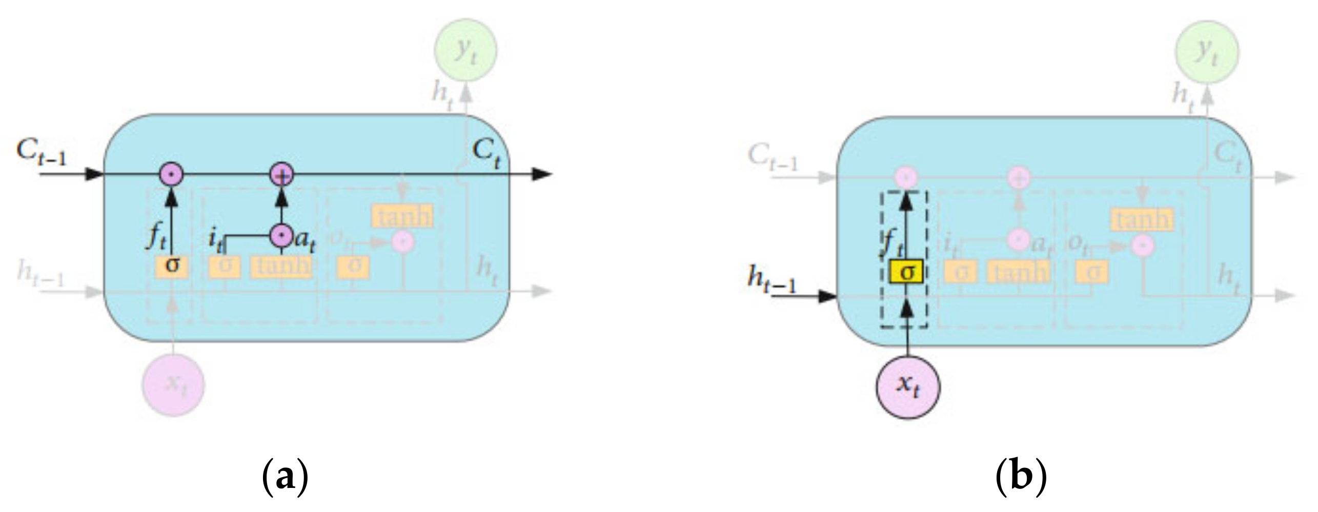
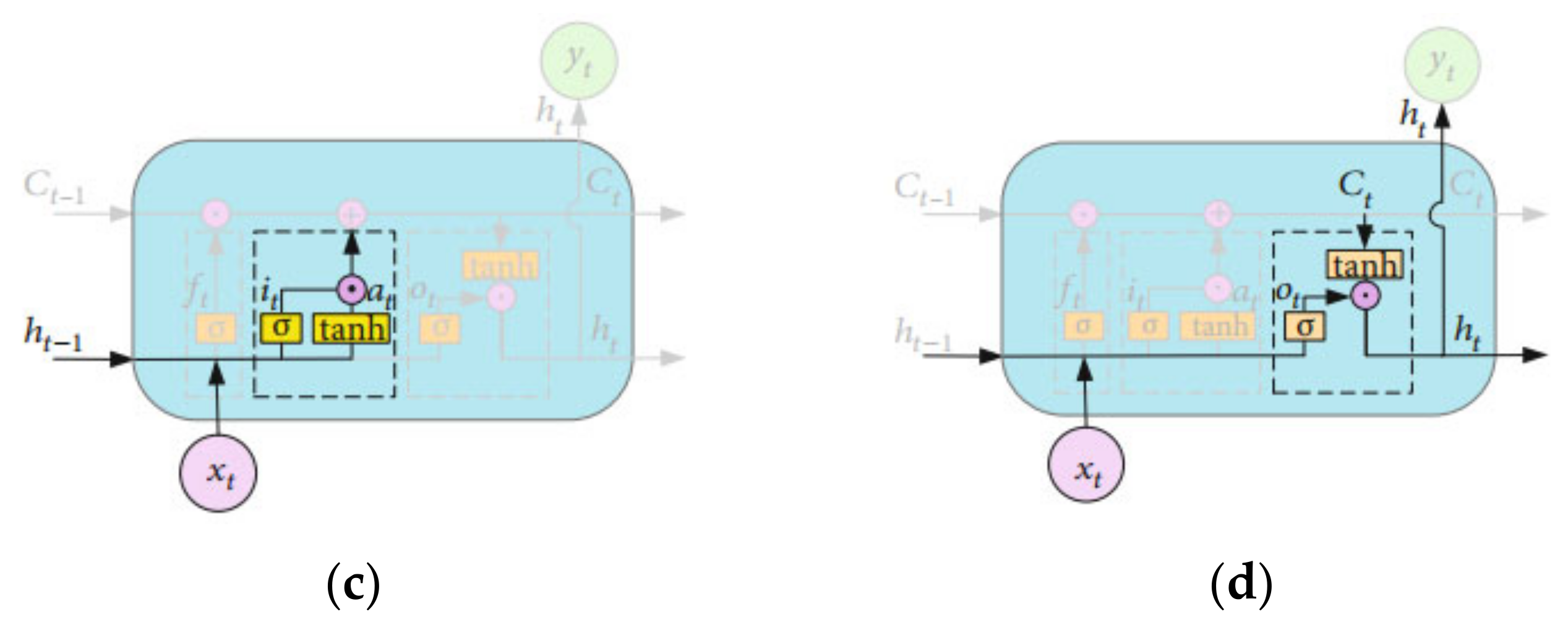
The core of the LSTM is the memory block, which includes three gate structures and a memory cell. Specifically, it consists of the cell state, forget gate, input gate, and output gate [47,48,49]. The LSTM gating mechanism is shown in Figure 2. Due to the presence of gate mechanisms in the LSTM network, the memory cell c can capture crucial information at a certain moment and retain this critical information for a certain period.
The specific computation process is as follows:
(1)
Initially, using the external state h t 1 from the previous time step and the current input x t , calculate the forget gate f t , input gate i t , and output gate o t ; then, compute the candidate value a t .
(2)
Combine f t and i t to determine whether to update the memory cell C t .
(3)
Combine o t to output the updated internal state information from the gate mechanism to the external state h t .

3.2. Sparrow Search Algorithm

The Sparrow Search Algorithm (SSA) is a swarm intelligence optimization algorithm proposed by Xue et al., in 2020, inspired by the foraging and predator evasion behavior of sparrows [50]. The SSA algorithm comprises three types of sparrows: explorers, joiners, and scouts. Explorers have higher fitness values, allowing them to prioritize food acquisition during the search process, guiding the overall movement of the sparrow flock. As a result, explorers can search for food in a broader area than joiners. The update function for explorers is as follows:
x i , j t + 1 = x i , j t exp i α T                                           R 2 < S T x i , j t + Q L                                                         R 2 > S T
where, t represents the current iteration, T is the maximum number of iterations, x i , j t is the value of the j dimension of the i th sparrow at iteration t , α is a random number in the range (0,1], R 2 R 2 0,1 , and S T S T 0,1 represent the early warning value and safety threshold, respectively; furthermore, Q is a random number following a normal distribution, and L is a 1 × d matrix with elements equal to 1.
When R 2 < S T , indicating that no predators are detected in the environment, explorers can search in a larger area. Conversely, if R 2 S T , signaling that some sparrows in the population have detected predators and issued an alert, all sparrows need to quickly fly to other safe locations for foraging.
During foraging, some joiners constantly monitor the explorers. Once they perceive that an explorer has found better food, they immediately leave their current position to compete for the food. If they succeed, they can immediately obtain the food found by the explorer. The update function for joiners is as follows:
x i , j t + 1 = x i , j t exp x w o r s t t x i , j t t 2 i < n 2 x P t + 1 + x i , j t x P t + 1 A + L o t h e r w i s e
where, x P is the optimal position occupied by the current explorer, x w o r s t represents the current globally worst position, and A is a 1 × d matrix with each element randomly assigned to 1 or −1, and A + = A T A A T 1 . When i > n/2, indicating that the i th joiner with lower fitness has not obtained food and is in a very hungry state, it needs to fly to another place for foraging to gain more energy.
Scouts typically constitute 10% to 20% of the sparrow flock, with random initial positions. The update function for scouts is as follows:
x i , j t + 1 = x best t + β . x i , j t x best t                                   f i > f g x P t + K . x i , j t x worst t f i f w + ε                             f i = f g
where, x b e s t is the best position in the sparrow population, β is a step-size control parameter following a normal distribution with mean 0 and variance 1, K 1,1 is a random number, f i is the fitness value of the current sparrow individual, f g and f w are the current global best and worst fitness values, ε is a constant to avoid division by zero, and K represents the direction of sparrow movement and is also a step-size control parameter.
When f i > f g , it indicates that the sparrow is on the edge of the population and is highly susceptible to predator attacks. When f i = f g , it means the sparrow in the middle of the population has realized the danger and needs to move closer to other sparrows to minimize the risk of predation.
SSA has the advantages of strong optimization ability and fast convergence. It demonstrates certain advantages in handling nonlinear, multivariate problems and can be used for optimizing parameters in LSTM models, thereby improving the accuracy of monitoring data predictions. In this study, the number of iterations, the number of nodes in two hidden layers, and the number of training samples selected in the model are chosen as optimization objectives for the SSA.

3.3. EMD-SSA-LSTM Prediction Model Calculation Process

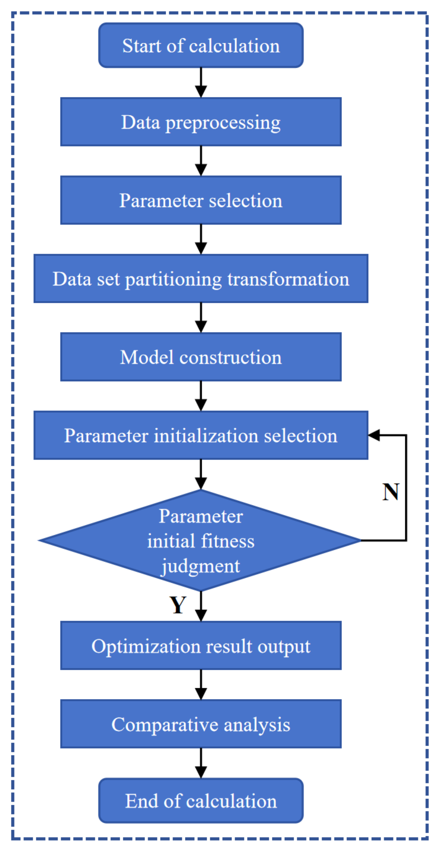
Based on the Long Short-Term Memory (LSTM) network and the Sparrow Search Algorithm (SSA) intelligent optimization, a multivariate time series prediction model for seepage flow in earth-rock dams is constructed. The calculation flow chart of the prediction model is shown in Figure 3. The specific process is as follows:
(1)
Data preprocessing: For the collected seepage flow monitoring data of the dam, the preprocessing method in Section 2.1 is used to handle outliers without compromising the integrity and trend of the original data.
(2)
Parameter selection: Taking dam seepage pressure as an example, along with the collected environmental factors, 15 influencing factors, including water pressure, temperature, and aging, are selected for factor parameter configuration. The mathematical model is shown in Equation (7).
(3)
Data set partitioning and transformation: The preprocessed data are transformed into supervised learning data using the series_to_supervised function to construct a 3-to-1 supervised learning data type, predicting the current day’s data using the data from the previous three days. A total of 16 years of monitoring data from 2004 to 2020 was collected, with the first 90% used as training data and the last 10% (approximately 2 years) used as prediction data, with normalization applied to the data using the MinMaxScaler function.
(4)
Model construction: For the prediction of dam seepage data, an LSTM neural network is built based on Tensorflow. To improve computational efficiency, GPU support is utilized, and a double-layer LSTM neural network is constructed.
(5)
Model initialization: The iteration count, the number of nodes in two hidden layers, and the training sample size in the LSTM neural network model are selected as optimization objectives. The SSA algorithm is initialized with the iteration count, population size, producer ratio, and initial parameter threshold, followed by the initialization calculation. See as Table 1.
(6)
Fitness calculation: The validation set mean squared error is used as the fitness function to find a set of hyperparameters that minimize the network’s error. Equations (8)–(10) are employed to update the positions of the sparrows in SSA, obtaining new fitness values for the sparrow population and saving the optimal individual and global optimal positions in the population.
(7)
Output optimization results: The particle values calculated by SSA optimization are used as the iteration count, the number of nodes in two hidden layers, and the training sample size for the LSTM neural network model.
(8)
Calculation and comparative analysis: For the predicted data, metrics such as Mean Squared Error (MSE), Root Mean Squared Error (RMSE), Mean Absolute Percentage Error (MAPE), Mean Absolute Error (MAE), and R-squared (R2) are used to evaluate the model accuracy. A comparative analysis is conducted with the prediction effects of GPU, Recurrent Neural Network (RNN), Backpropagation Neural Network (BPNN), and the commonly used multiple linear regression.

4. Study Area Introduction

The selected research object is the Siminghu Reservoir in Yuyao City, Zhejiang Province. Siminghu Reservoir is a large-scale reservoir primarily used for irrigation, with integrated functions such as flood control, water supply, and aquaculture. The total storage capacity is 1.2272 billion m3. Construction of the project began in 1958, and the dam was sealed in July 1959. Risk reinforcement was carried out from 2002 to 2004. The reservoir is designed to withstand floods with a return period of 100 years, and the verification is conducted for floods with a return period of 10,000 years. The normal water level of the reservoir is 16.28 m (elevation 85, the same below), corresponding to a storage capacity of 0.7946 billion m3. The dead water level is 6.78 m, and the flood limit water level is 15.28 m. The design flood level is 17.88 m, corresponding to a storage capacity of 0.9774 billion m3. The verified flood level is 19.85 m, corresponding to a storage capacity of 1.2272 billion m3. The Siminghu Reservoir’s reservoir hub project consists of a river-blocking dam, flood discharge gate, self-destroying spillway, water conveyance tunnel, discharge and supply water tunnel, and a power station.
The river-blocking dam is an earth-rock dam with a maximum height of 16.85 m. It is reinforced with a combination of clay slanting walls and composite geomembranes for seepage prevention. The dam crest elevation is 21.13 m, with a length of 600 m and a width of 5.5 m. There is a wave-prevention wall with a height of 1.2 m. The upstream slope ratio is 1:3.7, protected by concrete prefabricated block revetment, while the downstream slope ratios are 1:2.2 and 1:2.5 from top to bottom, protected by granite cobblestone revetment.
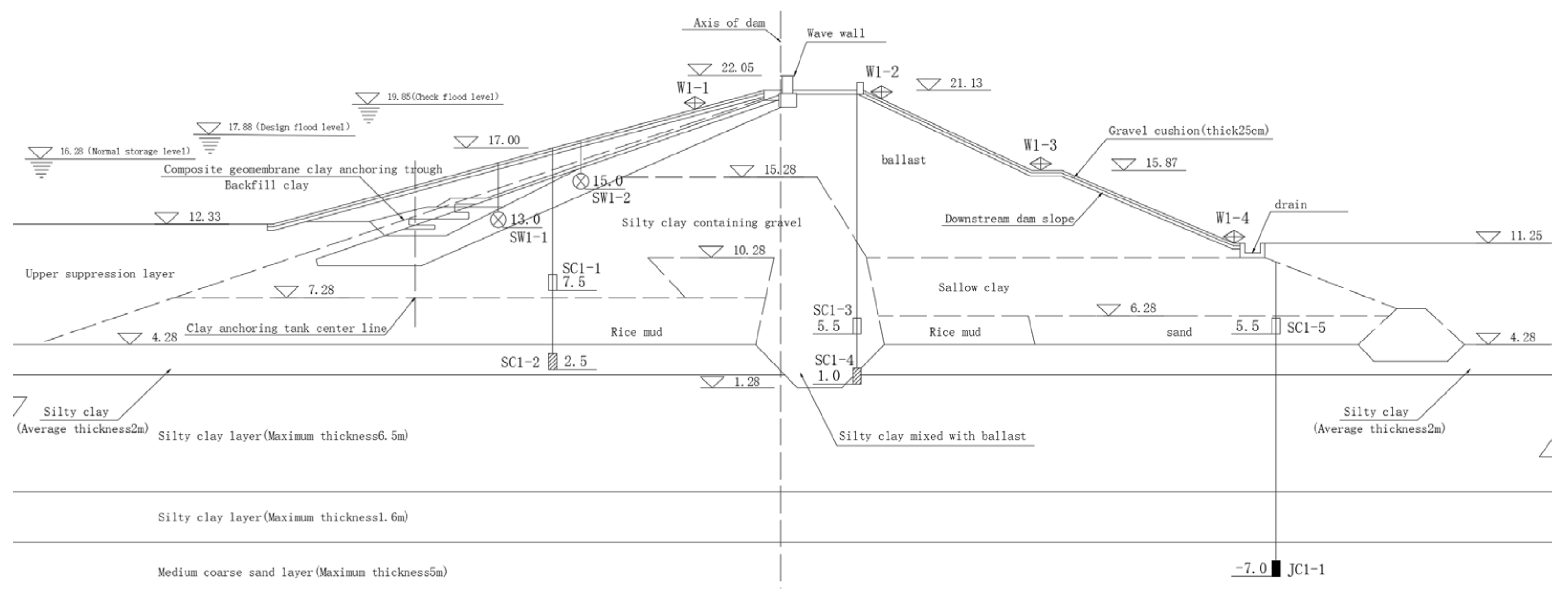
For the monitoring points of seepage pressure in the Siminghu Reservoir dam, points were selected based on the overall integrity of monitoring instrument performance, the accuracy of instruments meeting specification requirements, and the physical significance, continuity, and consistency of monitoring data. The arrangement of seepage monitoring instruments is shown in Figure 4. The selected monitoring points are listed in Table 2.

5. Results and Discussion

5.1. EMD-SSA-LSTM Prediction Model Calculation Process

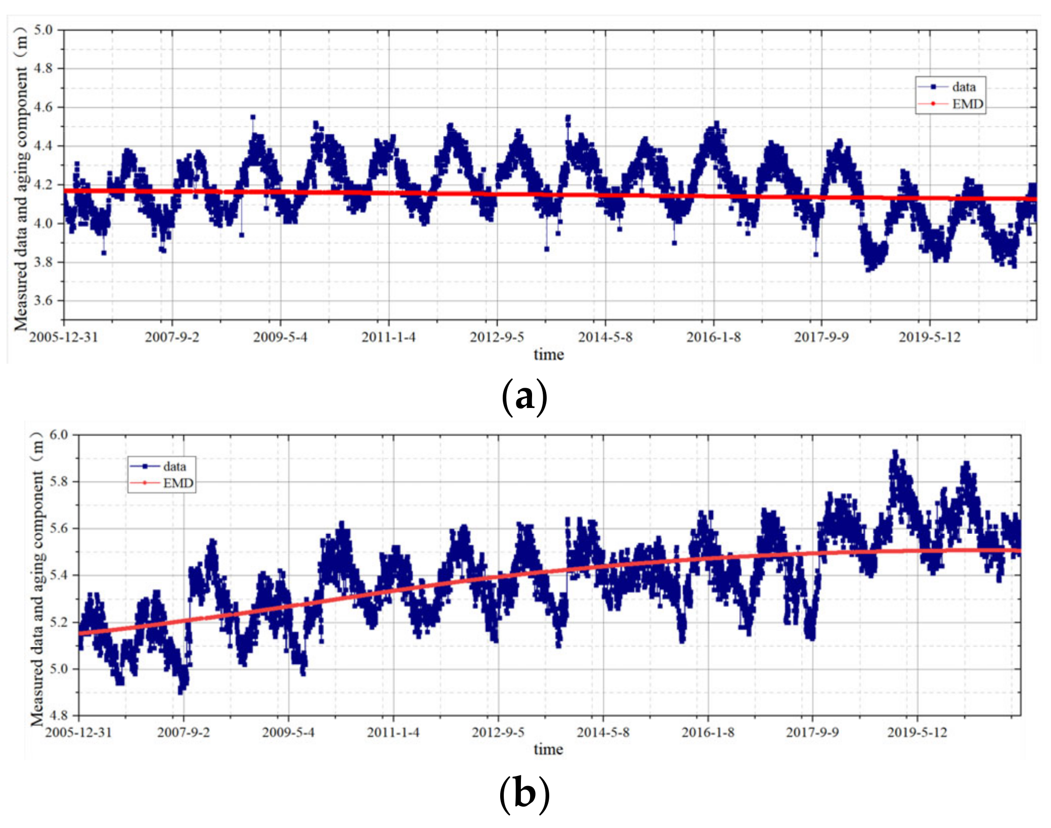
For the four monitoring points in Table 2, the seepage pressure monitoring data from 1 January 2006 to 31 December 2020 was selected as the analysis period for predicting the safety status of the dam. The data from 31 December 2018 to 31 December 2020 was chosen as the prediction period. From the time series monitoring data, a slight time-dependent trend is still evident. To enhance the reliability of the results in the prediction analysis of the dam’s safety status, Empirical Mode Decomposition (EMD) was employed to separate the time-dependent components from the seepage pressure monitoring data of the earth-rock dam. The results of separating the trend components for each monitoring point are shown in the following Figure 5.

5.2. Parameter Optimization of Multivariate Time Prediction Model

The adjustment of hyperparameters in a neural network includes parameters related to network design and those related to the training process. Network design related parameters encompass the number of layers, the types of layers, their sequence, the configuration of neurons in the hidden layers, the choice of loss function, optimizer selection, and regularization parameters. On the other hand, training process related parameters involve network weights, initialization schemes, learning rate, the number of epochs, and the batch size.
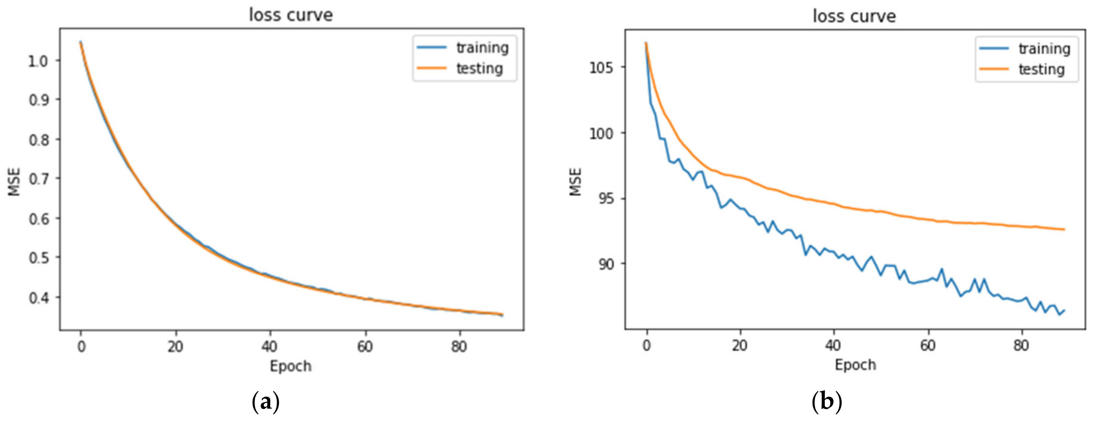
For a neural network model, parameter tuning is necessary when the Loss curve fits perfectly, underfits, or overfits, aiming to achieve optimal predictive performance. The results of neural network training are shown in Figure 6.
Adjustments can be made in several aspects, including the number of neurons in the hidden layers, the number of epochs, the batch size, the choice of loss function, and the selection of the optimizer. The SSA (Sparrow Search Algorithm) is employed for tuning the number of neurons in the hidden layers, the number of epochs, and the batch size. This section focuses on optimizing the selection of the loss function and the optimizer.
  • Optimizer
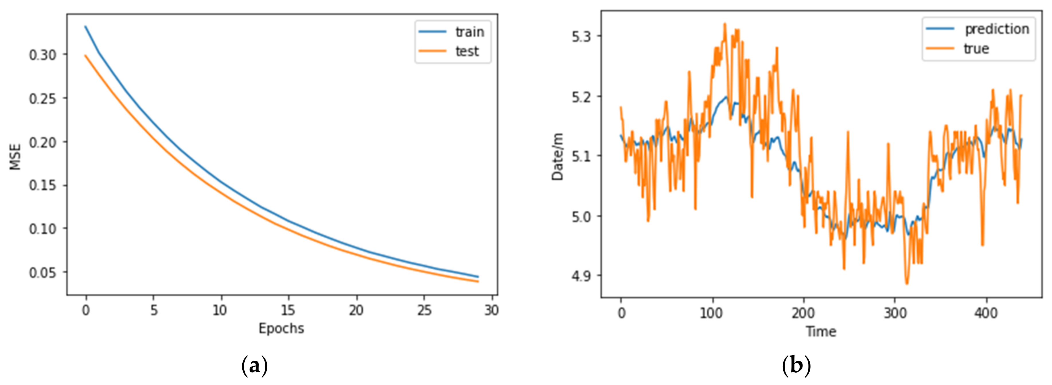
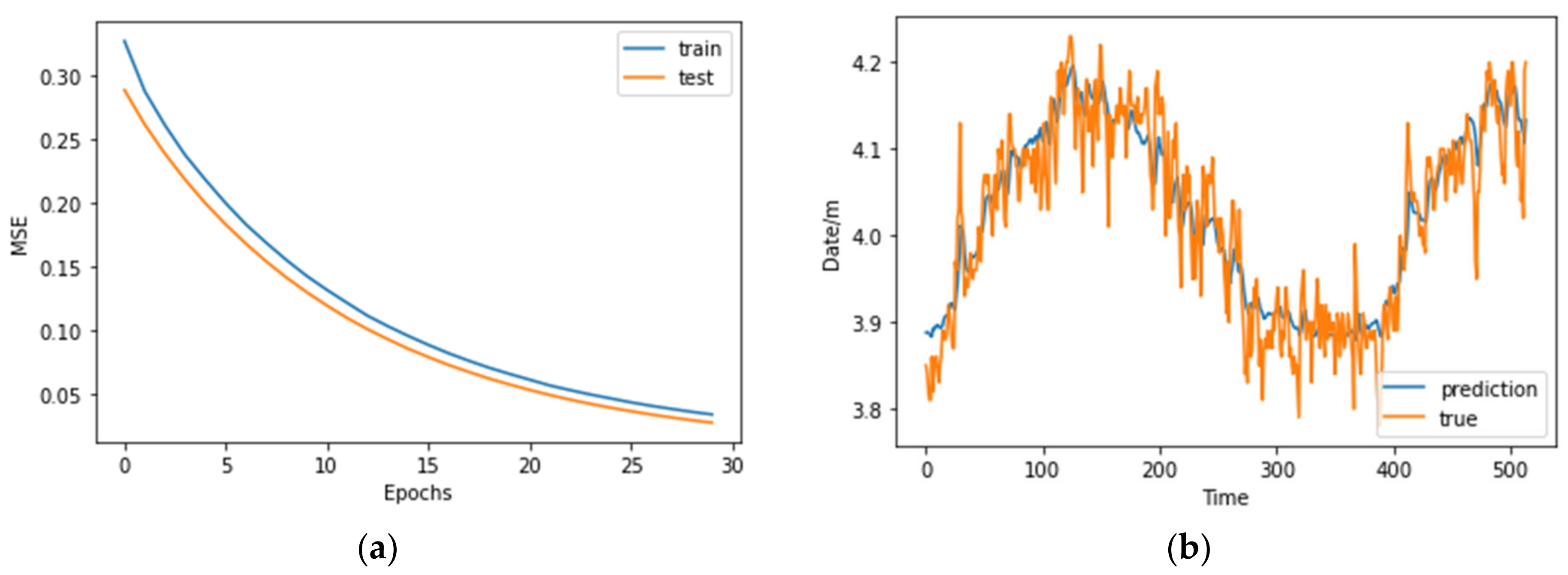
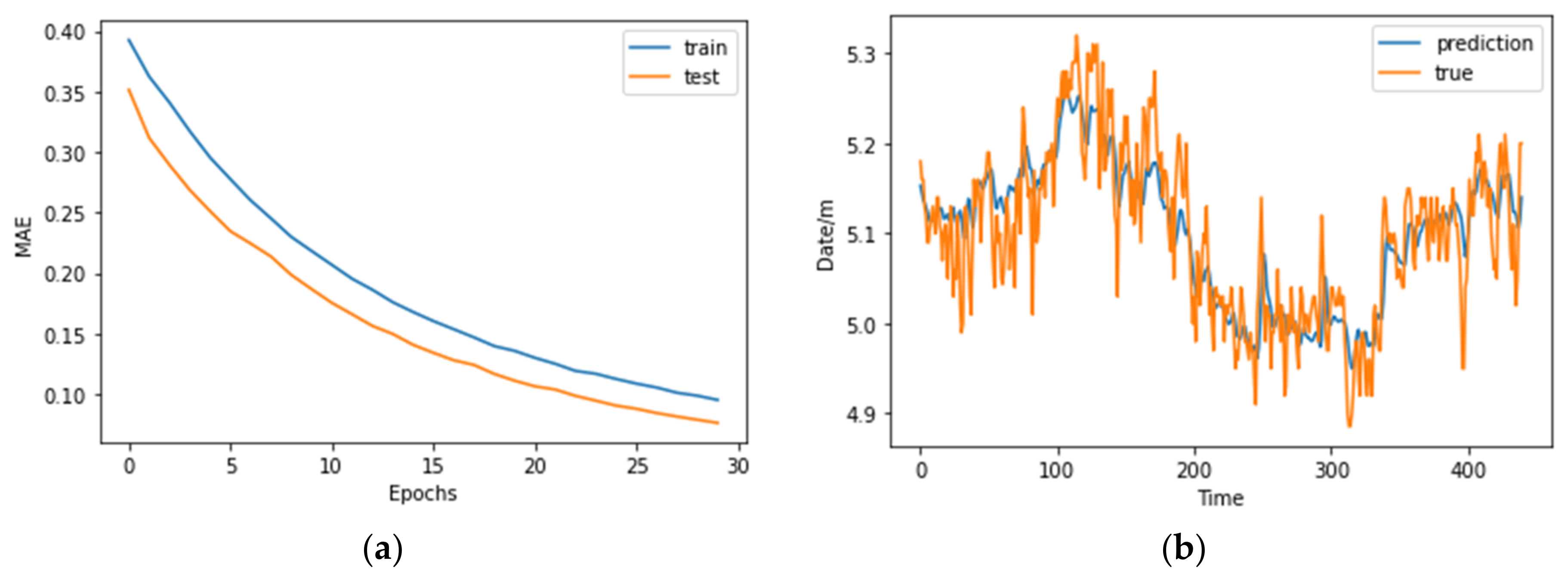
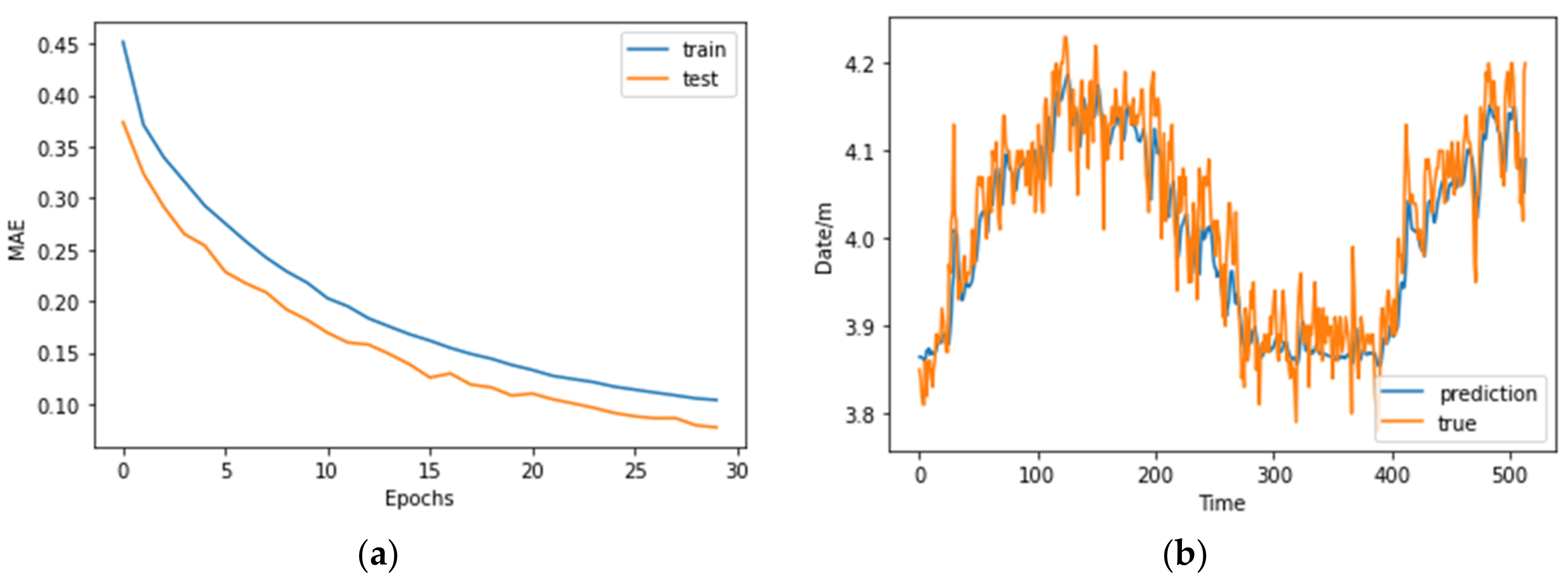
The optimizer guides the loss function to update the parameters in the correct direction with an appropriate magnitude. The updated parameters continuously approach the global optimum. Tuning was performed on the preprocessed JC1−2 and SC2−6 monitoring points. Under the Mean Squared Error (MSE) loss function, various optimization functions were compared and analyzed, and the specific results are shown in Table 3. The final choice was the Adagrad algorithm, which demonstrated the optimal optimization effect and results. The optimization process and results of the Adagrad optimizer are shown in Figure 7 and Figure 8. The formula for the Adagrad algorithm is as follows:
w t + 1 = w t a m t / V t = w t a m t / t = 1 t g t 2
where, a is the learning rate and g t is the gradient of the current parameter.
2.
Loss Function
The loss function is used to evaluate the discrepancy between the model’s predicted values f x and the actual values y . By minimizing the loss function, the goal is to make the predicted values f x as close as possible to the actual values y . Given that the optimizer is Adagrad, different loss functions were compared. Common choices for regression problems include Mean Squared Error (MSE), Mean Absolute Error (MAE), Squared Hinge, LogCosh, etc.
The Mean Absolute Error (MAE) was selected as the loss function due to its optimal performance. MAE is insensitive to outliers and exhibits inclusivity, meaning the model’s penalty strength and weight are the same for all data points. The MAE loss function optimization process and results are shown in Figure 9 and Figure 10. The optimization effects of different loss functions are shown in Table 4. Therefore, MAE has better robustness for volatile data. The definition expression for Mean Absolute Error (MAE) is as follows:
M A E = i 1 n y i x i n
3.
Comparative analysis of prediction accuracy
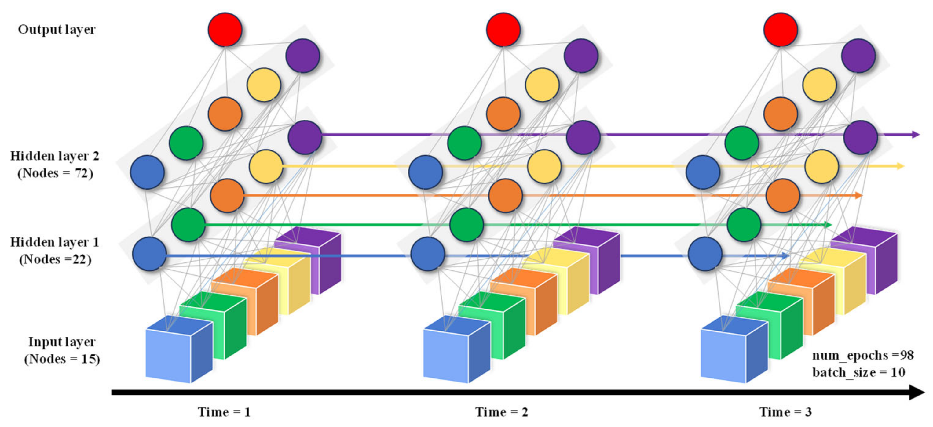
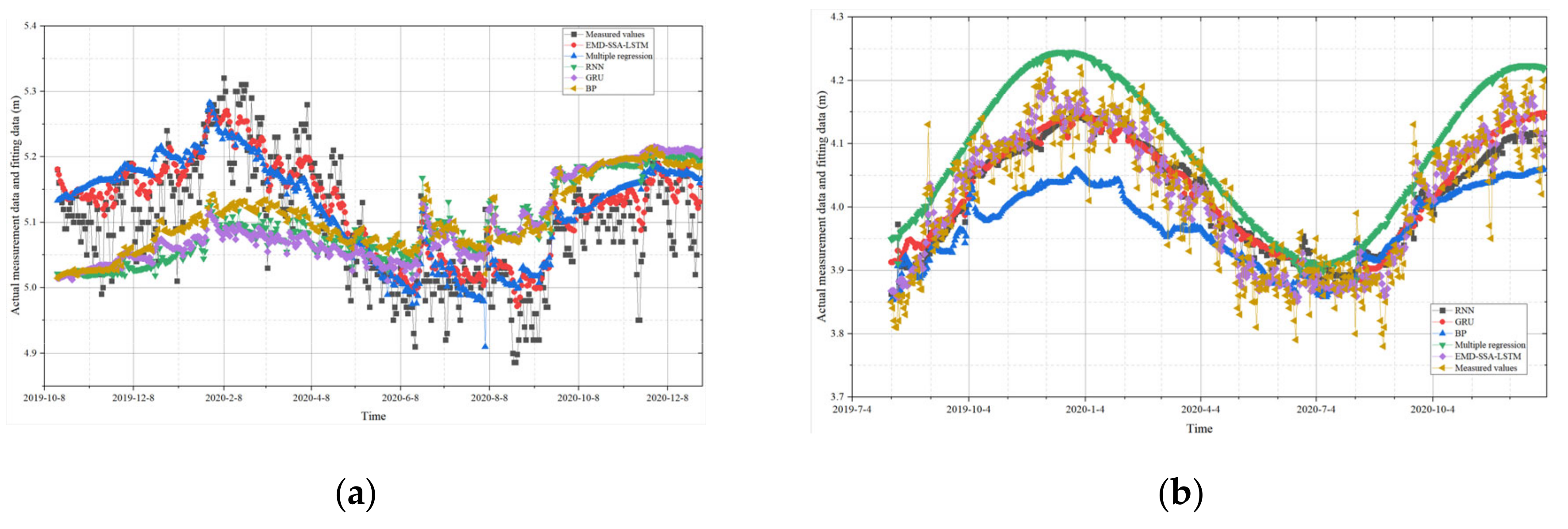
The predictive models established using EMD-SSA-LSTM, RNN, GRU, BP neural network, and multivariate linear regression for the prediction of seepage pressure in the dam were compared. The constructed LSTM structure of JC2−1, for example, is shown in Figure 11. The measured values and predicted values for the monitoring points JC1-2, SC2-6, SW3-1, and JC4-2 under different models are shown in Figure 12. The process lines of each model and the fitting lines exhibit similar patterns, consistent trends, and good overall agreement. Notably, the EMD-SSA-LSTM neural network provides better fitting results, with a more pronounced trend. The evaluation indicators in Table 5, Table 6, Table 7 and Table 8 indicate that the EMD-SSA-LSTM neural network model outperforms other algorithms in various aspects.
According to Figure 13, the fluctuation of error values in the EMD-SSA-LSTM results is smaller, indicating that the model achieves high predictive accuracy after training and meets the requirements for prediction.

6. Conclusions

(1) Compared to traditional statistical regression models, EMD has the advantage of convenient computation and does not require the pre-assumption of time-effect functions.
(2) A multivariate time series prediction model based on the sparrow optimization algorithm and the long short-term memory neural network (LSTM) is established. The influence of different neural network parameter selections on model gradient descent and prediction results is analyzed. “Adagrad” and “MAE” are selected as the optimizer and loss function for the prediction model, resulting in a well-fitted Loss curve.
(3) A comparative analysis is conducted on the prediction accuracy of the SSA-LSTM model compared to BP, RNN, GRU, and other neural networks, as well as multivariate linear regression methods. The prediction model’s parameters outperform other methods, indicating high predictive accuracy and suitability for forecasting future trends in monitoring points.

Author Contributions

Conceptualization, X.Y.; methodology, Y.X.; software, Y.W.; validation, G.S.; formal analysis, Y.W.; investigation, X.Y.; resources, Y.X.; data curation, Y.W.; writing—original draft preparation, Y.W.; writing—review and editing, X.Y.; visualization, G.S.; supervision, Y.X.; project administration, X.Y. All authors have read and agreed to the published version of the manuscript.

Funding

This research was supported by the National Key R&D Program of China (2022YFC3005405), the National Natural Science Foundation of China (Grant No. U23B20150 and 52309159), the Major science and technology project of the Ministry of Water Resources of China (SK-2022096), and the Science and Technology Project of Yunnan Province (202203AA080009).

Data Availability Statement

Data are contained within the article.

Conflicts of Interest

The authors declare no conflicts of interest.

References

  1. Prakash, G.; Dugalam, R.; Barbosh, M.; Sadhu, A. Recent Advancement of Concrete Dam Health Monitoring Technology: A Systematic Literature Review. Structures 2022, 44, 766–784. [Google Scholar] [CrossRef]
  2. Ma, C.; Xu, X.; Yang, J.; Cheng, L. Safety Monitoring and Management of Reservoir and Dams. Water 2023, 15, 1078. [Google Scholar] [CrossRef]
  3. Garsole, P.A.; Bokil, S.; Kumar, V.; Pandey, A.; Topare, N.S. A Review of Artificial Intelligence Methods for Predicting Gravity Dam Seepage, Challenges and Way-Out. AQUA Water Infrastruct. Ecosyst. Soc. 2023, 72, 1228–1248. [Google Scholar] [CrossRef]
  4. Salazar, F.; Morán, R.A.; Angel, M.; Oñate, E. Data-Based Models for the Prediction of Dam Behaviour: A Review and Some Methodological Considerations. Arch. Comput. Methods Eng. 2017, 24, 1–21. [Google Scholar] [CrossRef]
  5. Zhu, Y.; Niu, X.; Gu, C.; Yang, D.; Sun, Q.; Fernández-Rodríguez, E. Using the DEMATEL-VIKOR Method in Dam Failure Path Identification. Int. J. Environ. Res. Public Health 2020, 17, 1480. [Google Scholar] [CrossRef] [PubMed]
  6. Sivasuriyan, A.; Vijayan, D.S.; Munusami, R.; Devarajan, P. Health Assessment of Dams under Various Environmental Conditions Using Structural Health Monitoring Techniques: A State-of-Art Review. Environ. Sci. Pollut. Res. 2021, 29, 86180–86191. [Google Scholar] [CrossRef] [PubMed]
  7. Adamo, N.; Al-Ansari, N.; Sissakian, V.; Laue, J.; Knutsson, S. Dam Safety: Use of Instrumentation in Dams. J. Earth Sci. Geotech. Eng. 2020, 11, 145–202. [Google Scholar] [CrossRef]
  8. Li, B.; Yang, J.; Hu, D. Dam Monitoring Data Analysis Methods: A Literature Review. Struct. Control Health Monit. 2019, 27, e2501. [Google Scholar] [CrossRef]
  9. Chen, S.; Gu, C.; Lin, C.; Zhang, K.; Zhu, Y. Multi-Kernel Optimized Relevance Vector Machine for Probabilistic Prediction of Concrete Dam Displacement. Eng. Comput. 2020, 37, 1943–1959. [Google Scholar] [CrossRef]
  10. Yang, X.; Xiang, Y.; Shen, G.; Sun, M. A Combination Model for Displacement Interval Prediction of Concrete Dams Based on Residual Estimation. Sustainability 2022, 14, 16025. [Google Scholar] [CrossRef]
  11. Zhang, K.; Gu, C.; Zhu, Y.; Chen, S.; Dai, B.; Li, Y.; Shu, X. A Novel Seepage Behavior Prediction and Lag Process Identification Method for Concrete Dams Using HGWO-XGBoost Model. IEEE Access 2021, 9, 23311–23325. [Google Scholar] [CrossRef]
  12. Yang, D.; Gu, C.; Zhu, Y.; Dai, B.; Zhang, K.; Zhang, Z.; Li, B. A Concrete Dam Deformation Prediction Method Based on LSTM with Attention Mechanism. IEEE Access 2020, 8, 185177–185186. [Google Scholar] [CrossRef]
  13. Gu, C.; Fu, X.; Shao, C.; Shi, Z.; Su, H. Application of Spatiotemporal Hybrid Model of Deformation in Safety Monitoring of High Arch Dams: A Case Study. Int. J. Environ. Res. Public Health 2020, 17, 319. [Google Scholar] [CrossRef] [PubMed]
  14. Zhu, Y.; Xie, M.; Zhang, K.; Li, Z. A Dam Deformation Residual Correction Method for High Arch Dams Using Phase Space Reconstruction and an Optimized Long Short-Term Memory Network. Mathematics 2023, 11, 2010. [Google Scholar] [CrossRef]
  15. Zhang, F.; Lu, X.; Li, Y.; Gao, Z.; Zhang, H.; Huang, H. A Self-Matching Model for Online Anomaly Recognition of Safety Monitoring Data in Dams. Struct. Health Monit. 2022, 22, 746–773. [Google Scholar] [CrossRef]
  16. Mohammadi, M.; Al-Fuqaha, A.; Sorour, S.; Guizani, M. Deep Learning for IoT Big Data and Streaming Analytics: A Survey. IEEE Commun. Surv. Tutor. 2018, 20, 2923–2960. [Google Scholar] [CrossRef]
  17. Li, M.; Shen, Y.; Ren, Q.; Li, H. A New Distributed Time Series Evolution Prediction Model for Dam Deformation Based on Constituent Elements. Adv. Eng. Inform. 2019, 39, 41–52. [Google Scholar] [CrossRef]
  18. Ribeiro, L.S.; Wilhelm, V.E.; de Jairo Marlon Corrêa, F.; Santos, A. A Comparative Analysis of Long-Term Concrete Deformation Models of a Buttress Dam. Eng. Struct. 2019, 193, 301–307. [Google Scholar] [CrossRef]
  19. Chen, B.; Hu, T.; Huang, Z.; Fang, C. A Spatio-Temporal Clustering and Diagnosis Method for Concrete Arch Dams Using Deformation Monitoring Data. Struct. Health Monit. 2018, 18, 1355–1371. [Google Scholar] [CrossRef]
  20. Mata, J. Interpretation of Concrete Dam Behaviour with Artificial Neural Network and Multiple Linear Regression Models. Eng. Struct. 2011, 33, 903–910. [Google Scholar] [CrossRef]
  21. Sharma, M.J.; Yu, S.J. Stepwise Regression Data Envelopment Analysis for Variable Reduction. Appl. Math. Comput. 2015, 253, 126–134. [Google Scholar] [CrossRef]
  22. Yu, H.; Wu, Z.; Bao, T.; Zhang, L. Multivariate Analysis in Dam Monitoring Data with PCA. Sci. China Technol. Sci. 2010, 53, 1088–1097. [Google Scholar] [CrossRef]
  23. Hu, W.L.; Deng, N.W.; Liu, Q.S. Optimization Study of Stepwise Regression and Partial Least Squares Regression Models for Dam Security Monitoring. Appl. Mech. Mater. 2014, 578–579, 1101–1107. [Google Scholar] [CrossRef]
  24. Tatin, M.; Briffaut, M.; Dufour, F.; Simon, A.; Fabre, J.-P. Statistical Modelling of Thermal Displacements for Concrete Dams: Influence of Water Temperature Profile and Dam Thickness Profile. Eng. Struct. 2018, 165, 63–75. [Google Scholar] [CrossRef]
  25. Sevieri, G.; De Falco, A. Dynamic Structural Health Monitoring for Concrete Gravity Dams Based on the Bayesian Inference. J. Civ. Struct. Health Monit. 2020, 10, 235–250. [Google Scholar] [CrossRef]
  26. Wang, S.; Xu, C.; Liu, Y.; Wu, B. A Spatial Association-Coupled Double Objective Support Vector Machine Prediction Model for Diagnosing the Deformation Behaviour of High Arch Dams. Struct. Health Monit. 2021, 21, 945–964. [Google Scholar] [CrossRef]
  27. Li, Z.; Yin, C.; Chen, R.; Wu, Z.; Chen, J.; Lu, X. A novel deformation monitoring model for high arch dams using impulse response-based equivalent temperature and machine learning-aided separate modeling. Expert Syst. Appl. 2024, 238, 122328. [Google Scholar] [CrossRef]
  28. Nguyen, L.H.; Goulet, J. Real-Time Anomaly Detection with Bayesian Dynamic Linear Models. Struct. Control Health Monit. 2019, 26, e2404. [Google Scholar] [CrossRef]
  29. Zhang, S.; Zheng, D.; Liu, Y. Deformation Prediction System of Concrete Dam Based on IVM-SCSO-RF. Water 2022, 14, 3739. [Google Scholar] [CrossRef]
  30. Lei, W.; Wang, J. Dynamic Stacking Ensemble Monitoring Model of Dam Displacement Based on the Feature Selection with PCA-RF. J. Civ. Struct. Health Monit. 2022, 12, 557578. [Google Scholar] [CrossRef]
  31. Su, H.; Wen, Z.; Chen, Z.; Tian, S. Dam Safety Prediction Model Considering Chaotic Characteristics in Prototype Monitoring Data Series. Struct. Health Monit. 2016, 15, 639–649. [Google Scholar] [CrossRef]
  32. Yavaşoğlu, H.H.; Kalkan, Y.; Tiryakioğlu, İ.; Yigit, C.O.; Özbey, V.; Alkan, M.N.; Bilgi, S.; Alkan, R.M. Monitoring the Deformation and Strain Analysis on the Ataturk Dam, Turkey. Geomat. Nat. Hazards Risk 2017, 9, 94–107. [Google Scholar] [CrossRef]
  33. Zhu, Y.; Zhang, Z.; Gu, C.; Li, Y.; Zhang, K.; Xie, M. A Coupled Model for Dam Foundation Seepage Behavior Monitoring and Forecasting Based on Variational Mode Decomposition and Improved Temporal Convolutional Network. Struct. Control. Health Monit. 2023, 2023, 3879096. [Google Scholar] [CrossRef]
  34. Hariri-Ardebili, M.A.; Mahdavi, G.; Nuss, L.K.; Lall, U. The Role of Artificial Intelligence and Digital Technologies in Dam Engineering: Narrative Review and Outlook. Eng. Appl. Artif. Intell. 2023, 126, 106813. [Google Scholar] [CrossRef]
  35. Chen, W.; Wang, X.; Tong, D.; Cai, Z.; Zhu, Y.; Liu, C. Dynamic Early-Warning Model of Dam Deformation Based on Deep Learning and Fusion of Spatiotemporal Features. Knowl. Based Syst. 2021, 233, 107537. [Google Scholar] [CrossRef]
  36. El Bilali, A.; Moukhliss, M.; Taleb, A.; Nafii, A.; Alabjah, B.; Brouziyne, Y.; Mazigh, N.; Teznine, K.; Mhamed, M. Predicting Daily Pore Water Pressure in Embankment Dam: Empowering Machine Learning-Based Modeling. Environ. Sci. Pollut. Res. 2022, 29, 47382–47398. [Google Scholar] [CrossRef]
  37. Johari, A.; Talebi, A.; Heydari, A. Prediction of Discharge Flow Rate beneath Sheet Piles Using Gene Expression Programming Based on Scaled Boundary Finite Element Modelling Database. Sci. Iran. 2020, 28, 645–655. [Google Scholar] [CrossRef]
  38. Zhang, C.; Fu, S.; Ou, B.; Liu, Z.; Hu, M. Prediction of Dam Deformation Using SSA-LSTM Model Based on Empirical Mode Decomposition Method and Wavelet Threshold Noise Reduction. Water 2022, 14, 3380. [Google Scholar] [CrossRef]
  39. Wei, B.; Chen, L.; Li, H.; Yuan, D.; Wang, G. Optimized Prediction Model for Concrete Dam Displacement Based on Signal Residual Amendment. Appl. Math. Model. 2020, 78, 20–36. [Google Scholar] [CrossRef]
  40. Yuan, D.; Wei, B.; Xie, B.; Zhong, Z. Modified Dam Deformation Monitoring Model Considering Periodic Component Contained in Residual Sequence. Struct. Control Health Monit. 2020, 27, e2633. [Google Scholar] [CrossRef]
  41. Li, H.; Li, Z.; Mo, W. A Time Varying Filter Approach for Empirical Mode Decomposition. Signal Process. 2017, 138, 146–158. [Google Scholar] [CrossRef]
  42. Chen, S.; Cao, S.; Sun, Y.; Lin, Y.; Gao, J. Seismic Time-Frequency Analysis via Time-Varying Filtering Based Empirical Mode Decomposition Method. J. Appl. Geophys. 2022, 204, 104731. [Google Scholar] [CrossRef]
  43. Stallone, A.; Cicone, A.; Materassi, M. New Insights and Best Practices for the Successful Use of Empirical Mode Decomposition, Iterative Filtering and Derived Algorithms. Sci. Rep. 2020, 10, 15161. [Google Scholar] [CrossRef] [PubMed]
  44. Stefenon, S.F.; Ribeiro, M.H.D.M.; Nied, A.; Yow, K.C.; Mariani, V.C.; dos Santos Coelho, L.; Seman, L.O. Time Series Forecasting Using Ensemble Learning Methods for Emergency Prevention in Hydroelectric Power Plants with Dam. Electr. Power Syst. Res. 2022, 202, 107584. [Google Scholar] [CrossRef]
  45. Xu, S.; Li, W.; Zhu, Y.; Xu, A. A Novel Hybrid Model for Six Main Pollutant Concentrations Forecasting Based on Improved LSTM Neural Networks. Sci. Rep. 2022, 1, 144342. [Google Scholar] [CrossRef]
  46. Reddybattula, K.D.; Nelapudi, L.S.; Moses, M.; Devanaboyina, V.R.; Ali, M.A.; Jamjareegulgarn, P.; Panda, S.K. Ionospheric TEC Forecasting over an Indian Low Latitude Location Using Long Short-Term Memory (LSTM) Deep Learning Network. Universe 2022, 8, 562. [Google Scholar] [CrossRef]
  47. Yu, Y.; Si, X.; Hu, C.; Zhang, J. A Review of Recurrent Neural Networks: LSTM Cells and Network Architectures. Neural Comput. 2019, 31, 1235–1270. [Google Scholar] [CrossRef]
  48. Wen, S.; Wei, H.; Yang, Y.; Guo, Z.; Zeng, Z.; Huang, T.; Chen, Y. Memristive LSTM Network for Sentiment Analysis. IEEE Trans. Syst. Man Cybern. Syst. 2019, 51, 1794–1804. [Google Scholar] [CrossRef]
  49. Vankadara, R.K.; Mosses, M.; Siddiqui, M.I.H.; Ansari, K.; Panda, S.K. Ionospheric Total Electron Content Forecasting at a Low-Latitude Indian Location Using a Bi-Long Short-Term Memory Deep Learning Approach. IEEE Trans. Plasma Sci. 2023, 51, 3373–3383. [Google Scholar] [CrossRef]
  50. Liu, R.; Mo, Y. Performance of a Novel Enhanced Sparrow Search Algorithm for Engineering Design Process: Coverage Optimization in Wireless Sensor Network. Processes 2022, 10, 1691. [Google Scholar] [CrossRef]
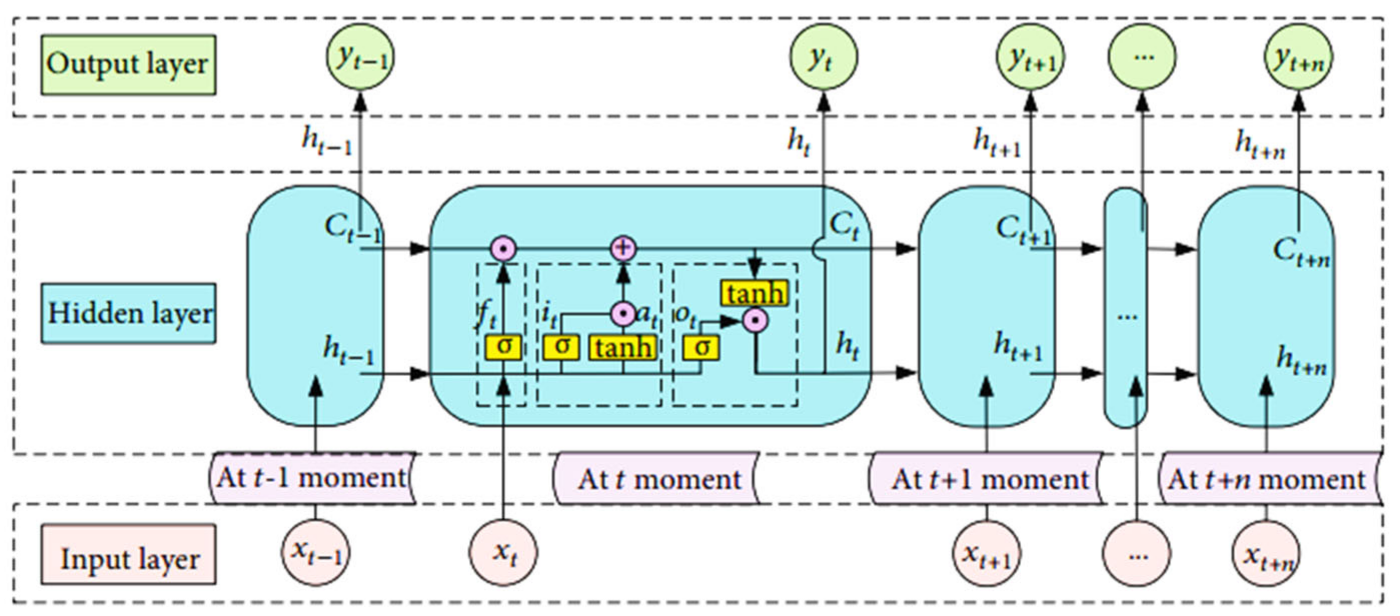
Figure 1. Cyclic unit structure of the LSTM network.
Water 16 00395 g001
Figure 2. LSTM gating mechanisms: (a) cell state; (b) forget gate; (c) input gate; (d) output gate.
Water 16 00395 g002aWater 16 00395 g002b
Figure 3. Flow chart of prediction model calculation.
Water 16 00395 g003
Figure 4. 0 + 105.00 m section seepage monitoring instrument layout.
Water 16 00395 g004
Figure 5. Measured data and aging component: (a) Monitoring point SC2-6; (b) Monitoring point JC4-2; (c) Monitoring point SW3-1; (d) Monitoring point JC1-2.
Water 16 00395 g005aWater 16 00395 g005b
Figure 6. Neural network training results: (a) Exact fit; (b) Underfitting.
Water 16 00395 g006
Figure 7. Adagrad optimizer optimization process and results (Monitoring point JC1−2): (a) Optimization procedure; (b) Result.
Water 16 00395 g007
Figure 8. Adagrad optimizer optimization process and results (Monitoring point SC2−6): (a) Optimization procedure; (b) Result.
Water 16 00395 g008
Figure 9. MAE loss function optimization process and results (Monitoring point JC1−2): (a) Optimization procedure; (b) Result.
Water 16 00395 g009
Figure 10. MAE loss function optimization process and results (Monitoring point SC2-6): (a) Optimization procedure; (b) Result.
Water 16 00395 g010
Figure 11. Diagram of the constructed LSTM structure (using JC2-1 as an example).
Water 16 00395 g011
Figure 12. Comparison of results of different prediction models: (a) Monitoring point JC1-2; (b) Monitoring point SC2-6; (c) Monitoring point SW3-1; (d) Monitoring point JC4-2.
Water 16 00395 g012aWater 16 00395 g012b
Figure 13. Comparison of results of different residual models: (a) Monitoring point JC1-2; (b) Monitoring point SC2-6; (c) Monitoring point SW3-1; (d) Monitoring point JC4-2.
Water 16 00395 g013
Table 1. SSA parameter selection.
Name of ParameterValue
Iterations10
Sparrow population20
Optimization dimension4
Finder alert threshold0.8
Finder ratio20%
Scout ratio20%
Data rangeIterations[10–100]
Number of nodes in the first hidden layer[1–100]
Number of nodes in the second hidden layer[1–100]
Number of samples selected for training[10–100]
Table 2. Seepage pressure monitoring point selection table of the Siminghu reservoir dam.
Hole NumberDam Axis Distance (m)Station Number
Under the geomembrane−18.50SW3-1
U-3+33.00JC4-2
U-4+100.00JC1-2, SC2-6
Table 3. Optimization effect of different deep learning optimizers (Monitoring point JC1−2).
Optimizer TypeMAPERMSEMAEMSER2
Adagrad0.00870.05690.04480.00320.6380
Adadelta0.02330.14050.11950.0197−1.2067
Adam0.03930.22280.20180.0496−4.5486
Adamax0.01000.06500.05100.00420.5270
Ftrl0.05420.29350.27790.0862−8.6334
Nadam0.01820.10820.09360.0117−0.3097
RMSprop0.01820.11240.09380.0126−0.4125
SGD0.00940.05990.04820.00350.5976
Table 4. Optimization effect of different loss functions (Monitoring point JC1-2).
Optimizer TypeMAPERMSEMAEMSER2
MSE0.00870.05690.04480.00320.6380
MAE0.00830.05280.04260.00270.6884
MAPE0.12440.65450.63600.4284−46.9011
MSLE0.00940.06110.04840.00370.5815
squared_hinge1.08735.55815.543730.8931−3452.79
categorical_hinge0.51522.65772.63087.0637−788.71
LogCosh0.01160.07310.05970.40240.0053
Table 5. Optimization effect of different loss functions (Monitoring point JC1-2).
Evaluation IndexEMD-SSA-LSTMRNNGRUBP Neural NetworkMultiple Linear Regression
MSE0.00260.01070.01060.00860.0038
RMSE0.05190.10350.10300.10520.0616
MAE0.04070.08840.08930.08540.0485
R20.6759−0.2892−0.2775−0.03560.6068
Table 6. Optimization effect of different loss functions (Monitoring point SC2-6).
Evaluation IndexEMD-SSA-LSTMRNNGRUBP Neural NetworkMultiple Linear Regression
MSE0.00160.00270.00260.00660.0071
RMSE0.04010.05160.05130.13520.0842
MAE0.03140.04100.04050.11290.0711
R20.86740.78030.78330.45040.8067
Table 7. Optimization effect of different loss functions (Monitoring point SW3-1).
Evaluation IndexEMD-SSA-LSTMRNNGRUBP Neural NetworkMultiple Linear Regression
MSE0.01560.00700.00700.03660.0113
RMSE0.03950.08380.08360.25840.1061
MAE0.03400.06260.06290.21200.0819
R20.91990.64040.6417−0.87650.7878
Table 8. Optimization effect of different loss functions (Monitoring point JC4−2).
Evaluation IndexEMD-SSA-LSTMRNNGRUBP Neural NetworkMultiple Linear Regression
MSE0.00260.00850.00830.01170.0038
RMSE0.05120.09240.09110.12670.0616
MAE0.03860.07960.07760.10400.0486
R20.77100.25620.2768−0.01790.7333
Disclaimer/Publisher’s Note: The statements, opinions and data contained in all publications are solely those of the individual author(s) and contributor(s) and not of MDPI and/or the editor(s). MDPI and/or the editor(s) disclaim responsibility for any injury to people or property resulting from any ideas, methods, instructions or products referred to in the content.