Abstract
An integrated current–wave–sediment model is developed for coastal and estuary applications. The new model aims to improve the existing ones in both the physical process representation and the numerical techniques. Two areas of improvements are emphasized: the numerical procedure and a new general sediment sub-model. The numerical procedure adopts the one-model one-mesh approach to improve the model accuracy, efficiency and user friendliness. One model is developed which includes three major sub-models: current flow, wave dynamics and sediment transport. The three are tightly coupled during the solution process by exchanging data among sub-models within the same time step. Further, one unstructured geophysical mesh is adopted for all three sub-models and the mesh allows the most flexible polygonal shapes with an arbitrary number of sides. The current flow sub-model is an extension of the existing river hydraulic model (SRH-2D), the wave sub-model follows the third-generation theory implemented in SWAN which solves the multi-frequency multi-direction wave action balance equation and the sediment sub-model is a new development adopting a general multi-size non-equilibrium sediment transport formulation but tailored for coastal applications. In this paper, the theory, the governing equations and the numerical methods are presented; the new model is then verified and validated using selected experimental cases. It is shown that the new model may predict the current–wave–sediment dynamics well. In addition, model sensitivity results are also discussed to shed light on future needs.
1. Introduction
Morphological changes occur frequently along coastal lines and may cause significant damage to coastal structures and alter coastal flooding areas. It is, therefore, important to be able to predict morphological changes in the estuaries as well as near-shore areas such as surf zones. Numerical models are often used for predictions such as storm-induced beach and dune erosion, coastal sediment management, navigation maintenance in an estuary, shoreline setback and coastal harbor-related design and construction (e.g., inlets, pipelines, outfalls and revetments).
There have been a host of numerical models developed for estuary and coastal applications. They may be broadly classified as behavior-based or process-based. The former utilizes parameterized relations to approximate the general behaviors, while the latter describes the underlying physical processes using deterministic governing equations based on the conservation laws [1]. Temporally, the behavior-based models are in decades to centuries, while the process-based ones are in hours to years [1,2]. Behavior-based models resort to too much empiricism and may have limited applicability and high uncertainty [3].
Process-based models may be further categorized into conceptual, coastline evolution, coastal profile or coastal area models and the coastal area models may be two-dimensional (2D) or three-dimensional (3D). General reviews were provided in [1,2,4,5,6]. The present study focuses on the 2D coastal area models which solve the general governing equations that are depth-integrated and wave-averaged. The 2D coastal area models have been widely used in practice as the depth-resolving 3D models are yet to be practical in computing time requirement [7].
2D coastal area models take into account most physical processes related to current flow, wave dynamics and the interactions between the two. Sediment processes may be additionally included in these models. The governing equations of the coastal area models, in the form of partial differential equations, are derived from the first principles of the conservation laws. Various physical processes have been explicitly incorporated, such as forcings due to tide, wind, wave–current interaction, bed friction and morpho-dynamics. Major challenges of the coastal area model development are twofold: proper mathematical formulations of the physical processes and development of a stable and efficient numerical method. In general, the demand for computational resources is high due to the need to resolve ranges of processes with vastly different spatial and temporal scales. Different numerical models have adopted different strategies and numerical algorithms to reduce the computational time and achieve model stability. In the following, a select number of existing models are reviewed to shed light on the motivation of the present study. Refer to [6] for a more comprehensive review.
Flow and wave models were developed separately in the early years. Integrated current–wave models were developed later. In the following, a review is presented on the integrated current–wave–sediment models that are suitable for general use and free to the public. Commercial models are also available such as Mike 21 [8], but not discussed. In specific, three widely used models are discussed: models coupled to SWAN [9], CMS-Wave [10] and CCHE2D-Coast [11].
SWAN (Simulating WAves Nearshore) is probably the most popular wave model within the category of 2D area models [9]. Various documentations of the model are available [12,13]. SWAN is based on general wave theories and applicable for all spatial extents (shelf seas, coastal or nearshore areas). It solves the full spectral wave action balance equation that incorporates a host of wave generation and dissipation processes. SWAN has been demonstrated to simulate well various wave dynamics including, e.g., shoaling, refraction, diffraction, wave blocking, reflection and transmission [13]. The latest model is called “third-generation”, as it explicitly represents relevant physical processes based on the latest research. The numerical method of SWAN is based on the structured mesh and the finite-difference method with the implicit time marching scheme [13]. In general, the need for computing time is relatively high as a complete representation and solution of the wave processes are in five dimensions—time, two geophysical coordinates and two spectral dimensions (frequency and direction) [14].
SWAN, however, is only a wave model and needs to be coupled to other models to create an integrated current–wave or current–wave–sediment modeling. Various attempts have been made. For example, Lesser et al. [15] incorporated SWAN into Delft3D suite, leading to the Delft3D-SWAN model. Such an integration requires taking additional processes and procedures into account to facilitate the model coupling. For example, wave-induced forcings on flows need to be added to the flow equations. Lesser et al. [15] reported additionally the incorporation of a sediment model in Delft3D-SWAN in which the suspended load was governed by the advection–diffusion equation and the bed load adopted the approach of van Rijn [16]. Later, cohesive sediment and a sand–mud mixture were also incorporated [17]. Another example is the integration of SWAN into ROMS model [18]. A special coupling procedure, named Model-Coupling Toolkit, was developed to enable data exchange between the two models. The sediment sub-model adopted the approach of multiple size classes. The current–wave–sediment model was applied to simulate sediment evolution in Massachusetts Bay and achieved qualitative agreement with the observation. Other integration efforts of SWAN were also reported, such as the marriage of SWAN and TELEMAC [19], linkage to ADCIRC [20], the coupling to FVCOM to produce a wave–current–sediment model [21], and the work of Christakos et al. [22].
CMS-Wave is an integrated wave–current–sediment model developed at the U.S. Army Corps of Engineers [10]. The current flow model was based on CMS2D (Coastal Modeling System two-dimensional) [23], the wave model by Lin et al. [10], and the sediment model by Sanchez et al. [3]. CMS-Wave also solved the spectral wave action balance equation but was modified from the full equation of SWAN. It followed the wave modeling approach of Mase [24], as near-shore coastal zones were the focus. The modified CMS-Wave formulation has the advantage of reduced computing time, although the impact on accuracy is uncertain [25]. The sediment model adopted the multi-size total-load approach and offered several sediment equilibrium equations. CMS-Wave model has been applied to a host of projects such as the recent works in [26,27]. CMS-Wave was also extended to use the finite-volume method and the unstructured mesh [7]. However, it is the structured finite difference model that has been extensively verified, validated and applied [28].
CCHE2D-Coast is another integrated wave–current–sediment model that has been verified and applied to practical projects. The model was developed at the National Center for Computational Hydroscience and Engineering (NCCHE) at the University of Mississippi [11,29] and has been applied to a range of coastal and estuary projects [30,31,32]. The flow model was based on CCHE2D [33]. The wave model adopted the same governing equation as CMS-Wave; a key difference from CMS-Wave was the use of the finite-element method for the discretization and solution of the governing equations. However, only the quadrilateral mesh was used, which could be restrictive for practical applications. The sediment model treated the suspended load and bedload separately while the three sub-models adopted a single mesh on a non-orthogonal structured grid.
The above review shows that there are still areas that need to be improved, which motivated the present study: development of a more general and robust integrated current–wave–sediment model, named SRH-Coast. The new model consists of three sub-models: current, wave and sediment transport. Each sub-model solves its own set of governing equations, but the three are tightly integrated using a semi-implicit two-way coupling procedure. That is, the three sub-models are solved implicitly within the same time step, although the data exchange (coupling) is carried out explicitly at the sub-iteration level within the time step. The flow sub-model is based on the river hydraulic model SRH-2D [34], the wave sub-model is described in Lai and Kim [35], but a new sediment sub-model is developed in this study. The objective is to improve two areas of the integrated model: a new sediment sub-model and a better numerical integration procedure.
Past coastal sediment models have often assumed that sediment was non-cohesive despite the abundance of cohesive sediment in coastal areas [36]. This way, the sediment transport equations developed for non-cohesive bed loads might be applied directly [37]. However, a mixture of cohesive and non-cohesive sediments is commonly present in coastal areas and may exhibit cohesive properties depending on the composition [16]. In this study, a general sediment formulation is adopted with the following features: (a) an arbitrary number of sediment size classes, (b) non-equilibrium sediment transport, (c) sediment entrainment equations developed specifically for coastal applications, (d) mud–sand mixture treatment allowing both cohesive and non-cohesive sediment and (e) multiple subsurface layers for mobile bed modeling.
A better model integration is achieved by adopting the new one-model/one-mesh approach—aiming to improve the model accuracy, efficiency and user friendliness. One single model is developed consisting of all three sub-models, and the three are tightly coupled during the solution process using the semi-implicit procedure. That is, the sub-models are solved implicitly within the same time step, while the data exchange is carried out explicitly at the sub-iteration level within the time step. Further, one single geophysical mesh, based on the unstructured arbitrary-sided polygons, is used for the three sub-models. The adopted polygonal mesh is the most general among all mesh types in current use. For example, both Delft3D-SWAN and CMS-Coast were based on the structured mesh, while CCHE2D-Coast was limited to the quadrilateral mesh, though unstructured. Most existing SWAN-based integrated models followed the multi-model and/or two-mesh approach. Such models needed to develop a module-steering tool which could handle multiple meshes and sub-models and perform data interpolation and exchange—a step that reduces the user-friendliness and increases the computing time and uncertainty.
2. Governing Equations and Numerical Methods
SRH-Coast consists of three sub-models: current, wave and sediment transport. The governing equations of each and the associated numerical method are presented below. Emphasis is placed on the sediment transport sub-model as it is a new development.
2.1. Current Flow Equations
The current flows are governed by the St. Venant equation which may be derived by integrating the 3D Navier–Stokes equations representing the mass and momentum conservation laws. After time-averaging over the wave period and the vertical integration over the water column, the following governing equations are obtained:
In the above, t is time, x and y are two horizontal geophysical coordinates, H is water depth, and are the flow velocities, is bed elevation, is water density, is gravitational constant, , and are diffusive stresses, is atmospheric pressure, and are the Coriolis force, and are the frictions due to bed and wind, respectively, and are the wave-induced radiation stress and and are the surface roller force.
The present study focuses primarily on the sediment sub-model as well as the sub-model integration; therefore, a detailed presentation of the above equations is omitted, as readers may refer to [34] for the flow model and [35] for the wave model. It is pointed out in passing that the above diffusive stresses consist of contributions from fluid viscosity, turbulence, wave breaking and dispersion; they are combined and computed using the eddy viscosity formulation of [38]. The eddy viscosity consists of both the flow-generated and wave-induced components and the flow-generated term is computed using either the parabolic eddy viscosity model or the k-ε model according to [39].
2.2. Wave Equations
The wave governing equation is based on the third-generation spectral method, initially developed by the WAMDI Group and later updated in several models such as WAVEWATCH [40] and SWAN [12]. This study follows the latest theory documented in [13,41], while the numerical method is according to [35]. The full wave action balance equation is solved and expressed as:
where N is the wave action density, is the wave group velocity, is the wave directional angle, is the wave angular frequency, is the wave turning rate, is the frequency shifting rate and is the sum of all source and sink terms for wave generation and dissipation. Note that the wave action density is a variable in five dimensions—time, two geophysical coordinates and two spectral dimensions, which is the main source of high demand on computing resources.
Various terms in Equation (4) need be expressed mathematically to accurately represent relevant physical processes; these include the group velocity (), wave turning rate (), frequency shifting rate ( and various wave generation and dissipation processes such as wind-generated waves, wave–wave interactions, whitecapping, wave breaking, bottom friction and wave diffraction. A detailed discussion was provided in [35] and is not repeated here.
2.3. Sediment Transport Equations
Sediment transport under the combined influence of flows and waves in a coastal environment is complex due to the highly unsteady nature of the flows, wave dynamics as well as the interactions between the two. In the following, the basic physical processes are discussed, followed by the governing equations and numerical method.
2.3.1. Basic Physical Processes and Definitions
In this study, the sediment rate () is a primary variable and obtained by:
where V and C are the time- and wave-averaged flow velocity and sediment concentration (C), respectively. The above rate is current-induced and excludes the wave-induced contribution due to wave orbital movement (a 3D process). The wave-induced component is primarily in the cross-shore direction and generally small in comparison with that along the current flow [42].
The present sediment sub-model adopts a general formulation consisting of the following features: (a) multi-size representation; (b) sand–mud mixture with combined cohesive and non-cohesive properties; (c) multiple bed layer representation for mobile-bed simulation; and (d) non-equilibrium total-load transport.
Coastal/estuary areas consist usually of a sand–mud mixture which needs multiple sediment size classes for an adequate representation [43]. Five classes might be used [43]: (1) coarse sand (non-cohesive; 0.5–2.0 mm); (2) fine sand (non-cohesive; 0.062–0.5 mm; (3) coarse silt (somewhat cohesive; 0.032–0.062 mm); (4) fine silt (weakly cohesive; 0.008–0.032 mm; and (5) very fine silt and clay (cohesive; 0.008 mm). In this study, an arbitrary number of sizes may be used. The representative diameter () of size fraction i is computed as with and as the lower and upper bounds of the size class.
A key property of the sand–mud mixture is its cohesiveness. According to [43], a bed is cohesive if it contains more than 5% cohesive clay and more than 30% silt with the presence of organics. van Ledden [17] found that the typical clay-to-silt ratio was 0.25–0.5 in most natural coastal beds. Therefore, the importance of cohesiveness is ensured if the mud content is more than 30%. Most sediment transport properties are significantly different when a bed is cohesive. For example, cohesiveness slows down erosion of a mixture and increases the critical shear stress for the initial mixture mobilization. Interactions of cohesive particles in the water column may lead to particle aggregation (flocculation) resulting in a faster fall velocity. Approaching the bed, however, the increased sediment concentration may lead to hindered settling with reduced fall velocity.
In a non-cohesive sand–mud mixture, sand is assumed to be dominant in mobile-bed dynamics, while mud is usually washed out. In a cohesive mixture, two mud layers may be distinguished—the mobile mud layer moving with the flow and the immobile consolidating layer. One way to distinguish the two is to use the gelling concentration (), which is the transition volumetric concentration from a mobile layer to an immobile consolidated one. The gelling concentration may be computed as [43]:
where is the median particle diameter of the bed, is 0.062 mm and with as the sand bed porosity.
The critical shear stress above which sediment starts to be entrained into motion is computed using the so-called Shields curve for non-cohesive sediment. A modified equation, based on the data in [44], was proposed by van Rijn [43] and is adopted in the present study. It is valid for quartz particles down to 0.004 mm. When the bed mixture is cohesive, the critical shear stress is modified by [43]:
where is the percentage of cohesive particles on the bed and is the critical shear stress computed by the non-cohesive formular.
Vertical sediment distribution consists of four layers: suspended load in water column, bedload near bed, active layer of the topmost bed and subsurface layers. In this study, the mixed load is used to represent both the suspended and bed load. The active layer is a thin layer of the top bed and used numerically to facilitate exchange of sediments between those in the water column and those on the bed. Multiple subsurface layers are allowed to prescribe the bed materials underneath the active layer and are usually important only if erosion is expected and of interest.
Fractional transport of the mixed total load follows the non-equilibrium approach as discussed in [45]. The total load is the sum of both the suspended and bed load. The non-equilibrium transport is in contrast to the equilibrium transport in which the sediment rate, suspended or bed load is assumed to attain its equilibrium value instantly in time. The equilibrium rate is empirically derived based on the laboratory and field data. The equilibrium approach has been widely adopted; however, non-equilibrium transport is predominant for coastal applications due to the highly unsteady nature of the current–wave interaction. Johnson and Zyserman [46], e.g., found that the assumption of instant sediment equilibrium led to inaccuracy in results and even instabilities in numerical solutions.
The portion of the total bed shear stress responsible for sediment entrainment and transport is called the grain shear stress, which is dependent on flows, waves and bedforms. Following the approach of [43], the grain stress has both flow and wave components and is computed by:
where is the ratio of the wave orbital velocity amplitude () to the total current and wave velocity; is the current velocity. The current-induced and wave-induced grain stresses are computed, respectively, by:
In the above, is the effective grain roughness height, and is the peak wave orbital diameter near the bed.
The fall velocity for non-cohesive sediment () follows the equation of Soulsby [47]. The fall velocity for cohesive mixture () is based on [48], who made the modifications of the non-cohesive value by including the effects of flocculation and hindered settling. The cohesive fall velocity is computed by:
where is the flocculation factor, is the hindered settling factor, is the suspended load concentration including washload and .
2.3.2. Governing Equations
The non-equilibrium sediment transport is considered by solving the partial differential equation for the total load of each size fraction with the multi-size approach. If there are number of size fractions, the depth-averaged volumetric concentration of size k () has the following form [45]:
In the above, subscript k denotes that the variable is for size k, and are the sediment velocity in the x and y directions, respectively, is the ratio of sediment-to-flow velocity, is the sediment transport directional angle and is the net sediment exchange rate between water column and bed.
The sediment-to-flow ratio () is computed from empirical equations developed for both the suspended load and bedload as:
where is the suspension parameter, is the particle fall velocity, is the frictional velocity, is the Shields parameter for size fraction k and is the reference Shields parameter (=0.045).
The sediment exchange rate () for a non-cohesive total load is computed by:
where is the equilibrium transport rate of the total load, is the total sediment velocity and is the total load adaptation length. The adaptation length characterizes the distance for the entrained sediments to adjust to its equilibrium value and is a function of variables such as the sediment transport spatial scale, bedform and sediment size. The total adaptation length is computed by:
where and are the bedload and suspended load adaptation length, respectively, is the fraction of suspended sediment (1.0 for pure suspended load; 0.0 for pure bedload) and is a constant parameter between 0.25 to 1.0. Refer to [45,49] for a detailed discussion. Note that the suspended load fraction () is computed as the ratio of the equilibrium suspended load to the equilibrium total load (equilibrium equations are discussed next).
One of the most important parameters in the above equation is the equilibrium sediment rate (). Discussions were provided in [50,51] for coastal models. In this study, the set of equations developed in [52,53,54] is adopted as it was based on a large set of laboratory and field data and developed specifically for coastal applications. It was referred to as the Lund-CIRP formula by Nam et al. [55] and is named Camenen equation in this study. The current-induced equilibrium transport rate for bedload () and suspended load () are computed separately according to [53] as:
In the above, and are the Shields parameter due to current flow and wave, respectively, is the mean Shields parameter due to current–wave interaction, is the critical Shields parameter, is the maximum Shields parameter due to waves-current interaction, is the vertical sediment diffusivity, is a dissipation parameter and is the reference sediment concentration near bed. Expressions to compute the above parameters are listed below:
In the above, , and are model coefficients; is the wave breaking dissipation; and are the bottom friction dissipation due to current and wave, respectively; and are the bed friction velocity due to current and wave, respectively; , , and ; and is the angle between the wave and current direction. It is noted that is adopted and valid for sinusoidal wave profiles.
SRH-Coast adopts the multiple subsurface-layer approach. With it, the mobile-bed modeling is achieved by solving an additional equation governing the bed elevation changes as well as the equations for all subsurface bed layers. A detailed discussion was described in [45] and is summarized below.
Elevation changes of the bed surface () may occur due to erosion and deposition and are contributed from all sediment size fractions. The change in due to sediment size fraction k is computed by:
In the above, ) is the porosity parameter, is the porosity of the k-th size fraction in the active layer and and are the wave-related sediment transport rates for the k fraction.
The active layer is a thin layer of the top bed surface used by the model for computing sediment exchanges between sediments in water column and those on bed. The subsurface layer immediately below the active layer supplies sediments to or receives sediments from the active layer continuously. The volume fraction and the porosity of the active layer and each subsurface layer are the independent variables; the two governing equations are solved in each bed layer.
In the active layer, the mass conservation is used to determine the volume fraction as:
where is the total sediment volume per unit area in the active layer, is the volume fraction of k-th class in the active layer () and is the volume fraction of k-th class in the first subsurface layer (beneath the active layer). Note that is specified at the beginning of the modeling and remains constant throughout the simulation.
The porosity of the active layer is derived from the kinematic constraint and expressed as:
In the above, is computed as if (k-th size is eroded from active layer), or if (k-th size is deposited into active layer) and is the porosity parameter for the suspended sediment. The equations for each subsurface layer are the same and not repeated herein.
2.4. Numerical Methods
The numerical methods to solve the above governing equations for a current–wave–sediment system are needed. In the geophysical space, the finite-volume method is adopted on an unstructured polygonal mesh. The solution of the current flow is an extension of the river hydraulic model of Lai [34] by adding additional coastal terms such as wind forcing and wave-induced radiation and surface roller stresses. The wave action density propagates in five dimensions (, , , and ) and the operator-splitting is used for the solution along with the mixed finite-volume and finite-difference method as described in [35]. The wave action balance equation is split into the following three equations:
In the above, superscript n refers to the time level; for example, is at time with the time step. The first two equations are in the spectral space and solved with the finite-difference method following [56,57]. The third equation is in the geophysical space and solved using the same numerical method as the sediment equation described below.
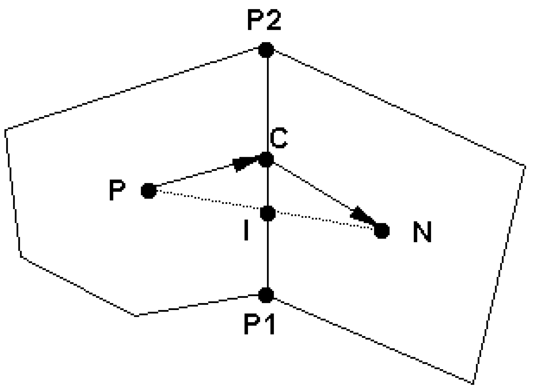
Sediment equation (12) and geophysical wave equation (21c) have the same form and are solved using the same finite-volume method described below. In the following, the sediment equation is used as an example with the size subscript k dropped for notation brevity. The sediment concentration (C) is located at the centroid of a polygonal mesh cell as illustrated in Figure 1 in which two cells are drawn (P and N). Gaussian integration of the equation over polygon P leads to the following discretized equation:
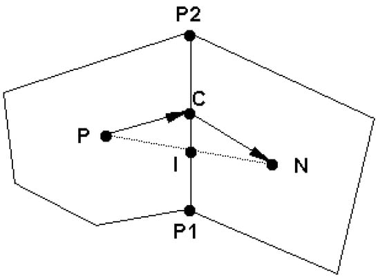
Figure 1.
Schematic illustrating a polygon P, one of its neighboring polygon N and other point locations (Source: [45]).
In the above, subscripts P and C refer to the points as in Figure 1; A is polygon area; is the velocity normal to the polygon side and at the side mid-point C; () is the unit normal vector of the polygon side; is the side length (distance from P1 to P2); and (, ) is the distance vector. In the remaining discussion, time superscript is dropped for ease of discussion.
Computation of concentration C at the side midpoint is carried out in two steps. First, the value at the intercept point I between lines PN and P1P2 in Figure 1 is computed by:
In the above, and , () is the distance vector from P to C and is C to N. Second, the concentration at the side midpoint C is computed as:
Third and final, the mid-point concentration used for sediment flux computation () is obtained by adding a damping term as:
where d is the amount of damping—a value of 0.2~0.3 is typically used (d = 0 means that the purely second-order scheme).
The discretized equation may be finally organized into the following linear equation form:
where “nb” refers to all neighboring polygons surrounding P and the coefficients are listed below:
The above linear equation is solved using the standard conjugate gradient solver with the ILU preconditioning.
2.5. Model Integeration
Integrated wave–current–sediment modeling has often been carried out using multiple sub-models with either explicit coupling and/or multiple meshes. The explicit multi-model coupling is less robust numerically and requires an external procedure for data exchange. Generic tools have been developed to manage the intricacies of when and how the sub-models are run, as well as data interpolation and exchange. For example, Earth System Modeling Framework (ESMF) was developed in [58], Open Modeling Interface (OpenMI) Environment in [59], and Modeling Coupling Toolkit (MCT) in [18].
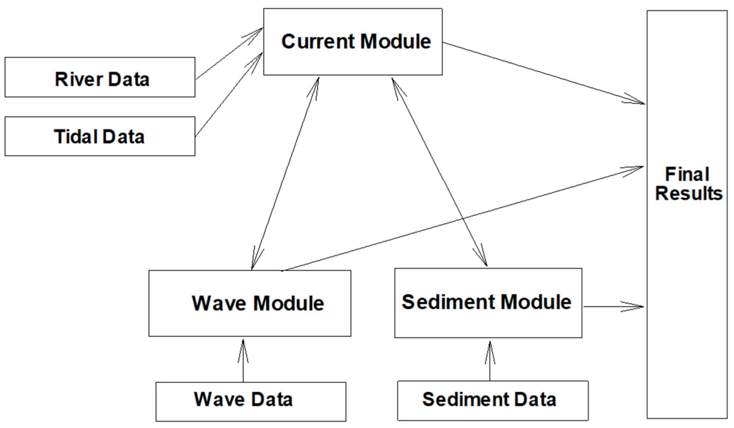
In this study, the wave–current–sediment integration is based on the one-model one-mesh approach. One model and one single unstructured mesh are used for all three sub-models. The three are coupled tightly within the same time step without using a separate coupling time interval for data exchanges as used in [29] for CCHE2D-Coast and [60] for Delft3D-SWAN. According to [60], the choice of the coupling time interval is not straightforward. The interval is often chosen to save computational time, rather than to represent the correct physical process. The effect of the applied coupling time interval on the accuracy of the model is questionable and has not been well studied. Figure 2 shows the diagram of the present current–wave–sediment integration workflow. Note that the “River Data” in the figure refers to the flow discharge and sediment rates from an upstream river—both water and sediment are delivered to an estuary area and can be included in the present model. Therefore, the present model can be used as river-only simulation, coast-only modeling or mixed simulation. The present modeling framework is linked to and may contribute toward the so-called watershed-coast system morpho-dynamics modeling as reviewed in [61].
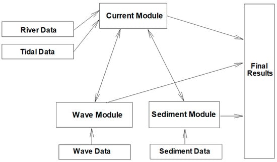
Figure 2.
A diagram illustrating the present integrated current–wave–sediment model and its coupling.
It is commented in passing that the “one model one mesh” approach is possible in SRH-Coast due to the fact that all governing equations of the three sub-models are solved in a time-accurate fashion. That is, the numerical method is truly unsteady and model solutions are valid at all times. A key advantage of such an approach is that it is most general, valid for both slow and fast processes and enhances stability as incremental changes may be controlled by the time step. A disadvantage is that the computing time can be large as the coupling interval time is not used and particularly if a user is interested in achieving only the final steady-state equilibrium sediment condition.
3. Model Verification and Validation
The new current–wave–sediment model is verified and validated in this section using three laboratory cases which have measured data for comparison.
3.1. Sediment Transport in a Trench with Wave Traveling along the Current
The first case is the sediment infilling and migration process in a trench under the combined flow and wave actions with the two in the same direction. The experimental case was reported by van Rijn [62]. The flume was a rectangle of 17 m in length and 0.3 m in width (see Figure 3a); the water depth was 0.5 m. A trench was created perpendicular to the flow direction and its initial geometry is shown in Figure 3b. The trench had a depth of 0.125 m, bottom width of 1.5 m and side slope of 1:10.
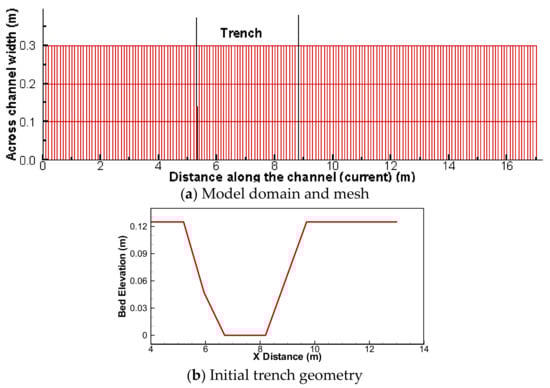
Figure 3.
Model domain, mesh and initial trench geometry for the van Rijn case.
A steady flow, with a velocity of 0.18 m/s and water depth of 0.255 m, was maintained. Regular waves were generated by a perforated wave paddle. The bed material consisted of fine sand with of 0.1 mm and had the measured fall velocity of 7.0 mm/s. To maintain the sediment equilibrium condition upstream of the trench, the same sand as the bed was supplied upstream at a constant rate of 0.0167 kg/m-s.
A 2D mesh is developed with a resolution of 0.1 m along the flume (170 cells) (Figure 3a). Main variables do not change across the flume so only three cells are used while the two sides are treated as symmetrical. Model inputs are based on the above measured data along with the following additional model parameters: (a) current flow Manning’s coefficient is 0.025; (b) waves have the significant wave height of 0.08 m and peak period of 1.5 s; and (c) the ripple roughness height of 1.45 mm is used to match the measured equilibrium sediment transport rate at the inlet.
The simulated sediment transport rate and trench morphological changes are compared with the measured data in Figure 4; good agreement is achieved. The main disagreement is the under-prediction of deposition at the upstream bank of the trench and over-prediction of erosion downstream. Among potential causes for the discrepancy, the transient nature of the ripples developed on the bed is the primary one. The ripple roughness height impacts both the current- and wave-induced shear stress and is found important. The results point to the future research need in obtaining the ripple roughness more accurately and dynamically. The modeling shows that the wave-induced shear stress for the sediment entrainment is 0.52 in terms of the Shields number, while the current-induced stress is 0.062. It suggests that the sediment movement is primarily driven by the waves for the case.
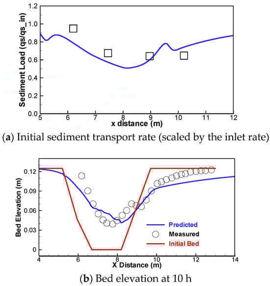
Figure 4.
Predicted (lines) and measured (symbols) initial sediment transport rate and the bed elevation at 10 h for the van Rijn case.
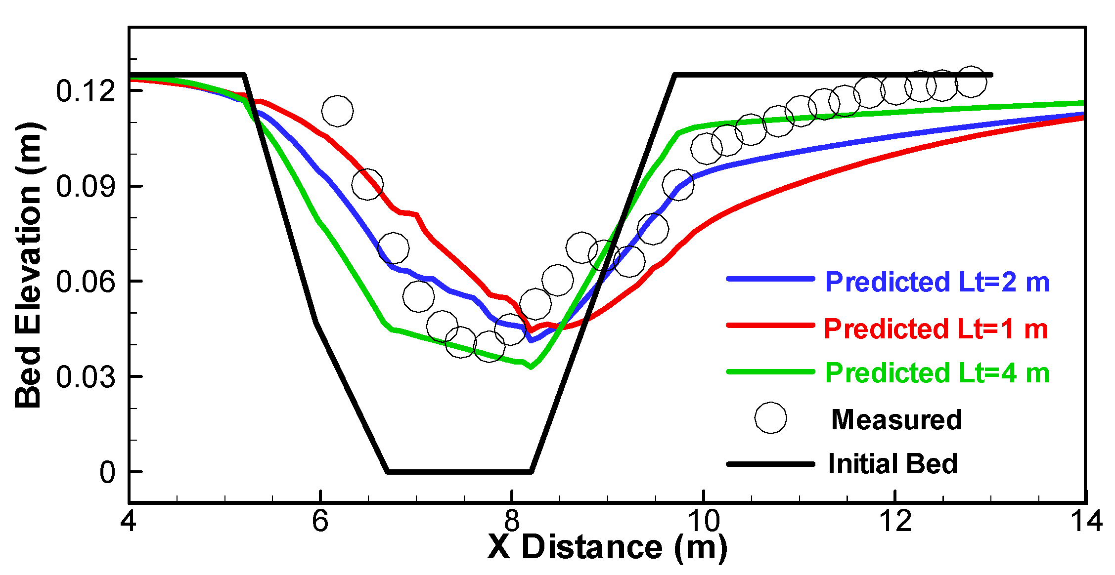
Among the sensitivity studies carried out to identify important input parameters, the adaptation length is singled out to be the most important and discussed further. Three adaptation lengths, 1.0 m, 2.0 m and 4.0 m, are used for the sensitivity study and the predicted trench bed morphology is compared in Figure 5. It is seen that the morphology is very sensitive to the adaptation length. Deposition on the upstream (left) bank increases with decreasing adaptation length, while erosion (migration) on the downstream (right) bank increases. This finding reflects the fact that the flow is highly unsteady and non-equilibrium sediment processes dominate. The results point to the importance of adopting the non-equilibrium sediment model as well as the need to develop an improved way to obtain the adaptation length for simulation.
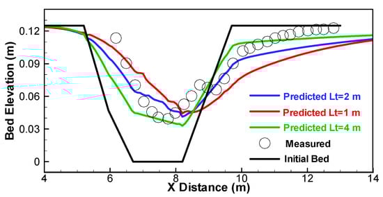
Figure 5.
Sensitivity of the trench morphological process to the adaptation length for the van Rijn case.
3.2. Sediment Transport in a Trench with Wave Propogating Normal to the Current
The second case is also a trench morphological evolution under the combined action of flow and wave, but the wave travels normally to the flow. The experiment of the case was carried out by Havinga [63] in a large basin at Delft Hydraulics and the results were summarized in [42]. The case labeled as T10-20-90 is selected for the present study.
The experimental basin is sketched in Figure 6a (see [63] for details]. An initial channel of 4.0 m in width was created in the basin using the guiding boards to confine the current flow within the channel. An initial trench was prepared across the channel—its centerline was 16.75 m from the flow entrance (not shown in Figure 6a). The trench had a bottom width of 0.5 m, top width of 3.5 m and depth of 0.2 m. During the experiment, clear waters entered the channel and an almost equilibrium sediment concentration was established before entering the trench. The current velocity across the channel was almost uniform; upstream of the trench, the average velocity was 0.246 m/s, the water depth was 0.419 m and the sediment transport rate was 0.0174 kg/m-s. The channel bed consisted of uniform sand with of 0.1 mm and fall velocity of 6.54 mm/s. Further, random waves were generated by a directional wave generator and propagated normally to the channel (or flow).
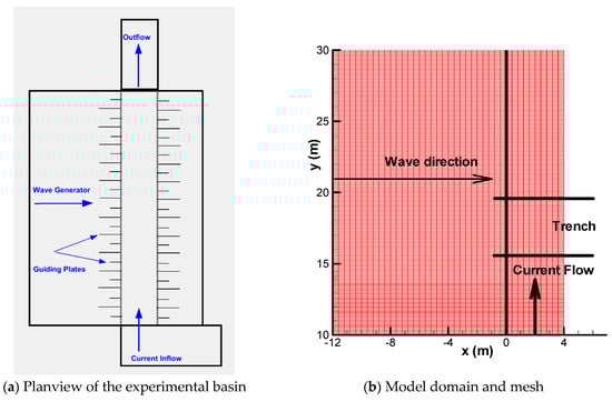
Figure 6.
Planview of the experimental basin and the numerical mesh for the Havinga case.
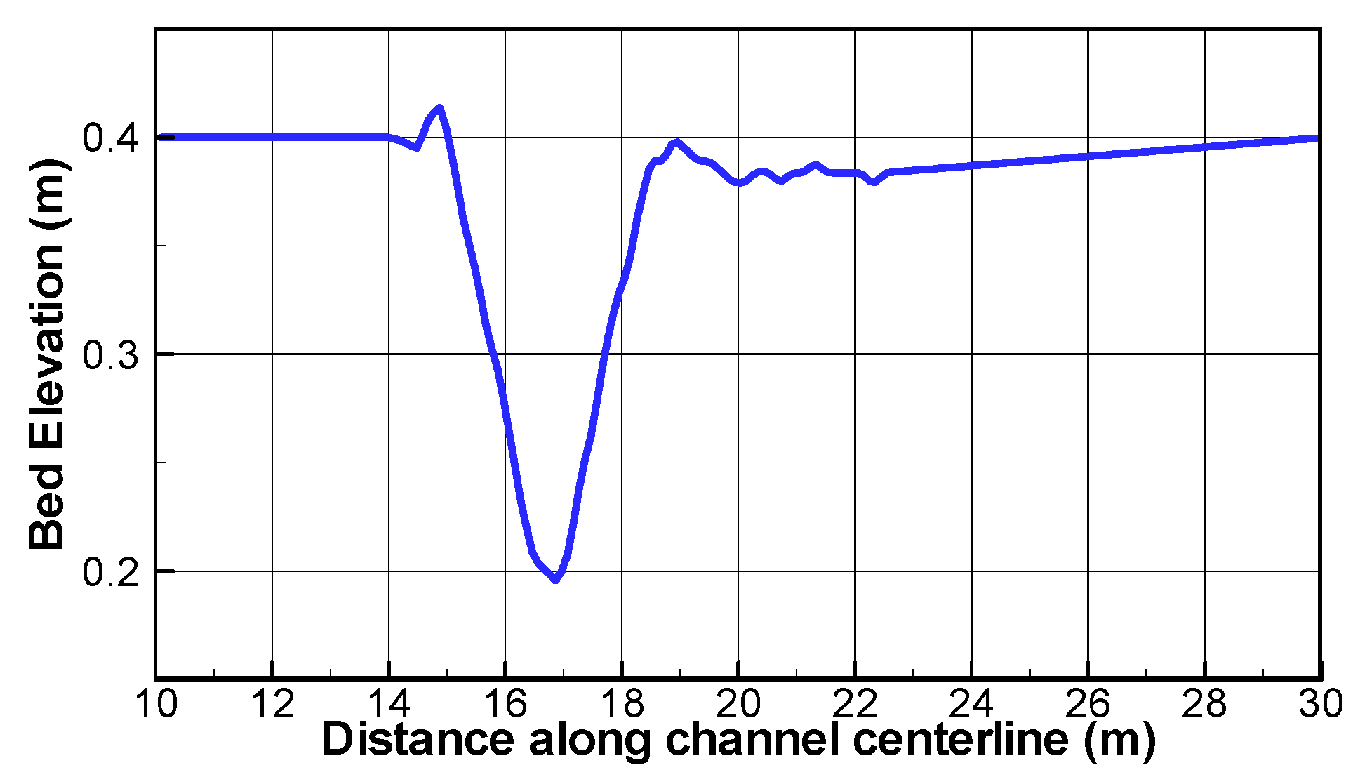
The model domain and mesh are shown in Figure 6b. The 16-by-20 m model domain is used to represent the basin and the channel is located on the right in Figure 6b. The mesh has a resolution of 0.1 m along the channel (200 mesh cells) and 0.4 m across the channel (40 cells). The channel bed profile along its centerline is shown in Figure 7. The trench profile at the beginning of the simulation is based on the measured data; the trench depth was approximately 0.2 m.
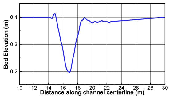
Figure 7.
The initial channel bed profile for the Havinga case.
Numerical model inputs are based mostly on the measured data stated above; additional model input parameters include (a) flow Manning’s coefficient is 0.02; (b) significant wave height is 0.105 m and wave peak period is 2.16 s; (c) bedform roughness height is 1.1 mm (determined such that the computed inlet sediment rate matches the measured value of 0.0174 kg/m-s); and (d) adaptation length is calibrated to be 2.0 m.
The simulated initial current velocity and significant wave height are plotted in Figure 8. As seen, the current is mostly confined within the channel and the diffusion onto the basin is small downstream of the trench. The flow creates a large but weak flow recirculation within the basin, which is negligible in modifying the wave field. The wave height is elevated on the upstream bank of the trench and reduced on the downstream bank.
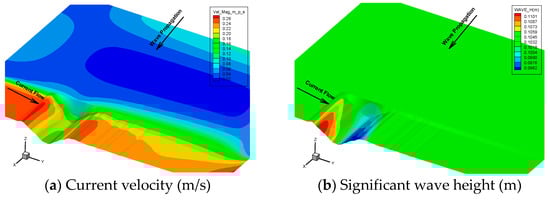
Figure 8.
Contours of the simulated current velocity and significant wave height at time 0 for the Havinga case.
The predicted trench morphological evolution is compared with the measured data in Figure 9. The model reproduces the observed trench morphology well. Main disagreement is at the downstream side of the trench bank—the bank erosion is under-predicted initially (e.g., at 8.3 h). Some discrepancy is also observed near the top of the upstream bank. As discussed for the first case, it may be attributed to the model inability to take into account the transient nature of the ripple-induced flow resistance and turbulence. Sensitivity studies confirm the same findings as the first case: both the bedform roughness and the model adaptation length are important mode inputs.
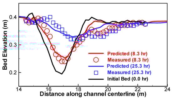
Figure 9.
Predicted and measured trench bed elevation at two times (8.3 h and 25.3 h) for the Havinga case.
3.3. Sediment Transport in a Beach Surf Zone
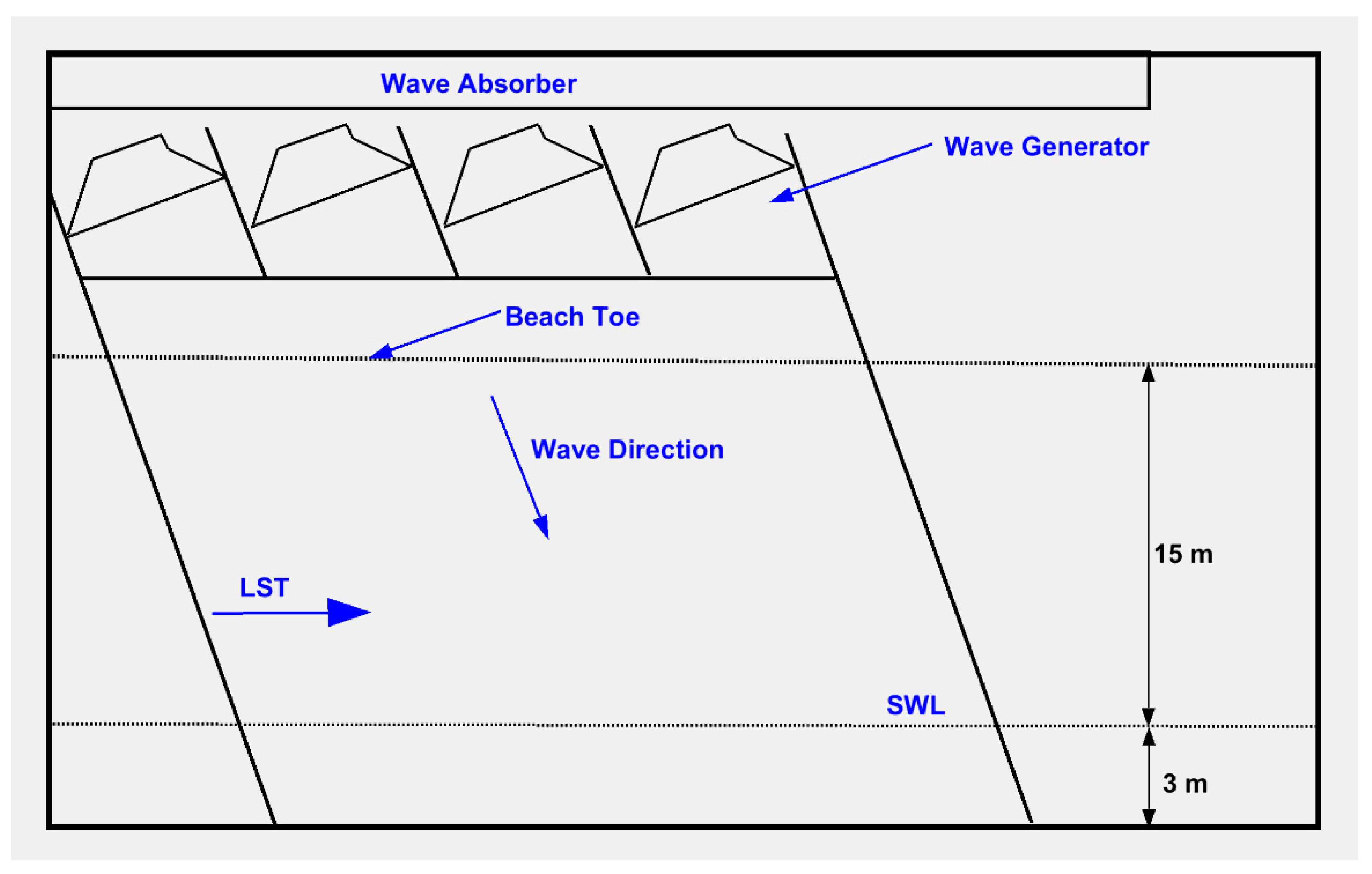
The third and final case is the wave–current–sediment dynamics in a beach surf zone typical of a near-shore coastal area. The case was experimentally studied using the Large-scale Sediment Transport Facility (LSTF) at the Coastal and Hydraulics Laboratory of the U.S. Army Engineer Research and Development Center in Vicksburg, Mississippi. The LSTF facility can generate oblique waves and produce uniform longshore currents and was described in [64,65] (see sketch in Figure 10).
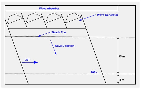
Figure 10.
Sketch of the LSTF flume for the Gravens-Wang case.
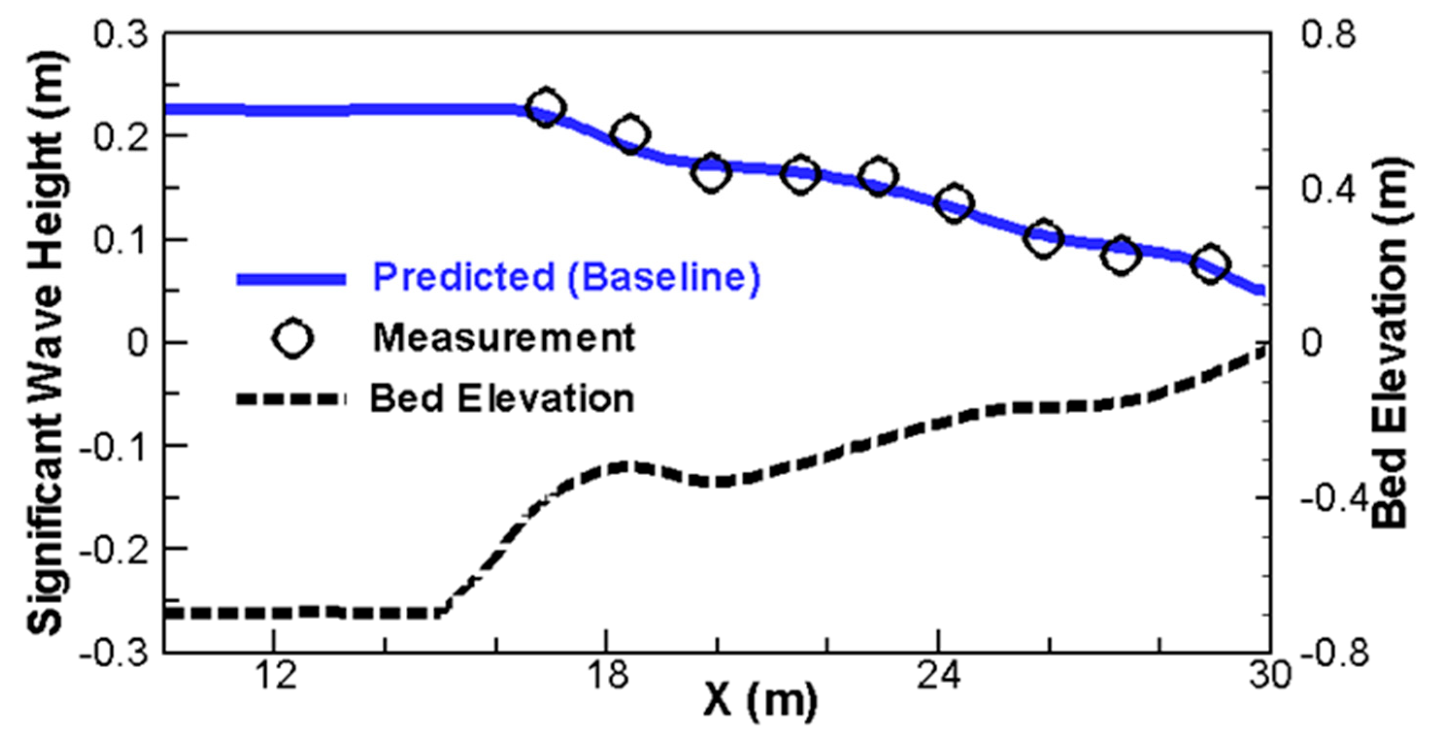
Five series of mobile-bed experiments were conducted and documented in [66,67]. Case 1 of the baseline series is chosen for the present numerical study. A uniform beach profile was constructed to represent a known equilibrium profile given the incident wave condition. Key experimental parameters are as follows [55]: (a) incident wave angle was 6.5o, significant wave height was 0.228 m and peak wave period was 1.465 s; (b) mean water level was −0.001 m; and (c) the flatbed portion on the offshore side had an elevation of −0.7 m.
The numerical model domain is shown in Figure 11. The domain has a longshore length of 120 m and cross-shore length of 30 m. The mesh has 160 cells along the shore and 100 cells cross the shore. The 18 m of the shore side represents the beach while 12 m of the offshore side implements the far-field waves entering the domain. The initial beach profile is based on the measured bed elevation and its contours are plotted in Figure 11.
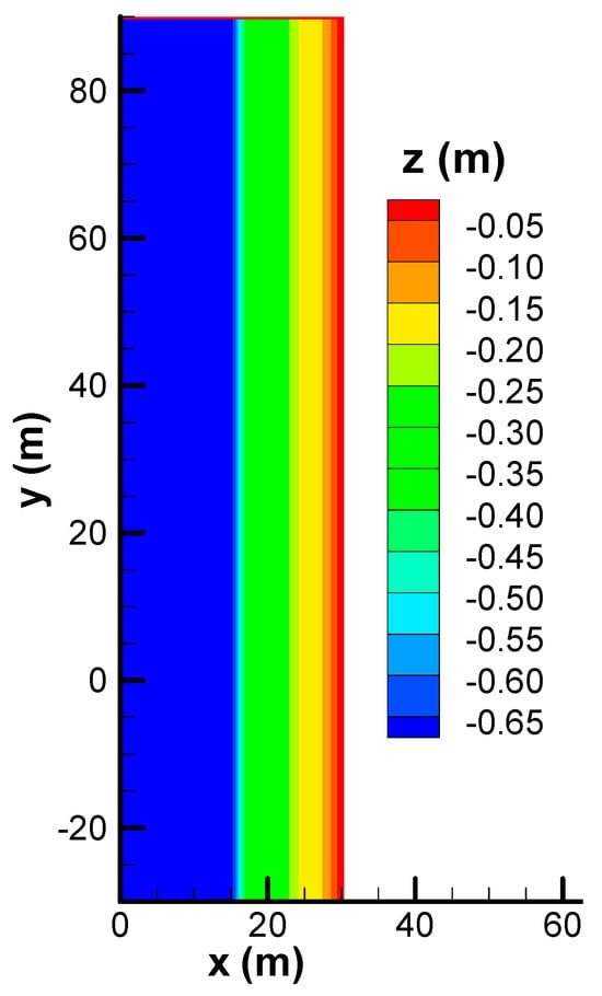
Figure 11.
Model domain and initial beach profile contours for the Gravens-Wang case.
Model inputs are based on the experimental data unless it is stated otherwise. Initially, the flow is quiescent with the water elevation at −0.001 m. The flow Manning’s coefficient is important for longshore current flows and calibrated to be 0.02. The oblique incident waves enter the domain from the offshore side and have the following properties: an incident angle of 6.5°, JONSWAP energy distribution and cos2s directional distribution. Several wave-induced processes are activated for the modeling. Wave breaking is a dominant process in beach surf zones and activated. Also active is the wave dissipation by bed friction. In addition, the radiation and surface-roller stresses are turned on as they are dominant in a beach surf zone having strong current–wave interactions. The beach bed consisted of well-sorted quartz sand with mm. The effective ripple roughness height is 10.0 mm and the adaptation length is 2.0 m—both are calibrated.
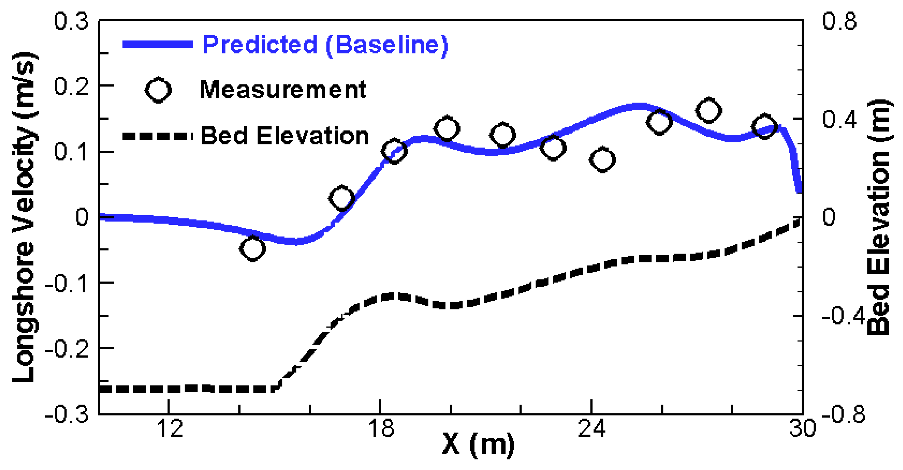
The model predicts well the significant wave height and wave-induced longshore current velocity in comparison with the data, as shown in Figure 12 and Figure 13. The longshore current is purely induced by the wave-induced radiation and surface roller stresses, verifying that the interaction processes are properly formulated and implemented. The measured longshore velocity showed three distinctive zones: negative velocity zone offshore (x < 17 m), peak #1 zone on the offshore side caused by the offshore bar (peak is around x = 20 m) and peak #2 on the shore side due to a small inshore bar. All three zones are predicted by the model except the location of peak #2.
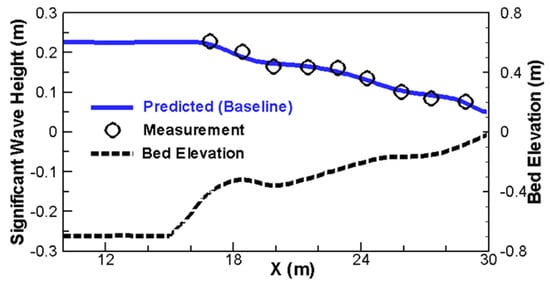
Figure 12.
Predicted and measured cross-shore distribution of the significant wave height for the Gravens-Wang case.
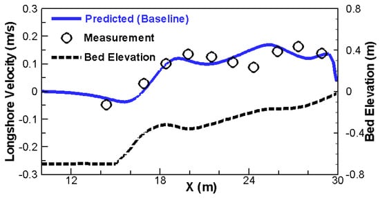
Figure 13.
Predicted and measured cross-shore distribution of the longshore current velocity for the Gravens-Wang case.
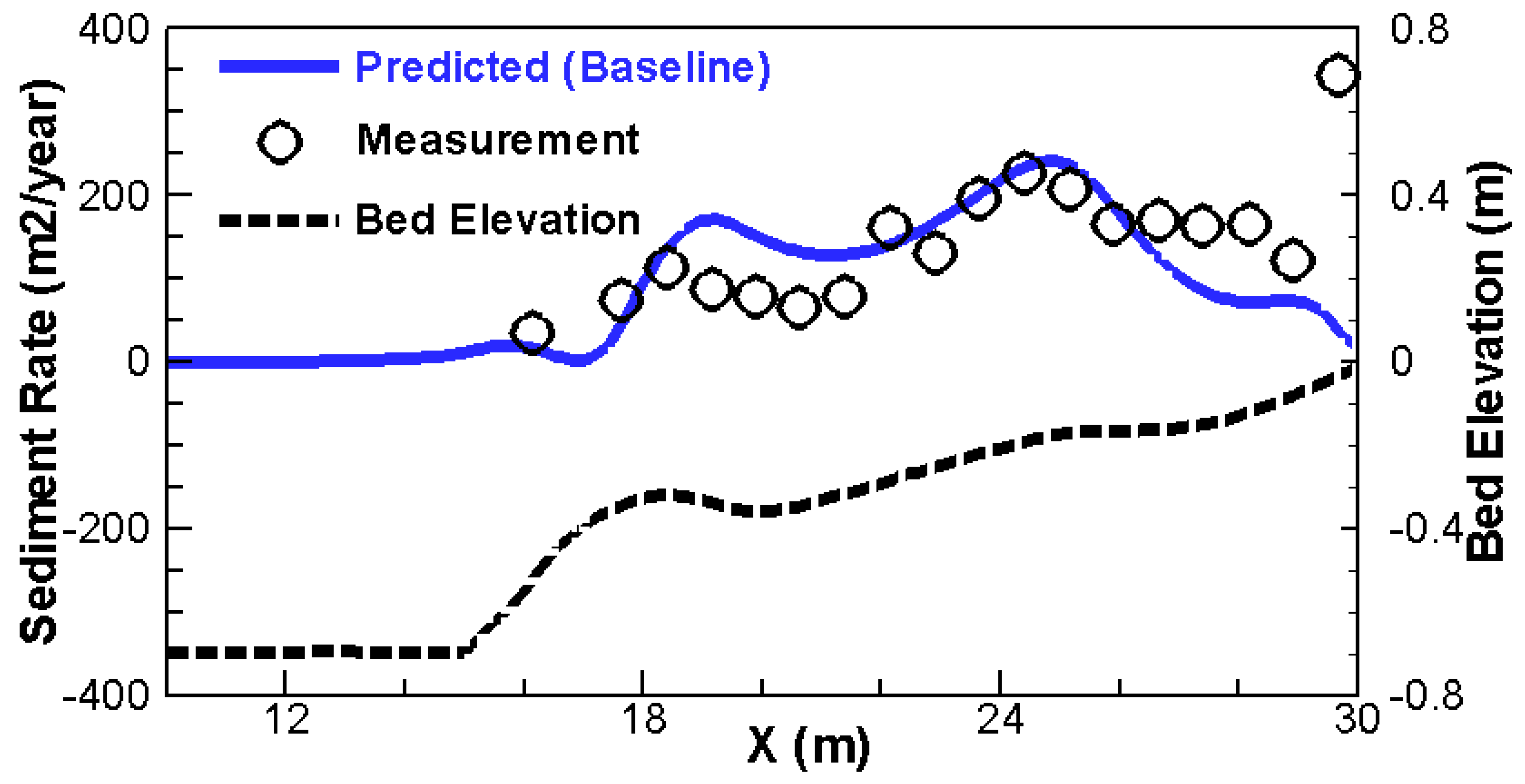
The longshore suspended load sediment rate is compared in Figure 14 and the result is also satisfactory. The two offshore sediment peaks observed in the experiment are predicted well by the model; even the locations of the two peaks are in agreement. There is an underprediction of the sediment rate in the so-called swash zone (x > 26 m). This discrepancy is expected according to [55]. The swash zone is very shallow and characterized by rapid oscillatory uprush and backwash motions which usually lead to much heightened sediment transport. This oscillatory sediment process in the swash zone is highly 3D in nature and not taken into consideration in the present 2D model.
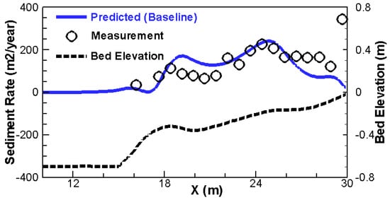
Figure 14.
Predicted and measured cross-shore distribution of the sediment transport rate for the Gravens-Wang case.
4. Concluding Remarks
In this study, a new integrated current–wave–sediment model is developed to advance the current models. A new contribution is the adoption of the one-model one-mesh strategy in which the three major sub-models—current flow, wave dynamics and sediment transport—are tightly integrated and a single unstructured mesh is adopted based on the most flexible mesh of the polygonal type. Another contribution is the development of a new sediment sub-model based on the non-uniform and non-equilibrium formulation and tailored for coastal applications under the combined influence of current flows and waves and their interactions.
The new integrated model has been tested and verified with an extensive list of test cases. In this paper, three verification and validation cases are presented and discussed. The model results are shown to match the experimental data satisfactorily.
Model sensitivity studies have also been carried out. It is shown that the most important model input parameters include the adaptation length of the non-equilibrium sediment process and the effective roughness height of the bedform. Both input parameters are probably not constant in natural settings and better empirical relations may need to be developed in the future to improve the model performance. It is also found that the flow roughness coefficient, i.e., the Manning’s coefficient, is another important model input, particularly for modeling the wave-induced longshore currents.
Funding
This research was funded by the Water Resources Agency, Taiwan.
Data Availability Statement
Dataset available on request from the authors.
Conflicts of Interest
The author declares no conflicts of interest.
References
- Amoudry, L.O.; Souza, A.J. Deterministic coastal morphological and sediment transport modeling: A review and discussion. Rev. Geophys. 2011, 49, RG2002. [Google Scholar] [CrossRef]
- Deng, J.; Woodroffe, C.D.; Roger, K.; Harff, J. Morphogenetic modelling of coastal and estuarine evolution. Earth Sci. Rev. 2017, 171, 254–271. [Google Scholar] [CrossRef]
- Sanchez, A.; Wu, W.; Beck, T.M. A depth-averaged 2-D model of flow and sediment transport in coastal water. Ocean Dyn. 2016, 66, 1475–1495. [Google Scholar] [CrossRef]
- Lu, Y.; Li, S.; Zuo, L.; Liu, H.; Roelvink, J.A. Advances in sediment transport under combined action of waves and currents. Int. J. Sediment. Res. 2015, 30, 351–360. [Google Scholar] [CrossRef]
- Klingbeil, K.; Lemarié, F.; Debreu, L.; Burchard, H. The numerics of hydrostatic structured-grid coastal ocean models: State of the art and future perspectives. Ocean Model. 2018, 125, 80–105. [Google Scholar] [CrossRef]
- Kim, H.S.; Lai, Y.G. Estuary and Coastal Modeling: Literature Review and Model Design; Technical Report No. ENV-2019-034; Technical Service Center, Bureau of Reclamation: Denver, CO, USA, 2019. [Google Scholar]
- Sanchez, A. An Implicit Finite-Volume Depth-Integrated Model for Coastal Hydrodynamic and Multiple-Sized Sediment Transport. Ph.D. Thesis, National Center for Computational Hydroscience and Engineering, The University of Mississippi, Oxford, MS, USA, 2013. [Google Scholar]
- Sorensen, O.R.; Kofoed-Hansen, H.; Rugbjerg, M.; Sorensen, L.S. A third-generation spectral wave model using an unstructured finite volume technique. In Proceedings of the Coastal Engineering Conference, Lisbon, Portugal, 19–24 September 2004; American Society of Civil Engineers: Reston, VA, USA, 2004; Volume 29, p. 894. [Google Scholar]
- Bellotti, G.; Franco, L.; Cecioni, C. Regional Downscaling of Copernicus ERA5 Wave Data for Coastal Engineering 561 Activities and Operational Coastal Services. Water 2021, 13, 859. [Google Scholar] [CrossRef]
- Lin, L.; Demirbilek, Z.; Mase, H.; Zheng, J.; Yamada, F. CMS-Wave: A Nearshore Spectral Wave Processes Model for Coastal Inlets and Navigation Projects; Technical Report ERDC/CHL TR-08-13; U.S. Army Engineer Research and Development Center, Coastal and Hydraulics Laboratory: Vicksburg, MS, USA, 2008. [Google Scholar]
- Ding, Y.; Zhang, Y.; Jia, Y. CCHE2D-Coast: Model Description and Graphical User Interface; NCCHE Technical Report; The University of Mississippi: Oxford, MS, USA, 2016; 88p. [Google Scholar]
- Booij, N.; Ris, R.C.; Holthuijsen, L.H. A third-generation wave model for coastal regions: 1. Model description and validation. J. Geophys. Res. 1999, 104, 7649–7666. [Google Scholar] [CrossRef]
- SWAN Team. SWAN Scientific and Technical Documentation Cycle III version 41.20AB; Technical and scientific documentation; Delft University of Technology: Delft, The Netherlands, 2019. [Google Scholar]
- Genseberger, M.; Donners, J. Hybrid SWAN for Fast and Efficient Practical Wave Modelling—Part 2. In Computational Science—ICCS 2020, Proceedings of the 20th International Conference, Amsterdam, The Netherlands, 3–5 June 2020; Krzhizhanovskaya, V.V., Zavodszky, G., Lees, M.H., Dongarra, J.J., Sloot, P.M.A., Brissos, S., Teixeira, J., Eds.; Lecture Notes in Computer Science; Springer: Cham, Switzerland, 2020; Volume 12139, p. 12139. [Google Scholar] [CrossRef]
- Lesser, G.R.; Roelvink, J.A.; van Kester, J.A.T.M.; Stelling, G.S. Development and validation of a three-dimensional morphological model. Coast. Eng. 2004, 51, 883–915. [Google Scholar] [CrossRef]
- van Rijn, L.C. Principles of Sediment Transport in Rivers, Estuaries, and Coastal Seas; Aqua Publications: Blokzil, The Netherlands, 1993; Available online: http://www.aquapublications.nl (accessed on 15 October 2020).
- van Ledden, M. Sand-Mud Segregation in Estuaries and Tidal Basins. Ph.D. Thesis, Delft University of Technology, Delft, The Netherlands, 2003. [Google Scholar]
- Warner, J.C.; Perlin, N.; Skyllingstad, E.D. Using the model coupling toolkit to couple earth system models. Environ. Model. Softw. 2008, 23, 1240–1249. [Google Scholar] [CrossRef]
- Luo, J.; Li, M.; Sun, Z.; O’Connor, B.A. Numerical modelling of hydrodynamics and sand transport in the tide-dominated coastal-to-estuarine region. Mar. Geol. 2013, 342, 14–27. [Google Scholar] [CrossRef]
- Dietrich, J.; Zijlema, M.; Westerink, J.; Holthuijsen, L.; Dawson, C.; Luettich, R., Jr.; Jensen, R.; Smith, J.; Stelling, G.; Stone, G. Modeling hurricane waves and storm surge using integrally-coupled, scalable computations. Coast. Eng. 2011, 58, 45–65. [Google Scholar] [CrossRef]
- Qi, J.; Jing, Y.; Chen, C.; Zhang, J. Numerical Simulation of Tidal Current and Sediment Movement in the Sea Area near Weifang Port. Water 2023, 15, 2516. [Google Scholar] [CrossRef]
- Christakos, K.; Björkqvist, J.V.; Tuomi, L.; Furevik, B.R.; Breivik, Ø. Modelling wave growth in narrow fetch geome-557 tries: The white-capping and wind input formulations. Ocean Model. 2021, 157, 101730. [Google Scholar] [CrossRef]
- Buttolph, A.M.; Reed, C.W.; Kraus, N.C.; Ono, N.; Larson, M.; Camenen, B.; Hanson, H.; Wamsley, T.; Zundel, A.K. Two-Dimensional Depth-Averaged Circulation Model CMS-M2D: Version 3.0, Report 2: Sediment Transport and Morphology Change; Technical Report, ERDC/CHL TR-06-9; Coastal and Hydraulics Laboratory, ERDC, US Army Corps of Engineers: Vicksburg, MS, USA, 2006. [Google Scholar]
- Mase, H. Multidirectional random wave transformation model based on energy balance equation. J. Coast. Eng. 2001, 43, 317–337. [Google Scholar] [CrossRef]
- Favaretto, C.; Martinelli, L.; Vigneron, E.M.P.; Ruol, P. Wave Hindcast in Enclosed Basins: Comparison among SWAN, STWAVE and CMS-Wave Models. Water 2022, 14, 1087. [Google Scholar] [CrossRef]
- Nassar, K.; Masria, A.; Mahmod, W.E.; Negm, A.; Fath, H. Hydro-morphological modeling to characterize the adequacy of jetties and subsidiary alternatives in sedimentary stock rationalization within tidal inlets of marine lagoons. Appl. Ocean Res. 2019, 84, 92–110. [Google Scholar] [CrossRef]
- Mera, M.; Chrisnatilova, D. Numerical Simulation to Determine the Effectiveness of Groynes and Breakwaters as Protective Structures for Gandoriah Beach, Pariaman City. IOP Conf. Ser. Mater. Sci. Eng. 2021, 1041, 012001. [Google Scholar] [CrossRef]
- Lin, L.; Demirbilek, Z.; Thomas, R.C.; Rosati, J. Verification and Validation of the Coastal Modeling System; Report 2: 572 CMS-Wave; U.S. Army Engineer Research and Development Center, Coastal and Hydraulics Laboratory: Vicksburg, MS, USA, 2011. [Google Scholar]
- Ding, Y.; Wang, S.S.Y. Development and Application of a Coastal and Estuarine Morphological Process Modeling System. J. Coast. Res. 2010, 10052, 127–140. [Google Scholar] [CrossRef]
- Ding, Y.; Kuiry, S.; Elgohry, M.; Jia, Y.; Altinakar, M.S.; Yeh, K.-C. Impact assessment of sea-level rise and hazardous storms on coasts and estuaries using integrated processes model. Ocean Eng. 2013, 71, 74–95. [Google Scholar] [CrossRef]
- Ding, Y.; Yeh, K.-C.; Wei, S.-T. Integrated coastal process modeling and impact assessment of floating and sedimentation in coasts and estuaries. Coast. Eng. Proc. 2017, 1, 18. [Google Scholar] [CrossRef]
- Hsieh, T.-C.; Ding, Y.; Yeh, K.-C.; Jhong, R.K. Investigation of Morphological Changes in the Tamsui River Estuary Using an Integrated Coastal and Estuarine Processes Model. Water 2020, 12, 1084. [Google Scholar] [CrossRef]
- Jia, Y.; Wang, S.S.Y. CCHE2D: Two-Dimensional Hydrodynamics and Sediment Transport Model for Unsteady Open Channel Flows over Loose Bed; Technical Report No. NCCHE-TR-2001-1; National Center for Computational Hydroscience and Engineering, The University of Mississippi: Oxford, MS, USA, 2001. [Google Scholar]
- Lai, Y.G. Two-Dimensional Depth-Averaged Flow Modeling with an Unstructured Hybrid Mesh. J. Hydraul. Eng. 2010, 136, 12–23. [Google Scholar] [CrossRef]
- Lai, Y.G.; Kim, H.S. A Near-Shore Linear Wave Model with the Mixed Finite Volume and Finite Difference Unstructured Mesh Method. Fluids 2020, 5, 199. [Google Scholar] [CrossRef]
- Eisma, D.; Ji, Z.; Chen, S.; Chen, M.; van der Gaast, S.J. Clay Mineral Composition of Recent Sediments along the China Coast, in the Yellow Sea and the East China Sea; NIOZ-Rapport 1995-4; Nederlands Instituut voor Onderzoek der Zee: Den Burg, The Netherlands, 1995. [Google Scholar]
- Wu, W. Computational River Dynamics; Taylor and Francis: Abingdon, UK, 2008. [Google Scholar]
- Pope, S.B. Turbulent Flows; Cambridge University Press: Cambridge, UK, 2000. [Google Scholar]
- Rodi, W. Turbulence Models and Their Application in Hydraulics. A State-of-the-Art Review. IAHR Monograph, 3rd ed.; Balkema: Zutphen, The Netherlands, 1993. [Google Scholar]
- Tolman, H.L. A third-generation model for wind waves on slowly varying, unsteady, and inhomogeneous depths and currents. J. Phys. Oceanogr. 1991, 21, 782–797. [Google Scholar] [CrossRef]
- Holthuijsen, L.H. Waves in Oceanic and Coastal Waters; Cambridge University Press: Cambridge, UK, 2007. [Google Scholar]
- van Rijn, L.C.; Havinga, F.J. Transport of fine sands by currents and waves. II. J. Waterw. Port Coast. Ocean Eng. 1995, 121, 123–133. [Google Scholar] [CrossRef]
- van Rijn, L.C. Unified view of sediment transport by currents and waves, I: Initiation of bed motion, bed roughness, and bed-load transport. J. Hydraul. Eng. ASCE 2007, 133, 649–667. [Google Scholar] [CrossRef]
- Miller, M.C.; McCave, I.N.; Komar, P.D. Threshold of sediment motion under unidirectional current. Sedimentology 1977, 24, 507–527. [Google Scholar] [CrossRef]
- Lai, Y.G. A Two-Dimensional Depth-Averaged Sediment Transport Mobile-Bed Model with Polygonal Meshes. Water 2020, 12, 1032. [Google Scholar] [CrossRef]
- Johnson, H.K.; Zyserman, J.A. Controlling spatial oscillations in bed level update schemes. Coast. Eng. 2002, 46, 109–126. [Google Scholar] [CrossRef]
- Soulsby, R.L. Dynamics of Marine Sands: A Manual for Practical Applications; Thomas Telford Publications: London, UK, 1997. [Google Scholar]
- van Rijn, L.C. Unified view of sediment transport by currents and waves, II: Suspended transport. J. Hydraul. Eng. ASCE 2007, 133, 668–689. [Google Scholar] [CrossRef]
- Gaeuman, D.; Sklar, L.; Lai, Y.G. Flume experiments to constrain bedload adaptation length. J. Hydrol. Eng. 2014, 20, 1–5. [Google Scholar] [CrossRef]
- Bayram, A.; Larson, M.; Miller, H.C.; Kraus, N.C. Cross-shore distribution of longshore sediment transport: Comparison between predictive formulas and field measurements. Coast. Eng. 2001, 44, 79–99. [Google Scholar] [CrossRef]
- Camenen, B.; Larroude, P. Comparison of sediment transport formulae for the coastal environment. Coast. Eng. 2003, 48, 111–132. [Google Scholar] [CrossRef]
- Camenen, B.; Larson, M. A general formula for non-cohesive bed load sediment transport. Estuar. Coast. Shelf Sci. 2005, 63, 249–260. [Google Scholar] [CrossRef]
- Camenen, B.; Larson, M. A Unified Sediment Transport Formulation for Coastal Inlet Application; Technical Report ERDC/CHL CR-07-1; US Army Engineer Research and Development Center: Vicksburg, MS, USA, 2007. [Google Scholar]
- Camenen, B.; Larson, M. A general formula for noncohesive suspended sediment transport. J. Coast. Res. 2008, 24, 615–627. [Google Scholar] [CrossRef]
- Nam, P.T.; Larson, M.; Hanson, H.; Hoan, L.X. A numerical model of nearshore waves, currents, and sediment transport. Coast. Eng. 2009, 56, 1084–1096. [Google Scholar] [CrossRef]
- Hsu, T.W.; Ou, S.H.; Liau, J.M.; Zanke, U.; Roland, A.; Mewis, P. Development and implement of a spectral finite element wave model. In Proceedings of the 5th International Symposium on Wave Measurement and Analysis, Madrid, Spain, 3–7 July 2005. [Google Scholar]
- Hsu, T.W.; Ou, S.H.; Liau, J.M. Hindcasting nearshore wind waves using a FEM code for SWAN. Coast. Eng. 2005, 52, 177–195. [Google Scholar] [CrossRef]
- Collins, N.; Theurich, G.; Deluca, C.; Suarez, M.; Trayanov, A.; Balaji, V.; Li, P.; Yang, W.; Hill, C.; Da Silva, C. Design and implementation of components in the earth system modeling framework. Int. J. High Perform. Comput. Appl. 2005, 19, 341–350. [Google Scholar] [CrossRef]
- Gregersen, J.B.; Gijsbers, P.J.A.; Westen, S.J.P.; Blind, M. OpenMI: The essential concepts and their implications for legacy software. Adv. Geosci. 2005, 4, 37–44. [Google Scholar] [CrossRef]
- Cats, G. Numerical Modeling of Wave-Current Interaction with the Use of a Two-Way Coupled System. Master’s Thesis, Delft University of Technology, Delft, The Netherlands, 2014. [Google Scholar]
- Samaras, A.G. Towards integrated modelling of Watershed-Coast System morphodynamics in a changing climate: A critical review and the path forward. Sci. Total Environ. 2023, 882, 163625. [Google Scholar] [CrossRef]
- van Rijn, L.C. Sedimentation of dredged channels by currents and waves. J. Waterw. Port Coast. Ocean Eng. 1986, 112, 541–559. [Google Scholar] [CrossRef]
- Havinga, F.J. Sediment Concentrations and Transport in Case of Irregular Non-Breaking Waves with a Current. Master’s Thesis, Delft University of Technology, Delft, The Netherlands, 1992. Rep. H840 Parts E, F, G.. [Google Scholar]
- Hamilton, D.G.; Ebersole, B.A. Establishing uniform longshore currents in a large-scale sediment transport facility. Coast. Eng. 2001, 42, 199–218. [Google Scholar] [CrossRef]
- Wang, P.; Ebersole, B.A.; Smith, E.R.; Johnson, B.D. Temporal and spatial variations of surf-zone currents and suspended sediment concentration. Coast. Eng. 2002, 46, 175–211. [Google Scholar] [CrossRef]
- Gravens, M.B.; Wang, P.; Kraus, N.C.; Hanson, H. Physical model investigation of morphology development at headland structures. In Proceedings of the 30th International Conference on Coastal Engineering, San Diego, CA, USA, 3–8 September 2006; World Scientific Press: San Diego, CA, USA, 2006; pp. 3617–3629. [Google Scholar]
- Gravens, M.B.; Wang, P. Data Report: Laboratory Testing of Longshore Sand Transport by Waves and Currents. In Morphology Change Behind Headland Structures; Geology Faculty Publications: Tampa, FL, USA, 2007; Volume 258, Available online: https://scholarcommons.usf.edu/gly_facpub/258 (accessed on 15 March 2021).


Disclaimer/Publisher’s Note: The statements, opinions and data contained in all publications are solely those of the individual author(s) and contributor(s) and not of MDPI and/or the editor(s). MDPI and/or the editor(s) disclaim responsibility for any injury to people or property resulting from any ideas, methods, instructions or products referred to in the content. |
© 2024 by the author. Licensee MDPI, Basel, Switzerland. This article is an open access article distributed under the terms and conditions of the Creative Commons Attribution (CC BY) license (https://creativecommons.org/licenses/by/4.0/).