Modeling Rainfall Impact on Slope Stability: Computational Insights into Displacement and Stress Dynamics

Abstract

The susceptibility of loess slopes to collapses, landslides, and sinkholes is a global concern. Rainfall is a key factor exacerbating these issues and affecting slope stability. In regions experiencing significant infrastructure and urban growth, understanding and mitigating rainfall effects on loess landslides is crucial. ADINA numerical software 9 was utilized to explore rain-induced erosion’s influence on landslide dynamics. The simulations were based on local rainfall trends. The rainfall intensities examined were as follows: 200 mm/day, 300 mm/day, and 400 mm/day. The results indicate a pronounced impact of rainfall intensity on both the movement and stress levels within the slope. Higher rainfall intensities lead to increased movement and a wider stress impact area at the base of the slope. It was observed that surface movement is minimal at the slope crest but increases towards the bottom, with the greatest movement seen at the slope’s base.

1. Introduction

Loess slope landslide poses a threat to human lives and properties [1,2]. It is estimated that about a third of China’s landslide disasters occur in loess regions, with 1131 in Shaanxi Province alone. Landslides are a recurring global natural disaster that often causes widespread destruction, killing tens of thousands of people and causing economic losses of billions of dollars every year. Their severity exceeds the natural disasters. Among the various external factors that lead to loess slope landslide, rainfall is the main trigger factors [3,4].

According to relevant reports, rainfall-induced landslides can be attributed to the following three primary factors: (1) decreased cohesion of slope rock and soil; (2) increased weight of rocks and soil; and (3) elevated slope sliding force. In a study conducted by Wang et al. [5], a field investigation was carried out on loess slopes that experienced prolonged heavy rainfall. The findings revealed a strong correlation between the occurrence of loess flow landslides and factors such as rainfall intensity and loess strength. Xu et al. [6] performed stress path testing on undisturbed samples to examine the relationship between groundwater level rise and soil behavior. The study revealed that an elevation in pore pressure can result in soil liquefaction, ultimately culminating in landslides. To investigate the impact of rainfall on loess landslides, Chen et al. [7] performed cloud seeding tests on natural loess slopes. The purpose was to study the deformation patterns of loess landslides triggered by shear forces. Huang et al. [8] conducted indoor cloud seeding erosion model tests [8] considering the effects of gravel content and rainfall intensity on slope surface erosion. The authors also examined the forms of erosion damage, runoff rate, infiltration rate and scouring materials of clay slopes. Wang et al. [9] conducted an indoor experiment using artificial simulated rainfall to quantify the erosion response of microtopography on both sandy and loess slopes. They utilized three-dimensional laser scanning technology to analyze the slope microtopography and soil erosion. Sun et al. [10] focused on typical examples and developed a landslide disaster resistance mapping model induced by rainfall on mountain slopes, taking into account historical slope damage records and condition factor data mining. A new and more reliable LR evaluation model for slope disaster resistance was proposed.

Numerical simulation is a novel approach for simulating landslides, and numerous scholars have employed this method to conduct landslide simulation experiments and compare the results with on-site tests [11,12,13]. Arbanas [14] utilized the strength reduction method to perform a numerical analysis on slopes, aiming to determine the shape of the fracture zone. Furthermore, Mingtao [15] comprehensively discussed the characteristics of accumulated landslides and extensively explored the impact of rainfall and groundwater on the stability of such landslides. Taking the Baolingsi landslide as a representative case, a numerical simulation was carried out using FLAC 2D software to analyze the impact of the groundwater and rainfall on the stability of the landslide. Zhong [16] developed a numerical model to simulate the coupling process of water–soil in dam failures. This model specifically focuses on the evolution of collapse morphology during the failure process, aiming to enhance the accuracy of collapse process prediction. Additionally, the model is capable of considering unilateral and bilateral erosion, as well as incomplete and basal erosion in the vertical direction. Fan [17] began by utilizing the fundamental equation of landslide movement and proceeded to establish a numerical model for landslide motion through calculus transformation of the differential equation, followed by numerical discretization. This numerical model was then applied to calculate and analyze several representative analysis examples as well as actual landslides. In addition, the deterministic block theory [18], probability estimation methods [19] and random parameters distributions [20] are also widely used in the stability analysis of slopes.

In this research, the ADINA finite element analysis tool is selected to model the movement of a slope when subjected to the rainfall rate of 274 mm/d, drawing on data acquired from field monitoring. Additionally, this study replicates the conditions of slope slippage under various precipitation scenarios, including natural rain levels as well as specific rates of 200, 300, and 400 mm/d. This investigation integrates findings from simulations of slope stress, displacement, and vector alterations at these different precipitation rates to thoroughly examine the behavior of loess slopes in response to rainfall-induced changes.

2. Software and Methods

ADINA software 9 excels in addressing both linear and nonlinear challenges. Utilizing the incremental method, a numerical strategy for managing nonlinear physical complexities, ADINA effectively navigates these issues [21,22,23]. It adjusts the incremental step, typically by modifying load or time increments, to closely mimic the actual solution during the simulation. The applications of engineering simulations of ADINA are vast, spanning various sectors such as civil, geotechnical, and underground engineering.

2.1. Model and Parameter

2.1.1. Assumptions

The following basic assumptions have been made [24,25,26]:

(1)

We model the slope as a stratified system, with each layer exhibiting uniform properties but differing from others. These layers, isotropic within themselves, maintain tight inter-layer connections.

(2)

In this model, soil granules are treated as non-compressible entities.

(3)

As the rainfall intensity heightens, the shear strength of the topsoil layer diminishes, modeled over 70 incremental time steps.

(4)

The soil up to a depth of 3.0 m is assumed to be fully saturated. For this portion, we adopt the saturated soil density as its defining parameter.

(5)

We opt for a 2D Solid element in our simulations, specifically choosing the ‘Plane Structure’ as the Element Sub Type and ‘Porous Media’ for the Material Type.

2.1.2. Calculation Model

The computational framework is structured around four primary components: the material behavior model, spatial design, limit conditions, and soil attribute determination. The elastic–plastic material behavior model is built on three critical postulates. The selection of an appropriate yield criterion is vital as it profoundly influences the computed outcomes of the plastic region. Distinct yield criteria lead to the formulation of varying elastic–plastic models.

(1) Model

The M-C criterion describes the relationship between $\tau$ (shear stress) and $\sigma$ (normal stress). It reflects the basic characteristics of soil’s frictional strength as the loose material and is widely used due to its simplicity, practicality, and ease regarding obtaining material strength parameters. In the Mohr–Coulomb strength theory, the stress plane is represented by a straight line.

$${\tau }_{ }=c+\sigma \tan \phi$$

(1)

$${\sigma }_3-{\sigma }_1=\frac{1}{1-\sin \varphi }(C\cos \varphi +{\sigma }_3\sin \varphi )$$

(2)

But in the principal stress space, the yield surface of Mohr–Coulomb is pyramid-shaped, and in the π plane, it takes the form of an irregular hexagon. When ${\sigma }_1>{\sigma }_2>{\sigma }_3$, its yield function can be expressed as follows:

$$F=\frac{1}{2}({\sigma }_3-{\sigma }_1)+\frac{1}{2}({\sigma }_3+{\sigma }_1)\sin \varphi -\cos \varphi =0$$

(3)

In this context, $\tau$ is indicative of the shear strength, measured in kilopascals (kPa). Meanwhile, $\sigma$ is a reference to the normal stress, also quantified in kilopascals. The term c is utilized to denote the cohesive force, expressed in the same unit, kPa. The symbol φ is used to signify the internal friction angle, measured in degrees (°). The yield surface function is represented by $F$, and the symbols ${\sigma }_1$ and ${\sigma }_3$ are employed to depict the minimum and maximum principal stresses, respectively, each quantified in kilopascals.

Flow criterion: In stable materials, it is necessary for the plastic work to be greater than zero. The plastic work is expressed as follows:

$$d{\epsilon }_{ij}^{p}d{\sigma }_{ij}\ge 0$$

(4)

$$\frac{\partial g}{\partial {\sigma }_{ij}}d{\sigma }_{ij}>0$$

(5)

$$d{\epsilon }_{ij}^p=\lambda \frac{\partial g}{\partial {\sigma }_{ij}}$$

(6)

(2) Parameters of soil layers

The selection of soil parameters is shown in [27].

(3) ADINA Computational Numerical Simulation Process

①

Geometric modeling steps: We start by creating geometric models, beginning with the most basic elements (points) and expanding them into more complex forms (surfaces). Specifically, this involves modeling the root site’s dimensions as captured in the ADINA-Structure software 9.

②

Establishing boundary conditions: this involves specifying the constraints and conditions that define how the model interacts with its surroundings.

③

Load application: Here, we apply different types of loads to the model. This includes the application of pore flow loads along specified areas. Additionally, we apply loads that are proportional to the mass on the slope.

④

Material properties and group selection: In this step, we choose the appropriate materials and their properties. We then designate the 2D Solid unit for structural analysis, with specific sub-types and materials, including Plane Structure for element sub-types and Porous Media for the material type. The parameters for each group are defined as per the guidelines in [27].

⑤

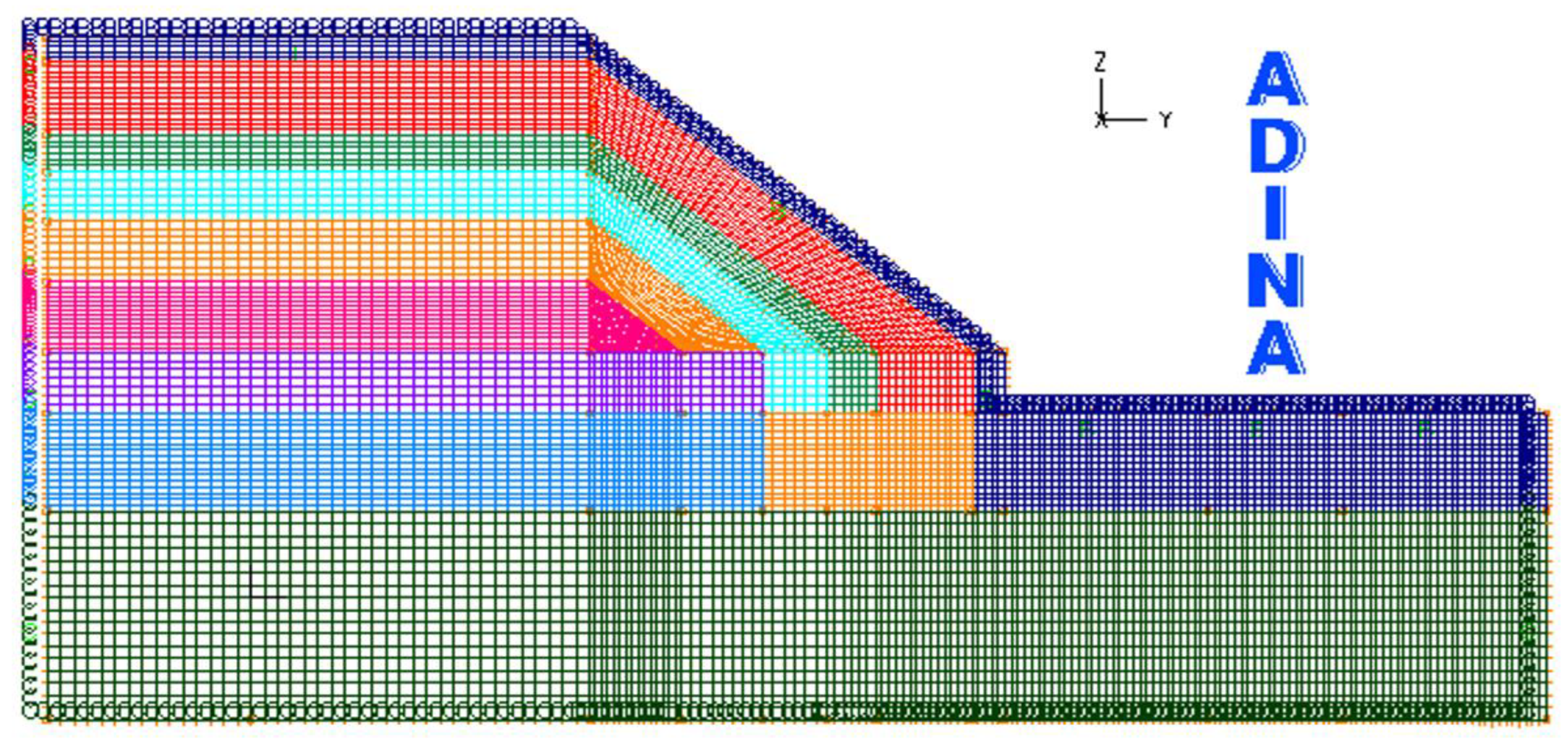
Grid partitioning: finally, we divide the model into a grid, as illustrated in Figure 1. This grid helps in detailed analysis and simulation.

Figure 1 shows the grid division.

2.1.3. Working Condition

The slope deformation under a rain intensity of 200, 274, 300, 400 mm/d is simulated.

3. Numerical Simulation Analysis

Based on on-site test data, the focus was on simulating the displacement of slope under a rainfall intensity of 274 mm/d, and then simulating the slope characteristics under a rainfall intensity of 200, 300, 400 mm/d.

3.1. Monitoring Data

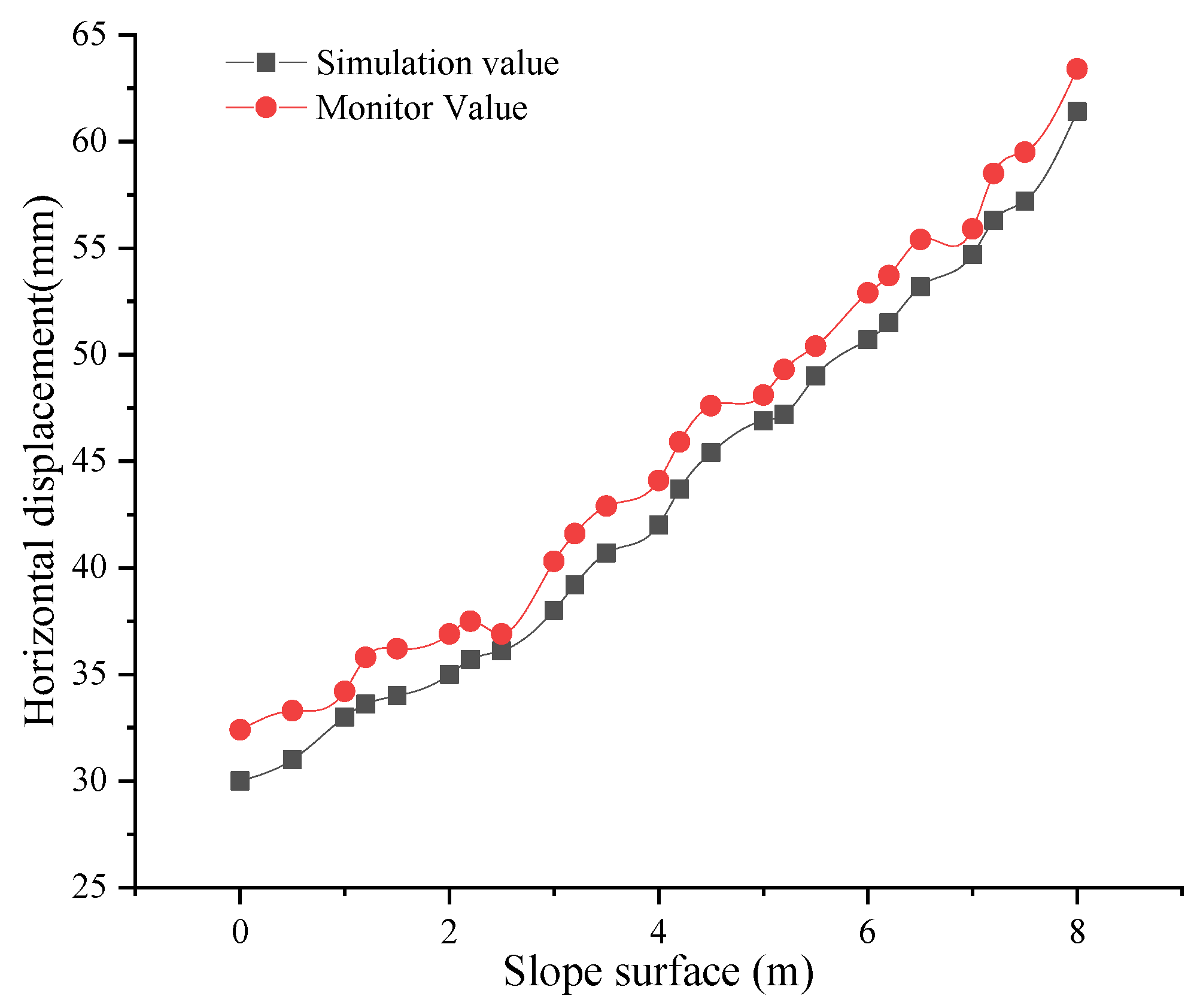
3.1.1. Rainfall Intensity of 274 mm/d

The stress, displacement, slope vector cloud map of the slope under the rainfall intensity of 274 mm/d are shown in Figure 2.

(1) Changes in the Stress

Figure 2a reveals that the stress at the surface of the slope is relatively low, and some areas experience tensile stress in the soil. The maximum stress zone is located at the slope’s foot, and the stress gradually increases from the surface to the slope bottom.

(2) Changes in the Displacement

Figure 2b shows the slope horizontal displacement. As can be seen from the figure, the horizontal displacement gradually increases at 274 mm/d of rainfall. The maximum displacement, reaching 60.22 mm, occurs within 1.5 m from the slope’s foot. The horizontal displacement at the slope’s top is relatively small, while the slope bottom is basically unaffected. Figure 2c shows a gradual decrease in vertical displacement from the top to the slope bottom. The maximum displacement of the slope’s top is 64.86 mm, and the displacement of the slope’s foot is relatively small. In the range of slope’s foot 1.0 m, the displacement is zero. In the slope combination displacement diagram of Figure 2d,e, the slope displaces more than 60 mm along the 1.5 m range of its surface, with the largest displacement occurring at the slope’s foot (81.39 mm), followed by the displacement at the top. The smallest displacement is observed at the slope crest. According to the displacement contour map in Figure 2e, it can be determined that the maximum slip zone is located in two arcs centered on the top and bottom of the slope, with radii of 8.0 m and 2.5 m, respectively. The displacement in this area is more than 20 mm.

(3) Changes in Strain Vector

It can be observed in Figure 2f that the stress at the slope’s foot is highest, corresponding to the highest strain. The lower part of the slope experiences tensile stress, indicated by positive strain vectors. The stress vector at the slope surface deviates downward, while the strain vector at the foot of the slope deviates approximately horizontally from the foot. Consequently, the slope body undergoes diagonal sliding downwards along the surface of the slope.

3.1.2. Comparative Analysis

(1) Slope Displacement

Figure 3 illustrates the relationship curve between the measured horizontal displacement and the simulated horizontal displacement under the 274 mm/d rainfall intensity.

It can be observed (in Figure 3) that the simulated horizontal displacement value is smaller than the measured value. However, as we move further down the slope, the measured value gradually approaches the simulated value, and near the slope’s foot, the simulated value aligns well with the measured value.

(2) Changes in internal displacement of slope

The 0 # hole is situated on top platform, positioned 1.0 m away from the slope’s top. The 1–5 # measuring holes are located on the slope surface, with distances of 2.0, 4.0, 6.0, and 8.0 m from the slope’s top. Lastly, the 5 # hole is situated at the slope’s foot. Figure 3 shows the schematic diagram of sensor embedding points.

Figure 4 illustrates the displacement time curves at various depths of the 0–5 measuring holes on the slope under the influence of 274 mm/d rainfall intensity.

By analyzing the displacement changes in the six measuring holes, several conclusions can be drawn:

(1) On the first day of rain, the slope experienced the most significant displacement change. The displacement measurements of the surface layer (0–5#) are as follows: 44.052 mm, 56.413 mm, 51.69 mm, 52.45 mm, 56.41 mm, and 71.17 mm. Subsequently, as the rain continued, the displacement gradually increased and reached a maximum. Displacement also decreases gradually with the increase in soil depth, and the change is more obvious near the slope’s foot. Figure 4f shows that the 5# hole shows a significant displacement change within 3.0 m. Below a depth of 3.0 m, soil displacement changes are within 15 mm, indicating that the depth has stabilized and is less affected by rainfall a day later.

(2) Displacement in the shallow soil at 3.0 m depth increases gradually from the slope’s top to the slope’s foot, although the increase is not substantial. In addition, 1# and 5# are positioned at the top and foot of the slope. During the simulated rainfall stage, the highest displacement in the 3.0 m shallow soil slope is observed at 5 #, followed by 1#, with gradual increases between 2# and 3#. Meanwhile, the soil displacement decreases progressively from top to foot below 3.0 m, suggesting that the sliding area at slope crest is larger than that at the foot.

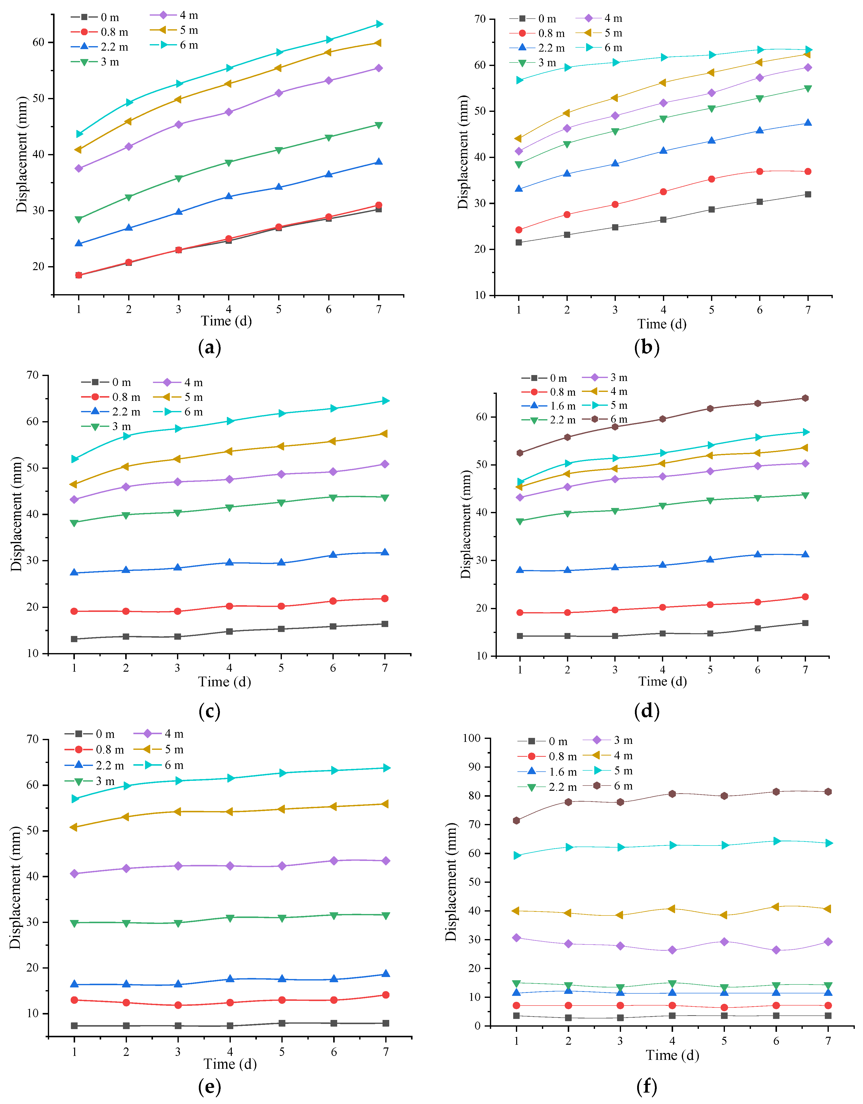
3.2. Different Rainfall Intensities

3.2.1. 200 mm/d

Stress nephogram, slope vector nephogram and displacement nephogram simulating the rainfall intensity of 200 mm/d are shown in Figure 5.

In an environment with a rainfall intensity of 200 mm/day, the slope experiences variations in stress, displacement, and strain vectors similar to those observed at 274 mm/day. Nonetheless, the 200 mm/day scenario results in marginally lower displacement and stress values. The stress cloud map (seen in Figure 5a) illustrates a reduction in the tensile stress areas in the first and second soil layers on the slope, along with a decrease in the maximum stress areas in the eighth and ninth layers at the base, where the peak stress is recorded at 33.859 kPa.

Upon analysis of the slope’s combined displacement chart (Figure 5b), this displacement lessens moving from the summit to base, with the lowest value at the slope’s foot. The contour map in Figure 5c reveals that the entire slip region forms a semi-circular arc with a diameter of 8.0 m, bisecting the slope’s base. Displacements within this arc consistently surpass 20 mm.

3.2.2. 300 mm/d

Figure 6 shows the change in cloud map at a rainfall intensity of 300 mm/d.

(1) Changes in Slope Stress:

In Figure 6a, the stress distribution map clearly shows that the first and second layers of soil on the incline are affected by tensile stress. This contrasts with the predominantly vertical stress observed on the slope itself. The area affected by tensile stress exceeds the extent seen in scenarios at the rainfall intensity of 274 mm/d. This implies a total slippage and failure in the soil of this particular area. Additionally, there is a noticeable escalation in stress beneath the second soil layer, peaking at the lower edge of the slope’s base. This peak stress reaches 52.151 kPa, signaling a substantial rise in the pressure exerted on the soil.

(2) Changes in Slope Displacement:

Figure 6b,c reveals significant insights into displacement variations. A notable increase in horizontal displacement is evident from the top towards the base of the slope, reaching the peak of 145.3 mm at the lower end. The zone impacted by this horizontal shift extends to about 4.0 m beneath the slope’s surface, with a pronounced change, over 40 mm, noticeable within the top 1.5 m layer. At the slope’s apex, the maximum vertical displacement recorded is 103.8 mm, which gradually lessens as one moves down to the base, where it measures 32 mm. The greatest displacements are predominantly observed, diminishing as one moves inward into the soil. In comparison to conditions at 274 mm/d of rainfall, the slip zone near the slope’s base extends roughly an additional 1.0 m downwards.

(3) Changes in Slope Strain Vector:

In Figure 6d, the direction of the strain vector is approximately perpendicular to the slope’s surface, while in other areas, the displacement vector is smaller with a direction roughly parallel to the Y direction. This indicates significant horizontal compression of the soil at the mentioned location, resulting in substantial displacement changes. The slope’s foot slides in the direction of this strain vector.

3.2.3. 400 mm/d

Figure 7 shows the stress and displacement cloud map at the 400 mm/d rainfall intensity.

In a scenario where the slope is subjected to a rainfall intensity of 400 mm/d, its response in terms of the stress, the displacement and the strain vector alterations shares notable similarities with a scenario of 300 mm/d rainfall intensity. However, in the case of the higher rainfall intensity, there is a pronounced increase in both stress and average displacement. As depicted in Figure 7a, the area experiencing the peak stress at the slope’s base expands in response to the escalating rainfall, culminating in a maximum stress of 51.856 kPa. In a similar vein, the greatest horizontal and cumulative displacements are observed at the slope’s base, reaching 178.6 mm and 189.8 mm (peak values).

Further analysis of Figure 7d reveals that the strain vector is most prominent at the slope’s base, peaking at 0.6372 mm. The intersection of soil layers 3 and 4 experiences the second highest strain, with its maximum value extending almost perpendicularly to the slope’s surface. This orientation suggests a sliding motion of the soil at the slope’s base in that direction. Meanwhile, strain vector variations in other areas of the slope are comparatively minor.

3.2.4. Comparative Analysis

(1) Slope displacement:

Figure 8 shows the displacement curves of the slope under different rainfall intensities. In order to study the movement patterns of slopes at different levels of rainfall, a number of noteworthy insights have emerged. With the increase in rainfall intensity, the slope displacement presents a more significant increment. It is worth noting that when the rainfall intensity is 400 mm/d, the maximum and minimum displacement of the slope’s foot reaches 189.8 mm. This indicates that higher rainfall intensity has a considerable influence on the horizontal displacement of the slope, leading to increased instability. Secondly, the maximum vertical displacement occurs at the slope crest. However, as rainfall intensity increases, the displacement difference between the top and bottom of the slope decreases after more than 300 mm/d. In fact, at a rainfall intensity of 200 mm/d, the displacement at the slope crest will be smaller than the displacement at the bottom. Once the rainfall intensity exceeds 274 mm/day. Under four simulated conditions, the maximum displacement of the slope’s foot is 26.34 mm, 81.4 mm, 134.9 mm and 180.85 mm, respectively. These findings suggest that as rainfall intensifies, it tends to soften and erode the soil at the foot of the slope, reducing its strength. As a result, soil decay intensifies, forcing accelerated soil displacement at the slope crest. Specifically, the combined displacement of the slope’s top and foot increased by 51.38 mm and 53.5 mm, respectively. On the other hand, the displacement changes were minimal in the rainfall intensity range of 250 mm/d to 274 mm/d. This means that when the rainfall intensity is lower than 300 mm/d, the slope will be significantly displaced and more prone to sliding and instability. Subsequently, after more than 300 mm/d, the increase in slope displacement becomes less pronounced, indicating that the effect of higher rainfall intensity on the slope is reduced.

(2) Comparative analysis

The displacement versus depth curves at measuring points 0~5 under simulated rainfall intensity of 200, 274, 300 and 400 mm/d are shown in Figure 9.

The following conclusions can be drawn:

(1) The horizontal displacement of the slope gradually decreases with an increase in depth. The displacement of soil above 3.0 m on the slope is larger, and that below 3.0 m is smaller. This indicates that slope soils are more likely to saturate and soften during rainfall, leading to a decrease in shear strength. Under the combined action of rainfall and self-weight, the slope slides easily. On the other hand, the soil on the underside is subjected to higher stress, resulting in greater deformation. However, the surrounding environment exerts significant constraints on soil deformation in this area, resulting in relatively small displacements.

(2) The slope moves downward from the foot, and the foot of the slope experiences both gravity and lateral anti-slip forces, resulting in large displacements. However, the displacement on the slope surface far from the foot gradually decreases, but its influence area is larger, leading to this pattern.

(3) Comparing the displacement changes at six measuring holes, the rainfall intensity has a significant impact on slope displacement. As rainfall intensity increases, the displacement at each measuring point also increases, with the maximum horizontal displacement occurring at a rainfall intensity of 400 mm/d. This suggests that this type of slope is most prone to sliding and instability when subjected to rainfall intensities within the range of 274–300 mm/d. It can be approximately considered that the maximum critical value of rainfall is 400 mm/d.

4. Conclusions

In this section, this research utilizes the ADINA finite element methodology to simulate and scrutinize slope deformation under varying rainfall intensities. The outcomes reveal insights into deformation spread, stress patterns, and additional relevant aspects, culminating in these key findings:

(1)

Correlation of simulated and actual slope displacements: There is a noteworthy alignment between the simulated and actual displacements of the slope. The internally simulated displacements, however, exhibit a marginal excess compared to the actual measurements.

(2)

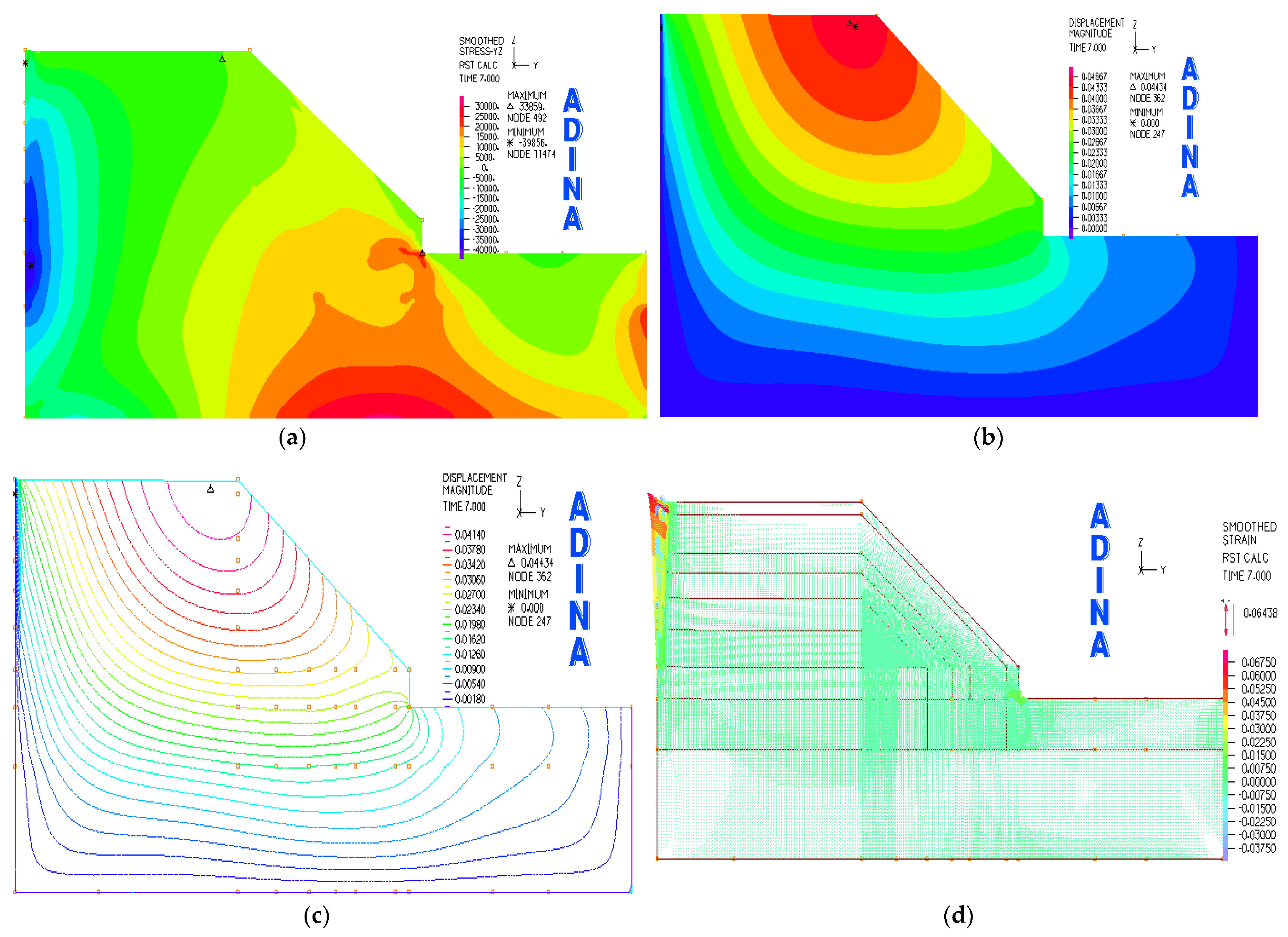
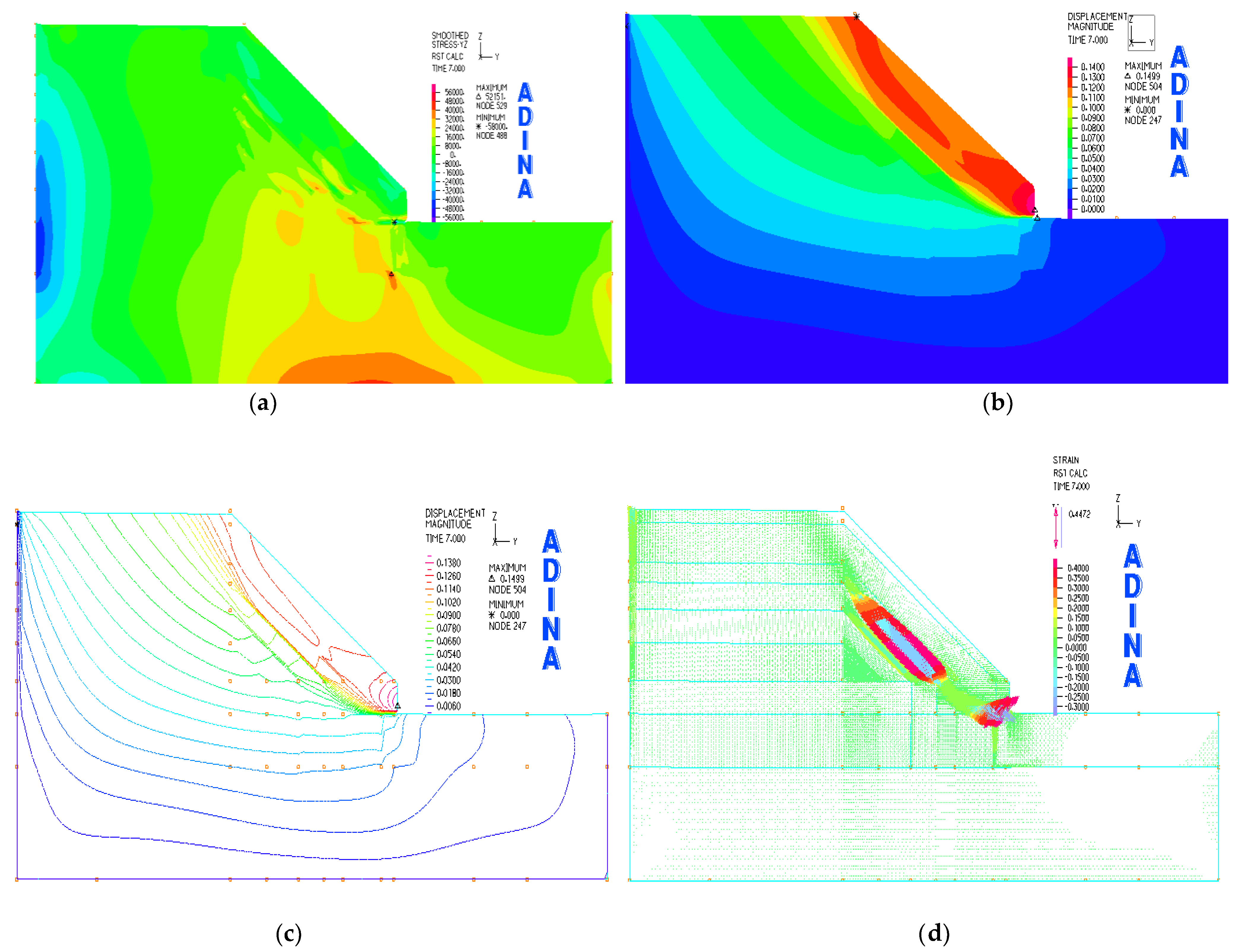
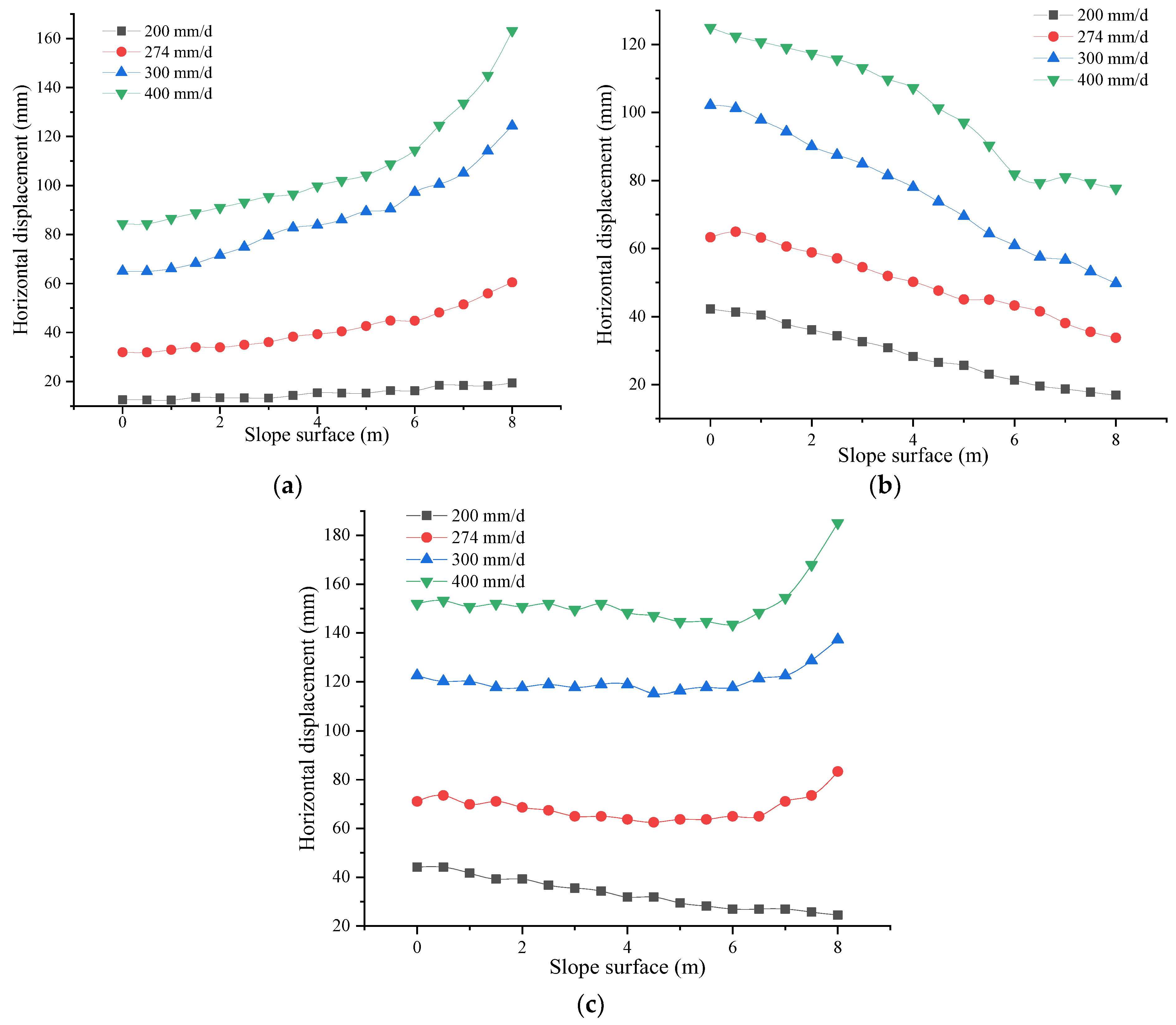
Rainfall intensity’s impact on slope deformation and stress: It is evident that the slope’s deformation and stress levels are sensitive to changes in rainfall intensity. An escalation in rainfall intensity correlates with increased deformation at the slope’s base and a broader area affected by stress. The peak in both displacement and stress is observed when rainfall intensity hits 400 mm/day. Slopes under rainfall intensities lower than 300 mm/day display a marked increase in deformation, heightening their susceptibility to slippage and instability. Conversely, intensities exceeding 300mm/day show a diminishing effect on slope deformation.

(3)

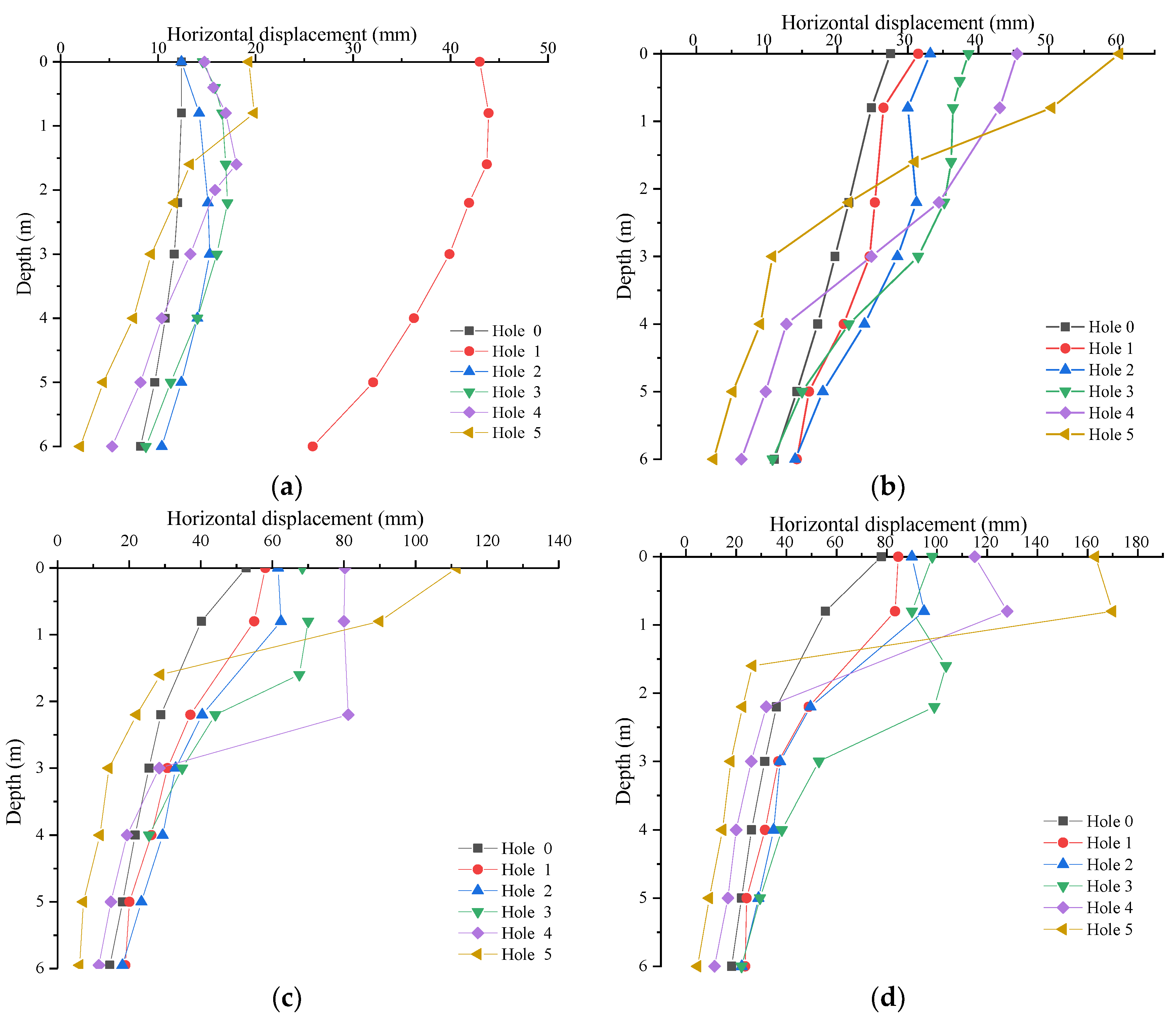
The rainfall intensity and its influence on displacement distribution: With the increase in rainfall intensity, soil horizontal displacement within 2.2 m of slope’s foot increases. In contrast, shallow soils 0.8 m above the surface showed relatively small shifts. Below 2.2 m, the horizontal displacement near the base decreases, and the displacement of the soil below 2.2 m is the least.

(4)

Sliding surfaces and their maximum expansion zones: Under a simulated rainfall intensity of 200 mm/day, the sliding surface manifests as a circular area at the base of the loess slope. However, at rainfall intensities of 274, 300 and 400 mm/day, the sliding surface shifts to a midpoint circular pattern. The maximal sliding zones are identified within arc distances of 1.0, 2.5, 3.5 and 4.0 m from the slope’s base, respectively.

References

1. Udvardi, B.; Kovács, I.J.; Szabó, C.; Falus, G.; Újvári, G.; Besnyi, A.; Bertalan, É.; Budai, F.; Horváth, Z. Origin and weathering of landslide material in a loess area: A geochemical study of the Kulcs landslide, Hungary. Environ. Earth Sci. 2016, 75, 1299. [Google Scholar] [CrossRef]
2. Wang, J.J.; Liang, Y.; Zhang, H.P.; Wu, Y.; Lin, X. A loess landslide induced by excavation and rainfall. Landslides 2014, 11, 141–152. [Google Scholar] [CrossRef]
3. Melillo, M.; Brunetti, M.T.; Peruccacci, S.; Gariano, S.L.; Guzzetti, F. An algorithm for the objective reconstruction of rainfall events responsible for landslides. Landslides 2015, 12, 311–320. [Google Scholar] [CrossRef]
4. Ering, P.; Babu, G.S. Characterization of critical rainfall for slopes prone to rainfall-induced landslides. Nat. Hazards Rev. 2020, 21, 06020003. [Google Scholar] [CrossRef]
5. Wang, G.; Li, T.; Xing, X.; Zou, Y. Research on loess flow-slides induced by rainfall in July 2013 in Yan’an, NW China. Environ. Earth Sci. 2015, 73, 7933–7944. [Google Scholar] [CrossRef]
6. Xu, L.; Qiao, X.; Wu, C.; Iqbal, J.; Dai, F. Causes of landslide recurrence in a loess platform with respect to hydrological processes. Nat. Hazards 2012, 64, 1657–1670. [Google Scholar] [CrossRef]
7. Chen, G.; Meng, X.; Qiao, L.; Zhang, Y.; Wang, S. Response of a loess landslide to rainfall: Observations from a field artificial rainfall experiment in Bailong River Basin, China. Landslides 2018, 15, 895–911. [Google Scholar] [CrossRef]
8. Huang, K.; Duan, H.; Yi, Y.; Yu, F.; Chen, S.; Dai, Z. Laboratory model tests on flow erosion failure mechanism of a slope consisting of anqing group clay gravel layer. Geofluids 2021, 2021, 1–14. [Google Scholar] [CrossRef]
9. Wang, F.; Xu, G.; Li, L.; Li, Z.; Li, P.; Zhang, J.; Cheng, Y. Response relationship between microtopographic variation and slope erosion under sand-cover. Water 2019, 11, 2488. [Google Scholar] [CrossRef]
10. Sun, D.; Wen, H.; Zhang, Y.; Xue, M. An optimal sample selection-based logistic regression model of slope physical resistance against rainfall-induced landslide. Nat. Hazards 2021, 105, 1255–1279. [Google Scholar] [CrossRef]
11. Morbidelli, R.; Saltalippi, C.; Flammini, A.; Govindaraju, R.S. Role of slope on infiltration: A review. J. Hydrol. 2018, 557, 878–886. [Google Scholar] [CrossRef]
12. Song, K.; Wang, F.; Liu, Y.; Huang, H. Landslide Deformation Prediction by Numerical Simulation in the Three Gorges, China. In Advancing Culture of Living with Landslides: Volume 5 Landslides in Different Environments; Springer International Publishing: Berlin/Heidelberg, Germany, 2017; pp. 309–315. [Google Scholar]
13. Uchida, T.; Nishiguchi, Y.; Matsumoto, N.; Sakurai, W. Observation and numerical simulation of debris flow induced by deep-seated rapid landslide. In Advancing Culture of Living with Landslides: Volume 4 Diversity of Landslide Forms; Springer International Publishing: Berlin/Heidelberg, Germany, 2017; pp. 399–405. [Google Scholar]
14. Arbanas, Ž.; Mihalić Arbanas, S.; Vivoda Prodan, M.; Peranić, J.; Sečanj, M.; Bernat Gazibara, S.; Krkač, M. Preliminary investigations and numerical simulations of a landslide reactivation. In Advancing Culture of Living with Landslides: Volume 2 Advances in Landslide Science; Springer International Publishing: Berlin/Heidelberg, Germany, 2017; pp. 649–657. [Google Scholar]
15. Mingtao, D.; Changfa, C.; Huazhong, Q. Accumulation landslide stability analysis based on FLAC numerical simulation. Disaster Adv. 2012, 5, 1783–1790. [Google Scholar]
16. Zhong, Q.M.; Chen, S.S.; Mei, S.A.; Cao, W. Numerical simulation of landslide dam breaching due to overtopping. Landslides 2018, 15, 1183–1192. [Google Scholar] [CrossRef]
17. Fan, Y.; Wu, F. A numerical model for landslide movement. Bull. Eng. Geol. Environ. 2022, 81, 105. [Google Scholar] [CrossRef]
18. Zerradi, Y.; Souissi, M.; Larabi, A. Application of the deterministic block theory to the slope stability design of an open-pit mine in Morocco. Min. Miner. Depos. 2023, 17, 53–60. [Google Scholar] [CrossRef]
19. Sdvyzhkova, O.; Moldabayev, S.; Başçetin, A.; Babets, D.; Kuldeyev, E.; Sultanbekova, Z.; Amankulov, M.; Issakov, B. Probabilistic assessment of slope stability at ore mining with steep layers in deep open pits. Min. Miner. Depos. 2022, 16, 11–18. [Google Scholar] [CrossRef]
20. Calista, M.; Pasculli, A.; Sciarra, N. Reconstruction of the geotechnical model considering random parameters distributions. In Engineering Geology for Society and Territory-Volume 2: Landslide Processes; Springer International Publishing: Berlin/Heidelberg, Germany, 2015; pp. 1347–1351. [Google Scholar]
21. Jeong, W.; Seong, J. Comparison of effects on technical variances of computational fluid dynamics (CFD) software based on finite element and finite volume methods. Int. J. Mech. Sci. 2014, 78, 19–26. [Google Scholar] [CrossRef]
22. Xi, R.; Xu, C.; Du, X.; El Naggar, M.H.; Wang, P.; Liu, L.; Zhai, E. Framework for dynamic response analysis of monopile supported offshore wind turbine excited by combined wind-wave-earthquake loading. Ocean Eng. 2022, 247, 110743. [Google Scholar] [CrossRef]
23. Mannacio, F.; Di Marzo, F.; Gaiotti, M.; Guzzo, M.; Rizzo, C.M.; Venturini, M. Characterization of underwater shock transient effects on naval E-glass biaxial fiberglass laminates: An experimental and numerical method. Appl. Ocean Res. 2022, 128, 103356. [Google Scholar] [CrossRef]
24. Tang, Y.; Lin, H.; Wang, Y.; Zhao, Y. Rock slope stability analysis considering the effect of locked section. Bull. Eng. Geol. Environ. 2021, 80, 7241–7251. [Google Scholar] [CrossRef]
25. Weng, X.; Sun, Y.; Yan, B.; Niu, H.; Lin, R.; Zhou, S. Centrifuge testing and numerical modeling of tunnel face stability considering longitudinal slope angle and steady state seepage in soft clay. Tunn. Undergr. Space Technol. 2020, 101, 103406. [Google Scholar] [CrossRef]
26. Huang, F.; Tao, S.; Chang, Z.; Huang, J.; Fan, X.; Jiang, S.H.; Li, W. Efficient and automatic extraction of slope units based on multi-scale segmentation method for landslide assessments. Landslides 2021, 18, 3715–3731. [Google Scholar] [CrossRef]
27. Li, Z.; Zhao, J.; Guan, C.; Liu, L.; Zhang, C. A field test study on the effect of artificial rainfall on instability characteristics of loess slopes. Arab. J. Geosci. 2023, 16, 400. [Google Scholar] [CrossRef]
Figure 1. Model grid division.
Water 16 00554 g001
Figure 2. Visualization of slope displacements under a rainfall intensity of 274 mm/day: (a) stress distribution in the Y-Z plane within the slope; (b) map showing horizontal shifts in the slope structure; (c) vertical movement visualization within the slope body; (d) overall displacement mapping of the entire slope; (e) detailed contour representation of slope movements; (f) diagram illustrating strain vectors across the slope.
Water 16 00554 g002
Figure 3. Horizontal displacement curve with slope distance.
Water 16 00554 g003
Figure 4. Displacement curves: (a) 0; (b) 1; (c) 2; (d) 3; (e) 4; (f) 5.
Water 16 00554 g004
Figure 5. Multi-faceted visualization of slope dynamics under 200 mm/day rainfall: (a) Y-Z axis stress distribution in slope structure; (b) overall slope body displacement graphic; (c) slope displacement variation contour illustration; (d) analytical strain vector mapping across the slopee.
Water 16 00554 g005
Figure 6. Multi-dimensional analysis of slope dynamics under 300 mm/d rainfall: (a) Y-Z axis stress visualization; (b) total displacement mapping; (c) displacement contour overview; (d) strain vector interpretation.
Water 16 00554 g006
Figure 7. Visualization of displacement patterns with a rainfall intensity at 300 mm/day: (a) stress distribution (Y-Z axis) in the slope; (b) comprehensive displacement overview of the slope; (c) detailed contour representation of slope movement; (d) diagram illustrating strain vectors in the slope.
Water 16 00554 g007
Figure 8. Displacement curve: (a) horizontal direction; (b) vertical direction; (c) total displacement.
Water 16 00554 g008
Figure 9. Variations in horizontal displacement at various depths: (a) 200 mm/day, (b) 274 mm/day, (c) 300 mm/day, (d) 400 mm/day.
Water 16 00554 g009
Disclaimer/Publisher’s Note: The statements, opinions and data contained in all publications are solely those of the individual author(s) and contributor(s) and not of MDPI and/or the editor(s). MDPI and/or the editor(s) disclaim responsibility for any injury to people or property resulting from any ideas, methods, instructions or products referred to in the content.