Discharge Formula and Hydraulics of Rectangular Side Weirs in the Small Channel and Field Inlet

Abstract

In this study, experimental investigations were conducted on rectangular side weirs with different widths and heights. Corresponding simulations were also performed to analyze hydraulic characteristics including the water surface profile, flow velocity, and pressure. The relationship between the discharge coefficient and the Froude number, as well as the ratios of the side weir height and width to upstream water depth, was determined. A discharge formula was derived based on a dimensional analysis. The results demonstrated good agreement between simulated and experimental data, indicating the reliability of numerical simulations using FLOW-3D software (version 11.1). Notably, significant fluctuations in water surface profiles near the side weir were observed compared to those along the center line or away from the side weir in the main channel, suggesting that the entrance effect of the side weir did not propagate towards the center line of the main channel. The proposed discharge formula exhibited relative errors within 10%, thereby satisfying the flow measurement requirements for small channels and field inlets.

1. Introduction

Sharp crested weirs are used to obtain discharge in open channels by solely measuring the water head upstream of the water. Side weirs, as a kind of sharp-crested weir, are extensively used for flow measurement, flow diversion, and flow regulation in open channels. Side weirs can be placed directly in the channel direction or field inlet, without changing the original structure of the channel. Thus, side weirs have certain advantages in the promotion and application of flow measurement facilities in small channels and field inlets. The rectangular sharp-crested weir is the most commonly available, and many scholars have conducted research on it.

Research on side weirs started in 1934. De Marchi studied the side weir in the rectangular channel and derived the theoretical formula based on the assumption that the specific energy of the main flow section of the rectangular channel in the side weir section was constant [1]. Ackers discussed the existing formulas for the prediction of the side weir discharge coefficient [2]. Chen concluded that the momentum theorem was more suitable for the analytical calculation of the side weir based on the experimental data [3]. Based on previous theoretical research, more and more scholars began to carry out experimental research on side weirs. Uyumaz and Muslu conducted experiments under subcritical and supercritical flow regimes and derived expressions for the side weir discharge and water surface profiles for these regimes by comparing them with experimental results [4]. Borghei et al. developed a discharge coefficient equation for rectangular side weirs in subcritical flow [5]. Ghodsian [6] and Durga and Pillai [7] developed a discharge coefficient equation of rectangular side weirs in supercritical flow. Mohamed proposed a new approach based on the video monitoring concept to measure the free surface of flow over rectangular side weirs [8]. Durga conducted experiments on rectangular side weirs of different lengths and sill heights and discussed the application of momentum and energy principles to the analysis of spatially varied flow under supercritical conditions. The results showed that the momentum principle was fitting better [7]. Omer et al. obtained sharp-crested rectangular side weirs discharge coefficients in the straight channel by using an artificial neural network model for a total of 843 experiments [9]. Emiroglu et al. studied water surface profile and surface velocity streamlines, and developed a discharge coefficient formula of the upstream Froude number, the ratios of weir length to channel width, weir length to flow depth, and weir height to flow depth [10]. Other investigators [11,12,13,14] have conducted experiments to study flow over rectangular side weirs in different flow conditions.

Numerous studies have been conducted in laboratories to this day. Compared to experimental methods, the numerical simulation method has many attractive advantages. We can easily obtain a wide range of hydraulic parameters of side weirs using numerical simulation methods, without investing a lot of manpower and resources. In addition, we can conduct small changes in inlet condition, outlet condition, and geometric parameters, and study their impact on the flow characteristics of side weirs. Therefore, with the development and improvement of computational fluid dynamics, the numerical simulation method has begun to be widely applied on side weirs. Salimi et al. studied the free surface changes and the velocity field along a side weir located on a circular channel in the supercritical regime by numerical simulation [15]. Samadi et al. conducted a three-dimensional simulation on rectangular sharp-crested weirs with side contraction and without side contraction and verified the accuracy of numerical simulation compared with the experimental results [16]. Aydin investigated the effect of the sill on rectangular side weir flow by using a three-dimensional computational fluid dynamics model [17]. Azimi et al. studied the discharge coefficient of rectangular side weirs on circular channels in a supercritical flow regime using numerical simulation and experiments [18]. The discharge coefficient over the two compound side weirs (Rectangular and Semi-Circle) was modeled by using the FLOW-3D software to describe the flow characteristics in subcritical flow conditions [19]. Safarzadeh and Noroozi compared the hydraulics and 3D flow features of the ordinary rectangular and trapezoidal plan view piano key weirs (PKWs) using two-phase RANS numerical simulations [20]. Tarek et al. investigated the discharge performance, flow characteristics, and energy dissipation over PK and TL weirs under free-flow conditions using the FLOW-3D software [21].

As evident from the aforementioned, the majority of studies have primarily focused on determining the discharge coefficient, while comparatively less attention has been devoted to investigating the hydraulic characteristics of rectangular side weirs. Numerical simulations were conducted on different types of side weirs, including compound side weirs and piano key weirs, in different cross-section channels under different flow regimes. It is imperative to derive the discharge formula and investigate other crucial flow parameters such as depth, velocity, and pressure near side weirs for their effective implementation in water measurement. In this study, a combination of experimental and numerical simulation methods was employed to examine the relationship between the discharge coefficient and its influencing factors; furthermore, a dimensionless analysis was utilized to derive the discharge formula. Additionally, water surface profiles near side weirs and pressure distribution at the bottom of the side channel were analyzed to assess safety operation issues associated with installing side weirs.

2. Principle of Flow Measurement

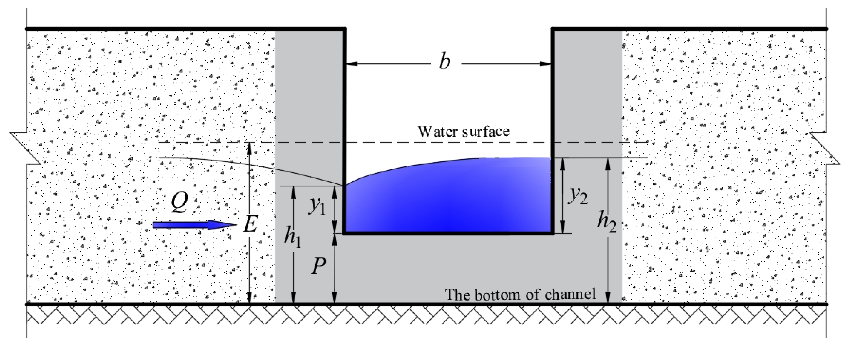
Flow discharge over side weirs is a function of different dominant physical and geometrical quantities, which is defined as

$$Q=f(b,B,P,v,h_1,g,\mu ,\sigma ,\rho ,i),$$

(1)

where Q is flow discharge over the side weir, b is the side weir width, B is the channel width, P is the side weir height, v is the mean velocity, h₁ is water depth upstream the side weir in the main channel, g is the gravitational acceleration, μ is the dynamic viscosity of fluid, ρ is fluid density, and i is the channel slope (Figure 1).

In experiments when the upstream weir head was over 30 mm, the effects of surface tension on discharge were found to be minor [22]. The viscosity effect was far less than the gravity effect in a turbulent flow. Hence μ and σ were excluded from the analysis [23,24]. In addition, the channel width, the channel slope, and the fluid density were all constant, so the discharge formula can be simplified as:

$$Q=f_1(b,P,v,h_1,g),$$

(2)

According to the Buckingham π theorem, the following relationship among the dimensionless parameters is established:

$$f_2(Q,b,P,v,h_1,g)=0,$$

(3)

Selected h₁ and g as basic fundamental quantities, and the remaining physical quantities were represented in terms of these fundamental quantities as follows:

$$F({\pi }_1,{\pi }_2,{\pi }_3,{\pi }_4)=0,$$

(4)

In which

$${\pi }_1=\frac{Q}{h_1^{r_{11}}{g}^{r_{12}}},{\pi }_2=\frac{b}{h_1^{r_{21}}{g}^{r_{22}}},{\pi }_3=\frac{P}{h_1^{r_{31}}{g}^{r_{32}}},{\pi }_4=\frac{v}{h_1^{r_{41}}{g}^{r_{42}}}$$

Based on dimensional analysis, the following equations were derived.

$$r_{11}=2.5,r_{12}=0.5,r_{21}=1,r_{22}=0,r_{31}=1,r_{32}=0,r_{41}=0.5,r_{42}=0.5,$$

Namely

$$F(\frac{Q}{h_1^2\sqrt{g{h}_1}},\frac{b}{h_1},\frac{P}{h_1},\frac{v}{\sqrt{g{h}_1}})=0$$

(5)

So the discharge formula can be simplified as:

$$Q=\frac{h_1}{\sqrt{2}b}{F}_1(\frac{b}{h_1},\frac{P}{h_1},\frac{v}{\sqrt{g{h}_1}})b\sqrt{2g}{h}_1^{1.5},$$

(6)

In a sharp-crested weir, discharge over the weir is proportional to $H_1^{1.5}$ (H₁ is the upstream total head above the crest, namely H₁ = y₁ + v²/2 g), so Equation (6) can be transformed as follows:

$$Q=\frac{h_1}{\sqrt{2}b}{F}_1(\frac{b}{h_1},\frac{P}{h_1},\frac{v}{\sqrt{g{h}_1}})b\sqrt{2g}{H}_1^{1.5},$$

(7)

Consequently, the discharge formula over rectangular side weirs is defined as follows, in which $m=f(\frac{b}{h_1}$,$\frac{P}{h_1},F{r}_1)$. Parameter m represents the dimensionless discharge coefficient. Parameter Fr₁ represents the Froude number at the upstream end of the side weir in the main channel.

$$Q=\frac{2}{3}mb\sqrt{2g}{H}_1^{1.5},$$

(8)

3. Experiment Setup

The experimental setup contained a storage reservoir, a pumping station, an electromagnetic flow meter, a control valve, a stabilization pond, rectangular channels, a side weir, and a sluice gate. The layout of the experimental setup is shown in Figure 2. Water was supplied from the storage reservoir using a pump. The flow discharge was measured with an electromagnetic flow meter with precision of ±3‰. Water depth was measured with a point gauge with an accuracy of ±0.1 mm. The flow velocity was measured with a 3D Acoustic Doppler Velocimeter (Nortek Vectrino, manufactured by Nortek AS in Rud, Norway). In order to eliminate accidental and human error, multiple measurements of the water depth and flow velocity at the same point were performed and the average values were used as the actual water depth and flow velocity of the point. The main and side channels were both rectangular open channels measuring 47 cm in width and 60 cm in height. The geometrical parameters of rectangular side weirs are shown in

Table 1. The geometrical parameters of rectangular side weirs.

B/cm	P/cm	b/cm	B/cm	P/cm	b/cm
47	7	47	47	15	47
		40			40
		30			30
		20			20
47	10	47	47	20	47
		40			40
		30			30
		20			20

.

When water passes through a side weir, its quality point is affected not only by gravity but also by centrifugal inertia force, leading to an inclined water surface within that particular cross-section before reaching the weir. In order to examine water profiles adjacent to side weirs, cross-sectional measurements were conducted at regular intervals of 12 cm both upstream and downstream of each side weir, denoted as sections ① to ⑩, respectively. Measuring points were positioned near the side weir (referred to as “Side I”), along the center line of the main channel (referred to as “Side II”), and far away from the side weir (referred to as “Side III”) for each cross-section. The schematic diagram illustrating these measuring points is presented in Figure 3.

4. Numerical Simulation Settings

4.1. Mathematical Model

4.1.1. Governing Equations

Establishing the controlling equations is a prerequisite for solving any problem. For the flow analysis problem of water flowing over a side weir in a rectangular channel, assuming that no heat exchange occurs, the continuity equation (Equation (9)) and momentum equation (Equation (10)) can be used as the controlling equations as follows:

The continuity equation:

$$\frac{\partial \rho }{\partial t}+\frac{\partial \left(\rho u_i\right)}{\partial x_i}=0,$$

(9)

Momentum equation:

$$\frac{\partial \left(\rho u_i\right)}{\partial t}+\frac{\partial \left(\rho u_i{u}_j\right)}{\partial x_j}=\frac{\partial }{\partial x_j}\left(\mu \frac{\partial u_i}{\partial x_j}\right)-\frac{\partial p}{\partial x_i}+S_i,$$

(10)

where: ρ is the fluid density, kg/m³; t is time, s; u_i, u_j are average flow velocities, u₁, u₂, u₃ represent average flow velocity components in Cartesian coordinates x, y, and z, respectively, m/s; μ is dynamic viscosity of fluid, N·s/m²; p is the pressure, pa; S_i is the body force, S₁ = 0, S₂ = 0, S₃ = −ρg, N [24].

4.1.2. RNG k-ε Model

The water flow in the main channel is subcritical flow. When the water flows through the side weir, the flow line deviates sharply, the cross section suddenly decreases, and due to the blocking effect of the side weir, the water reflects and diffracts, resulting in strong changes in the water surface and obvious three-dimensional characteristics of the water flow [25]. Therefore the RNG k-ε model is selected. The model can better handle flows with greater streamline curvature, and its corresponding k and ε equation is, respectively, as follows:

$$\frac{\partial \left(\rho k\right)}{\partial t}+\frac{\partial \left(\rho k{u}_i\right)}{\partial x_i}=\frac{\partial }{\partial x_j}\left[{\alpha }_k{\mu }_{\mathrm{eff}}\frac{\partial k}{\partial x_j}\right]+G_k+\rho \epsilon ,$$

(11)

$$\frac{\partial \left(\rho \epsilon \right)}{\partial t}+\frac{\partial \left(\rho \epsilon u_i\right)}{\partial x_i}=\frac{\partial }{\partial x_j}\left[{\alpha }_k{\mu }_{eff}\frac{\partial \epsilon }{\partial x_j}\right]+\frac{C_{1\epsilon }^{*}\epsilon }{k}{G}_k-C_{2\epsilon }\rho \frac{{\epsilon }^2}{k}$$

(12)

where: k is the turbulent kinetic energy, m²/s²; μ_eff is the effective hydrodynamic viscous coefficient; G_k is the generation item of turbulent kinetic energy k due to gradient of the average flow velocity; ${\mathrm{C}}_{1\mathsf{\epsilon }}^{*}$, C_2ε are empirical constants of 1.42 and 1.68, respectively; ε is turbulence dissipation rate, kg·m²/s².

4.1.3. TruVOF Model

Because the shape of the free surface is very complex and the overall position is constantly changing, the fluid flow phenomenon with a free surface is a typical flow phenomenon that is difficult to simulate. The current methods used to simulate free surfaces mainly include elevation function method, the MAC method [26] and the VOF (Volume of Fluid) method [27]. The VOF method is a method proposed by Hirt and Nichols to deal with the complex motion of the free surface of a fluid, which can describe all the complexities of the free surface with only one function. The basic idea of the method is to define functions α_w and α_a, which represent the volume percentage of the calculation area occupied by water and air, respectively. In each unit cell, the sum of the volume fractions of water and air is equal to 1, i.e.,

$${\alpha }_{\mathrm{w}}+{\alpha }_{\mathrm{a}}=1$$

(13)

The TruVOF calculation method can accurately track the change of free liquid level and accurately simulate the flow problems with free interface. Its equation is:

$$\frac{\partial F}{\partial t}+{\underset{\_}{\overline{u}}}_m\cdot \nabla F=0,$$

(14)

where: ${\overline{\underset{\_}{u}}}_m$ is the average velocity of the mixture; t is the time; F is the volume fraction of the required fluid.

4.2. Parameter Setting and Boundary Conditions

To streamline the iterative calculation and minimize simulation time, we selected a main channel measuring 7.5 m in length and a side channel measuring 2.5 m in length for simulation. Three-dimensional geometrical models were developed using the software AutoCAD (version 2016-Simplified Chinese). The spatial domain was meshed using a constructed rectangular hexahedral mesh and each cell size was 2 cm. A volume flow rate was set in the channel inlet with an auto-adjusted fluid height. An outflow–outlet condition was positioned at the end of the side channel. A symmetry boundary condition was set in the air inlet at the top of the model, which represented that no fluid flows through the boundary. The lower Z (Zmin) and both of the side boundaries were treated as a rigid wall (W). No-slip conditions were applied at the wall boundaries. Figure 4 illustrates these boundary conditions.

5. Results

5.1. Water Surface Profiles

Water surface profiles were crucial parameters for selecting water-measuring devices. Upon analyzing the consistent patterns observed in different conditions, one specific condition was chosen for further analysis. To validate the reliability of numerical simulation, measured and simulated water depths of rectangular side weirs with different widths and heights at a discharge rate of 25 L/s were extracted for comparison (

Table 2. Comparison of measured and simulated water depths on Side I of each side weir at a discharge of 25 L/s.

P/cm	Section Position	b = 20 cm			b = 30 cm			b = 40 cm			b = 47 cm
		hm/cm	hs/cm	R/%	hm/cm	hs/cm	R/%	hm/cm	hs/cm	R/%	hm/cm	hs/cm	R/%
7	④	21.49	19.4	9.73	17.74	16.9	4.74	16.07	14.51	9.71	13.79	12.50	9.35
	④′	20.48	19.05	6.98	17.78	16.14	9.22	15.69	14.31	8.80
	⑥	20.71	19.02	8.16	17.82	16.31	8.47	15.92	14.53	8.73	15.23	13.80	9.39
	⑧′	22.00	20.22	8.09	18.27	16.74	8.37	16.59	14.96	9.83
	⑧	22.37	20.17	9.83	17.73	16.80	5.25	16.27	15.08	7.31	15.36	14.36	6.51
10	④	24.15	22.6	6.42	19.96	18.84	5.61	19.03	18.58	2.36	16.83	15.85	5.82
	④′	24.21	22.05	8.92	19.49	18.19	6.67	18.75	18.35	2.13
	⑥	24.01	21.78	9.29	19.65	18.34	6.67	18.95	18.63	1.69	17.52	16.09	8.16
	⑧′	24.88	22.4	9.97	20.65	19.21	6.97	20.12	19.29	4.13
	⑧	24.03	22.96	4.45	21.16	19.34	8.60	19.71	19.43	1.42	18.39	17.36	5.60
15	④	28.85	27.56	4.47	25.86	24.09	6.84	24.05	21.89	8.98	22.73	20.80	8.49
	④′	28.49	26.97	5.34	25.19	23.84	5.36	23.42	21.46	8.37
	⑥	28.85	26.98	6.48	25.72	23.99	6.73	23.23	21.82	6.07	23.10	21.05	8.87
	⑧′	28.96	27.30	5.73	26.38	24.19	8.30	24.18	22.27	7.90
	⑧	29.18	27.96	4.18	26.57	24.54	7.64	24.57	22.33	9.12	23.20	21.10	9.05
20	④	33.29	32.34	2.85	30.63	29.02	5.26	28.49	26.87	5.69	26.99	25.81	4.37
	④′	33.14	31.95	3.59	29.75	28.62	3.80	28.11	26.79	4.70
	⑥	33.32	31.79	4.59	30.04	28.45	5.29	28.99	26.86	7.35	27.42	26.72	2.55
	⑧′	34.02	32.39	4.79	30.69	28.95	5.67	29.59	27.25	7.91
	⑧	34.62	32.84	5.14	31.44	29.29	6.84	29.51	27.31	7.46	28.21	27.00	4.29

Note: h_m represents the measured water depth, h_s represents the simulated water depth, R represents the absolute relative error, ④′ represents the section at the upstream end of the weir crest, ⑧′ represents the section at the downstream end of the weir crest, the same below.

and Figure 5). The results in Table 2 and Figure 5 indicate a maximum absolute relative error value of 9.97% and all absolute relative error values within 10%, demonstrating satisfactory agreement between experimental and simulated results.

Due to the diversion caused by the side weir, there was a rapid variation in flow near the side weir in the main channel. In order to investigate the impact of the side weir on water flow in the main channel, water surface profiles on Side I, Side II, and Side III were plotted with a side weir width and height both set at 20 cm at a discharge rate of 25 L/s (Figure 6). As depicted in Figure 6, within a certain range of the upstream end of the main channel, water depths on Side I, Side II, and Side III were nearly equal with almost horizontal profiles. As the distance between the location of water flow and the upstream end of the weir crest decreased gradually, there was a gradual decrease in water depth on Side I along with an inclined trend in its corresponding profile; however, both Side II and Side III still maintained almost horizontal profiles. When approaching closer to the side weir area with flowing water, there was an evident reduction in water depth on Side I accompanied by a significant downward trend visible across an expanded decline range. The minimum point occurred near the upstream end of the weir crest before gradually increasing again towards downstream sections. At the crest section of the side weir, there is an upward trend observed in the water surface. The water surface tended to stabilize downstream of the main channel within a certain range from the downstream end of the weir crest. There was no significant change in the water surface profiles of Side Ⅱ and Side Ⅲ in the crest section. It can be inferred that the side weir entrance effect occurred only between Side Ⅰ and Side Ⅱ. M. Emin reported the same pattern [10].

For a more accurate study on the entrance effect of the side weir on the Water Surface Profile (WSP) for Side I; a comparative analysis conducted using different widths but the same height (15 cm) at a discharge rate of 25 L/s is presented through Figure 7, Figure 8, Figure 9 and Figure 10.

According to Figure 7, Figure 8, Figure 9 and Figure 10, the water depth upstream of the main channel started to decrease as it approached the upstream end of the weir crest and then gradually increased at the weir crest section. In other words, the water surface profile exhibited a backwater curve along the length of the weir crest. The water depth remained relatively stable downstream of the main channel within a certain range from the downstream end of the weir crest. Additionally, there was a higher water depth downstream of the main channel compared to that upstream of the main channel. Furthermore, an increase in the width of the side weir led to a gradual reduction in fluctuations on its water surface.

5.2. Velocity Distribution

The law of flow velocity distribution near the side weir is the focus of research and analysis, so the simulated and measured values of flow velocity near the side weir were compared and analyzed. Take the discharge of 25 L/s, the height of 15 cm, and the width of 30 cm of the side weir as an example to illustrate. Figure 11 shows the measured and simulated velocity distribution in the x-direction of cross-section ④. As can be seen from Figure 11, the diagrams of the measured and simulated velocity distribution were relatively consistent, and the maximum absolute relative error between the measured and simulated values at the same measurement point was 9.37%, and the average absolute relative error was 3.97%, which indicated a satisfactory agreement between the experimental and simulated results.

From Figure 11, it can be seen that the flow velocity gradually increased from the bottom of the channel towards the water surface in the Z-direction, and the flow velocity gradually increased from Side Ⅲ to Side Ⅰ in the Y-direction. The maximum flow velocity occurred near the weir crest.

Figure 12 shows the distribution of flow velocity at different depths (z/P = 0.3, z/P = 0.8, z/P = 1.6) with a side weir width of 30 cm and height of 15 cm at a discharge of 25 L/s. The water flow line began to bend at a certain point upstream of the main channel, and the closer it was to the upstream end of the weir crest, the greater the curvature. The maximum curvature occurred at the downstream end of the weir crest. The flow patterns at the bottom, near the side weir crest, and above the side weir crest were significantly different. There was a reverse flow at the bottom of the main channel, where the forward and reverse flows intersect, resulting in a detention zone. The maximum flow velocity at the bottom layer occurred at the upstream end of the side weir crest. When the location of water flow approached the weir crest, the maximum flow velocity occurred at the upstream end of the weir crest. The maximum flow velocity on the water surface occurred at the downstream end of the weir crest. As the water depth decreased, the position of the maximum flow velocity gradually moved from the upstream end of the side weir to the downstream end of the side weir.

5.3. Side Channel Pressure Distribution

When water flowed through the side weir, an upstream water level was formed, resulting in a pressure zone at the junction with the side channel. This pressure zone led to increased water pressure on the floor of the side channel, which affected its stability and durability. In small channels or fields where erosion resistance is weak, excessive pressure can cause scour holes. Therefore, analyzing the pressure distribution in the side channel is necessary to select an appropriate height and width for the side weir that effectively reduces its impact on the bottom plate.

To investigate the impact of side weir width on hydraulic characteristics, pressure data was collected at a discharge rate of 25 L/s for side weirs with heights of 20 cm and widths ranging from 20 cm to 47 cm. The pressure distribution map was drawn, as shown in Figure 13.

As can be seen from Figure 13, the pressure at the bottom of the side channel decreased as the width of the side weir increased. This uneven distribution of water flow on the weir was caused by the sharp bending of water flow lines and the influence of centrifugal inertia force over a short period. After passing through the side weir, the water flow became symmetrically distributed with respect to the axis of the side channel, leaning towards the right bank at a certain distance. As we increased the width of the side weir, we noticed that its position gradually approached the side weir and maximum pressure decreased at this location where the water tongue formed due to flowing through it (Figure 13). For a constant height (20 cm) but varying widths (20 cm, 30 cm, 40 cm, and 47 cm), we measured maximum pressures at these positions as follows: 103,713 Pa, 103,558 Pa, 103,324 Pa, and 103,280 Pa, respectively. Consequently, increasing width reduced the impact on the side channel from water flowing through it while changing pressure distribution from concentration to dispersion in a vertical direction. In the practical application of side weirs, appropriate height should be selected based on the bottom plate’s capacity to withstand the pressure exerted by flowing water within channels.

To investigate how height affects the hydraulic characteristics of rectangular side weirs further (Figure 14), we extracted pressures on bottom plates when discharge was fixed at 25 L/s while varying heights were set as follows: 7 cm, 10 cm, 15 cm, and 20 cm, respectively.

As shown in Figure 14, when the width of the side weir was constant, the pressure at the bottom of the side channel increased with the height of the side weir. As the height of the side weir increased, the water tongue formed by flow through the side weir gradually moved away from it in a downstream direction. In terms of vertical water flow, as the height of the side weir increased, the position of maximum pressure at which the water tongue falls shifted closer to the axis of the side channel from its right bank. Moreover, an increase in height resulted in higher maximum pressure at this falling point. For a constant width (20 cm) and varying heights (7 cm, 10 cm, 15 cm, and 20 cm), corresponding maximum pressures at this landing point were measured as 102,422 Pa, 102,700 Pa, 103,375 Pa, and 103,766 Pa, respectively. Consequently, increasing width led to a greater impact on both flow through and pressure distribution within the side channel; transforming it from scattered to concentrated along its lengthwise direction. Therefore, when applying such weirs practically one should select an appropriate width based on what pressure can be sustained by their respective channel bottom plates.

5.4. Discharge Coefficient

Based on dimensionless analysis, the influencing parameters of the discharge coefficient were obtained. To study the effect of parameters Fr₁, b/h₁, and P/h₁, discharge coefficient values were plotted against Fr₁, b/h₁, and P/h₁, shown in Figure 15, Figure 16 and Figure 17. The discharge coefficient decreased as parameters Fr₁ and b/h₁ increased. The discharge coefficient increased as parameter P/h₁ increased. As Uyumaz and Muslu reported in a previous study, the variation of the discharge coefficient with respect to the Froude number showed a second-degree curve for a subcritical regime [4].

Quantitative analysis between discharge coefficient values and parameters Fr₁, b/h_1, and P/h₁ was conducted using data analysis software (IBM SPSS Statistics 19). The various coefficients obtained are shown in

Table 3. Coefficient.

Model	Unstandardized Coefficients		Standardized Coefficients	t	Sig
	B	Std. Error	Beta (β)
Constant	−1.294	0.155		−8.369	0.000
Fr1	3.430	0.286	3.401	12.013	0.000
b/h1	−0.004	0.004	−0.045	−0.944	0.348
P/h1	2.401	0.167	4.064	14.394	0.000

.

The value of t and Sig are the significance results of the independent variable, and the value of Sig corresponding to the value of t is less than 0.05, indicating that the independent variable has a significant impact on the dependent variable. Therefore, the values of Sig corresponding to the parameters Fr₁ and P/h₁ were less than 0.05, indicating that the parameters Fr₁ and P/h₁ have a significant impact on the discharge coefficient. On the contrary, the parameter b/h₁ has less impact on the discharge coefficient. Therefore, quantitative analysis between discharge coefficient values and parameters Fr₁, and P/h₁ was conducted using data analysis software by removing factor b/h₁. The model summary, ANOVA, and coefficient obtained are shown respectively in

Table 4. Model Summary ^b.

Model	R	R Square	Adjusted R Square	Std. Error of the Estimate
1	0.913 a	0.833	0.829	0.03232

Note: ^a. Predictors:(Constant), Fr₁, P/h₁; ^b. Discharge coefficient.

,

Table 5. ANOVA ^b.

Model		Sum of Squares	df	Mean Square	F	Sig
1	Regression	0.402	2	0.201	192.545	0.000 a
	Residual	0.080	77	0.001
	Total	0.483	79

Note: ^a. Predictors:(Constant), Fr₁, P/h₁; ^b. Discharge coefficient.

and

Table 6. Coefficient ^a.

Model	Unstandardized Coefficients		Standardized Coefficients	t	Sig
	B	Std. Error	Beta (β)
Constant	−1.326	0.151		−8.796	0.000
Fr1	3.479	0.281	3.449	12.396	0.000
P/h1	2.427	0.164	4.108	14.765	0.000

Note: ^a. Predictors:(Constant), Fr₁, P/h₁.

. R and adjusted R square in Table 4 were approaching 1, which indicated the goodness of fit of the regression model was high. The value of Sig corresponding to the value of F in Table 5 was less than 0.05, which indicated that the regression equation was useful. The values of Sig corresponding to the parameters Fr₁ and P/h₁ in Table 6 were less than 0.05, indicating that the parameters Fr₁ and P/h₁ have a significant impact on the discharge coefficient.

Based on the above analysis, the flow coefficient formula has been obtained, shown as follows:

$$m=3.479F{r}_1+2.427(\frac{P}{h_1}) - 1.326, {\mathrm{R}}^2 = 0.829$$

(15)

Discharge formula were obtained by substituting Equation (15) into Equation (12), as shown in Equation (16).

$$Q=[3.479F{r}_1+2.427(\frac{P}{h_1})-1.326]b\sqrt{2g}{H}_1^{1.5}, {\mathrm{R}}^2 = 0.829$$

(16)

where Q ∈ [0.006, 0.030], m³/s; b ∈ [0.20, 0.47], m; P ∈ [0.07, 0.20], m.

Figure 18 showed the measured discharge coefficient values with those calculated from discharge formulas in Table 3. The scatter of the data with respect to perfect line was limited to ±10%.

6. Discussions

Determining water surface profile near the side weir in the main channel is one of the tasks of hydraulic calculation for side weirs. As the water flows through the side weir, discharge in the main channel is gradually decreasing, namely $\frac{dQ}{ds}<0$. According to the Equation (17) derived from Qimo Chen [3], it can be inferred that the value of $\frac{dh}{ds}$ is greater than zero in subcritical flow (Fr < 1), that is, the water surface profile near the side weir in the main channel is a backwater curve. Due to the side weir entrance effect at the upstream end, water surface profiles drop slightly at the upstream end of the side weir crest, as EI-Khashab [28] and Emiroglu et al. [29] reported in previous experimental studies.

$$\frac{dh}{ds}=\frac{-K\frac{Q}{g\omega }\frac{dQ}{ds}}{1-F{r}^2}$$

(17)

In this study, the water surface profile exhibited a backwater curve along the length of the weir crest. Therefore, during side weir application, it is crucial to ensure that downstream water levels do not exceed the highest water level of the channel.

The head on the weir is one of the important factors that flow over side weirs depends on. At the same time, the head depends on the water surface profile near the side weir in the main channel. Therefore, further research on the quantitative analysis of water surface profile needs to be conducted. Mohamed Khorchani proposed a new approach based on the video monitoring concept to measure the free surface of flow over side weirs. It points out a new direction for future research [8].

The maximum flow velocity, a key parameter in assessing the efficiency of a weir, occurs at the upstream end of the weir crest, typically near the crest. This is attributed to the convergence of the flow as it approaches the crest, resulting in a significant increase in velocity. It was found that in this study the minimum flow velocity occurred at the bottom of the main channel away from the side weir. Under such conditions, the accumulation of sediments could lead to siltation, which in turn can affect the accuracy of flow measurement through side weirs. This is because the presence of sediments can alter the flow patterns and cause errors in the measurement. Therefore, it becomes crucial to explore methods to optimize the selection of side weirs in order to minimize or eliminate the effects of sedimentation on flow measurement.

Pressure distribution plays a crucial role in ensuring structural safety for side weirs since small channels and field inlets have relatively limited pressure-bearing capacities. Therefore, it is important to select an appropriate geometrical parameter of rectangular side weirs based on their ability to withstand the pressure exerted on their bottom combined with pressure distribution data at the bottom of the side channel we have obtained in this study.

The discharge coefficient formula (Equation (15)), which incorporates Fr₁ and P/h₁, was derived based on dimensional analysis. However, it is worth noting that previous research has contradicted this formula by suggesting that the discharge coefficient solely depends on the Froude number. This conclusion can be observed in this study such as in Equations (18)–(23) in

Table 7. Discharge coefficient formulas of rectangular side weirs presented in previous studies.

Discharge Coefficient Formulas	Researchers	Number of Formula
$m=0.864{\left(\frac{1-F{r}_1^2}{2+F{r}_1^2}\right)}^{0.5}$	Subramanya and Awasthy [30]	(18)
$m=0.432{\left(\frac{2-F{r}_1^2}{1+2F{r}_1^2}\right)}^{0.5}$	Nandesamoorthy et al. [31]	(19)
$m=0.623-0.222F{r}_1$	Yu-Tech [32]	(20)
$m=0.81-0.6F{r}_1$	Ranga Raju et al. [33]	(21)
$m=0.485{\left(\frac{2+F{r}_1^2}{2+3F{r}_1^2}\right)}^{0.5}$	Hager [34]	(22)
$m=0.45-0.221F{r}_1^2$	Cheong [35]	(23)
$m=0.33-0.18F{r}_1+0.49\left(\frac{P}{h_1}\right)$	Singh et al. [37]	(24)
$m=1.06{\left[{\left(\frac{14.14P}{8.15P+h_1}\right)}^{10}+{\left(\frac{h_1}{h_1+P}\right)}^{15}\right]}^{-0.1}$	Swamee et al. [36]	(25)
$m=0.71-0.41F{r}_1-0.22\left(\frac{P}{h_1}\right)$	Jalili et al. [38]	(26)
$m=0.7-0.48F{r}_1-0.3\left(\frac{P}{h_1}\right)+0.06\frac{b}{B}$	Borghei et al. [5]	(27)
$m=0.9236-0.3247F{r}_1-0.0521F{r}_1^2$	Durga and Pillai [7]	(28)
$m={\left[0.836+{\left(-0.035+0.39{\left(\frac{P}{h_1}\right)}^{12.69}+0.158{\left(\frac{b}{B}\right)}^{0.59}+0.049{\left(\frac{b}{h_1}\right)}^{0.42}+0.244F{r}_1^{2.215}\right)}^{3.018}\right]}^{5.36}$	M.E. Emiroglu et al. [10]	(29)

of the manuscript [30,31,32,33,34,35], which clearly demonstrate the dependency of the discharge coefficient on the Froude number. In contrast, our derived discharge coefficient formula (Equation (15)) offers a more streamlined and simplified approach compared to Equation (25) [36] and Equation (29) [10]—making it easier to comprehend and apply—an advantageous feature particularly valuable in fluid dynamics where intricate calculations can be time-consuming. Furthermore, our derived discharge coefficient formula (Equation (15)) exhibits a broader application scope than that of Equation (24) [37] as shown in

Table 8. Application scope of discharge coefficient formulas.

Discharge/(L·s−1)	Width of Side Weir/cm	Height of Side Weir/cm	Number of Formula
10~14	10~20	6~12	(24)
35–100	20~75	1~19	(26), (27)
6~30	20~47	7~20	(15)

. Equation (26) [38] and Equation (27) [5] are specifically applicable under high flow discharge conditions. Conversely, our derived discharge coefficient formula (Equation (15)) is better suited for low-flow discharge conditions.

In addition to the factors studied in the paper, factors such as the sediment content in the flow, the bottom slope, and the cross-section shape of the channel also have a certain impact on the hydraulic characteristics of the side weir. Further numerical simulation methods can be used to study the hydraulic characteristics and the influencing factors of the side weir. Water measurement facilities generally require high accuracy of water measurement, the flow of sharp-crested side weirs is complex, and the water surface fluctuates greatly. While conducting numerical simulations, experimental research on prototype channels is necessary to ensure the reliability of the results and provide reference for the body design and optimization of side weirs in small channels and field inlets.

7. Conclusions

This paper presents a comprehensive study that encompasses both experimental and numerical simulation research on rectangular side weirs of varying heights and widths within rectangular channels. A thorough analysis of the experimental and numerical simulation results has been conducted, leading to the derivation of several notable conclusions:

(1)

A comparative analysis was conducted on the measured and simulated values of water depth and flow velocity. Both of the maximum absolute relative errors were within 10%, which indicated that the numerical simulation of the side weir was feasible and effective.

(2)

The water surface profile exhibited a backwater curve along the length of the weir crest. The side weir entrance effect occurred only between Side Ⅰ and Side Ⅱ. This indicates that flow patterns and associated hydraulic forces at the weir entrance play a crucial role in determining water level distribution along the weir crest.

(3)

The maximum flow velocity of the cross-section at the upstream end of the weir crest occurred near the weir crest, while the minimum flow velocity occurred at the bottom of the main channel away from the side weir. As the water depth decreased, the position of the maximum flow velocity gradually moved from the upstream end of the side weir to the downstream end of the side weir.

(4)

When the height of the side weir remains constant, an increase in the width of the side weir leads to a decrease in pressure at the bottom of the side channel. Conversely, when the width of the side weir is kept constant, an increase in its height results in an increase in pressure at the bottom of the side channel. Therefore, during practical applications involving side weirs, it is crucial to select an appropriate weir width based on the maximum pressure that can be sustained by the channel’s bottom plate.

(5)

The discharge coefficient was found to depend on the upstream Froude number Fr₁ and the percentage of the side weir height to the upstream flow depth over the side weir P/h₁. The relationship between the discharge coefficient and parameters Fr₁ and P/h₁ was obtained using multiple regression analysis, which was of linear form and provided an easy means to estimate the discharge coefficient. The discharge formula is of high accuracy with relative errors within 10%, which met the water measurement accuracy requirements of small channels in irrigation areas.

References

1. De Marchi, G. Essay on the performance of lateral weirs. L’Energ Electr. 1934, 11, 849. [Google Scholar]
2. Ackers, P. A theoretical consideration of side weirs as storm water overflows. Proc. Inst. Civ. Eng. 1957, 6, 250–269. [Google Scholar]
3. Chen, Q.M.; Xie, P.Z.; Chen, Q.R. Experiment on hydraulic characteristics of side weir. J. Fuzhou Univ. 1979, 19, 26–29. [Google Scholar]
4. Uyumaz, A.; Muslu, Y. Flow over side weir in circular channels. ASCE J. Hydraul. Eng. 1985, 111, 144–160. [Google Scholar] [CrossRef]
5. Borghei, M.; Jalili, M.R.; Ghodsian, M. Discharge coefficient for sharp-crested side weir in subcritical flow. ASCE J. Hydraul. Eng. 1999, 125, 1051–1056. [Google Scholar] [CrossRef]
6. Ghodsian, M. Supercritical flow over rectangular side weir. Can. J. Civ. Eng. 2003, 30, 596–600. [Google Scholar] [CrossRef]
7. Durga Rao, K.H.V.; Pillai, C.R.S. Study of Flow Over Side Weirs Under Supercritical Conditions. Water Resour Manag. 2008, 22, 131–143. [Google Scholar] [CrossRef]
8. Khorchani, M.; Blanpain, O. Free surface measurement of flow over side weirs using the video monitoring concept. Flow Meas. Instrum. 2004, 15, 111–117. [Google Scholar] [CrossRef]
9. Bilhan, O.; Emiroglu, M.E.; Kisi, O. Application of two different neural network techniques to lateral outflow over rectangular side weirs located on a straight channel. Adv. Eng. Softw. 2010, 41, 831–837. [Google Scholar] [CrossRef]
10. Emiroglu, M.E.; Agaccioglu, H.; Kaya, N. Discharging capacity of rectangular side weirs in straight open channels. Flow Meas. Instrum. 2011, 22, 319–330. [Google Scholar] [CrossRef]
11. Azza, N.; Al-Talib, A.N. Flow over oblique side weir. J. Damascus Univ. 2012, 28, 15–22. [Google Scholar]
12. Bagheri, S.; Kabiri-Samani, A.R.; Heidarpour, M. Discharge coefficient of rectangular sharp-crested side weirs part i: Traditional weir equation, Flow Measure. Instrumentation 2014, 35, 109–115. [Google Scholar] [CrossRef]
13. Shariq, A.; Hussain, A.; Ansari, M.A. Lateral flow through the sharp crested side rectangular weirs in open channels. Flow Measure. Instrumentation 2018, 59, 8–17. [Google Scholar]
14. Li, G.D.; Shen, G.Y.; Li, S.S.; Lu, Q.N. Prediction Model of Side Weir Discharge Capacity Based on LS-SVM. J. Basic Sci. Eng. 2023, 4, 843–851. [Google Scholar]
15. Shabanlou, S.; Salimi, M.S. Free surface and velocity field in a circular channel along the side weir in supercritical flow conditions. Flow Meas. Instrum. 2014, 38, 108–115. [Google Scholar]
16. Samadi, A.; Arvanaghi, H.; Abbaspour, A. Three-Dimensional Simulation of Free Surface Flow over Rectangular Sharp crested Weirs. Int. J. Agric. Biosci. 2015, 4, 83–86. [Google Scholar]
17. Aydin, M.C. Investigation of a Sill Effect on Rectangular Side-Weir Flow by Using CFD. J. Irrig. Drain. Eng. 2016, 142. [Google Scholar] [CrossRef]
18. Azimi, H.; Shabanlou, S.; Ebtehaj, I.; Bonakdari, H. Discharge Coefficient of Rectangular Side Weirs on Circular Channels. Int. J. Nonlinear Sci. Numer. Simul. 2016, 17, 391–399. [Google Scholar] [CrossRef]
19. Khassaf, S.I.; Attiyah, A.N.; Al-Yousify, H.A. Experimental investigation of compound side weir with modeling using computational fluid dynamic. Energy Environ. 2018, 7, 169–178. [Google Scholar]
20. Safarzadeh, A.; Noroozi, B. 3D Hydrodynamics of Trapezoidal Piano Key Spillways. Int. J. Civ. Eng. 2017, 15, 89–101. [Google Scholar] [CrossRef]
21. Selim, T.; Hamed, A.K.; Elkiki, M.; Eltarabily, M.G. Numerical investigation of flow characteristics and energy dissipation over piano key and trapezoidal labyrinth weirs under free-flow conditions. Model. Earth Syst. Environ. 2023, 10, 1253–1272. [Google Scholar] [CrossRef]
22. Novak, P.; Cabelka, J. Models in Hydraulic Engineering; Pitman: London, UK, 1981. [Google Scholar]
23. Henderson, F.M. Open Channel Flow; Prentice-Hall: Englewood Cliffs, NJ, USA, 1966. [Google Scholar]
24. Wang, F.J. Computational Fluid Dynamics Analysis-Theory and Application of CFD; Tsinghua University Press: Beijing, China, 2004. [Google Scholar]
25. Zhu, Y.L.; Ma, X.Y.; Zhan, G.L.; Lv, J.W. Numerical simulation of flow in flat V-weir. Yellow River 2010, 32, 99–100. [Google Scholar]
26. Harlow, F.H.; Welch, J.E. Numberical calculation of time-dependent viscous incompressible flow of fluid with free surface. Phys. Fluids 1965, 8, 2182–2189. [Google Scholar] [CrossRef]
27. Hirt, C.W.; Nichols, B.D. Volume of fluid (VOF) method for dynamics of free boundaries. Phys. Fluids 1981, 39, 201–221. [Google Scholar] [CrossRef]
28. El-Khashab, A.M.M. Hydraulics of Flow over Side Weirs. Ph.D. Thesis, University of Southampton, Southampton, UK, 1975. [Google Scholar]
29. Emiroglu, M.E.; Kaya, N.; Agaccioglu, H. Discharge capacity of labyrinth side-weir located on a straight channel. ASCE J. Irrig. Drain. Eng. 2010, 136, 37–46. [Google Scholar] [CrossRef]
30. Subramanya, K.; Awasthy, S.C. Spatially varied flow over side weirs. ASCE J. Hydraul. Div. 1972, 98, 1–10. [Google Scholar] [CrossRef]
31. Nandesamoorthy, T.; Thomson, A. Discussion of spatially varied flow over side weir. ASCE J. Hydraul. Eng. 1972, 98, 2234–2235. [Google Scholar]
32. Yu-Tech, L. Discussion of spatially varied flow over side weir. ASCE J. Hydraul. Div. 1972, 98, 2046–2048. [Google Scholar] [CrossRef]
33. Ranga Raju, K.G.; Prasad, B.; Grupta, S.K. Side weir in rectangular channel. ASCE J. Hydraul. Div. 1979, 105, 547–554. [Google Scholar] [CrossRef]
34. Hager, W.H. Lateral outflow over side weirs. ASCE J. Hydraul. Eng. 1987, 113, 491–504. [Google Scholar] [CrossRef]
35. Cheong, H.F. Discharge coefficient oflateral diversion from trapezoidal channel. ASCE J. Irrig. Drain. Eng. 1991, 117, 321–333. [Google Scholar] [CrossRef]
36. Swamee, P.K.; Santosh, K.P.; Masoud, S.A. Side weir analysis using elementary discharge coefficient. ASCE J. Irrig. Drain. Eng. 1994, 120, 742–755. [Google Scholar] [CrossRef]
37. Singh, R.; Manivannan, D.; Satyanarayana, T. Discharge coefficient of rectangular side weirs. ASCE J. Irrig. Drain. Eng. 1994, 120, 814–819. [Google Scholar] [CrossRef]
38. Jalili, M.R.; Borghei, S.M. Discussion of Discharge coefficient of rectangular side weir. ASCE J. Irrig. Drain. Eng. 1996, 122, 132. [Google Scholar] [CrossRef]
Figure 1. Definition sketch of parameters of rectangular side weir under subcritical flow. Note: h1 and h2 represent water depth upstream and downstream of the side weir in the main channel, respectively; y1 and y2 represent weir head upstream and downstream of the side weir in the main channel, respectively.
Water 16 00713 g001
Figure 2. Layout of the test system.
Water 16 00713 g002
Figure 3. Schematic diagram of measurement points.
Water 16 00713 g003
Figure 4. Diagram of boundary conditions.
Water 16 00713 g004
Figure 5. Comparison between measured and simulated flow depth.
Water 16 00713 g005
Figure 6. Water surface profiles on Side I, Side II, and Side III with a side weir width of 20 cm and height of 15 cm at a discharge of 25 L/s.
Water 16 00713 g006
Figure 7. Water surface profile on Side Ⅰ with a side weir width of 20 cm and height of 15 cm at a discharge of 25 L/s.
Water 16 00713 g007
Figure 8. Water surface profile on Side Ⅰ with a side weir width of 30 cm and height of 15 cm at a discharge of 25 L/s.
Water 16 00713 g008
Figure 9. Water surface profile on Side Ⅰ with a side weir width of 40 cm and height of 15 cm at a discharge of 25 L/s.
Water 16 00713 g009
Figure 10. Water surface profile on Side Ⅰ with a side weir width of 47 cm and height of 15 cm at a discharge of 25 L/s.
Water 16 00713 g010
Figure 11. Velocity distribution in the x-direction of section ④: when the discharge is 25 L/s, the height of the side weir is 15 cm and the width of the side weir is 30 cm. (a) Measured velocity distribution; (b) Simulated velocity distribution.
Water 16 00713 g011
Figure 12. Distribution of flow velocity at different depths with a side weir width of 30 cm and height of 15 cm at a discharge of 25 L/s. (a) z/P = 0.3; (b) z/P = 0.8; (c) z/P = 1.6.
Water 16 00713 g012
Figure 13. Comparison of pressure distribution on the bottom plate of the side channel with different widths of side weirs when the discharge is 25 L/s and the height of side weirs is 20 cm. (a) P = 20 cm, b = 20 cm; (b) P = 20 cm, b = 30 cm; (c) P = 20 cm, b = 40 cm; (d) P = 20 cm, b = 47 cm.
Water 16 00713 g013
Figure 14. Comparison of pressure distribution on the bottom plate of the side channel with different heights of side weirs when discharge is 25 L/s and the width of side weirs is 20 cm. (a) P = 7 cm, b = 20 cm; (b) P = 10 cm, b = 20 cm; (c) P = 15 cm, b = 20 cm; (d) P = 20 cm, b = 20 cm.
Water 16 00713 g014
Figure 15. Variation of discharge coefficient values against Froude number.
Water 16 00713 g015
Figure 16. Variation of discharge coefficient values against the percentage of the side weir width to the upstream flow depth over the side weir.
Water 16 00713 g016
Figure 17. Variation of discharge coefficient values against the percentage of the side weir height to the upstream flow depth over the side weir.
Water 16 00713 g017
Figure 18. Comparison of the measured discharge coefficient values with those calculated from discharge formulas in Table 3.
Water 16 00713 g018